
Submitted:
06 June 2023
Posted:
06 June 2023
You are already at the latest version
Abstract
The used car market has a high global economic importance, with more than 35 million cars sold yearly. Accurately predicting prices is a crucial task for both buyers and sellers to facilitate informed decisions in terms of opportunities or potential problems. Although various Machine Learning techniques have been applied to create robust prediction models, a comprehensive approach has yet to be studied. This research introduces two datasets from different markets, one with over 300,000 entries from Germany to serve as a training base for deep prediction models and a second dataset from Romania containing more than 15,000 car quotes used mainly to observe local traits. As such, we include extensive cross-market analyses by comparing the emerging Romanian market versus one of the world’s largest and most developed car markets, Germany. Our study uses several neural network architectures that capture complex relationships between car model features, individual add-ons, and visual features to predict used car prices accurately. Our models achieved a high R2 score exceeding 0.95 on both datasets, indicating their effectiveness in estimating used car prices. Moreover, we experimented with advanced convolutional architectures to predict car prices based solely on visual features extracted from car images. This approach exhibited transfer-learning capabilities, leading to improved prediction accuracy, especially since the Romanian training dataset is limited. Our experiments highlight the most important factors influencing the price, while our findings have practical implications for buyers and sellers in assessing the value of vehicles. At the same time, the insights gained from this study enable informed decision-making and provide valuable guidance in the used car market.
Keywords:
car price prediction
; visual features
; cross-market analysis
; feature analysis
; deep neural networks
1. Introduction
1.1. Overview
The used car market plays an important role in the global automotive industry, offering an alternative avenue for consumers to purchase vehicles at a lower price than new cars. Moore [1] argues that more than 35 million cars are being sold yearly. This market encompasses buying and selling pre-owned vehicles typically obtained through trade-ins, auctions, or private sales. The used car market dynamic varies across different countries due to variations in consumer preferences, economic factors, and regulatory frameworks. Understanding these variations and predicting used car prices is essential for buyers and sellers to make informed decisions and negotiate fair transactions.
The used car market has witnessed substantial growth and transformation in various countries over the years. While developed economies like Germany have long-established used car markets, emerging economies have experienced rapid expansion in recent decades. This growth can be attributed to increasing disposable incomes, growing urbanization, and shifting consumer preferences toward affordable transportation options. Furthermore, differences in government policies, taxation, and import regulations have shaped the unique characteristics of each country’s used car market.
A comprehensive study of car markets, including new and used segments, is crucial as it provides insights into the overall health and dynamics of the automotive industry, which serves as a key economic indicator. Applying Machine Learning techniques to study used car markets has gained high attention recently. Machine learning algorithms offer a powerful means to analyze vast amounts of data and extract meaningful patterns, thereby enabling the prediction of car prices based on their inherent features. The objective of employing Machine Learning in this context is to develop accurate and reliable models to estimate the value of a used car based on its make, model, year of manufacture, mileage, condition, and other relevant attributes. By doing so, Machine Learning techniques facilitate informed decision-making for buyers and sellers, enabling them to assess the fair market value of a vehicle and negotiate prices more effectively.
Conducting a comprehensive and comparative study on two distinct car markets also explores the efficacy and generalizability of Machine Learning techniques for used car price prediction. This comparative approach supports identifying similarities, differences, and factors contributing to variations in used car prices across different markets. By selecting two countries with diverse economic, cultural, and regulatory contexts, this study aims to highlight the contextual factors that influence the pricing practices of used cars. Moreover, we seek to evaluate the performance of Machine Learning models in predicting prices in these markets, thereby contributing to the development of robust prediction methodologies to be applied across various car markets worldwide.
1.2. Related Work
1.2.1. Estimating Used Car Prices
Estimating used car prices is a significant research area that poses a challenge for scholars aiming to address the regression task associated with price prediction. We emphasize that no universally recognized solution exists, and existing studies predominantly focus on specific localized markets. Both emerging economies and developed countries boast a substantial second-hand car market, and research endeavors in this domain span diverse regions, including Germany [2], Bosnia and Herzegovina [3], China [4,5], India [6], Bangladesh [7], and Romania [8].
For this task, we have selectively chosen studies that employ diverse approaches across various market locations. Part of the investigations use simple Machine Learning algorithms, such as linear regression, decision trees [9], and gradient boosting [10]. These algorithms are favored due to their interpretability and fast convergence for small to medium-scale datasets. In contrast, neural networks are employed to increase prediction accuracy by improving the aggregation of complex information extracted from features of different kinds. The next parts of this section contain, in chronological order, 6 described approaches that employ simple regressors, followed by 2 studies that experimented with classical neural networks, while the last two papers tackled how deep neural network architectures like CNNs and Transformers can fuse information into the prediction process.
Classic Machine Learning.
Pal et al. [2] developed a model for price car prediction using a Random Forest classifier [11]. Their dataset comprised 370,000 German eBay entries related to prices and attributes of used cars. The data preprocessing and exploration procedure resulted in using only 10 out of the 20 car attributes from the initial dataset, namely: car shape, brand, car model, age, mileage, engine power, type of fuel, transmission, whether the car is damaged and repaired or not, and price. Following model training and testing, the authors obtained an R2 of 0.83 on the validation data, with price, kilometer, brand, and vehicle type being the most relevant features.
Kondeti et al. [7] implemented various Machine Learning techniques to develop a model for car price estimation. The dataset used by the authors consisted of 1209 entries related to prices and attributes of pre-owned cars. It was obtained via scraping methods applied on an online marketplace from Bangladesh. Here again, data was explored and preprocessed to address issues related to outliers, missing data, unrepresentative samples, lack of numerical representation of text attributes, multicollinearity, and different measurement scales. This resulted in using 9 of the 10 car attributes present in the initial dataset, namely transmission, fuel type, brand, car model, model year, car shape, engine capacity, mileage, and price. Of the five implemented regression models, Extreme Gradient Boosting was declared most suitable for car price prediction, with an R2 of 0.91, closely followed by the Random Forest classifier with an R2 of 0.90. However, Random Forests scored better in terms of the mean average error.
Gegic et al. [3] created a car price prediction model based on an ensemble architecture consisting of a random forest classifier, a neural network, and a Support Vector Machine [12]. They collected a dataset for used car price estimation in the market of Bosnia and Herzegovina by utilizing a web scraper and cleaning up the data, thus resulting in 797 distinct samples. The inputs to the models were features such as the brand, model, car condition, transmission, mileage, color, and others. The authors initially converted distinct price intervals to nominal classes and tested each type of classifier separately, obtaining subpar performance. Subsequently, they introduced an intermediate task of classifying the cars into "cheap," "moderate," or "expensive," which is performed by the random forest classifier. Based on this result, the features were given as input to an independent Support Vector Machine or neural network, further refining the prediction by estimating the class of the price interval. Their final architecture combining all the classifiers obtained an accuracy of 0.87.
Venkatasubbu and Ganesh [13] experimented with different supervised regression techniques for used car price prediction and studied which variables are most predictive for this task. They considered the dataset introduced by Kuiper [14], which contains a total of 804 sample cars with annotations for mileage, make, model, trim, body type, cylinder, liter, doors, cruise, sound, leather seats, and price. The authors trained models for lasso regression [15], multiple linear regression, and regression trees on a training set consisting of 563 records, leaving the rest of the samples for testing. The multiple regression model obtained the lowest error rate of 3.468%, the regression tree obtains an error rate of 3.512%, whereas the lasso regressor obtains 3.581%.
Samruddhi and Kumar [6] tackled the task of car price prediction with a k-nearest neighbor classifier. Their experiments were conducted on a Kaggle dataset containing information about each car’s name, location, year, kilometers, fuel, transmission, mileage, owner’s number, engine, power, and seats. They encode these values to obtain a high-dimensional Euclidean space in which they utilize a k-nearest neighbor algorithm to predict the price. The price of an unknown sample is predicted as the average of the closest k known cars in this Euclidean space. They perform an analysis to obtain the optimal k value, and their results show that observing the closest 4 samples yields the lowest error. Their model obtained an accuracy of 82%, an RMSE rate of 4.74, and an MAE rate of 2.13.
Gajera et al. [16] used a dataset consisting of 92,386 records to train multiple regression techniques such as KNN regression, random forest, linear regression, decision trees, and XGBoost. Each sample contained information about mileage, year of registration, fuel type, car make, model, and gear type. The random forest regression model obtains the lowest error, which achieves an RMSE of 3,702.34, followed by the XGBoost model, which obtains an RMSE of 3,980.77.
Neural Networks - Multi-Layer Perceptron.
Liu et al. [5] proposed a PSO-GRA-BPNN (particle swarm optimization–grey relation analysis– backpropagation neural network) model for second-hand car price prediction. The dataset collected for the implementation of the model was represented by 10,260 entries related to the attributes of second-hand cars sold through a car trading platform from East China. The attributes used for developing the model were: bard, drive mode, gearbox, engine power, car shape, mileage, age, fuel consumption, emission standard, region, and price. The performance of the PSO-GRA-BPNN model was compared to existing Random Forest, Multiple Linear Regression, and Support Vector Machine models. Based on this comparison, the authors conclude that the performance of the PSO-GRA-BPNN model was superior to that of others, with an R2 of 0.98 and a mean average percentage error of only 3.9%. However, their model was the slowest in terms of training speed time compared to the other models.
Cui et al. [4] introduced an innovative framework for price regression, employing a combination of two gradient-boosting techniques and a deep residual network [17]. The authors conducted experiments on a dataset comprising more than 30,000 samples, taking into account over 20 features, including the most frequently used ones like car brand, mileage, age, and fuel type. The neural network processed the input features, generating an optimized representation of the attribute characteristics. This representation and the initial prediction served as input to an XGBoost module, which iteratively predicted the price by incorporating the predicted price from the previous iteration and the initial features. To further enhance the results, a LightGBM framework was employed, utilizing the preceding prediction and initial features to retrain the representations iteratively until performance improvement plateaued. The proposed evaluation metric, which combined the mean absolute percentage error (MAPE) and accuracy, yielded a score of 75 out of 100.
Deep Neural Networks.
Yang et al. [18] studied the problem of car price prediction from images by employing multiple classic Machine Learning techniques and Deep Learning models such as Convolutional Neural Networks. They constructed a dataset consisting of 1,400 images with front angular views of different cars, with prices ranging from $12.000 to $2.000.000. They developed initial baselines for price regression based on linear regression models that take as input HOG features or features extracted from pre-trained CNNs. Moreover, they create a classification task by splitting the data into price intervals and training the models to predict the price class. The researchers allocated class segments to each individual example by employing price cutoffs that align with specific percentiles of price distribution (20th, 40th, 60th, 80th, and 100th percentiles) to predict car prices. Their baseline consisted of a Support Vector Machine classifier for this task. They further analyze the performance of CNN models such as SqueezeNet [19] and VGG-16 [20], along with a custom architecture, PriceNet, which builds upon SqueezeNet by adding residual connections between modules and batch normalization. The PriceNet architecture achieved the best performance for all metrics, obtaining an RMSE of 1,1587.05, an MAE of 5,051.61, an R2 score of 0.98 for the regression task, and an F1 score of 0.88 for classification.
Dutulescu et al. [8] studied several approaches in terms of price prediction, employing baseline models such as XGBoost and experimenting with deep neural networks to better aggregate car features. They constructed a dataset of 25,000 ads from a Romanian website that advertises used cars. The features used in the prediction are the brand, model, year of manufacture, mileage, fuel, engine capacity, transmission, and a list of add-ons, which are extra components of cars that customers can opt to have on their cars. The employed neural networks learned embeddings for the car model to better represent this feature, and several experiments were done for add-ons representation. Add-ons were represented as their total count, hot-encoded with a dense projection, or encoded as trainable embeddings with and without a self-attention layer. Moreover, a pre-trained RoBERTa model was employed on the text descriptions of add-ons to capture the linguistic meaning of these options. The best scores of 95.47 R2 and 10.68% mean percentage error were obtained by the neural network that employed learned embeddings on add-ons.
The problem with most identified studies is their small scale in terms of dataset size. However, deep neural networks, which exceed the performance of simple models in each task nowadays, require a large training set for capturing the complex relations between the features to be successfully employed. The current landscape of car price prediction would benefit from deep learning approaches that can take full advantage of car features’ information. Moreover, a comprehensive study of multiple markets and their particularities is yet to be made, as the prediction models’ potential is far from being fully explored.
1.2.2. Computer Vision Models for Image Processing
In terms of image analysis architectures, SqueezeNet [19] is a deep neural network specifically designed for efficient image classification tasks. It stands out due to its model compression technique, achieving high accuracy while reducing the model size and computational complexity. The key innovation of SqueezeNet lies in its fire module, which combines both squeezes and expands operations to strike a balance between model efficiency and expressive power. SqueezeNet demonstrates performance on various benchmark datasets. It achieves comparable or superior results to deeper and larger networks while having considerably fewer parameters.
EfficientNet Tan and Le [21] is a newer Convolutional Neural Network that achieves superior performance by balancing model complexity and computational efficiency. The architecture employs a compound scaling technique that uniformly scales the network’s depth, width, and resolution, improving accuracy while minimizing computational overhead. EfficientNet has consistently achieved top performance in well-known challenges at that time, such as ImageNet [22] classification (84.3% accuracy), and outperformed previous models [17,23,24] by a large margin. Moreover, EfficientNet has demonstrated its effectiveness in transfer learning scenarios, where it excels at learning representations from large-scale pretraining datasets and transferring that knowledge to downstream tasks with limited labeled data.
Liu et al. [25] build upon the Vision Transformer (ViT) architecture [26], which uses the self-attention mechanism introduced in the Transformer model [27], to capture interactions between image patches. Their Swin Transformer considers a hierarchical approach to extract features at multiple resolutions, making it suitable as a backbone for multiple vision tasks. This hierarchical structure is obtained by incrementally combining embeddings corresponding to neighboring image patches. Moreover, the Swin Transformer replaces the classic self-attention operation having a quadratic computation time with a more efficient approximation function. It splits the operation into 2 modules, one that captures the interactions between image patches inside a local window and one that shifts the local window, capturing global information. The Swin Transformer obtains state-of-the-art results in image classification on ImageNet [22], object detection on COCO [28], and image segmentation on ADE20K [29].
1.3. Research Objective
Our research objective is to develop comprehensive and accurate Machine Learning models for predicting used car prices in different car markets. As such, this study aims to train Deep Learning architectures that capture complex relationships between car features from two distinct datasets localized in Romania and Germany. Overall, this research contributes to developing robust prediction methodologies for used car prices to be applied across various car markets worldwide and provides a deeper understanding of the contextual factors that define used car prices, highlighting the similarities and differences between markets while providing insights into pricing dynamics.
This study expands upon the initial experiments performed by Dutulescu et al. [8]. Along with improving the initial dataset with additional features, another large-scale dataset is introduced, representative of the German market with over 300,000 car quotes. This serves as a resource for our cross-market analysis. We reproduce the experiments on both datasets and propose new ways of aggregating categorical features. Moreover, we complement our approach with image analysis to improve the predictions further.
The main contributions of this article toward these objectives are threefold:
- Create a comprehensive dataset comprising over 300,000 entries from the German market and a second dataset comprising more than 15,000 car quotes from the Romanian market. These datasets serve as valuable resources for training deep prediction models and enable a comparative analysis of behavior and prediction models between the emerging Romanian and well-established German markets. To our knowledge, these combined datasets create the largest corpus analyzed to date and represent the base for the first cross-market analysis on fine-tuning Deep Learning models.
- Introduce state-of-the-art approaches for developing advanced prediction models that accurately estimate used car prices by considering multiple types of features, trainable embeddings, multi-head self-attention mechanisms, and convolutional neural networks applied to the car images. These models achieve high prediction accuracy, with the R2 score exceeding 0.95. Moreover, we added to these findings an extensive ablation study to showcase the most relevant features, while an error analysis was also performed to study the models’ limitations.
- Create a baseline model that employs convolutional architectures to predict car prices based solely on visual features extracted from car images. This model demonstrates transfer-learning capabilities, enabling improved prediction accuracy, particularly for low-resource training datasets. This highlights the potential for leveraging visual information alone to predict car prices accurately.
2. Method
This section describes the introduced datasets and the prediction methods in detail.
2.1. Datasets
The datasets used in this study were extracted from two distinct platforms, namely Autovit.ro and Mobile.de, which are prominent websites dedicated to selling second-hand cars in Romania and Germany, respectively. Autovit.ro primarily caters to the Romanian market, with a localized focus limited to the country’s geographical boundaries. In contrast, Mobile.de is a broader platform that serves the German second-hand car market, known for having the largest market share within the European Union. However, it is worth noting that Mobile.de is also widely used by individuals in neighboring countries, including Romania. Overall, 30,264 car ads were scraped from Autovit.ro, while 1,308,575 entries were extracted from Mobile.de, on March 2023. While the same features were extracted from both websites, variations in the feature values were observed, requiring subsequent post-processing steps for normalization. The features considered relevant for the purpose of this investigation encompassed car brand, car model, year of manufacture, mileage, engine power, gearbox type, fuel type, engine capacity, transmission, car shape, color, add-ons, images, and price.
An outlier filtering technique was employed to ensure the integrity of the data and eliminate spurious ads that could adversely impact the training and prediction processes. This filtering procedure was conducted alongside additional pre-processing steps to maintain data quality.
The subsequent sections detail the pre-processing steps undertaken for both datasets unless otherwise specified.
- Mobile.de ads do not explicitly contain the categorized car brand and model but rather a title written by the seller. We extracted these two relevant features from the title using a greedy approach of matching them against an exhaustive list of all car brands and models and choosing the most fitted one. Finding a category was impossible for some ads, and these entries were dropped from the dataset.
- We discarded the ads that did not contain the relevant features mentioned above and those that did not contain at least an image of the car’s exterior. As some sellers published multiple images, some irrelevant to the ad or not showing the entire vehicle, we only considered images that contained the full car exterior. This filtering was done with the help of a YOLOv7 model [30] that detected a bounding box for a car image. Images displaying multiple cars without a prominent focus (e.g., parking lots) or having car bounding boxes occupying less than 75% of the entire image size were removed from the dataset.
- To maintain precision and minimize the presence of erroneous data, listings with questionable features were eliminated, as they could potentially contain inaccurate information. Thus, we excluded cars with a manufacturing year before 2000, a mileage exceeding 450,000 kilometers, a price surpassing 100,000 Euros, and an engine power exceeding 600 horsepower.
- The dataset was split randomly into an 80% training set and a 20% validation set; however, we ensured a balanced distribution of car brands in each subset. Notably, a car advertisement could include multiple images, resulting in multiple entries within the dataset (one for each image). However, measures were taken to ensure that the training and validation sets did not contain the same advertisement but rather different ads, each with their respective images.
- Within the training dataset, we calculated each car model’s mean and standard deviation. Subsequently, we removed outlier listings from the entire dataset that fell outside the range defined by . When considering car models with less than 20 instances in the dataset, we calculated the mean and standard deviation for the car manufacturer instead to ensure meaningful measurements because the car manufacturer category contains an adequate number of entries for each group. We determined the mean and standard deviation on a per-model basis for frequently represented car models (i.e., with over 20 sale ads).
This filtering removed 15,253 entries from Autovit.ro and 1,001,324 entries from Mobile.de, our datasets remaining with 15,011 and 307,251 unique entries, respectively. Moreover, 59,450 images were available for Autovit.ro ads, while 1,628,546 images from Mobile.de were kept.
A thorough analysis of both datasets is presented below. On this ground, we based our choice of experiments to obtain the most out of the data.
The car brand and model are one of the most relevant categorical features for our task. Figure 1 and Figure 2 depict the frequency distributions of the top 10 most popular car brands in the datasets. Notably, a similarity emerges from the figures, as they reveal a considerable overlap in the most frequently occurring models between the German and Romanian markets. This alignment can be attributed to the substantial influx of car imports into Romania, particularly in the form of second-hand vehicles originating from Germany.
The next features have the same distribution and tend to follow the same pattern from one dataset to another, even though their values were not considered when splitting the train and validation partitions. The year of manufacture in Figure 3 and Figure 4 show that the majority of vehicles were manufactured between 2015 - 2020, having an approximate age of around 5 years at the time of the ad posting.
In terms of mileage, roughly 5% of the cars (i.e., 728 from the Romanian dataset and 21,171 from the German ads) have less than 5,000km, making them candidates for new or almost new vehicles. Here, the difference between the two datasets is more striking, as Mobile.de ads tend to become less frequent as the mileage increases. At the same time, a high number of vehicles from the Romanian market are sold at around 200,000km, a tendency also shown in Figure 5 and Figure 6.
In terms of engine power, the values are measured in horsepower, and the vast majority of advertised cars have a number between 100 - 200HP. Off-value ads have a lower frequency for both datasets, especially after the 300 mark. However, Mobile.de also advertises luxury cars with high engine power given its wider market (see Figure 7 and Figure 8).
Table 1 highlights the distribution of a subset of features across both datasets and partitions. A difference is observed in the gearbox between the two datasets. The distribution on Autovit.ro highlights a strong preference for automatic cars, with around 50% more automatic vehicles than manual ones. The gearbox type tends to have a meaningful impact on the selling price. However, the difference is small in the German market, and the numbers are balanced between the two classes. The fuel type highlights another striking difference between the two datasets. Diesel cars are advertised on Autovit.ro more than gasoline-based ones by a large margin. Although this preference is also be observed on Mobile.de, it is more evenly balanced. However, on both datasets, oil-based fuel is strongly preferred in comparison to other alternatives. The engine capacity is a relevant feature since it influences car tax. It has a similar distribution on both datasets, with most vehicles advertised at around 2000cm3. In terms of transmission type, a preference for the 2x4 transmission is observed in both datasets, as an integral transmission increases the price; this difference is more pronounced in the Mobile.de dataset. However, it is to be noted that while sellers on Autovit.ro were asked to choose the transmission type, on the German website, users had the possibility of adding the 4x4 feature on the addons, and many may have omitted to do so.
The car shape also has a different distribution among the two datasets, as SUVs are prevalent in the Romanian market. At the same time, the Mobile.de website highlights a more balanced distribution (see Figure 9 and Figure 10).
The color does not have a high impact on the price, although specific car models have a default color with a lower price than other options (see Figure 11 and Figure 12).
In addition to the primary features, the vehicle owners may append a list of supplementary attributes the car possesses in the advertisement. These add-ons are presented as an unordered list with string-based categorical values. The add-ons for a given vehicle may be of up to 180 distinct types for Autovit.ro and 120 for Mobile.de, with the most prevalent ones being displayed in Table 2.
Finally, the predicted feature is the price. Here, both datasets showcase similar distributions (see Figure 13 and Figure 14), with the highest number of cars advertised as below 20,000 Euros. It is to be noted that the price represents the owner’s asking price, so this may not reflect the real market value of the car. Furthermore, the prices categorized by the most popular manufacturers display noteworthy variations in terms of value, with certain brands exhibiting a broad spectrum of potential prices. In contrast, other brands have values concentrated within a narrow range, as illustrated in Figure 15. It is to be also noted that cars advertised on Autovit.ro have a higher mean asking price than the same brand on Mobile.de. An underlying reason is that part of the cars from the Romanian market are bought from Germany and resold at a higher price in Romania.
Overall, we observe that the Mobile.de dataset has more evenly-distributed numerical features and a more granular and diverse range of categorical features. In contrast, the Romanian market tends to be more biased towards certain car types.
The initial representation of the features remained largely consistent across all experiments, with only minor variations based on their respective types. Table 3 provides an overview of the features in their original state, while the subsequent model descriptions document any specific modifications made to them.
2.2. Gradient Boosting Methods
The first experiments as a baseline for further analysis involved Extreme Gradient Boosting. XGBoost [10] is an extension of the gradient boosting method that combines multiple weak classifiers to form a strong classifier. The algorithm works by iteratively building decision trees based on the previous tree’s error to minimize the model’s overall error. Although it is widely used for classification, XGBoost can be also effectively used to predict continuous values in a regression task.
For the purpose of this experiment, we used all features described in Table 3, except the images since XGBoost cannot handle this type of data efficiently. The IDs of the categorical features were scaled in [0; 1] using a MinMaxScaler [31], since the algorithm does not have the ability to learn a better representation. The list of add-ons was hot-encoded as binary features to mark a specific extension’s presence and account for different combinations of add-ons. The price was also scaled in the [0; 1] interval.
2.3. Neural Networks Methods
We conducted various experiments involving different neural network architectures to enhance the learning of inter-feature relationships and optimize the representation of the car model and its manufacturer. All neural network architectures were trained to learn an embedding that optimally represented the car model and its brand. However, the training process failed to converge for certain infrequent car models. To address this issue, we employed a mapping procedure whereby the embedding for models with fewer than 20 occurrences was learned for the manufacturer rather than for the model itself. To encode the name of the car more formally, we considered the following method:
Furthermore, the price was scaled based on the mean and standard deviation computed per car model (or brand, for models with a frequency of fewer than 20 entries). As such, the predicted price was computed as:
After the model performed the predictions, the final price was evaluated with the inverse transformation of Equation 2.
An embedding for the rest of the categorical features was learned during the training process. Numerical features were scaled as described in Table 3. In terms of add-ons, we experimented with several ways of including them in the training. The listing below offers a detailed description of how add-ons were encoded and used as features.
A general architecture (see Figure 16) was used in all the experiments. Unless a variation is mentioned regarding image processing or add-ons representation, the neural network had the same general structure with different hyperparameters fine-tuned for each special case. The numerical features were used as-is, while an embedding layer trained its weights to learn an optimal representation for each categorical feature in the current context. The network component responsible for handling add-ons differed from one approach to another and is detailed for each variation. All these representations were concatenated and served as input to a stack of dense layers of different sizes to learn and represent complex relationships between input features and their corresponding output. The final dense layer computed the model output and predicted the price value.
2.3.1. Neural network with hot-encoded add-ons projection
In this case (see Figure 17), the addons were hot-encoded to account for their presence or absence. Instead of a 0-1 encoding, we opted to encode them with -1 for their absence and 1 for their presence, since they are forwarded to a dense layer with a tanh activation function, and a 0-encoding does not have a meaningful representation for the product of the features with the weights in the neural network.
2.3.2. Neural network with mean add-ons learned embeddings
In order to better learn a representation for each add-on and a representation of what the absence of that option means, add-ons were aggregated using trainable embeddings (see Figure 18). For each potential add-on, two embeddings were computed: one to represent its presence and another to represent its absence. As a result, each vehicle had allocated an equal number of attributes pertaining to add-ons. The average of these embeddings was then considered an aggregation of the vehicle’s characteristics.
2.3.3. Neural network with add-ons embeddings and multi-head self-attention
Another approach similar to the previous method involved learning a contextualized representation of these add-ons (see Figure 19), which accounted for more relations than aggregating the average. As previously stated, a self-attention layer was used after computing the embeddings. The multi-head self-attention determined how much each individual add-on contributes to the representation of other add-ons, facilitating the identification of relevant dependencies and capturing long-range dependencies. Self-attention enabled the network to focus on different parts of the input adaptively. After the self-attention was applied, the output was averaged to obtain an aggregated representation.
2.3.4. Deep neural networks for Image Analysis and Add-ons Multi-head Self-attention
In order to use all available information in the dataset, we adopted a comprehensive approach by incorporating numerical, categorical, and image attributes. Previously-described features were aggregated using the last experiment method, the neural network with add-ons embeddings and multi-head self-attention. Additionally, we integrated information about the vehicle’s image into our model. To achieve this, the image was reshaped into a three-dimensional array of dimensions (224, 224, 3), enabling us to capture its visual characteristics. Subsequently, we employed a pre-trained Convolutional Neural Network (CNN) architecture to extract contextualized information from the image. The resulting image projection was combined with the numerical projection obtained from the previous features. The concatenated attributes were then passed through a stack of dense layers, enabling the network to learn complex relationships and patterns within the data. Finally, the prediction was computed based on the processed features, resulting in a comprehensive and informed output based on both declared car characteristics and provided images in the ad.
For the purpose of this approach, we experimented with a pre-trained Convolutional Neural Network architecture, namely EfficientNet [21], and a Transformers-based architecture, Swin transformer [25]. Both architectures were selected based on their proven state-of-the-art results on various computer vision tasks and their transfer-learning ability. Although used for classification tasks, we removed the classification head from EfficientNet and used the last hidden states of both as a representation of image characteristics. This representation was then sent in our downstream task of price regression. Although the weights of the pre-trained networks are initialized with their published values, we kept all layers trainable to allow the network to dynamically adjust and adapt to our specific task.
Figure 20 highlights a detailed visual representation of this architecture.
2.4. Experimental Setup
In all preceding models, we conducted hyperparameter tuning to achieve an optimal configuration by employing Grid Search Cross Validation from the Scikit-learn framework [31] and Keras Tuner [32]. Appendix A outlines the range of considered values and their corresponding optimal values.
3. Results
We compute the results (see Table 4) on the test set for all described methods and their best hyperparameter setting. Three metrics were used to analyze the performance, namely the R2 score to assess the prediction accuracy considering the variety of ground truth labels, mean absolute error (MAE), and median error (MedE). It is to be noted that the results were calculated for the final prices with their ground truth after rescaling the model’s predictions. Overall, the best-performing method on both datasets is the neural network with self-attention on add-ons embeddings.
4. Discussion
XGBoost represented our baseline to compare the results. The neural network architectures yield the best results, as they learn more complex feature relations. The architecture that leverages multi-head self-attention on add-ons embeddings ranked the highest due to its capability to contextualize vehicle characteristics and gather information from different configurations. This approach achieved a high score since it was trained on multiple characteristics without overfitting.
The deep neural network that leveraged images along numerical features also achieves high accuracy. However, as the features gathered from images may be inferred from the already-existing data, the last configuration did not improve the best-performing model prediction. A more detailed discussion on how features impact the model prediction, followed by an analysis of the best model’s errors, as well as limitations are presented in the next sections.
4.1. Ablation Study
As neural networks lack a straightforward method of determining feature importance, we performed an ablation study to highlight how each features impacts the model and whether the neural network learns to predict an accurate price without a particular piece of information.
Table 5 refers to experiments done by removing a feature from the input while keeping the same model architecture of the best-performing approach described above. We kept the brand and the model of the car in all cases, as these characteristics are compulsory for computing the final price. The most relevant features, whose absence impacts performance, are the year of manufacture, mileage, and the list of add-ons. Other car characteristics do not deter the predictions, as they may be inferred from a combination of the remaining features.
Moreover, we explore the extent to which each characteristic individually supports the prediction. Table 6 provides insights into how each feature influences the price of a particular car model and brand. Again, the most influential are the year of manufacture, mileage, and add-ons. However, all features influence a car’s price, more or less, and their importance is consistent across both datasets.
A particularly interesting experimental setup refers to the model’s capability to determine a car’s price based on just car images. For this experiment, we considered the pre-trained deep neural networks and appended a dropout and a stack of fully-connected layers (see Figure 21). The input to this network was the image array, and all the architecture weights were trainable. The results argue that the model predicts the price of the vehicle with satisfactory accuracy just by using images. Moreover, the model reaches a high score for an appropriate estimation in the case of the Mobile.de dataset, where the number of image entries is over 50x larger than on Autovit.ro and is considerably more diverse.
4.2. Transfer Learning Capabilities
Evaluation results considering only car images from Autovit.ro were unsatisfactory and differed from the high score computed for the Mobile.de dataset. As such, we tested whether the training done on the larger dataset has transfer learning capabilities and improved results for the other market. In this regard, we took the architecture from Figure 21 and pre-trained it on the Mobile.de images to predict the price. After this, we fine-tuned the resulting model on Autovit.ro for only 5 epochs to gather the particularities of the Romanian car prices and market. The results presented in Table 7 showcase an improvement of over 10% in the R2 score for Autovit.ro validation set after fine-tuning on the Mobile.de pre-trained architecture. This argues that our method leads to increased performance and adaptation capabilities for low-resource datasets. Therefore, our method is particularly useful for underdeveloped car markets lacking diversity and coverage.
4.3. Error Analysis
Quantile-Quantile plots (see Figure 22 and Figure 23) were used to analyze prediction values in relation to the ground truth; the majority of price estimations are gathered along the main diagonal for both datasets. This indicates a robust prediction mechanism, even for highly varied data.
Figure 24 and Figure 25 highlight the mean absolute error per brand. As expected, the highest errors are among luxury cars with a high mean price; consequently, the prediction error is relative to the price. For both datasets, brands such as Bentley, Aston Martin, Ferrari, and Porche are among the ones that pull the mean error up. Moreover, underrepresented brands in the dataset, such as Alpina and GMC, also yield higher than usual errors due to the lack of training examples required for contextualizing information about them. Nevertheless, we observe that besides these particular cases of luxury or underrepresented cars, the model’s errors fall below the average, and their estimation range is satisfactory.
4.4. Limitations
The limitations of the model’s performance are strongly connected to and derived from the dataset’s shortcomings. Both datasets were scraped from used car advertisement websites, so they are inherently prone to flaws in human judgment and individual assessments of each vehicle’s value. The seller may overestimate the price of selling the car or wants an expedited transaction with a lower price; thus, the ground truth for prediction may not be the real market value of the vehicle. Moreover, the users may not specify hidden flaws of the vehicle, which may also affect the estimation. Another detrimental aspect is that some car ads have an incomplete or non-existent list of add-ons. As there are over 100 possible add-ons for each website to choose from, this cumbersome task is often overlooked by sellers; this results in ads having declared features not correlated with the price. As Table 5 indicates, add-ons have a big impact on a price prediction, and failing to have an accurate listing of them degrades the model’s performance. However, the studied architectures perform well on the two datasets, highlighting their capability to leverage complex features and their potential to learn on different datasets. Moreover, the scores did not improve as we experimented with larger models and more fine-grained architectures; this denotes the limited correctness of our datasets.
A limitation of the considered deep neural models is their marginal decrease in performance when adding images. More research is required to learn how to best represent the visual features of car sale ads and search for hidden flaws or aspects that do not appear in the numerical entries.
5. Conclusions and Future Work
This research successfully addressed its objective of developing comprehensive and accurate Deep Learning models for predicting used car prices in different car markets. We built upon our initial study [8] in terms of considered datasets, feature aggregation methods, and image analysis. The construction of the largest datasets to date, comprising over 300,000 entries from the German market and 15,000 entries for the Romaian one, provided valuable resources for training deep prediction models and enabled a comparative analysis between these two markets. Our approaches achieved high prediction accuracy, with an R2 score exceeding 0.95. Incorporating multiple features in these models contributed to their effectiveness and reliability in accurately estimating used car prices. Furthermore, we showcased the potential of using convolutional architectures to predict car prices based solely on visual features extracted from car images. Notably, this model exhibited transfer-learning capabilities, leading to improved prediction accuracy, particularly in cases where training datasets had limited resources. The findings emphasized the importance of visual information in accurately predicting car prices and had practical implications for buyers and sellers in assessing the value of vehicles.
Several paths for future research can be pursued to build upon the findings and contributions of this study. First, a method for dataset standardization across different car markets and features should be developed. Given the variations in data collection practices and feature representation across different markets, establishing standardized data preprocessing and feature engineering protocols would enhance comparability and enable more robust analyses. As such, developing a standardized approach will increase the generalizability of the prediction models. Second, future research aims to incorporate economic situations and inflation rates into the prediction models. Integrating economic indicators into the models would enable a more comprehensive understanding of the pricing dynamics. Furthermore, an ablation study focusing on the visual features extracted from car images should be conducted to determine the relative importance of different image parts in price prediction. This would provide valuable insights into the decision-making process of buyers and sellers. Moreover, we envision future research avenues to extract the car manufacturer and model directly from the picture and improve prediction quality from images only.
Author Contributions
Conceptualization, A.D., A.E.C, S.R, and M.D; data curation, A.D. and A.E.C.; formal analysis, A.D. and A.E.C.; funding acquisition, M.D.; investigation A.D.; methodology, A.D.; project administration, M.D.; resources, S.R. and M.D.; software, A.D.; supervision, M.D.; validation, S.R., L.N. and M.D.; visualization, A.D.; writing - original draft, A.D., A.E.C. and D.I.; writing - review & editing, S.R., L.N., V.G., M.D. All authors have read and agreed to the published version of the manuscript.
Funding
This work was funded by the “Automated car damage detection and cost prediction – InsureAI”/“Detectia automata a daunelor si predictia contravalorii aferente - InsureAI” project, Contract Number 30/221_ap3/22.07.2022, MySMIS code: 142909.
Institutional Review Board Statement
Not applicable
Informed Consent Statement
Not applicable
Data Availability Statement
Upon request
Conflicts of Interest
The authors declare no conflict of interest.
Abbreviations
The following abbreviations are used in this manuscript:
| BPNN | Backpropagation Neural Network |
| CNN | Convolutional Neural Networks |
| DNN | Deep Neural Network |
| GRA | Grey Relation Analysis |
| GT | Ground Truth |
| HOG | Histogram of Oriented Gradients |
| HP | Horse Power |
| KNN | K-Nearest-Neighbour |
| MAE | Mean Absolute Error |
| MedE | Median Error |
| NN | Neural Network |
| PSO | Particle Swarm Optimization |
| RMSE | Root Mean Squared Error |
| SVM | Support Vector Machines |
Appendix A. Hyperparameter search options
| Method | Hyperparameters | |
| Autovit.ro | Mobile.de | |
| XGBoost | learning rate: | learning rate: |
| max depth: | max depth: | |
| min child weight: | min child weight: | |
| subsample: | subsample: | |
| colsample bytree: | colsample bytree: | |
| objective: squared error | objective: squared error | |
| NN with add-ons projection | learning rate: | learning rate: |
| addons projection: | addons projection: | |
| model embedding: | model embedding: | |
| fuel embedding: | fuel embedding: | |
| transmission embedding: | transmission embedding: | |
| gearbox embedding: | gearbox embedding: | |
| car shape embedding: | car shape embedding: | |
| color embedding: | color embedding: | |
| dense layer 1: | dense layer 1: | |
| dense layer 2: | dense layer 2: | |
| dense layer 3: | dense layer 3: | |
| NN with add-ons embedding | learning rate: | learning rate: |
| addons embedding: | addons embedding: | |
| model embedding: | model embedding: | |
| fuel embedding: | fuel embedding: | |
| transmission embedding: | transmission embedding: | |
| gearbox embedding: | gearbox embedding: | |
| car shape embedding: | car shape embedding: | |
| color embedding: | color embedding: | |
| dense layer 1: | dense layer 1: | |
| dense layer 2: | dense layer 2: | |
| dense layer 3: | dense layer 3: | |
| NN with self attention on add-ons embedding | learning rate: | learning rate: |
| addons embedding: | addons embedding: | |
| addons attention heads: | addons attention heads: | |
| addons attention key: | addons attention key: | |
| model embedding: | model embedding: | |
| fuel embedding: | fuel embedding: | |
| transmission embedding: | transmission embedding: | |
| gearbox embedding: | gearbox embedding: | |
| car shape embedding: | car shape embedding: | |
| color embedding: | color embedding: | |
| dense layer 1: | dense layer 1: | |
| dense layer 2: | dense layer 2: | |
| dense layer 3: | dense layer 3: | |
| DNN for image analysis and self attention on add-ons embedding | learning rate: | learning rate: |
| features projection: | features projection: | |
| image projection: | image projection: | |
| dense layer 1: | dense layer 1: | |
| dense layer 2: | dense layer 2: | |
| dense layer 3: | dense layer 3: | |
| DNN for image analysis and self attention on add-ons embedding | learning rate: | learning rate: |
| dense layer 1: | dense layer 1: | |
| dense layer 2: | dense layer 2: | |
| dense layer 3: | dense layer 3: | |
| dense layer 4: | dense layer 4: | |
References
- Moore, C. Used-vehicle volume hits lowest mark in nearly a decade. https://www.autonews.com/used-cars/used-car-volume-hits-lowest-mark-nearly-decade, 2023. Accessed on May 29, 2023.
- Pal, N.; Arora, P.; Kohli, P.; Sundararaman, D.; Palakurthy, S.S. How much is my car worth? A methodology for predicting used cars’ prices using random forest. Advances in Information and Communication Networks: Proceedings of the 2018 Future of Information and Communication Conference (FICC), Vol. 1. Springer, 2019, pp. 413–422.
- Gegic, E.; Isakovic, B.; Keco, D.; Masetic, Z.; Kevric, J. Car price prediction using machine learning techniques. TEM Journal 2019, 8, 113. [Google Scholar]
- Cui, B.; Ye, Z.; Zhao, H.; Renqing, Z.; Meng, L.; Yang, Y. Used Car Price Prediction Based on the Iterative Framework of XGBoost+ LightGBM. Electronics 2022, 11, 2932. [Google Scholar] [CrossRef]
- Liu, E.; Li, J.; Zheng, A.; Liu, H.; Jiang, T. Research on the Prediction Model of the Used Car Price in View of the PSO-GRA-BP Neural Network. Sustainability 2022, 14, 8993. [Google Scholar] [CrossRef]
- Samruddhi, K.; Kumar, R.A. Used Car Price Prediction using K-Nearest Neighbor Based Model. Int. J. Innov. Res. Appl. Sci. Eng.(IJIRASE) 2020, 4, 629–632. [Google Scholar]
- Kondeti, P.K.; Ravi, K.; Mutheneni, S.R.; Kadiri, M.R.; Kumaraswamy, S.; Vadlamani, R.; Upadhyayula, S.M. Applications of machine learning techniques to predict filariasis using socio-economic factors. Epidemiology & Infection 2019, 147, e260. [Google Scholar]
- Dutulescu, A.; Iamandrei, M.; Neagu, L.M.; Ruseti, S.; Ghita, V.; Dascalu, M. What is the Price of Your Used Car? Automated Predictions using XGBoost and Neural Networks. 2023 24th International Conference on Control Systems and Computer Science (CSCS), 2023.
- Quinlan, J.R. Induction of decision trees. Machine learning 1986, 1, 81–106. [Google Scholar] [CrossRef]
- Chen, T.; He, T.; Benesty, M.; Khotilovich, V.; Tang, Y.; Cho, H.; Chen, K.; Mitchell, R.; Cano, I.; Zhou, T.; others. Xgboost: extreme gradient boosting. R package version 0.4-2 2015, 1, 1–4. [Google Scholar]
- Breiman, L. Random forests. Machine learning 2001, 45, 5–32. [Google Scholar] [CrossRef]
- Cortes, C.; Vapnik, V. Support-vector networks. Machine learning 1995, 20, 273–297. [Google Scholar] [CrossRef]
- Venkatasubbu, P.; Ganesh, M. Used Cars Price Prediction using Supervised Learning Techniques. Int. J. Eng. Adv. Technol.(IJEAT) 2019, 9. [Google Scholar] [CrossRef]
- Kuiper, S. Introduction to Multiple Regression: How Much Is Your Car Worth? Journal of Statistics Education 2008, 16. [Google Scholar] [CrossRef]
- Tibshirani, R. Regression shrinkage and selection via the lasso. Journal of the Royal Statistical Society: Series B (Methodological) 1996, 58, 267–288. [Google Scholar] [CrossRef]
- Gajera, P.; Gondaliya, A.; Kavathiya, J. Old Car Price Prediction With Machine Learning. Int. Res. J. Mod. Eng. Technol. Sci 2021, 3, 284–290. [Google Scholar]
- He, K.; Zhang, X.; Ren, S.; Sun, J. Deep residual learning for image recognition. Proceedings of the IEEE conference on computer vision and pattern recognition, 2016, pp. 770–778.
- Yang, R.R.; Chen, S.; Chou, E. AI blue book: vehicle price prediction using visual features. arXiv 2018, arXiv:1803.11227 2018. [Google Scholar]
- Iandola, F.N.; Han, S.; Moskewicz, M.W.; Ashraf, K.; Dally, W.J.; Keutzer, K. SqueezeNet: AlexNet-level accuracy with 50x fewer parameters and< 0.5 MB model size. arXiv 2016, arXiv:1602.07360 2016. [Google Scholar]
- Simonyan, K.; Zisserman, A. Very Deep Convolutional Networks for Large-Scale Image Recognition. 3rd International Conference on Learning Representations, ICLR 2015, San Diego, CA, USA, May 7-9, 2015, Conference Track Proceedings; Bengio, Y.; LeCun, Y., Eds., 2015.
- Tan, M.; Le, Q. Efficientnet: Rethinking model scaling for convolutional neural networks. International conference on machine learning. PMLR, 2019, pp. 6105–6114.
- Deng, J.; Dong, W.; Socher, R.; Li, L.J.; Li, K.; Fei-Fei, L. Imagenet: A large-scale hierarchical image database. 2009 IEEE conference on computer vision and pattern recognition. Ieee, 2009, pp. 248–255.
- Szegedy, C.; Ioffe, S.; Vanhoucke, V.; Alemi, A. Inception-v4, inception-resnet and the impact of residual connections on learning. Proceedings of the AAAI conference on artificial intelligence, 2017, Vol. 31.
- Xie, S.; Girshick, R.; Dollár, P.; Tu, Z.; He, K. Aggregated residual transformations for deep neural networks. Proceedings of the IEEE conference on computer vision and pattern recognition, 2017, pp. 1492–1500.
- Liu, Z.; Lin, Y.; Cao, Y.; Hu, H.; Wei, Y.; Zhang, Z.; Lin, S.; Guo, B. Swin transformer: Hierarchical vision transformer using shifted windows. Proceedings of the IEEE/CVF international conference on computer vision, 2021, pp. 10012–10022.
- Dosovitskiy, A.; Beyer, L.; Kolesnikov, A.; Weissenborn, D.; Zhai, X.; Unterthiner, T.; Dehghani, M.; Minderer, M.; Heigold, G.; Gelly, S. ; others. An image is worth 16x16 words: Transformers for image recognition at scale. arXiv arXiv:2010.11929 2020.
- Vaswani, A.; Shazeer, N.; Parmar, N.; Uszkoreit, J.; Jones, L.; Gomez, A.N.; Kaiser. Ł; Polosukhin, I. Attention is all you need. Advances in neural information processing systems 2017, 30. [Google Scholar]
- Lin, T.Y.; Maire, M.; Belongie, S.; Hays, J.; Perona, P.; Ramanan, D.; Dollár, P.; Zitnick, C.L. Microsoft coco: Common objects in context. Computer Vision–ECCV 2014: 13th European Conference, Zurich, Switzerland, September 6-12, 2014, Proceedings, Part V 13. Springer, 2014, pp. 740–755.
- Zhou, B.; Zhao, H.; Puig, X.; Xiao, T.; Fidler, S.; Barriuso, A.; Torralba, A. Semantic understanding of scenes through the ade20k dataset. International Journal of Computer Vision 2019, 127, 302–321. [Google Scholar] [CrossRef]
- Wang, C.Y.; Bochkovskiy, A.; Liao, H.Y.M. YOLOv7: Trainable bag-of-freebies sets new state-of-the-art for real-time object detectors. arXiv preprint, arXiv:2207.02696 2022.
- Pedregosa, F.; Varoquaux, G.; Gramfort, A.; Michel, V.; Thirion, B.; Grisel, O.; Blondel, M.; Prettenhofer, P.; Weiss, R.; Dubourg, V.; Vanderplas, J.; Passos, A.; Cournapeau, D.; Brucher, M.; Perrot, M.; Duchesnay, E. Scikit-learn: Machine Learning in Python. Journal of Machine Learning Research 2011, 12, 2825–2830. [Google Scholar]
- O’Malley, T.; Bursztein, E.; Long, J.; Chollet, F.; Jin, H.; Invernizzi, L. ; others. Keras Tuner. https://github.com/keras-team/keras-tuner, 2019.
Figure 1.
Most popular 10 brands - Autovit.ro
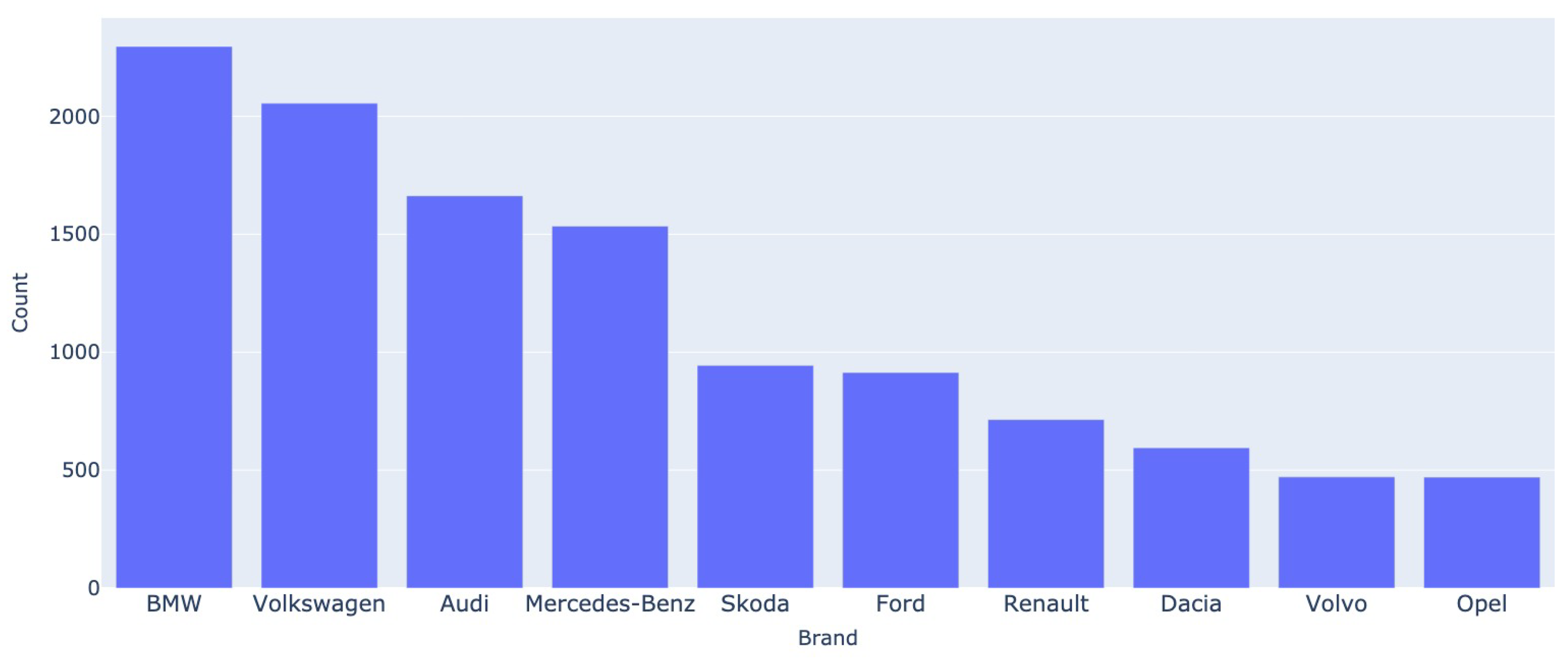
Figure 2.
Most popular 10 brands - Mobile.de
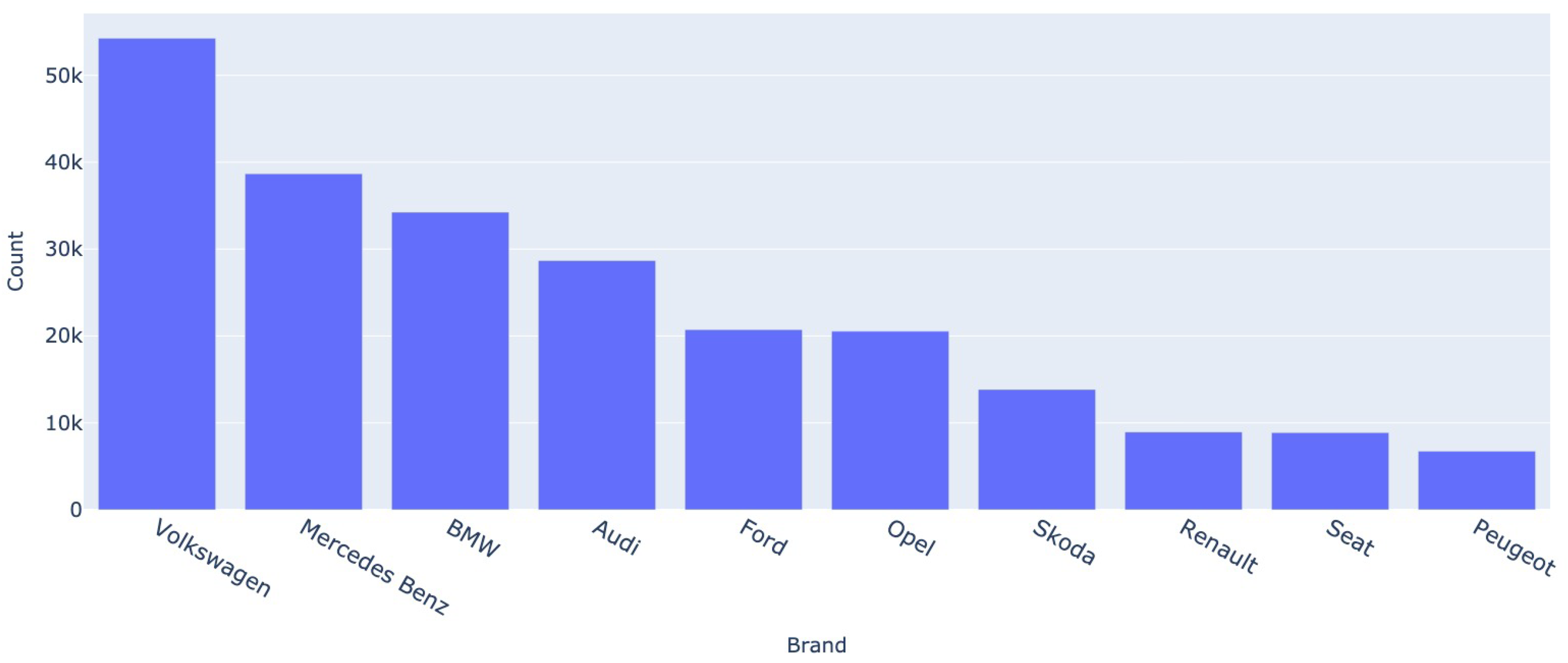
Figure 3.
Year of manufacture - Autovit.ro
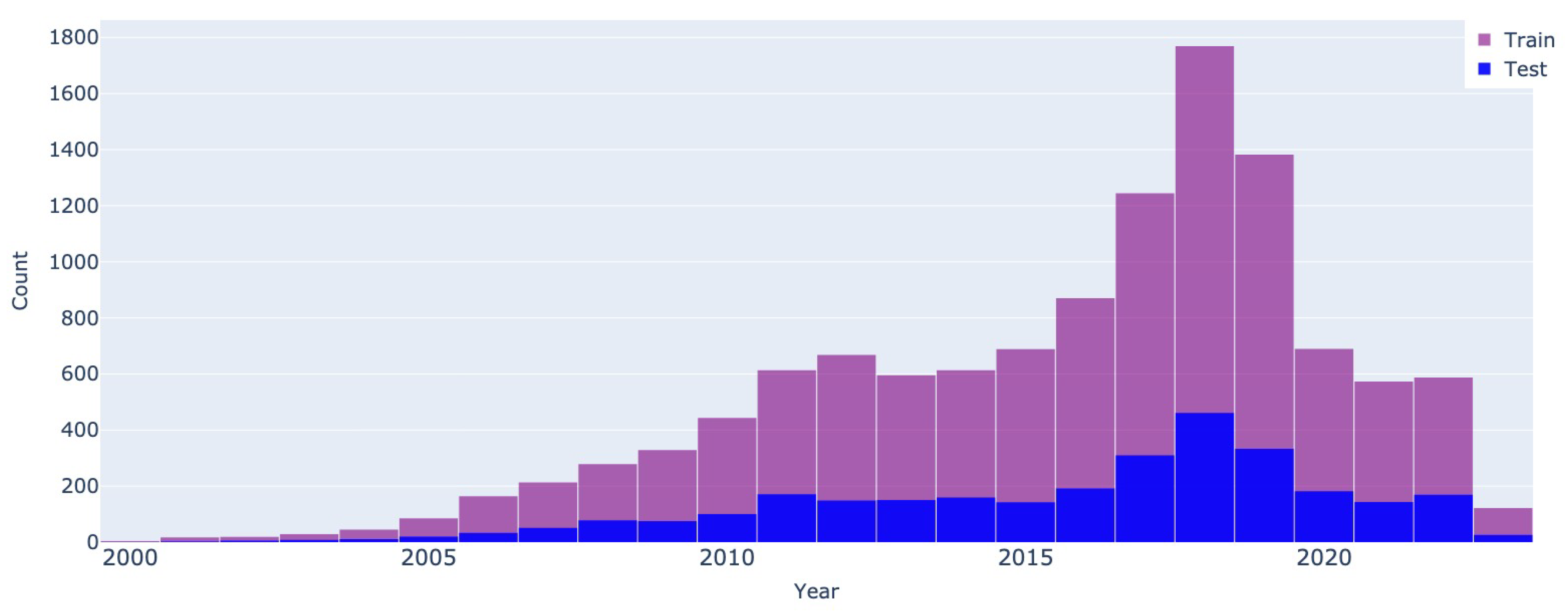
Figure 4.
Year of manufacture - Mobile.de
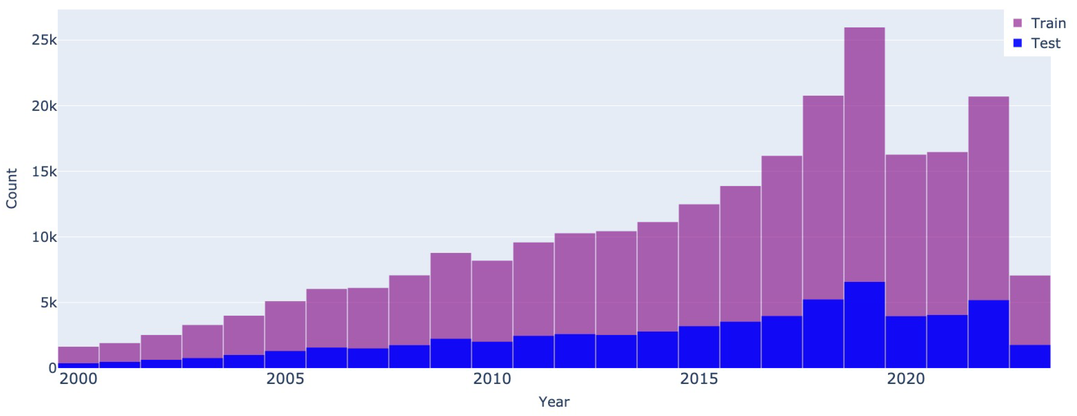
Figure 5.
Mileage - Autovit.ro
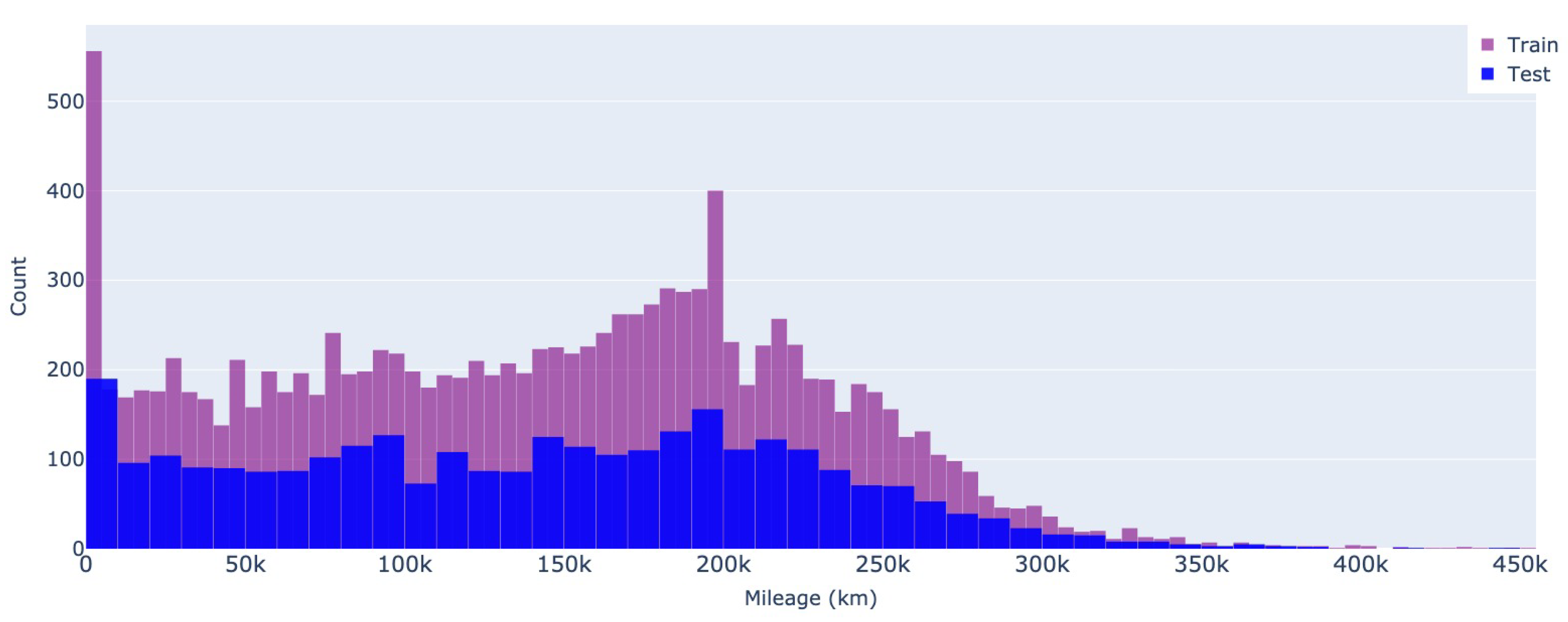
Figure 6.
Mileage - Mobile.de
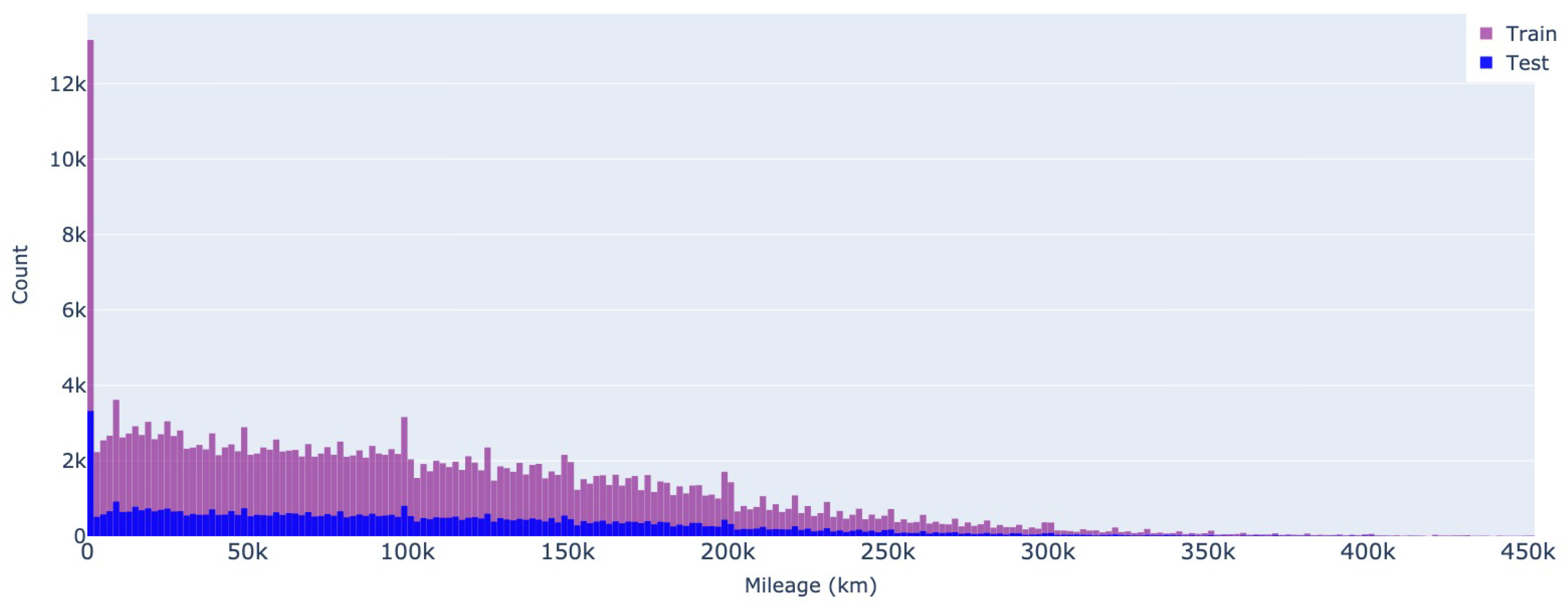
Figure 7.
Engine power - Autovit.ro
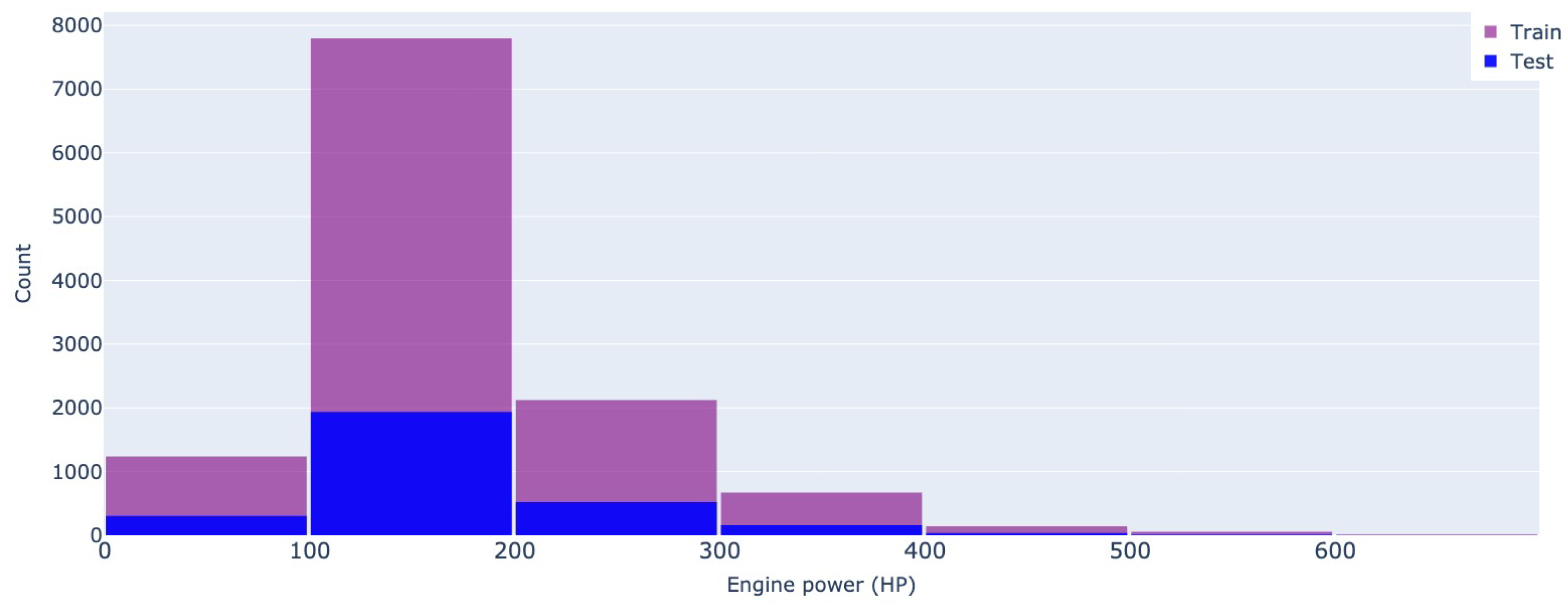
Figure 8.
Engine power - Mobile.de
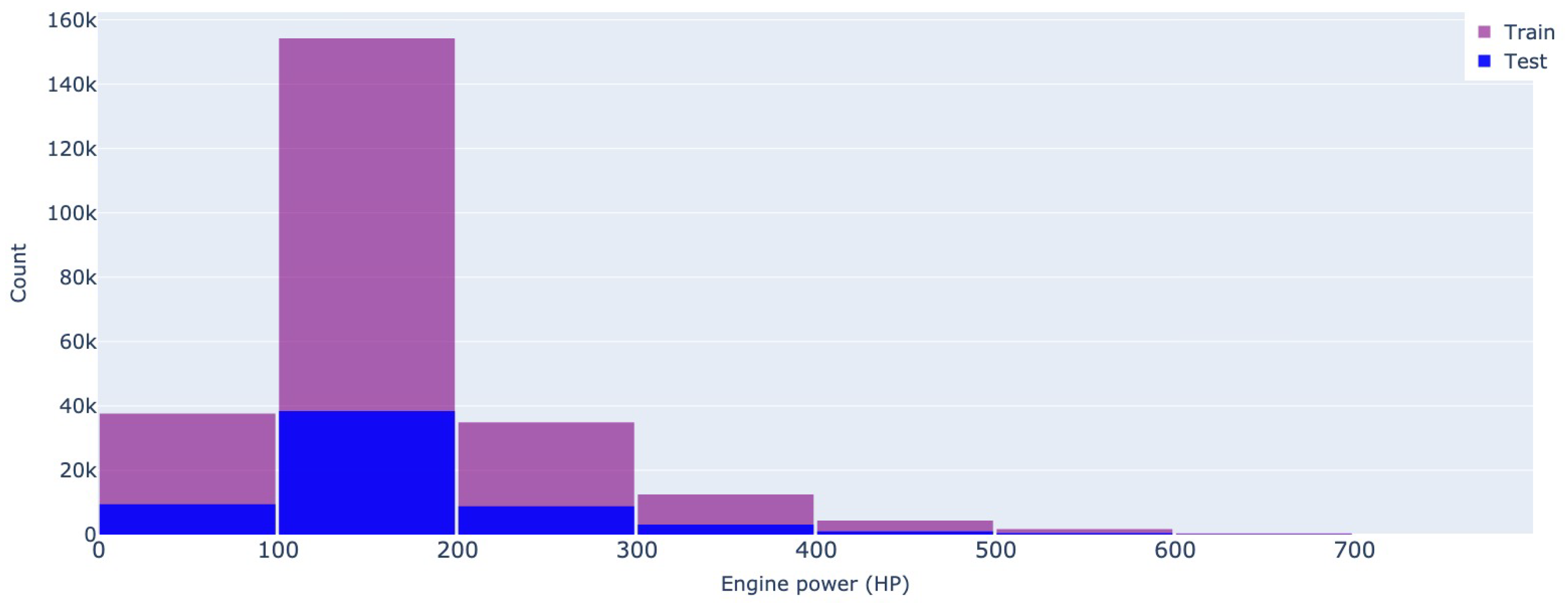
Figure 9.
Car shape - Autovit.ro
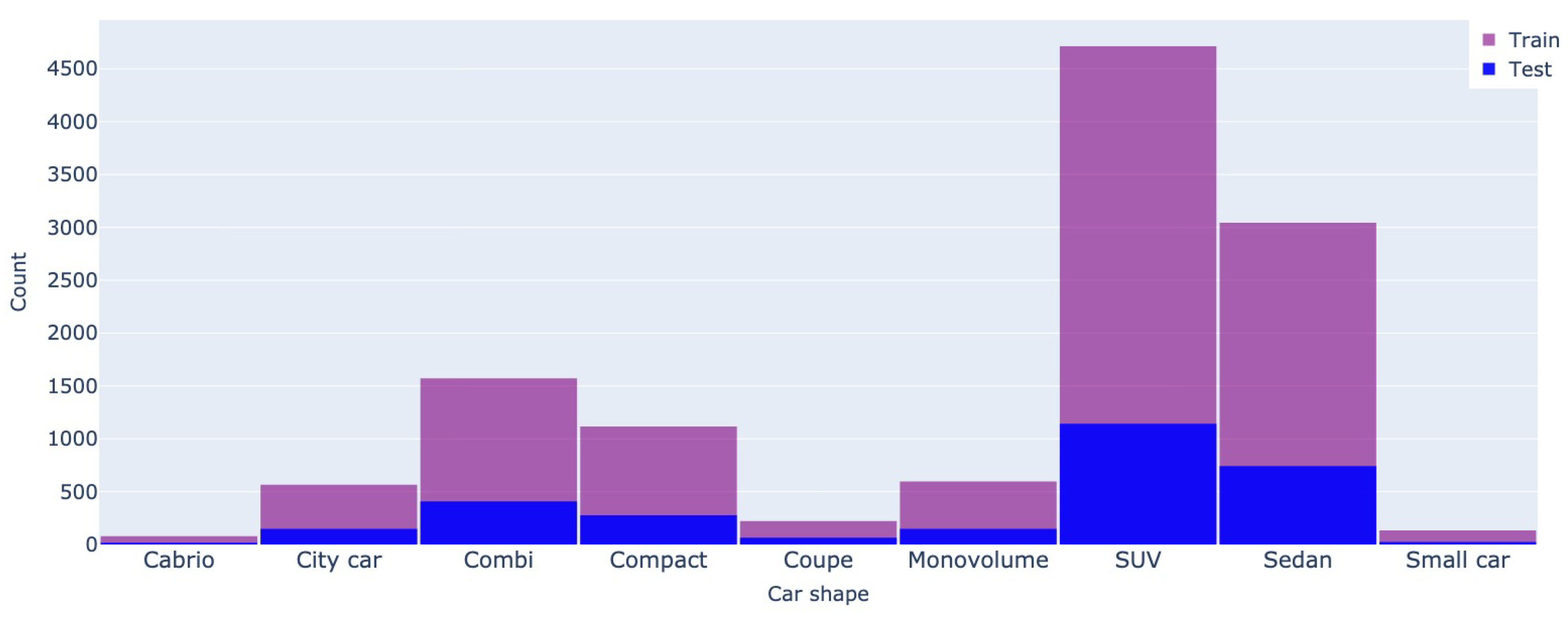
Figure 10.
Car shape - Mobile.de
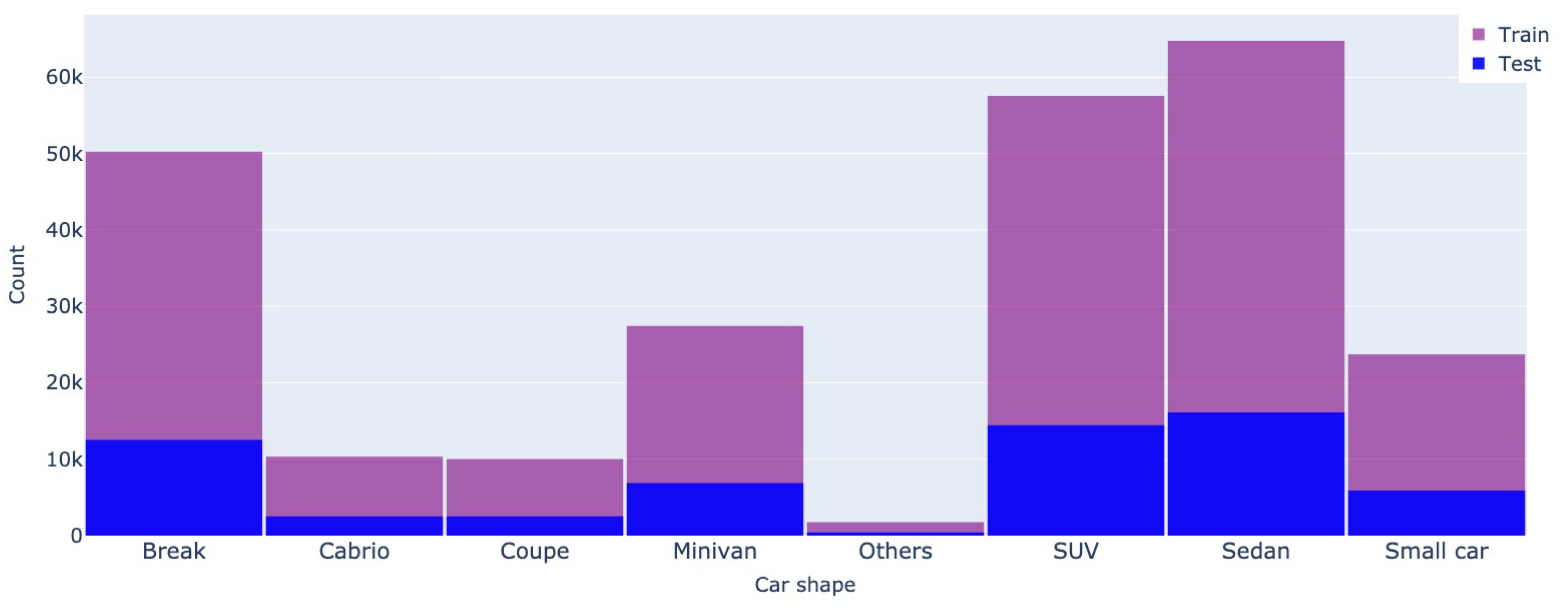
Figure 11.
Color - Autovit.ro
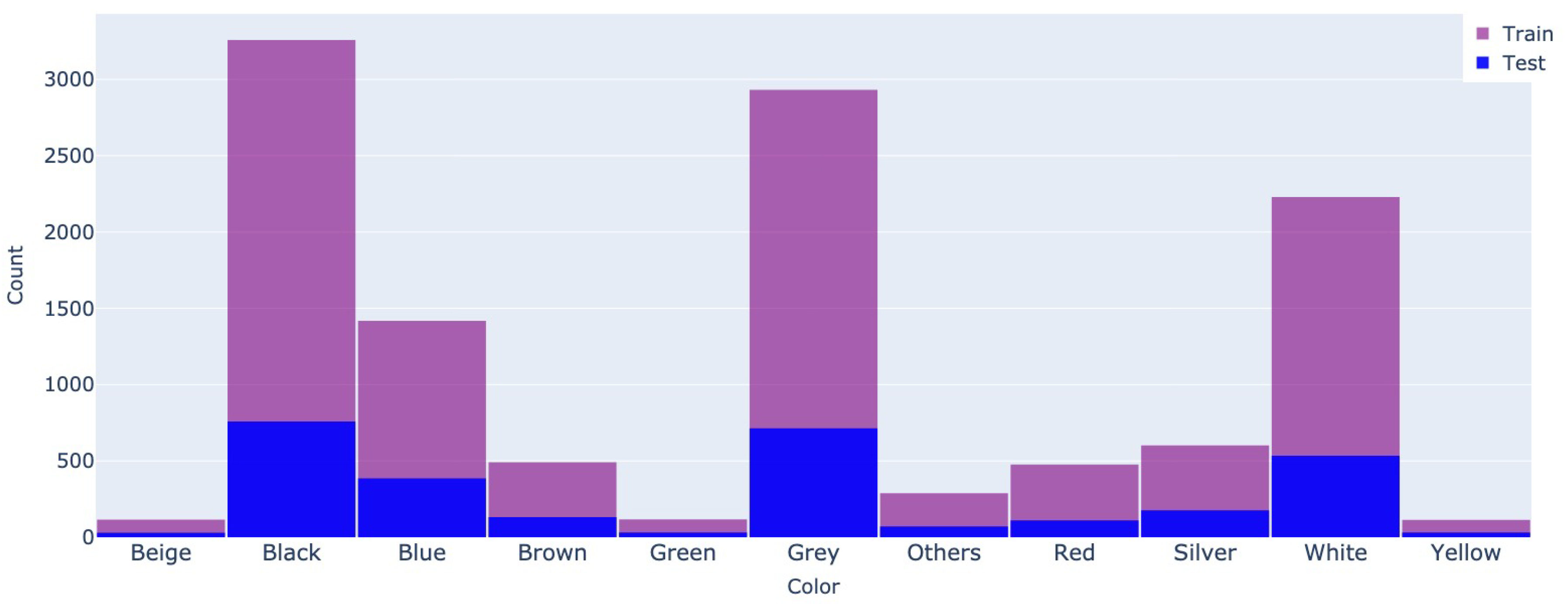
Figure 12.
Color - Mobile.de

Figure 13.
Price distribution - Autovit.ro
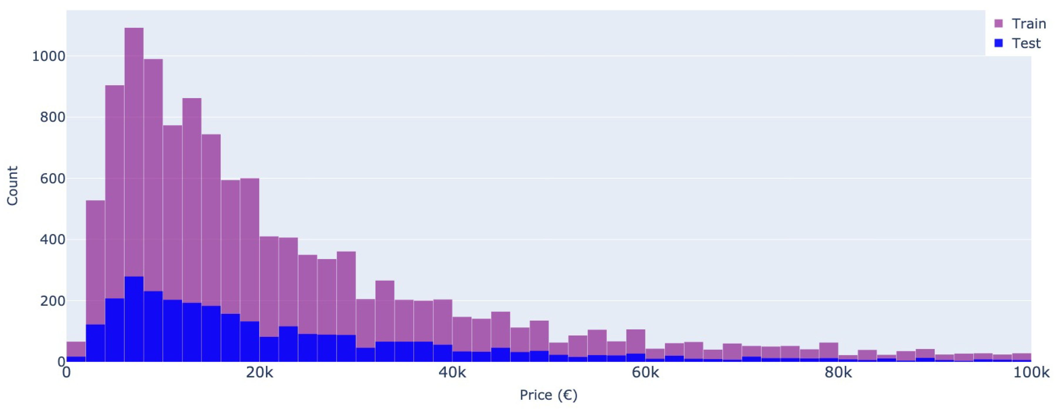
Figure 14.
Price distribution - Mobile.de
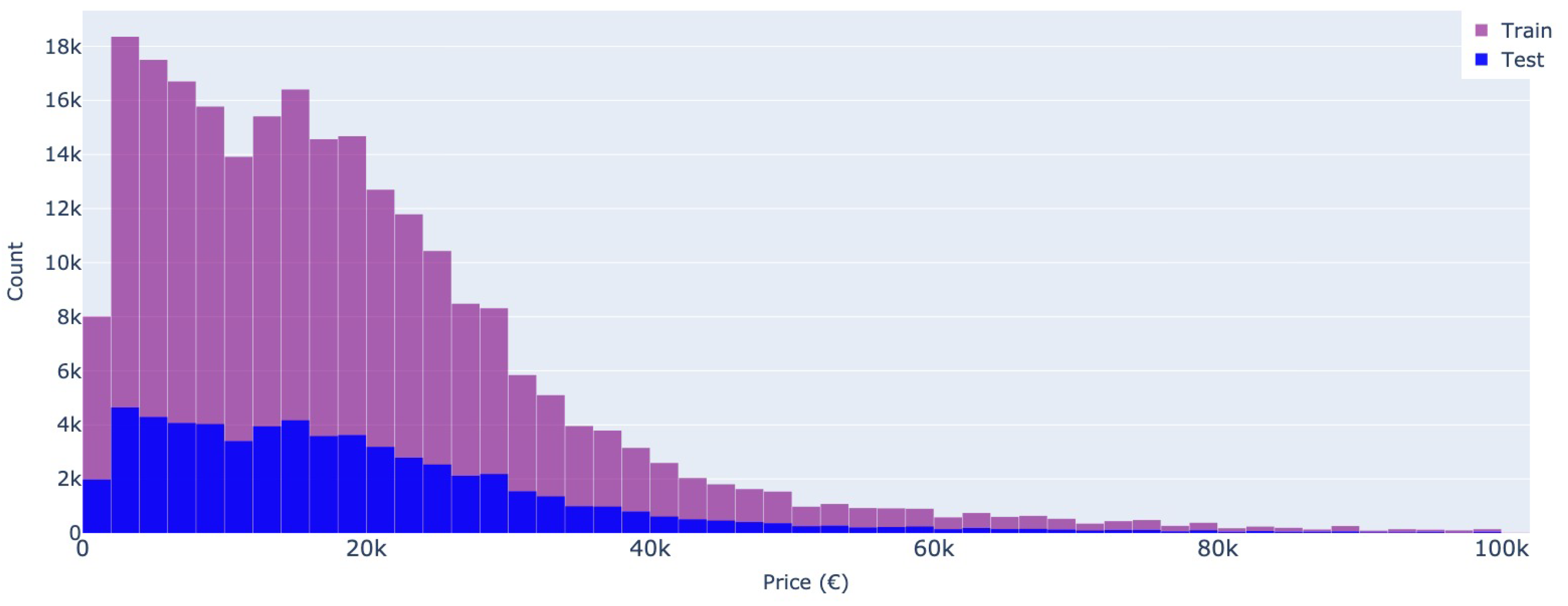
Figure 15.
Price distribution - Most popular brands
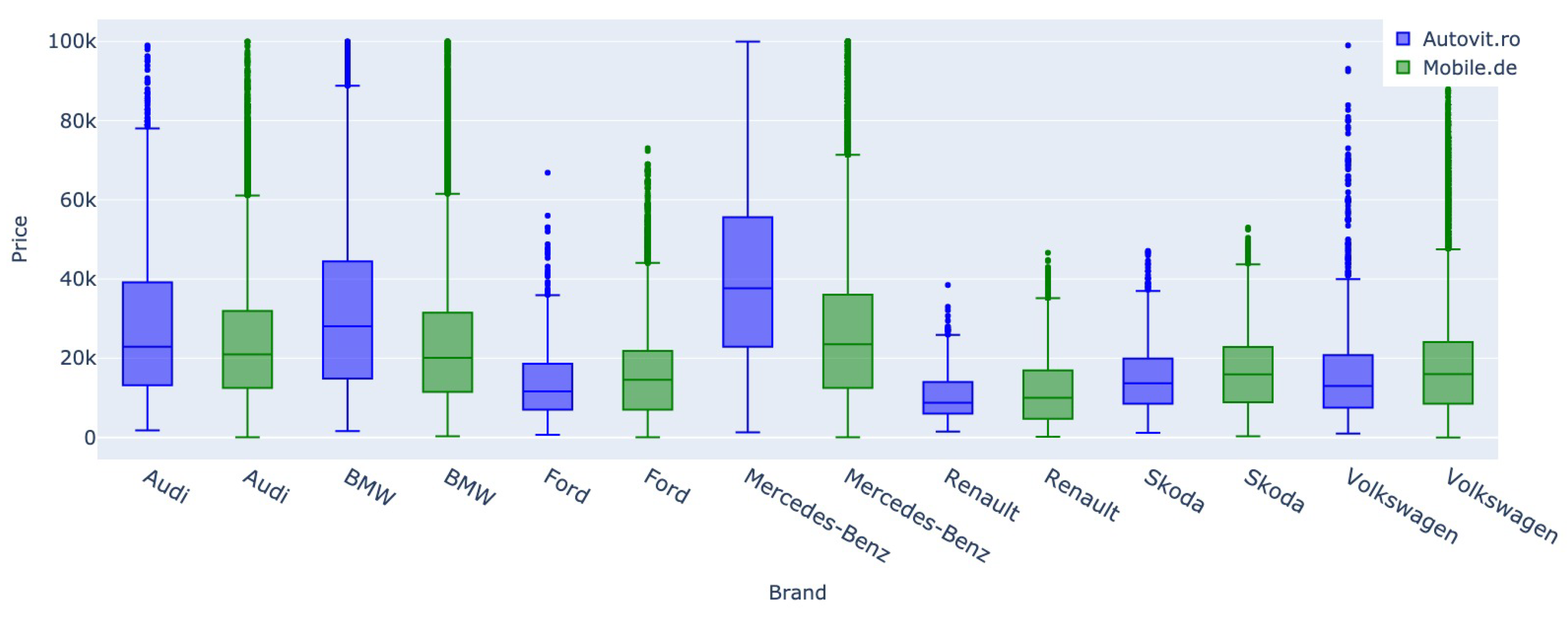
Figure 16.
General architecture overview
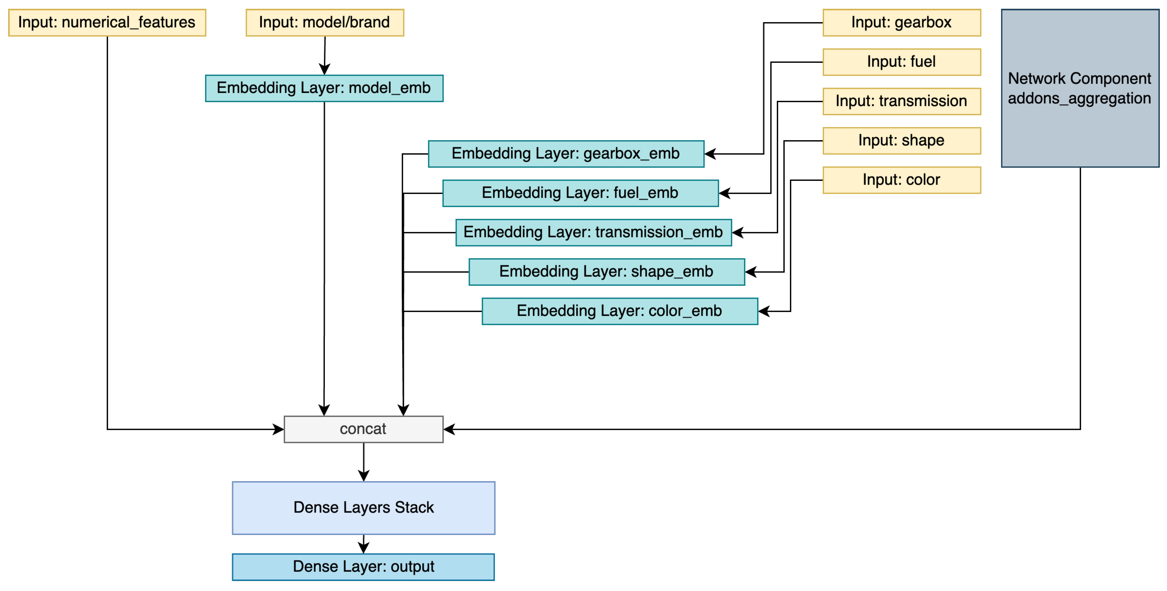
Figure 17.
Hot-encoded add-ons projection component
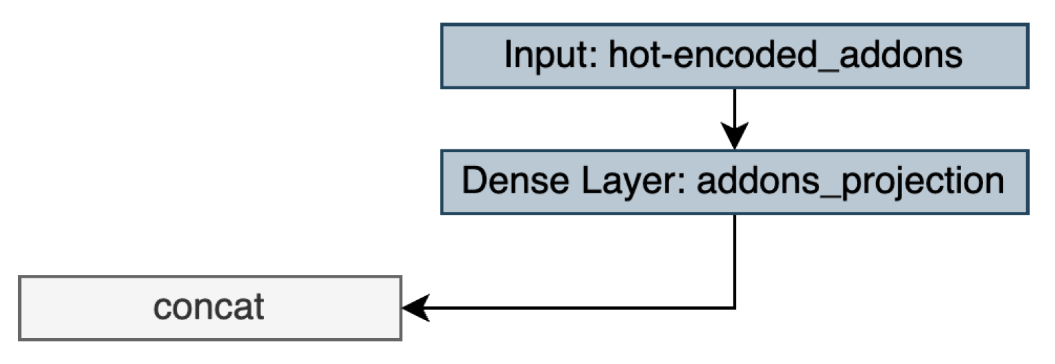
Figure 18.
Mean add-ons embedding component
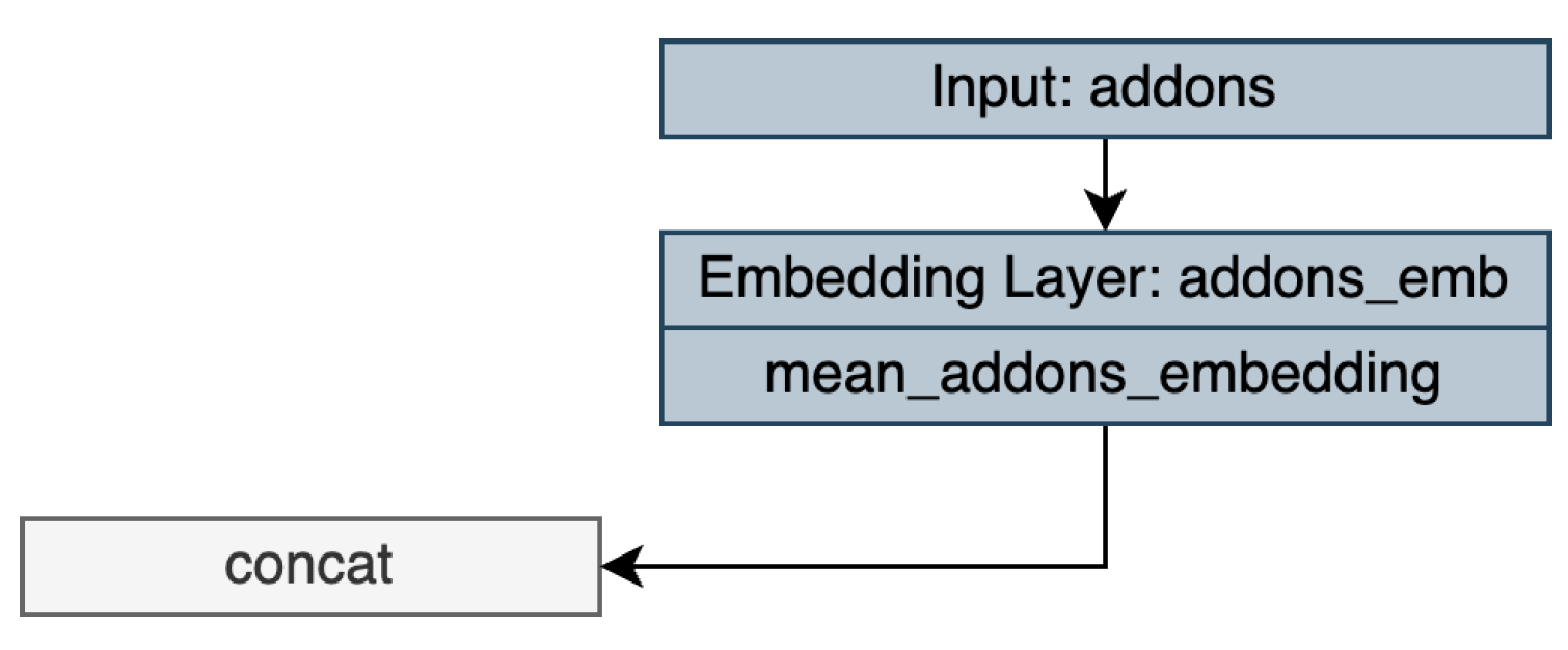
Figure 19.
Add-ons embedding with self-attention component

Figure 20.
Deep neural networks for image and feature analysis architecture
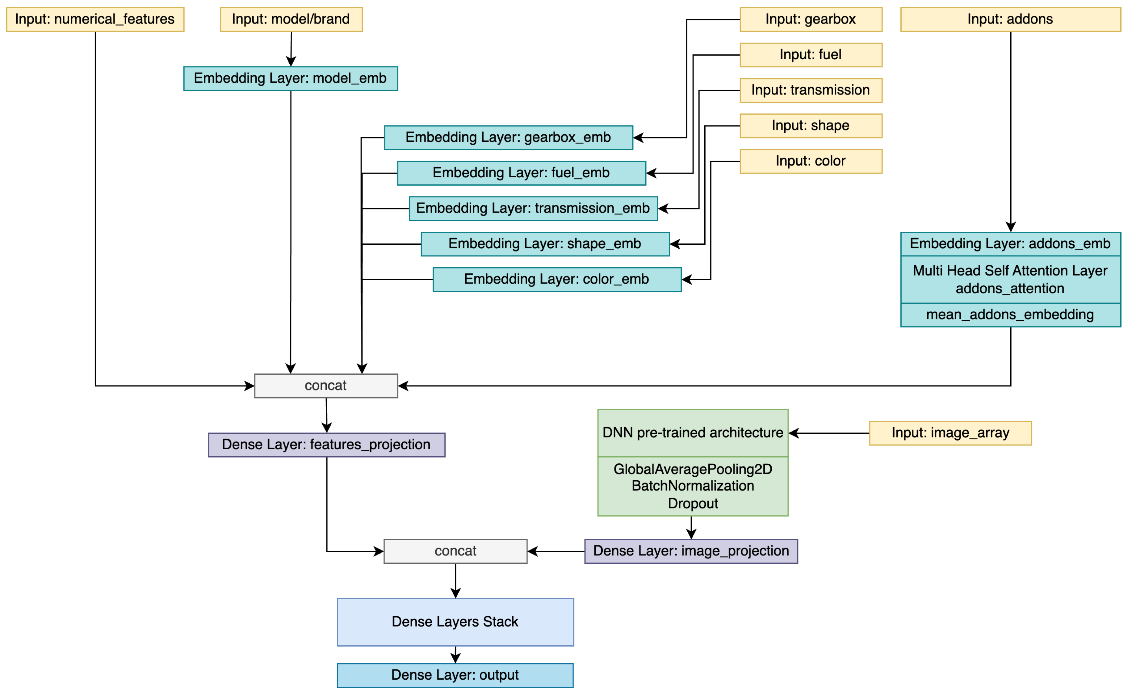
Figure 21.
Deep neural network for image analysis architecture
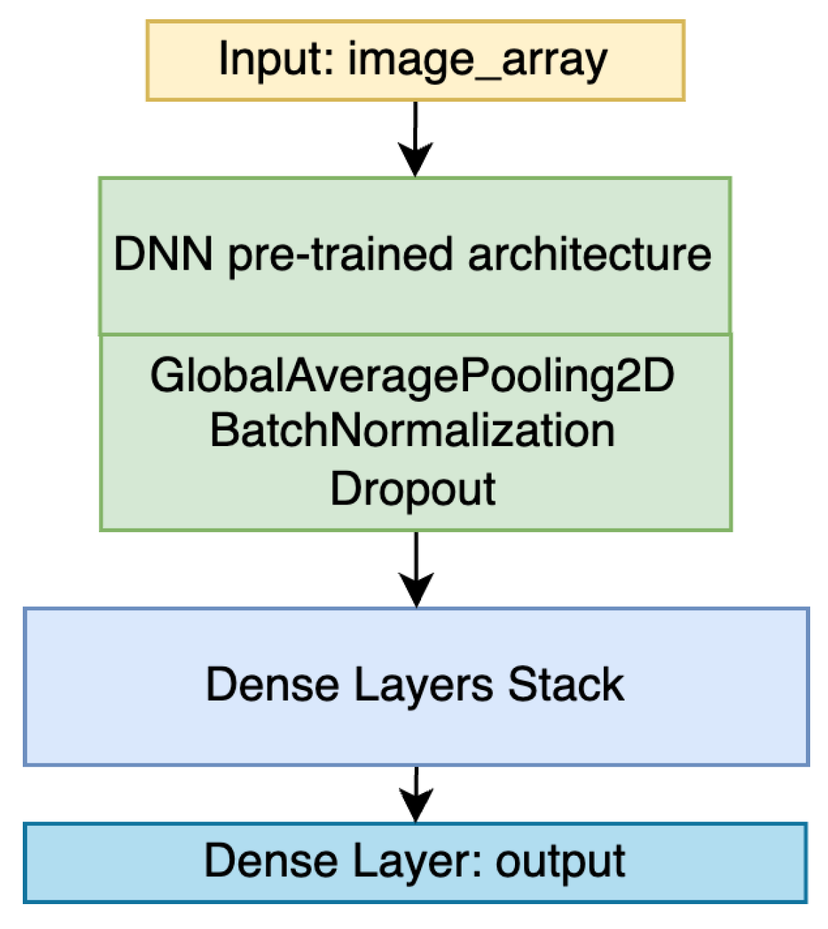
Figure 22.
Q-Q plot - Autovit.ro

Figure 23.
Q-Q plot - Mobile.de
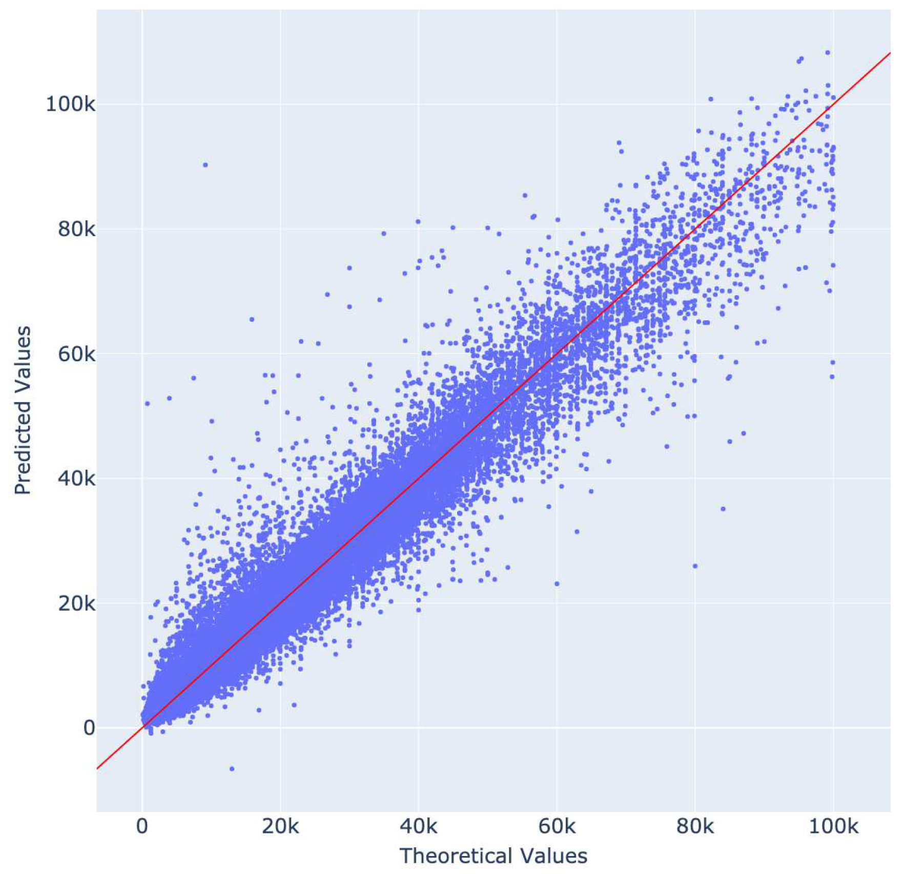
Figure 24.
Mean absolute error by brand - Autovit.ro
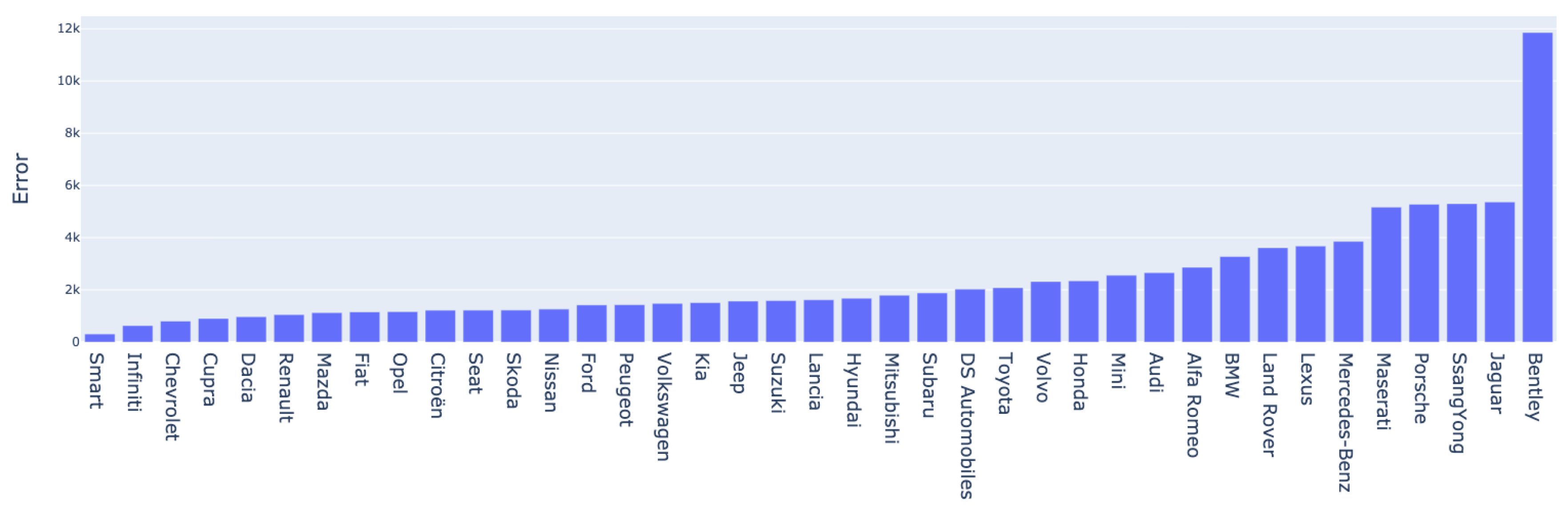
Figure 25.
Mean absolute error by brand - Mobile.de
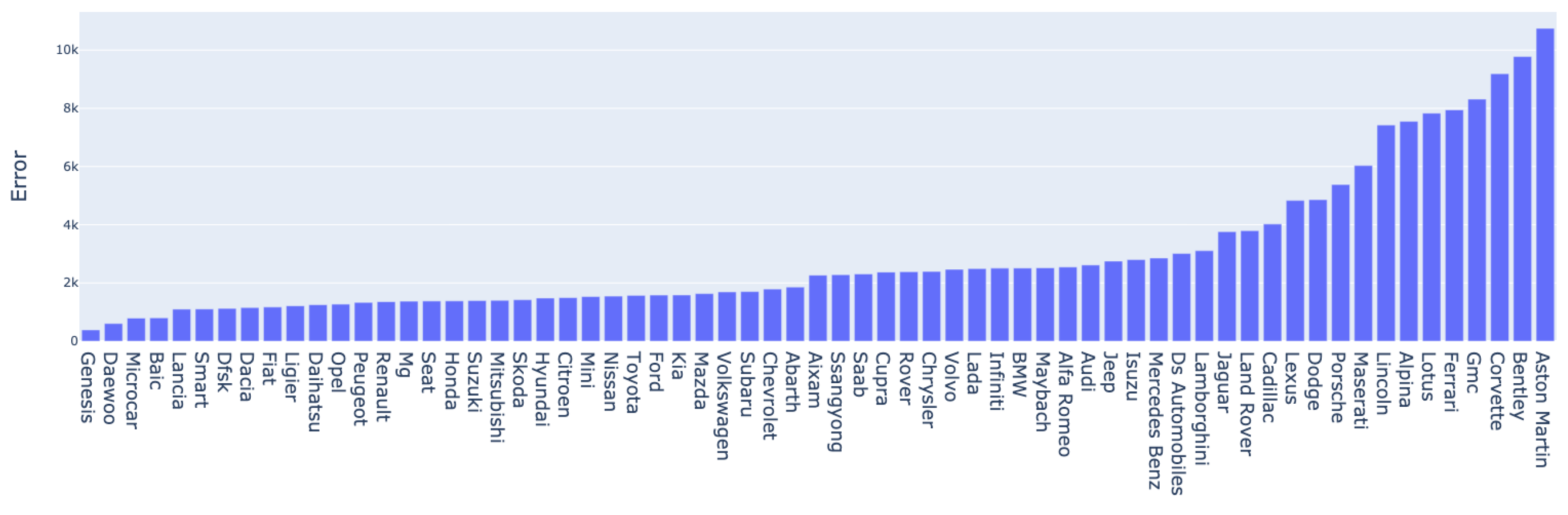

Table 1.
Distribution of specific features.
| Feature | Value | Autovit.ro | Mobile.de | ||||
|---|---|---|---|---|---|---|---|
| Train | Validation | Total | Train | Validation | Total | ||
| Transmission | 2x4 | 6,914 | 1,690 | 8,604 | 192,305 | 47,932 | 24,0237 |
| 4x4 | 5,125 | 1,282 | 6,407 | 53,561 | 13,453 | 67,014 | |
| Fuel | Diesel | 8,445 | 2,082 | 10,527 | 105,842 | 26,442 | 132,284 |
| Gasoline | 2,893 | 683 | 3,576 | 128,643 | 32,172 | 160,815 | |
| Hybrid | 645 | 193 | 838 | 9,545 | 2,310 | 11,855 | |
| LPG | 56 | 14 | 70 | 1,596 | 401 | 1,997 | |
| Others* | 240 | 60 | 300 | ||||
| Gearbox | Automatic | 7,469 | 1,876 | 9,345 | 127,071 | 31,828 | 158,899 |
| Manual | 4,570 | 1,096 | 5,666 | 11,8795 | 29,557 | 148,352 | |
| Engine capacity | <1000 | 508 | 106 | 614 | 22,257 | 5,543 | 27,800 |
| 1000-2000 | 8,743 | 2,183 | 10,926 | 175,479 | 43,902 | 219,381 | |
| 2000-3000 | 2,623 | 642 | 3,265 | 39,488 | 9,780 | 49,268 | |
| 3000+ | 165 | 41 | 206 | 8,642 | 2,160 | 10,802 | |
Table 2.
Most frequent add-ons
| Autovit.ro | Mobile.de | ||
|---|---|---|---|
| Add-on | Count | Add-on | Count |
| ABS | 13,626 | ABS | 300,662 |
| ESP | 13,494 | Power steering | 296,909 |
| Electric windows | 13,428 | Central locking | 295,256 |
| Radio | 12,933 | Electric windows | 293,416 |
| Driver airbag | 12,555 | Electric side mirror | 284,564 |
| Passenger airbag | 12,531 | ESP | 283,250 |
| Side airbag | 12,082 | Isofix | 263,770 |
| Heated exterior mirrors | 12,037 | On-board computer | 258,794 |
| Leather steering wheel | 11,986 | Alloy wheels | 248,468 |
| Isofix | 11,643 | Electric immobilizer | 247,690 |
Table 3.
Feature representation
| Feature | Representation |
|---|---|
| Brand, Model, Gearbox, fuel, transmission, shape, color | Categorical features, represented with an integer as ID |
| Year of manufacture, mileage, engine power, engine capacity | Numerical features, scaled with Z-score in (0, 1) interval |
| Addons | List of categorical features, handled differently based on the approach |
| Images | .jpg file, converted into a 3D array |
| Price | Numerical feature, scaled differently based on the approach |
Table 4.
Results (bold denotes the best model in terms of R2 and MAE).
| Method | Autovit.ro | Mobile.de | ||||
|---|---|---|---|---|---|---|
| R2 | MAE | MedE | R2 | MAE | MedE | |
| XGBoost | 0.92 | 2,965 | 1,613 | 0.91 | 3,102 | 1,772 |
| NN with add-ons projection | 0.95 | 2,463 | 1,391 | 0.94 | 2,050 | 1,236 |
| NN with add-ons embedding | 0.96 | 2,234 | 1,298 | 0.95 | 2,018 | 1,220 |
| NN with self attention on add-ons embedding | 0.96 | 2230 | 1296 | 0.95 | 2,012 | 1,214 |
| EfficientNet for image analysis and self attention on add-ons embedding | 0.96 | 2,369 | 1,350 | 0.95 | 2,030 | 1,231 |
| Swin Transformer for image analysis and self-attention on add-ons embedding | 0.96 | 2,462 | 1,533 | 0.95 | 2,116 | 1,233 |
Table 5.
Validation results after removing one feature (bold denotes features with the highest impact)
Table 5.
Validation results after removing one feature (bold denotes features with the highest impact)
| Model structure | Autovit.ro | Mobile.de | ||||
|---|---|---|---|---|---|---|
| Best architecture without: | R2 | MAE | MedE | R2 | MAE | MedE |
| - | 0.96 | 2,230 | 1,296 | 0.95 | 2,012 | 1,214 |
| Year of manufacture | 0.94 | 3,028 | 1,949 | 0.94 | 2,223 | 1,374 |
| Mileage | 0.95 | 2,723 | 1,600 | 0.93 | 2,481 | 1,589 |
| Engine power | 0.96 | 2,342 | 1,354 | 0.94 | 2,077 | 1,249 |
| Engine capacity | 0.96 | 2,251 | 1,342 | 0.95 | 2,004 | 1,203 |
| Addons | 0.96 | 2,401 | 1,401 | 0.93 | 2,264 | 1,370 |
| Fuel | 0.96 | 2,278 | 1,336 | 0.95 | 2,007 | 1,200 |
| Transmission | 0.96 | 2,243 | 1,337 | 0.95 | 2,018 | 1,221 |
| Gearbox | 0.96 | 2,270 | 1,331 | 0.94 | 2,046 | 1,248 |
| Car shape | 0.96 | 2,271 | 1,315 | 0.94 | 2,051 | 1,218 |
| Color | 0.96 | 2,299 | 1,334 | 0.95 | 2,011 | 1,202 |
Table 6.
Validation results after adding one feature (bold denotes features with the highest impact)
Table 6.
Validation results after adding one feature (bold denotes features with the highest impact)
| Model structure | Autovit.ro | Mobile.de | ||||
|---|---|---|---|---|---|---|
| Brand/Model with: | R2 | MAE | MedE | R2 | MAE | MedE |
| - | 0.57 | 8,761 | 5,697 | 0.57 | 7,015 | 5,182 |
| Year of manufacture | 0.92 | 3,444 | 1,930 | 0.87 | 3,450 | 2,240 |
| Mileage | 0.88 | 4,419 | 2,872 | 0.84 | 3,955 | 2,637 |
| Engine power | 0.72 | 6,525 | 3,559 | 0.75 | 4,958 | 3,226 |
| Engine capacity | 0.63 | 7,930 | 4,947 | 0.67 | 5,828 | 3,880 |
| Addons | 0.82 | 5,181 | 2,927 | 0.87 | 3,374 | 2,124 |
| Fuel | 0.62 | 8,010 | 5,052 | 0.61 | 6,651 | 4,852 |
| Transmission | 0.60 | 8,395 | 5,215 | 0.58 | 7,083 | 5,338 |
| Gearbox | 0.61 | 8,113 | 4,725 | 0.63 | 6,427 | 4,583 |
| Car shape | 0.59 | 8,546 | 5,476 | 0.60 | 6,804 | 4,945 |
| Color | 0.59 | 8,659 | 5,669 | 0.59 | 6,784 | 4,873 |
| Images (EfficientNet architecture) | 0.69 | 6,899 | 4,053 | 0.82 | 4,045 | 2,658 |
| Images (Transformers architecture | 0.67 | 7,534 | 4,335 | 0.82 | 4,087 | 2,697 |
Table 7.
Validation results for transfer learning
| Method | Autovit.ro | ||
|---|---|---|---|
| R2 | MAE | MedE | |
| DNN for image analysis without pre-training | 0.69 | 6,899 | 4,053 |
| DNN for image analysis with pre-training and fine-tuning | 0.79 | 5,652 | 3,373 |
Disclaimer/Publisher’s Note: The statements, opinions and data contained in all publications are solely those of the individual author(s) and contributor(s) and not of MDPI and/or the editor(s). MDPI and/or the editor(s) disclaim responsibility for any injury to people or property resulting from any ideas, methods, instructions or products referred to in the content. |
© 2023 by the authors. Licensee MDPI, Basel, Switzerland. This article is an open access article distributed under the terms and conditions of the Creative Commons Attribution (CC BY) license (http://creativecommons.org/licenses/by/4.0/).
Copyright: This open access article is published under a Creative Commons CC BY 4.0 license, which permit the free download, distribution, and reuse, provided that the author and preprint are cited in any reuse.


