
Submitted:
04 June 2023
Posted:
05 June 2023
You are already at the latest version
Abstract
This manuscript presents a system that can generate a 2D grid map and a 3D voxel model of an environment by fusing multiple sensors integrated into a robot. The fusion of these sensors is done by utilizing Robot Operating System (ROS) and some of its libraries. The sensors that are fused in the robot are a Light Detection and Ranging (LIDAR), Inertial Measurement Units (IMU), wheel encoders, and a Time-of-Flight camera. With the fusion of the point cloud data information obtained with the Time-of-Flight camera, the laser information of the LIDAR sensor, in addition to the odometry generated with the other sensors, a 2D grid map and a 3D model of two different environments were created, thus testing the performance of the system.
Keywords:
time-of-flight
; LiDAR
; indoor mapping
; ROS
; SLAM
1. Introduction
Mobile robot technology has advanced significantly and brought in a lot of study in recent years. Mobile robots have the ability to navigate and explore new environments by simultaneously constructing a map and tracking their own position. This capability is made possible through Simultaneous Localization and Mapping (SLAM) [1], which enables the robot to estimate its location in the environment by utilizing on-board sensors like LIDAR, IMU, and wheel encoders. By integrating sensor data, SLAM allows the robot to create an accurate map of the surroundings while simultaneously determining its own position within that map.
SLAM is the task of constructing a map of an unknown environment and localizing the sensor in the map. There have been multiple studies that include vision-based methods and LIDAR-based methods. These methods can employ one or multiple sensors to accurately generate a map of the environment, but single-sensor systems have limitations. When a camera is employed, it depends on its capability to visualize the environment. On the other hand, the information provided by LIDAR sensors can have problems positioning in unstructured environments. Finally, the movement and long-term error accumulation invalidates the odometer. To solve this problem is required the implementation of additional sensors such as IMU, GPS, and UWB. Most mobile robots employ IMU, which includes an accelerometer, magnetometer, and gyroscope, and is capable of measuring acceleration, orientation, and angular velocity allowing it to be a low-cost implementation.
2D LIDAR SLAM systems can be implemented with different packages like GMapping [2], which employs a Rao-Blackwellized particle filter to generate 2D grid maps from LIDAR information. Hector SLAM [3], a popular ROS-based SLAM, and Cartographer [4] are the most popular systems. In our project, the package employed to generate a 2D grip map of the environment was Hector SLAM.
Hector SLAM is an open-source algorithm utilized for creating a 2D grid map of the surrounding environment using LIDAR. This algorithm relies on scan matching instead of wheel odometry to determine the robot’s position. The high update rate of the LIDAR enables fast and precise robot localization through scan matching.
The Vision SLAM (vSLAM) variant [5] focuses on the use of a camera as a sensor to extract data from the environment. Monocular, stereo, and RGB-d cameras are the most used cameras in this variant. Moreover, some studies employ Time-of-Flight (ToF) [6] cameras instead of the previously mentioned ones. In addition, the vSLAM models can be complemented with a 3D accelerometer to become a visual and inertial SLAM.
Time-of-Flight (TOF) is a 3D imaging technique that operates on a similar principle to 3D laser sensors. It offers a significant advantage in that it can capture depth information for the entire scene simultaneously, rather than relying on point-wise scanning. This makes TOF cameras well-suited for dynamic scenes. The output of a TOF camera is a depth image where the distance between a point and the corresponding point in the scene is represented by each pixel [7]. This technology has found application in various fields of research and investigation. Some of its practical applications may include robot navigation [8], recognition of barriers in no-structured environments with no previous training [9], and SLAM [10].
A 2D map representation could not be enough to display all the information of a zone since it is not able to properly generate visualizations of some structures, such as stairs and windows. On the other hand, a 3D model can generate these structures that the 2D model is not able to do, providing the observer with a more accurate view of the captured scene. 3D models are well-suited for various tasks, including surveillance, security, rescue applications, and self-localization, due to their versatility and applicability in these domains.
There have been some implementations that fuse ToF cameras with RGB or stereo cameras to generate proper depth images. Zhao et al. [11] proposed a model combining a binocular camera, novel ToF camera, and emerging 16-line LiDAR to generate a dense depth image. In their work, Benet et al. [12] combined an RGB camera, a LiDAR sensor, and a TOF camera to perform both colorimetric and geometric measurements on detected objects. This approach allowed them to identify various objects, including grass, leaves, and tree branches, located in front of a vehicle. Also, Jung et al. [13] employed a ToF camera combined with a stereo camera. In this case, the 3D map is generated from only one image, so it is not suited for environment generation. In our model, we also use the robot’s odometry to combine image sequences and generate the environment in real-time.
In this manuscript, we proposed a model which can generate a 2D and 3D map simultaneously with the use of a Time-of-Flight camera, a 2D LIDAR sensor, a 6-DOF accelerometer and gyroscope IMU, and the information of wheel encoders of a robot. This model was run on two Raspberry Pi 4 model B since one is not enough to handle all the information provided by the sensors.
The organization of this manuscript is article is the following: the related work about indoor mapping is summarized in Section 2. In Section 3 is introduced different SLAM algorithms and implementations that have been made over time. Section 4 describes the time-of-flight algorithm. Section 5 describes the hardware and software employed. Section 6 introduces the methodology to start the map generation. Next, in Section 7, an analysis of the system working is performed. Lastly, in Section 8, the conclusion and future work is described.
2. Related Work
In the last few years, there have been many SLAM works using LIDAR-based multi-sensor fusion to achieve a more precise and stable system. Xu et al. [14] presented in detail the basic principles and recent works on 3D LiDAR-based multisensor fusion SLAM. Also, some SLAM datasets were reviewed, and five open-source algorithms and their performances were compared using the UrbanNav dataset.
There are multiple 2D and 3D LIDAR-based methods. LOAM [15] is an optimized approach specifically designed for real-time odometry and mapping using LIDAR data only. The proposed method has been validated through experiments conducted on the KITTI odometry benchmark and a campus environment. The experiments shown that the T-LOAM (Time-of-Flight LIDAR Odometry and Mapping) algorithm offers real-time performance and outperforms existing LiDAR odometry frameworks in terms of segmentation and mapping precision.
Macario Barros et al. [16] conducted an examination of the three primary visual-based algorithms, namely visual-inertial, visual-only, and RGB-D SLAM. The fundamental algorithms of each approach were also evaluated utilizing flowcharts and diagrams, emphasizing the key benefits associated with each technique. In addition, the following six criteria were provided to influence accuracy, system sizing and hardware design: map density, algorithm type, global optimization, availability, loop closure, and embedded implementations. These criteria facilitate the analysis of the SLAM algorithm and consider both the hardware and software level.
ORB-SLAM3 [17] was the pioneering system capable of performing visual, visual-inertial, and multimap SLAM using stereo, monocular, and RGB-D cameras, utilizing both pin-hole and fisheye lens models. The system introduced two significant advancements. Firstly, it featured a tightly integrated visual-inertial SLAM system that relied entirely on maximum a posteriori estimation, ensuring robust real-time operation in various environments, both indoors and outdoors, and offering two to ten times greater accuracy compared to previous approaches. Secondly, it incorporated a multi-mapping system based on a novel memory-enhanced location recognition method, enabling ORB-SLAM3 to persist even during extended periods of sparse visual information. In cases of lost tracking, ORB-SLAM3 initiates a new map that seamlessly merges with previous maps upon revisiting.
Visual-based SLAM frameworks, like the one presented in reference [18] utilize monocular, stereo, or RGB-D cameras to create real-time maps of the surrounding environment. These frameworks are capable of mapping diverse environments, ranging from indoor settings with limited manual movements to industrial environments with flying drones or city landscapes with moving vehicles. Additionally, these methods demonstrate strengths in loop-closure detection. Nonetheless, their reliability for autonomous tasks without supplementary sensors is compromised due to sensitivity towards illumination variations and limited range capabilities.
Another well-known RGB-D SLAM system that gained significant recognition was KinectFusion [19]. This approach involved the fusion of depth data from a Kinect sensor into a unified global implicit surface model of the observed environment in real-time. The resulting model was utilized to track the camera’s pose using Iterative Closest Point (ICP) algorithms. However, KinectFusion had certain limitations. It was primarily suitable for small workspaces due to its volumetric representation, which imposed constraints on scalability. Additionally, the absence of loop closing mechanisms posed challenges in handling larger and more complex environments.
Gupta and Li [20] conducted a study with the objective of developing an indoor mapping system for data collection in indoor environments. Their focus was on exploring new scanning devices that are both efficient and cost-effective. The study involved testing the performance of a Kinect sensor and a StereoLab ZED camera, comparing them across various factors such as accuracy, resolution, speed, memory usage, and their ability to adapt to different lighting conditions. Their advantages and disadvantages compared to conventional scanning devices were also analyzed.
As some 3D LIDAR-based methods are mentioned, Tee and Han [21] conducted a comprehensive review and comparison of prevalent 2D SLAM systems in an indoor static environment. Their evaluation employed ROS-based SLAM libraries on an experimental mobile robot equipped with a 2D LIDAR module, IMU, and wheel encoders. The study focused on analyzing three algorithms: Hector-SLAM, Google Cartographer, and Gmapping. The article delves into the strengths and weaknesses of these algorithms while visually illustrating the disparities in terms of the generated maps.
3. Simultaneous localization and mapping
SLAM has garnered significant attention as a prominent research area in the past few decades. The initial research concept of SLAM emerged with the aim of enabling autonomous control for mobile robots [22]. Subsequently, SLAM applications have been extensively explored in various domains, including augmented reality, computer vision modelling, and self-driving cars [23].
The solutions that have obtained the best results when dealing with the SLAM problem are those based on probabilistic techniques. This type of algorithm is based on Bayes’ theorem, which relates the marginal and conditional probabilities of two random variables.
The Kalman filter is designed under the assumption that the noise affecting the data follows a Gaussian distribution. It is primarily employed to address linear system problems and finds application in SLAM, showcasing notable convergence properties. However, when dealing with nonlinear filtering systems like SLAM, the Extended Kalman filter (EKF) is frequently utilized. In their work, Ullah et al. [24] put forth two primary localization algorithms: Kalman Filter SLAM and EKF SLAM. Through simulations, these algorithms were evaluated and demonstrated to be effective and feasible options for SLAM applications. Furthermore, Montemerlo et al. [25] introduced a novel model known as FastSLAM, which combines a particle filter and the Extended Kalman Filter (EKF) to handle non-linear systems with non-Gaussian characteristics. FastSLAM is an iterative algorithm that enables the estimation of the complete posterior distribution over both the robot’s pose and landmark locations. By utilizing the particle filter approach, FastSLAM offers an effective solution for SLAM problems, accommodating uncertainties and non-linearity in the environment.
Various filters are employed in SLAM techniques to facilitate effective implementation. One such filter is the Rao-Blackwellized Particle Filter (RBPF) [26], which combines the strengths of both particle filters and Kalman filters. RBPF is commonly utilized in SLAM applications to handle the challenge of particle reduction, ensuring efficient estimation and tracking. Additionally, the Kullback-Leibler Distance (KLD) [27] sampling algorithm is employed in SLAM applications for effective particle reduction. This algorithm aids in maintaining a representative set of particles while discarding redundant or less informative particles, thus improving the efficiency and accuracy of SLAM algorithms. Grisetti et al. [28] presented an adaptive technique for reducing the number of particles in an RBPF for learning grid maps. Taking into account the movement of the robot and the most recent observation, an approach to compute accurate proposal distribution is proposed. Together, these methods contribute to the advancement of SLAM techniques, enabling better particle management and enhancing the overall performance of SLAM systems.
Milford et al. [29] presented RatSLAM, an implementation of a hippocampal model that can perform SLAM in real-time. The mentioned model was employed to identify distinctive and ambiguous landmarks, incorporating a competitive attractor network. This network allowed for the seamless integration of odometric information and landmark sensing, ensuring consistent representation of the environment.
Vision SLAM refers to those SLAM systems that use cameras as the main input sensor to receive information about the environment. Mono-SLAM [30] is a top-down Bayesian framework for single-camera localization that uses a motion modeling and an information-guided active measurement strategy for a parsed set of natural features. ORB-SLAM [31] is a modified version of Mono-SLAM that operates on extracted features using the ORB key-point feature descriptor algorithm. It leverages the ORB algorithm for robust feature matching and tracking in single-camera setups. Additionally, ORB-SLAM2 [32] extends its capabilities to provide enhanced assistance for RGB-D camera and stereo configurations. This allows ORB-SLAM2 to leverage depth information from those sensors to obtain an improvement in the robustness and accuracy of the SLAM system.
Direct methods for visual SLAM refer to techniques that eschew the conventional approach of searching for key points in images. Instead, these methods utilize image intensities to estimate the camera’s position and the surrounding environment. Engel et al. [33] introduced a direct monocular SLAM method known as Large-Scale Direct Monocular SLAM (LSD-SLAM). This algorithm relies solely on RGB images captured by the camera to gather information about the environment. It incrementally constructs a graph-based topographic map.
L-SLAM (6-DoF Low Dimensionality SLAM) introduced in [34] is a variant of the FastSLAM family of algorithms with reduced dimensionality. In contrast to FastSLAM algorithms that employ Extended Kalman Filters (EKF), L-SLAM updates its particles using linear Kalman filters. This approach is possible because L-SLAM utilizes odometry information to sample the new robot orientation within the particle filter. The resulting approximation, derived from the linear kinematic model of the vehicle’s 6 degrees of freedom (6DoF), can be effectively estimated implementing a Kalman filter.
4. Time of Flight
The fundamentals of ToF imaging, as illustrated in Figure 1 [35], involves the emission of Infra-Red (IR) light from an LED towards an object in the scene. The surface of the object reflects the light, which is then detected by the ToF sensor. The distance to the object is determined by measuring the phase difference or delay between the emitted and reflected IR lights. Kolb et al. [36] provided formulations for sinusoidal signals to calculate the phase change. This calculation is based on the relationship between the four control signals and the corresponding electric charge values. Each pixel on the sensor samples the amount of light reflected by the scene four times at equal intervals during each period, enabling parallel measurement of its phase.
where are the sensor samples reflected in four periods of time. The distance to the object can be calculated as follows:
where c is the speed of light in a vacuum and f is the frequency of the light signal. constrains the maximum distance of measurement without phase wrapping.
ToF cameras are an alternative to classical depth sensors, which can provide depths image at high frame rates. ToF cameras evaluated the "time-of-flight" of a light signal produced by the camera and reflected from each point in the scene to determine the 3D location of each point. ToF cameras are small and have no mechanical components. As a result, they can be easily miniaturized for use in mobile devices such as smartphones and tablets.
3D LiDAR sensors emit rapid laser signals, sometimes up to 150,000 pulses per second, which bounce back from an obstacle. A sensor measures the amount of time it takes for each pulse to bounce back. Some of its advantages include accuracy and precision. LiDAR is extremely accurate compared to cameras because shadows, bright sunlight, or the oncoming headlights of other cars don’t fool the lasers. And disadvantages include cost, large size, interference, traffic jams, and limitations in seeing through fog, snow, and rain.
High-resolution LiDARs have a greater range than ToF but are more expensive. Lower-resolution solid-state flash LiDARs have a greater range than ToF but have poorer resolution and depth precision.
5. Materials
Different hardware and software were required to create 2D and 3D map visualization. Figure 2 shows the connections required to make the system work.
The following subsections, the sensors, and the boards required will be described.
5.1. Sensors
To get a correct visualization and orientation of the robot, the following sensors are required: LiDar, Time-of-Flight camera, Inertial Measurement Unit, and Wheel encoder.
5.1.1. LiDAR
LiDAR is a laser scanner that measures the distance between the point of emission of that laser and an object or surface. The distance is determined by measuring the time delay between the emission of the pulse and its detection through the reflected signal. One of the advantages of LiDAR is that it allows a large area to be surveyed. This is because the data is often collected aerially.
In this project, the model selected was a Delta LiDAR 2A, which was developed by 3irobotics and Han’s Laser. It is capable of both powering itself and communicating wirelessly while achieving long-term reliability and stable operation. It is equipped with a 360 LiDAR with a range of 8 meters to generate data as point clouds. This LiDAR rotates clockwise to detect the contours of the vehicle’s interior. Another feature of this sensor is the use of laser triangulation technology, thus enabling fast scanning in the order of 5000 iterations per second. The characteristics are described in Table 1.
This sensor works using 8 data bits, one stop bit, and no parity, with a baud rate of 230400 bauds. In this project, we used this sensor to generate a 2D map that is going to be fused with the information from other sensors to get a 3D representation of the area that is being recorded.
5.1.2. Time-of-Flight camera
A time-of-flight camera utilizes infrared light for the purpose of ascertaining depth information. The camera’s sensor emits a light signal that is projected towards the subject and subsequently reflected back to the sensor. The duration it takes for the light to rebound is measured, enabling the acquisition of a depth map. For this project, the TOF camera called PMD CamBoard PicoMonstar is used. Its characteristics are described in Table 2.
The information on the distance and the visualization of the camera were obtained as a point cloud with the distance values from the camera. These values were used to recreate a voxel visualization fused with the previous 2D map.
5.1.3. Inertial Measurement Unit
Inertial-based sensing methods, commonly referred to as IMU, consist of a collection of sensors including accelerometers, gyroscopes, and magnetometers. These sensors find applications in various domains such as robotics, mobile devices, and navigation systems. The key purpose of utilizing these sensors is to accurately determine the position and orientation of a specific device or object. In this system, the IMU model is an MPU6050 whose characteristics are described in Table 3.
This sensor is fundamental to fuse 2D maps and the voxel representations since while the robot is moving, linear and angular acceleration is necessary for the visualizations to correspond to the reality of the environment. Otherwise, the 3D representation won’t correspond with the 2D map.
5.2. Boards
The above sensors require to be installed on different boards. Mainly, two Raspberry Pi 4 boards were used, but an ATMega2560 board with an additional motor driver board is required to move the robot and get the information from the IMU.
5.2.1. Raspberry Pi 4
When a single Raspberry Pi was used, it was observed that the sensors were not initialized correctly and conflicted with each other. The Raspberry could not manage all the sensors at the same time, and they did not receive enough power from the Raspberry.
In this version, with 2 Raspberry Pis and connecting the devices as shown in Figure 2, the power supplied to each Raspberry Pi is enough to power all the different sensors. In one of them, only the TOF camera is connected since it is the sensor that needs more power. And in the other one, the LiDAR and the board that controls the information of the motors and the IMU are connected.
Some of the characteristics of this computer are specified in Table 4.
5.2.2. Motor Driver Board
To control the four different wheels of the robot, a Moebius 4 Channel Motor Driver Board was used. This board is connected to an ATMega2560 board so that the wheels can be controlled from the computer and it is also possible to obtain information about the speed of each wheel.
5.2.3. ATMega2560
This board is programmed to control the wheels of the robot and to obtain information on the speed of each wheel. In addition, the IMU sensor is connected to this board to communicate with the computer and return the angular and linear acceleration and pitch, roll, and yaw values to correctly orient the robot.
5.2.4. Wheel encoder
Every wheel motor has a high-precision encoder that returns information about lineal and angular acceleration, which is used for odometry. Each encoder is connected to the ATMEGA2560 in order to communicate this information to the robot. The specifications of the motor are shown in Table , and the specifications of the encoder are shown in Table
5.3. Software
To generate a 2D and 3D model of the zone in which the robot is being placed, different ROS libraries were employed. Some of them can be found online, while others required to be set up specifically for the robot to get information about the movement of the robot and generate the odometry.
The libraries that were employed are as follows:
- Royale library is a library given by the distributor of the TOF camera. It allows the user to visualize the video from the camera and generate a point cloud topic. This topic is the one that is employed to generate the 3D model.
- Delta Lidar library is the one that generates the laser topic with the information obtained by the LIDAR.
- Teleop twist keyboard library, this library reads the input from a keyboard and translates it to make the robot move accordingly. It also allows the calibration of linear and angular acceleration.
- MPU6050 serial to IMU data, this library reads the information from the MPU6050 IMU and generates an imu/data topic in ROS that returns the information from the IMU.
- Publish odometry library, this library with the information obtained from the previous libraries, with the information from the IMU data and the teleop library can generate the odometry of the robot.
- Hector SLAM, the library, which was selected to generate the 2D grid map, employs the information from the delta lidar library and the information on the odometry of the robot to generate the map and the path that the robot took.
- Octomap [37], with the information from the point cloud in addition to the Hector SLAM map topic working simultaneously, can generate a 3D voxel model.
6. Methodology
The depicted diagram in Figure 3 illustrates the approach adopted for this research endeavor. It is developed in five phases: establish robot communication, set up the robot, capture the environment, process the captured file, and finally generate the 2D and 3D models of the environment.
In the first place, it is necessary to build the robot with all the hardware required. The robot employs the following hardware: two Raspberry Pi 4 model B, an ATMega2560 board, a Moebius 4 Channel Motor Driver Board, an MPU6050 IMU, four mecanum wheels, a LIDAR sensor, a Camboard Pico Monstar TOF camera, two portable batteries needed to power the Raspberry Pi and one lithium battery required to power the wheels. The setup of the robot is shown in Figure 4.
Once the hardware is prepared, what follows is to install all the required hardware and libraries mentioned previously. If any of those libraries are not properly configured, the robot won’t be able to generate the ROS topics that are required to build the 2D and 3D map models.
Next, when all the libraries are properly installed in the corresponding Raspberry Pi, the user needs to connect to each of them to execute the scripts that allow the user to control the movement and start all the devices to generate a proper recording with all the ROS topics needed to generate a 2D grid map and a 3D model of the desired environment. To run the scripts from an external computer, a connection via SSH is established with each Raspberry Pi. Once the connection is established, it is necessary to fix the date on both computers to make it the same.
When the date is fixed, the scripts can start to be executed. The scripts must be started in the place that the user desire to capture since if the user carries the robot after they are started, the odometry of the robot will fail. In the first place, the scripts on the Raspberry Pi with the TOF camera attached are launched since it only executes a script that starts capturing the information from the camera. Next, the scripts that control the LIDAR sensor and the information about the wheels and position are executed in the other Raspberry Pi. These scripts must be executed in a certain order since some of them depend on a previous one. The order of execution is as follows:
- (1)
- Delta LIDAR script
- (2)
- MPU6050 serial to IMU data
- (3)
- Publish odometry script
- (4)
- Teleop twist keyboard, to control the movement of the robot
Once the robot is running all the scripts in both Raspberry Pi, a file that contains all the information of the ROS topic required for the 2D and 3D map generation is recorded, these topics have information about the LiDAR sensor, the point cloud generated, and the robot’s odometry. While this file is being generated, the 2D and 3D representations can be visualized on an external computer.
The computer in charge of generating the 2D map and the 3D model is the one connected via ssh with the Raspberry pi, to generate the 3D model the Hector SLAM library is needed to generate the 2D map that will be necessary to correctly generate the 3D model with the Octomap library. This process of generating the 3D model can be done both in real-time while collecting the information on the ROS topics or when the process is completed with the recorded file.
The Octomap library takes information from the LiDAR sensor that generates the 2D grip map as one of its inputs, the robot odometry generated by the published odometry script, which takes the linear and angular velocity of the wheels to generate the odometry, and the point cloud generated with the ToF camera. Combining all this information, octomap generates a 3D voxel representation of the scenario in real-time.
7. Experiments and Results
To test that this methodology works correctly, the system is tested in two different localization in the same building. One of them is a hallway, and the other one is a room that are in the IDeTIC at the University of Las Palmas de Gran Canaria. In both scenarios, a 2D and 3D representation is generated, and it is going to be analyzed.
7.1. Hallway
This was the first scenario where the robot was tested since it didn’t require a lot of maneuverability. In this case, the robot was controlled in a straight line so it could capture the hallway from the middle, being able to record all its walls. Before analyzing the results obtained with the 2D grid map and 3D model, in Figure 5fig: hallwayreal the real hallway, and in Figure 5fig: hallway2d its 2D representation can be seen. This map is accurate with the real hallway, so it can be said that the robot can generate a proper 2D map.
Also, as the 2D is being generated, the 3D visualization is simultaneously being processed, as shown in Figure 6. When the process is finished, the 3D voxel representation can be observed as shown in Figure 7, where it can be seen either with the roof, Figure 7fig: hallwayroof or without it, Figure 7fig: hallwaynr limiting the height of the representation to only 2 meters.
When a comparison is made between the 3D model and the real picture of the hallway, it can be concluded that the robot can capture the walls, the open doors, the empty spaces that are on the roof, and the stairs that can be found in it.
7.2. Room
In this scenario, the robot recorded the room, which can be seen in Figure 8, from the center. Along the way, it had to turn around in order to record the entire room. As shown in the path that is generated in the 2D visualization in Figure 92d.
Unlike the previous scenario, the 2D visualization can delimit the room. Still, in these cases, since there are also desks that are only supported by two legs and chairs which are only supported by one, that is all that the LiDAR can delimit in the 2D visualization. But when we analyze the 3D scenario, these desks and chairs have better visibility, as shown in Figure 93d.
A representation of the combined 2D and 3D model is shown in Figure 10. It can be seen how the 2D and 3D maps have similarities and how some of the objects that are not correctly detected by the 2D grid map are visible in the 3D voxel representation.
When a comparison is made between the real image and the 3D model, it can be seen how in the 3D model, some of the desks can be partially generated, as well as the walls and some shelves. Still, it is not as accurate as the hallway model, this is due to the path taken by the robot, and since the TOF camera field of view is reduced, the 3D model is not as complete as it could be with another path.
8. Conclusion and Future Work
A methodology for real-time 3D model generation using a LIDAR sensor, TOF camera, and an IMU, in addition, to the data from the wheel encoders is described in this manuscript. This methodology is based on the information of the LIDAR to generate a 2D model, the point cloud data collected from the TOF camera, and the odometry that is generated with the information from the IMU and the wheel encoders in order to generate a 2D and 3D model of the environment. The evaluation of the proposed methodology uses a robot with these sensors and can generate an accurate 3D model of the environment. The proposition underwent verification and validation in two distinct real-life scenarios.
As illustrated in the preceding section, it can be seen how the 3D voxel representation was able to generate the obstacles that were detected by the robot. Also, as the TOF camera range is limited, some sections of the map could not be generated properly since the path taken by the robot was a straight line and did not explore the environment. To solve this problem the robot should take additional paths, so it can generate a full representation of the environment.
As part of our ongoing efforts, one potential enhancement that could be incorporated is the integration of additional sensors, such as ultrasonic sensors, proximity sensors, or even other kinds of cameras which can be useful to improve the robot autonomy or the 3D model generation. In addition, an implementation of an object classification on the go could be implemented, so when the 3D model is generated, some relevant objects could be labeled.
Author Contributions
Conceptualization, C.M.-C., D.S.-R. and I.A.-G.; methodology, C.M.-C., D.S.-R.; software, C.M.-C., D.S.-R.; validation, C.M.-C., D.S.-R.; formal analysis, C.M.-C., D.S.-R., I.A.-G. and M.Q.-S.; investigation, C.M.-C., D.S.-R., I.A.-G. and M.Q.-S.; resources, C.M.-C., D.S.-R., I.A.-G., and M.Q.-S..; data curation, C.M.-C., D.S.-R., I.A.-G. and M.Q.-S.; writing—original draft preparation, C.M.-C., D.S.-R., I.A.-G. and M.Q.-S.; writing—review and editing, C.M.-C., D.S.-R., I.A.-G. and M.Q.-S.; visualization, D.S.-R. and I.A.-G.; supervision, D.S.-R., I.A.-G. and M.Q.-S.; project administration, D.S.-R.; funding acquisition, D.S.-R.;
Funding
This document is the results of the research project partially founded by the Consejería de Economía, Conocimiento y Empleo del Gobierno de Canarias, Agencia Canaria de Investigación, Innovación y Sociedad de la información (ProID2020010009, CEI2020-08), Spain.
Conflicts of Interest
The authors declare no conflict of interest.
Abbreviations
The following abbreviations are used in this manuscript:
| DOF | Degree of Freedom |
| EKF | Extended Kalman Filter |
| GPS | Global Positioning System |
| IMU | Inertial Measurement Units |
| KLD | Kullback-Leibler Distance |
| LIDAR | Light Detection and Ranging |
| RBPF | Rao-Blackwellised Particle Filter |
| ROS | Robot Operating System |
| SLAM | Simultaneous localization and mapping |
| TOF | time-of-flight |
| UWB | Ultra-wideband |
| vSLAM | Vision SLAM |
References
- Leonard, J.J.; Durrant-Whyte, H.F. Simultaneous map building and localization for an autonomous mobile robot. IROS, 1991, Vol. 3, pp. 1442–1447.
- Grisetti, G.; Stachniss, C.; Burgard, W. Improved Techniques for Grid Mapping With Rao-Blackwellized Particle Filters. IEEE Transactions on Robotics 2007, 23, 34–46. [Google Scholar] [CrossRef]
- Kohlbrecher, S.; von Stryk, O.; Meyer, J.; Klingauf, U. A flexible and scalable SLAM system with full 3D motion estimation. 2011 IEEE International Symposium on Safety, Security, and Rescue Robotics, 2011, pp. 155–160. [CrossRef]
- Hess, W.; Kohler, D.; Rapp, H.; Andor, D. Real-time loop closure in 2D LIDAR SLAM. 2016 IEEE international conference on robotics and automation (ICRA). IEEE, 2016, pp. 1271–1278.
- Karlsson, N.; Di Bernardo, E.; Ostrowski, J.; Goncalves, L.; Pirjanian, P.; Munich, M.E. The vSLAM algorithm for robust localization and mapping. Proceedings of the 2005 IEEE international conference on robotics and automation. IEEE, 2005, pp. 24–29.
- He, Y.; Chen, S. Recent advances in 3D data acquisition and processing by time-of-flight camera. IEEE Access 2019, 7, 12495–12510. [Google Scholar] [CrossRef]
- Zanuttigh, P.; Marin, G.; Dal Mutto, C.; Dominio, F.; Minto, L.; Cortelazzo, G.M.; Zanuttigh, P.; Marin, G.; Dal Mutto, C.; Dominio, F.; others. Operating Principles of Time-of-Flight Depth Cameras. Time-of-Flight and Structured Light Depth Cameras: Technology and Applications 2016, pp. 81–113.
- Kraft, M.; Nowicki, M.; Penne, R.; Schmidt, A.; Skrzypczyński, P. Efficient RGB–D data processing for feature–based self–localization of mobile robots. International Journal of Applied Mathematics and Computer Science 2016, 26, 63–79. [Google Scholar] [CrossRef]
- Yu, H.; Zhu, J.; Wang, Y.; Jia, W.; Sun, M.; Tang, Y. Obstacle Classification and 3D Measurement in Unstructured Environments Based on ToF Cameras. Sensors 2014, 14, 10753–10782. [Google Scholar] [CrossRef] [PubMed]
- Lee, S.; Kim, J.; Lim, H.; Ahn, S.C. Surface reflectance estimation and segmentation from single depth image of ToF camera. Signal Processing: Image Communication 2016, 47, 452–462. [Google Scholar] [CrossRef]
- Zhao, X.; Chen, W.; Liu, Z.; Ma, X.; Kong, L.; Wu, X.; Yue, H.; Yan, X. LiDAR-ToF-Binocular depth fusion using gradient priors. 2020 Chinese Control And Decision Conference (CCDC), 2020, pp. 2024–2029. [CrossRef]
- Benet, B.; Rousseau, V.; Lenain, R. Fusion between a color camera and a TOF camera to improve traversability of agricultural vehicles. Conférence CIGR-AGENG 2016. The 6th International Workshop Applications of Computer Image Analysis and Spectroscopy in Agriculture, 2016, pp. 8–p.
- Jung, S.; Lee, Y.S.; Lee, Y.; Lee, K. 3D Reconstruction Using 3D Registration-Based ToF-Stereo Fusion. Sensors 2022, 22. [Google Scholar] [CrossRef] [PubMed]
- Xu, X.; Zhang, L.; Yang, J.; Cao, C.; Wang, W.; Ran, Y.; Tan, Z.; Luo, M. A Review of Multi-Sensor Fusion SLAM Systems Based on 3D LIDAR. Remote Sensing 2022, 14. [Google Scholar] [CrossRef]
- Zhou, P.; Guo, X.; Pei, X.; Chen, C. T-LOAM: Truncated Least Squares LiDAR-Only Odometry and Mapping in Real Time. IEEE Transactions on Geoscience and Remote Sensing 2022, 60, 1–13. [Google Scholar] [CrossRef]
- Macario Barros, A.; Michel, M.; Moline, Y.; Corre, G.; Carrel, F. A Comprehensive Survey of Visual SLAM Algorithms. Robotics 2022, 11. [Google Scholar] [CrossRef]
- Campos, C.; Elvira, R.; Gómez, J.J.; Montiel, J.M.M.; Tardós, J.D. ORB-SLAM3: An Accurate Open-Source Library for Visual, Visual-Inertial and Multi-Map SLAM. IEEE Transactions on Robotics 2021, 37, 1874–1890. [Google Scholar] [CrossRef]
- Mur-Artal, R.; Tardós, J.D. ORB-SLAM2: An Open-Source SLAM System for Monocular, Stereo, and RGB-D Cameras. IEEE Transactions on Robotics 2017, 33, 1255–1262. [Google Scholar] [CrossRef]
- Newcombe, R.A.; Izadi, S.; Hilliges, O.; Molyneaux, D.; Kim, D.; Davison, A.J.; Kohi, P.; Shotton, J.; Hodges, S.; Fitzgibbon, A. KinectFusion: Real-time dense surface mapping and tracking. 2011 10th IEEE International Symposium on Mixed and Augmented Reality, 2011, pp. 127–136. [CrossRef]
- Indoor mappGupta, T.; Li, H. Indoor mapping for smart cities — An affordable approach: Using Kinect Sensor and ZED stereo camera. 2017 International Conference on Indoor Positioning and Indoor Navigation (IPIN), 2017, pp. 1–8. [CrossRef]
- Tee, Y.K.; Han, Y.C. Lidar-Based 2D SLAM for Mobile Robot in an Indoor Environment: A Review. 2021 International Conference on Green Energy, Computing and Sustainable Technology (GECOST), 2021, pp. 1–7. [CrossRef]
- Chatila, R.; Laumond, J. Position referencing and consistent world modeling for mobile robots. Proceedings. 1985 IEEE International Conference on Robotics and Automation. IEEE, 1985, Vol. 2, pp. 138–145.
- Taketomi, T.; Uchiyama, H.; Ikeda, S. Visual SLAM algorithms: A survey from 2010 to 2016. IPSJ Transactions on Computer Vision and Applications 2017, 9, 1–11. [Google Scholar] [CrossRef]
- Ullah, I.; Su, X.; Zhang, X.; Choi, D. Simultaneous localization and mapping based on Kalman filter and extended Kalman filter. Wireless Communications and Mobile Computing 2020, 2020, 1–12. [Google Scholar] [CrossRef]
- Montemerlo, M.; Thrun, S.; Koller, D.; Wegbreit, B.; others. FastSLAM: A factored solution to the simultaneous localization and mapping problem. Aaai/iaai 2002, 593598. [Google Scholar]
- Murangira, A.; Musso, C.; Dahia, K. A mixture regularized rao-blackwellized particle filter for terrain positioning. IEEE Transactions on Aerospace and Electronic Systems 2016, 52, 1967–1985. [Google Scholar] [CrossRef]
- Shiguang, W.; Chengdong, W. An improved FastSLAM2. 0 algorithm using Kullback-Leibler Divergence. 2017 4th International Conference on Systems and Informatics (ICSAI). IEEE, 2017, pp. 225–228.
- Grisetti, G.; Stachniss, C.; Burgard, W. Improved techniques for grid mapping with rao-blackwellized particle filters. IEEE transactions on Robotics 2007, 23, 34–46. [Google Scholar] [CrossRef]
- Milford, M.J.; Wyeth, G.F.; Prasser, D. RatSLAM: a hippocampal model for simultaneous localization and mapping. IEEE International Conference on Robotics and Automation, 2004. Proceedings. ICRA’04. 2004. IEEE, 2004, Vol. 1, pp. 403–408.
- Davison, A.J. Real-time simultaneous localisation and mapping with a single camera. Computer Vision, IEEE International Conference on. IEEE Computer Society, 2003, Vol. 3, pp. 1403–1403.
- Mur-Artal, R.; Montiel, J.M.M.; Tardos, J.D. ORB-SLAM: a versatile and accurate monocular SLAM system. IEEE transactions on robotics 2015, 31, 1147–1163. [Google Scholar] [CrossRef]
- Mur-Artal, R.; Tardós, J.D. Orb-slam2: An open-source slam system for monocular, stereo, and rgb-d cameras. IEEE transactions on robotics 2017, 33, 1255–1262. [Google Scholar] [CrossRef]
- Engel, J.; Schöps, T.; Cremers, D. LSD-SLAM: Large-scale direct monocular SLAM. Computer Vision–ECCV 2014: 13th European Conference, Zurich, Switzerland, September 6-12, 2014, Proceedings, Part II 13. Springer, 2014, pp. 834–849.
- Zikos, N.; Petridis, V. 6-dof low dimensionality slam (l-slam). Journal of Intelligent & Robotic Systems 2015, 79, 55–72. [Google Scholar]
- Foix, S.; Alenya, G.; Torras, C. Lock-in Time-of-Flight (ToF) Cameras: A Survey. IEEE Sensors Journal 2011, 11, 1917–1926. [Google Scholar] [CrossRef]
- Kolb, A.; Barth, E.; Koch, R. ToF-sensors: New dimensions for realism and interactivity. 2008 IEEE Computer Society Conference on Computer Vision and Pattern Recognition Workshops. IEEE, 2008, pp. 1–6.
- Hornung, A.; Wurm, K.M.; Bennewitz, M.; Stachniss, C.; Burgard, W. OctoMap: An Efficient Probabilistic 3D Mapping Framework Based on Octrees. Autonomous Robots 2013. Software available at http://octomap.github.com. /. [CrossRef]
Figure 1.
Phase difference between the emitted and detected IR signals.
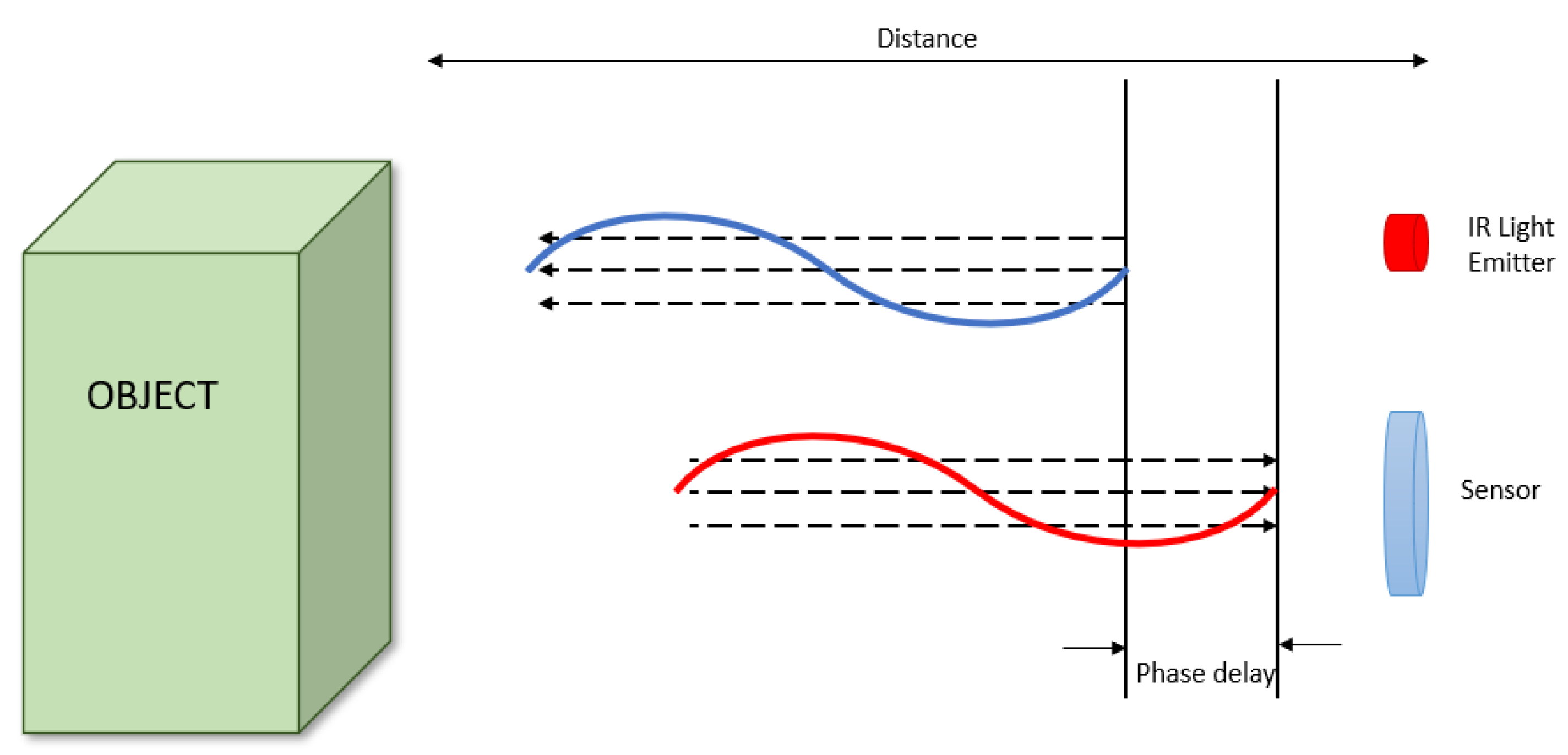
Figure 2.
Material connections.
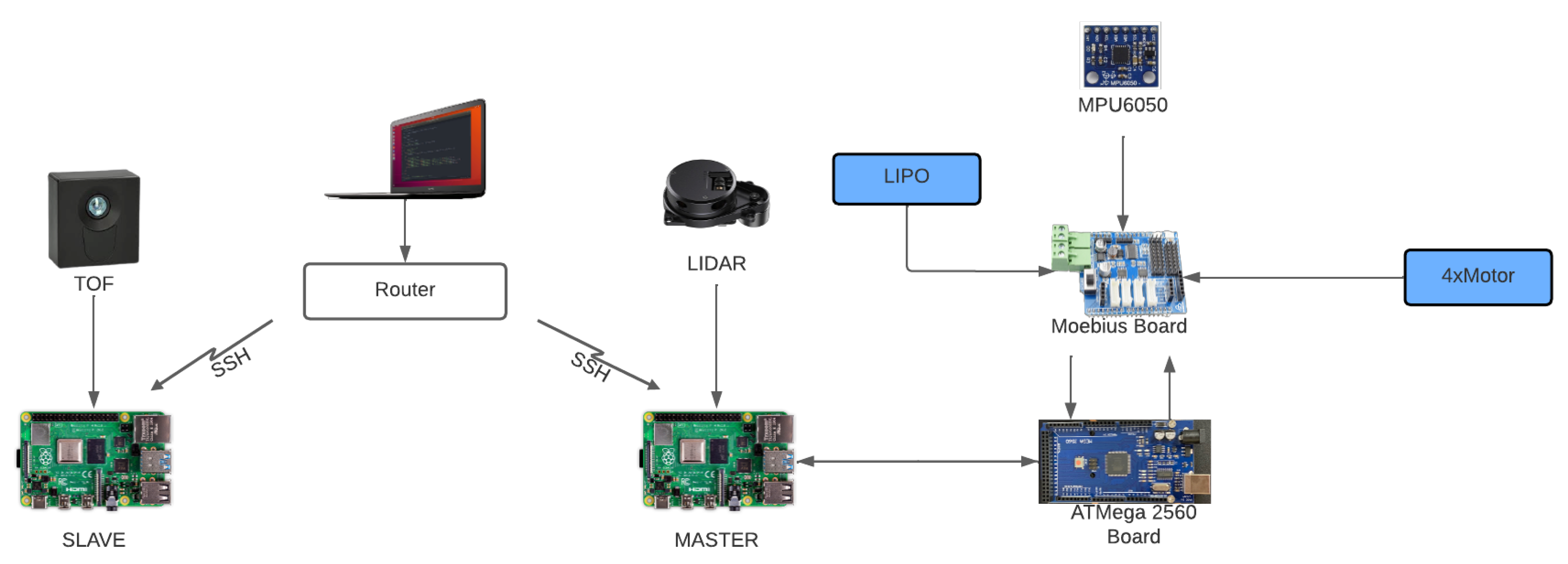
Figure 3.
The proposed methodology.
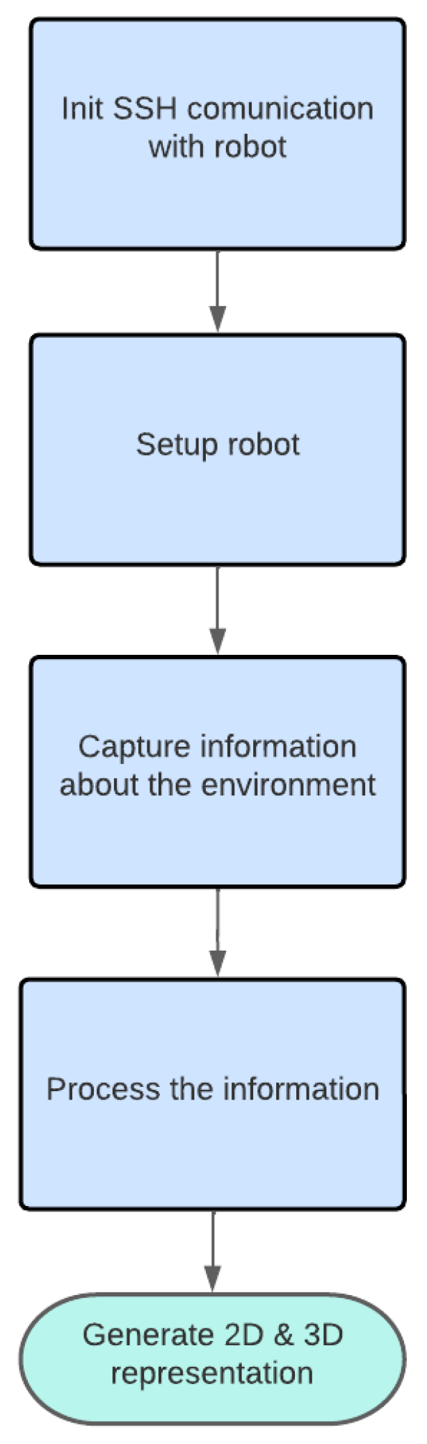
Figure 4.
Robot setup.
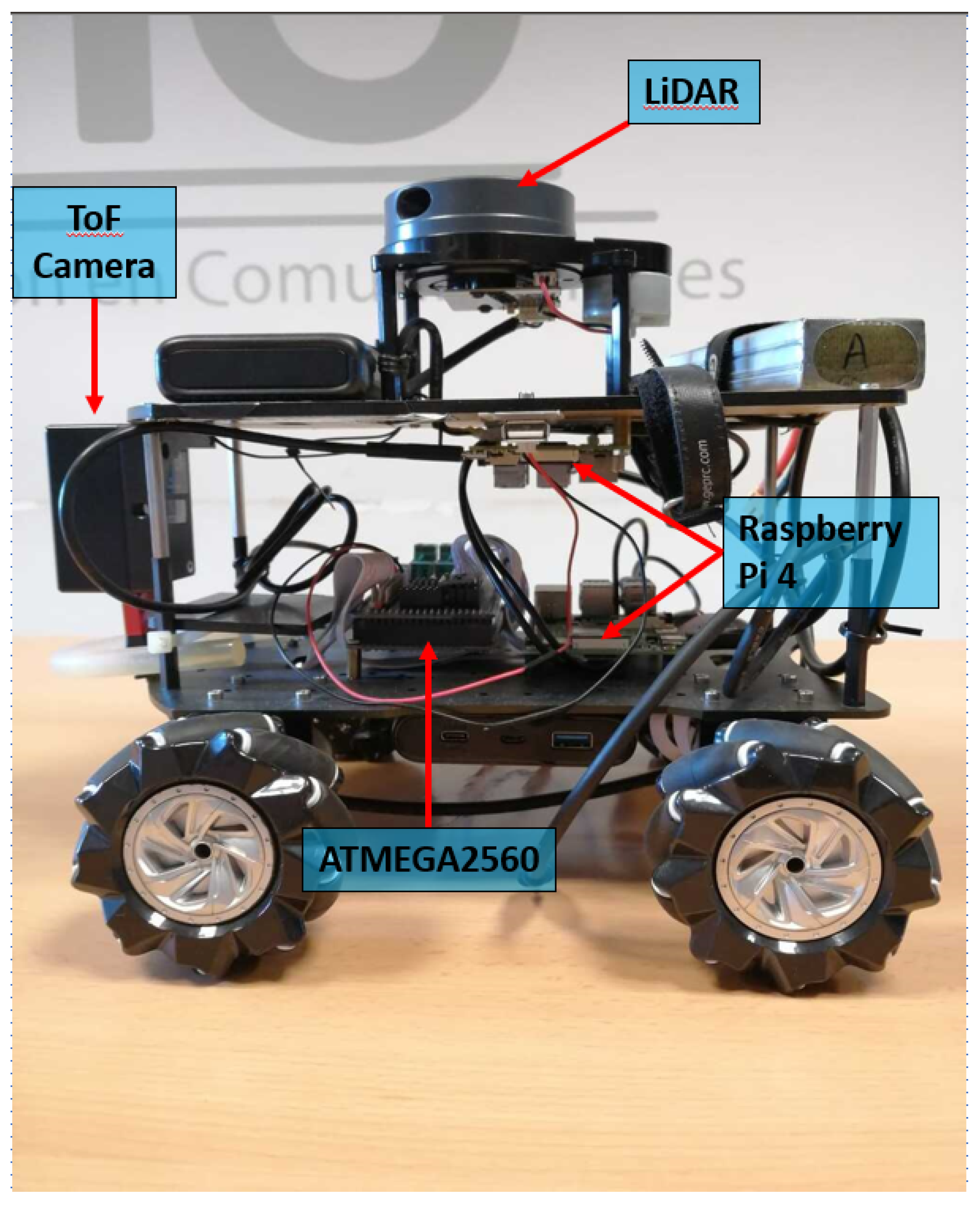
Figure 5.
Hallway representation. (a) RGB representation. (b) 2D representation.
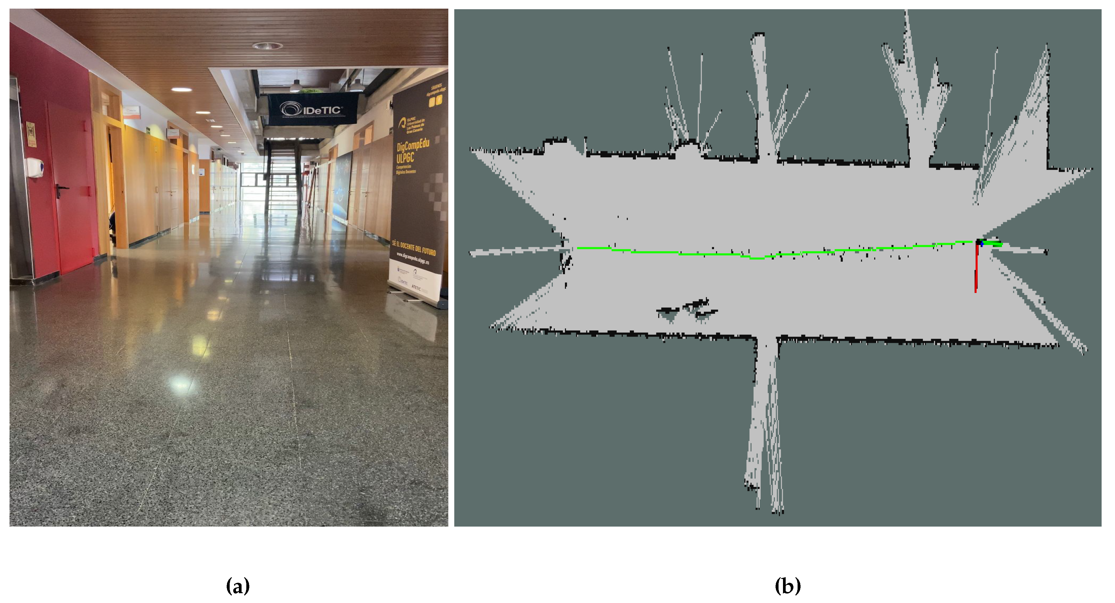
Figure 6.
2D & 3D simultaneous building.
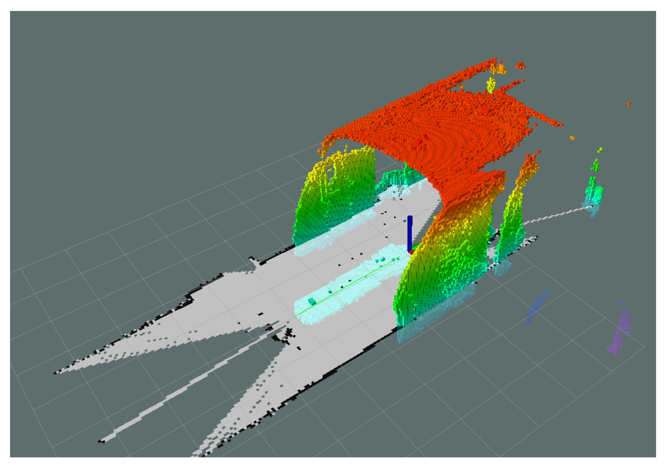
Figure 7.
3D hallway representation. (a) with roof. (b) without roof.
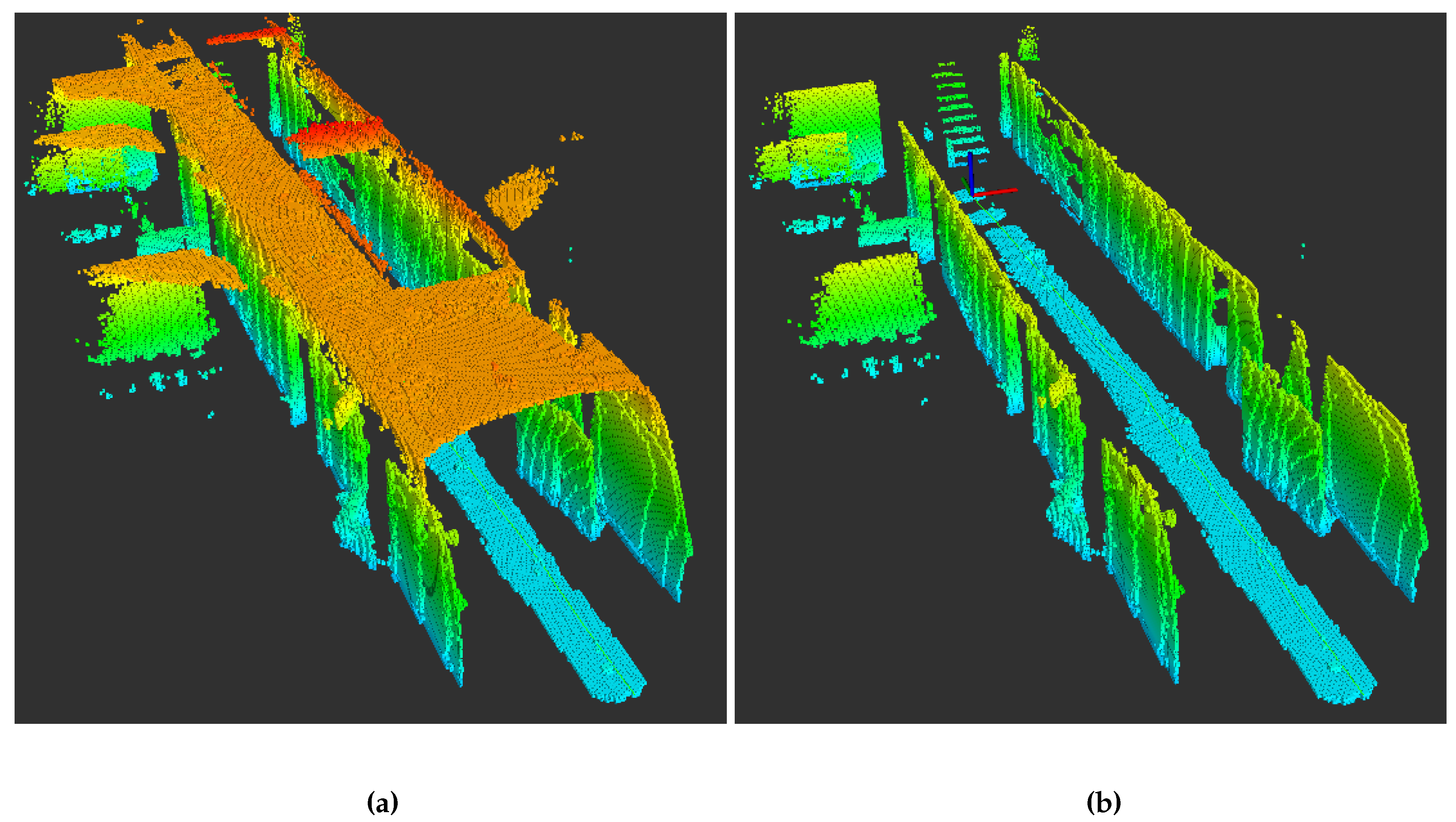
Figure 8.
Lab Room.
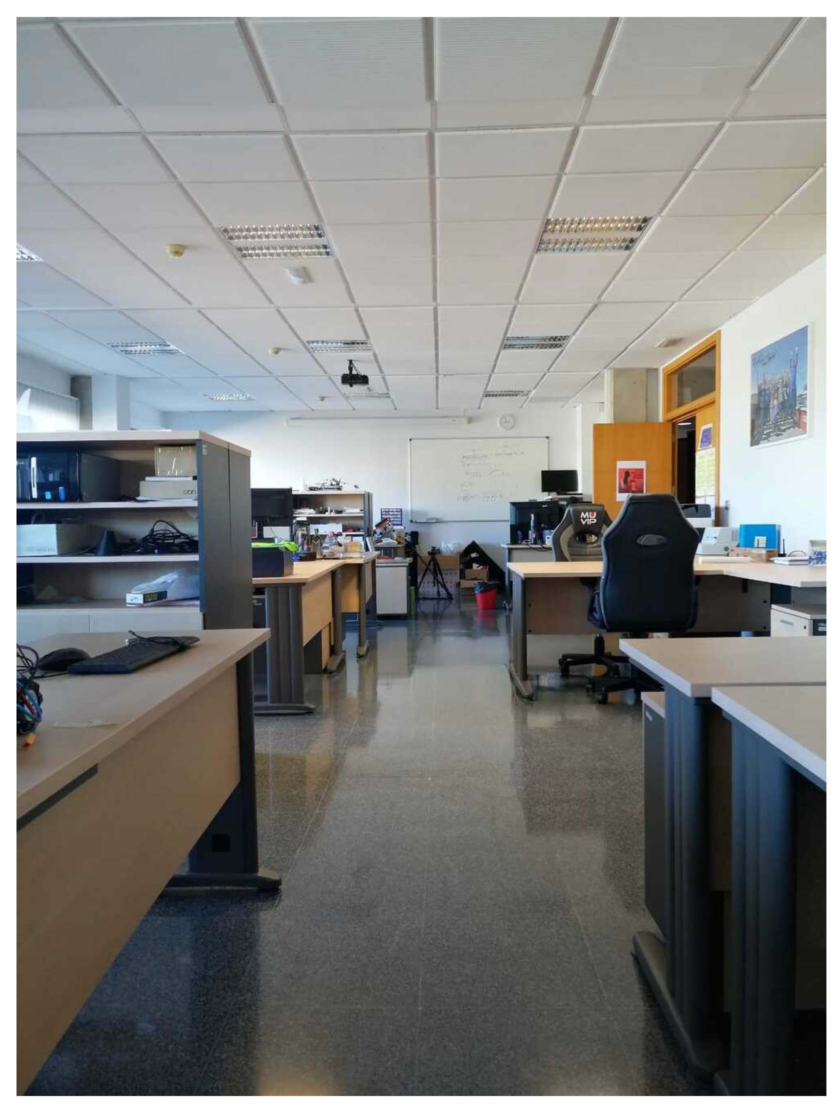
Figure 9.
Lab room representation.(a) 2D representation. (b) 3D representation.
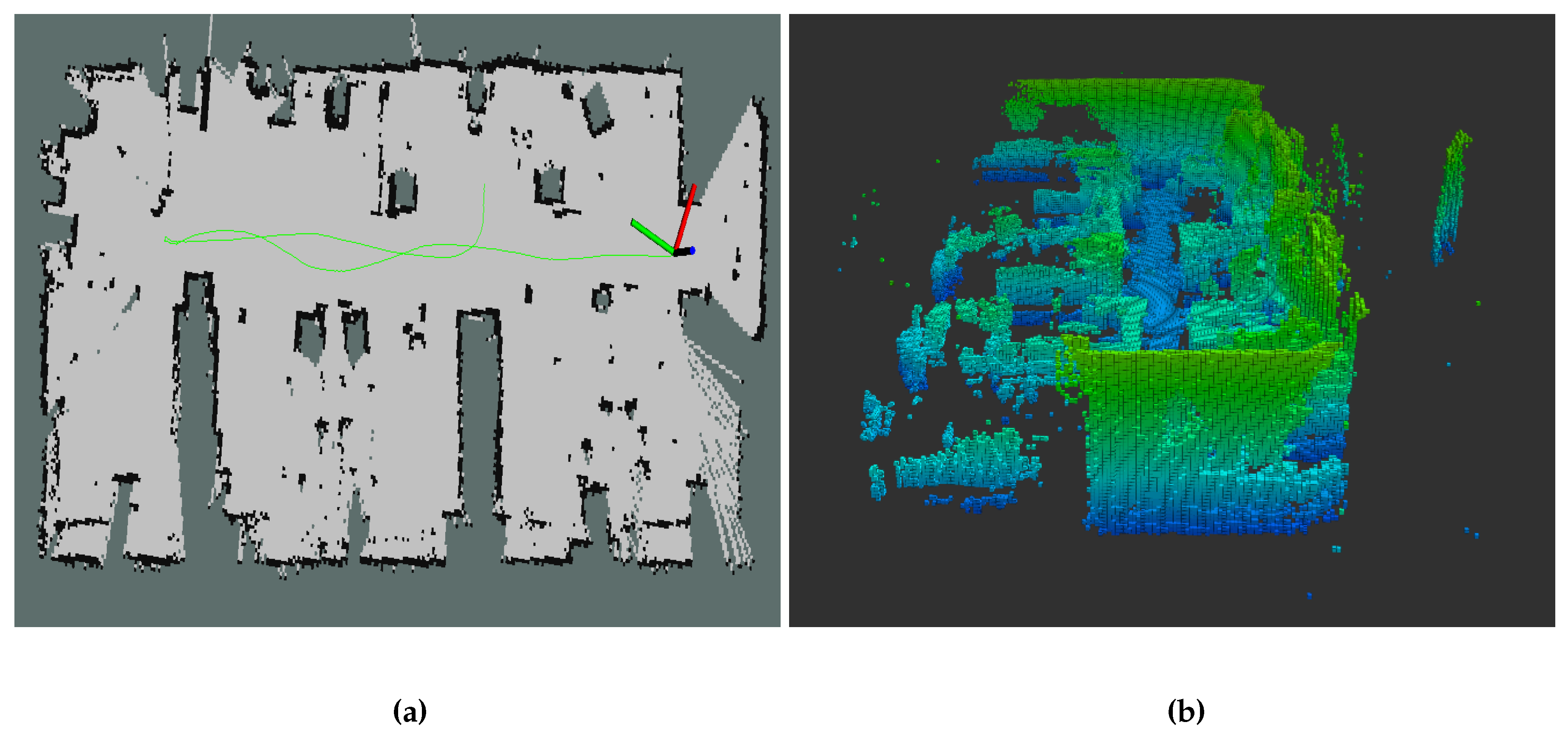
Figure 10.
Lab Room.
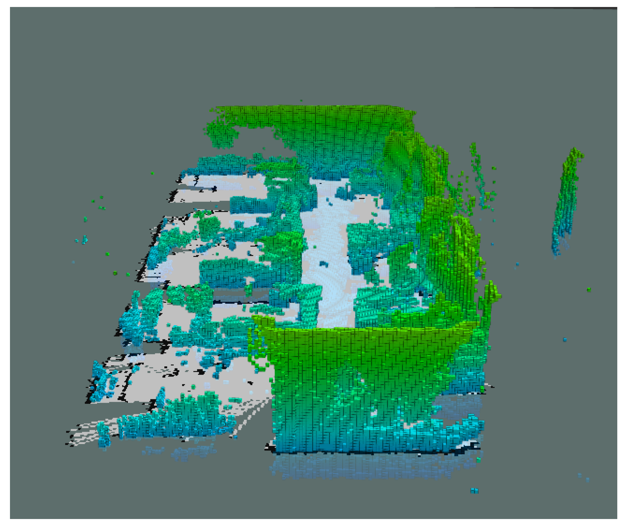

Table 1.
LiDAR characteristics.
| Range | 0.13-8m |
|---|---|
| Scanning frequency | 6.2Hz |
| Laser power | 3mW |
| Distance Variance Coefficient | DCV <0.2% |
| Voltage | 5V |
| Baud Rate | 230400 |
| Working temperature | 0ºC - 45ºC |
| Working environment humidity | <90% |
| Sampling rate | 5K/s |
| Laser wavelength | 780nm |
| Accuracy | <1%@5m |
| Communication interference | RS232 (TTL) |
| Power Consumption | 1.5W |
| Working current | 500mA |
| Level | 0º-1º |
| Working environment illumination | <1000lux |
Table 2.
ToF camera specifications.
| Measuring range | 0.5-6m |
|---|---|
| ToF Sensor | RS1125C Infineon® REAL3™ 3DImage Sensor IC based on pmd intelligence |
| Framerate | 5 fps, 10 fps, 25 fps, 35 fps, 45 fps, 60 fps (3D frames) |
| Type of light | Infrared light |
| Acquisition time per frame | 5 ms typ. at 60 fps |
| Wavelenght | 850nm |
| Illumination | 4 x VCSEL, laser class 1 |
| Viewing angle | 100º x 85º |
| Depth resolution | ≤ 1 % of distance (1-6 m at 5 fps),≤ 1 % of distance (0,5-2 m at 60 fps |
| Resolution | 352x287 (100k) pixels |
| Power consumption | USB 3.0 compliant, 4,5 W max. for IRS chip, illumination and USB 3.0 |
Table 3.
IMU characteristics.
| Supplier Device Package | 24-QFN (4x4) |
|---|---|
| Sensor Type | Accelerometer, Gyroscope, 3 Axis |
| Package | 24-VFQFN Exposed Pad |
| Output Type | I2C |
| Operating Temperature | -40°C 85°C (TA) |
Table 4.
Raspberry Pi 4 Model B characteristics.
| Processor | Broadcom BCM2711, quad-core Cortex-A72 (ARM v8) 64-bit SoC @ 1.5GHz |
|---|---|
| Memory | 4 GB LPDDR4 |
| Connectivity | 2.4 GHz and 5.0 GHz IEEE 802.11b/g/n/ac wireless LAN, Bluetooth 5.0, BLE Gigabit Ethernet 2 × USB 3.0 ports 2 × USB 2.0 ports. |
| GPIO | Standard 40-pin GPIO header |
| Input Power | 5V DC via USB-C connector (minimum 3A1) 5V DC via GPIO header (minimum 3A1) Power over Ethernet (PoE)–enabled (requires separate PoE HAT) |
| Environment | Operating temperature 0–50ºC |
Table 5.
Motor parameters.
| No-load current | 120 mA |
|---|---|
| Rated torque | 3.5 KG.CM |
| No-load speed | 330 rpm |
| Rated speed | 250 rpm |
| Rated current | 1 A |
| Maximum torque | 5 KG.CM |
| Stop current | 2.3 A |
Table 6.
Motor parameters.
| Type | AB phase incremental |
|---|---|
| encoder | 330 rpm |
| Wire speed | 360 |
| Supply power | 5 V |
| Interfaz type | PH2.0 |
| Function | Control speed |
Disclaimer/Publisher’s Note: The statements, opinions and data contained in all publications are solely those of the individual author(s) and contributor(s) and not of MDPI and/or the editor(s). MDPI and/or the editor(s) disclaim responsibility for any injury to people or property resulting from any ideas, methods, instructions or products referred to in the content. |
© 2023 by the authors. Licensee MDPI, Basel, Switzerland. This article is an open access article distributed under the terms and conditions of the Creative Commons Attribution (CC BY) license (http://creativecommons.org/licenses/by/4.0/).
Copyright: This open access article is published under a Creative Commons CC BY 4.0 license, which permit the free download, distribution, and reuse, provided that the author and preprint are cited in any reuse.


