Submitted:
17 May 2023
Posted:
19 May 2023
You are already at the latest version
Abstract
Ensuring safe and continuous autonomous navigation in long-term mobile robot applications is still challenging. To ensure a reliable representation of the current environment without the need for periodic re-mapping, updating the map is recommended. However, in case of incorrect estimation of robot pose, updating the map can lead to errors that prevent the robot localisation and jeopardize map accuracy. In this paper, we propose a safe LIDAR-based occupancy grid map updating algorithm for dynamic environments taking into account the uncertainties in the estimation of the robot’s pose. The proposed approach allows robust long-term operations as it can recover the robot’s pose, even when it gets lost, to continue the map update process providing a coherent map. Moreover, the approach is robust also to temporary changes in the map due to the presence of dynamic obstacles such as humans and other robots. Results highlighting map quality, localisation performance, and pose recovery, both in simulation and experiments, are reported.
Keywords:
Mapping
; localisation
; Dynamic environments
1. Introduction
Autonomous mobile robots are becoming increasingly popular in industrial applications such as logistics, manufacturing, and warehousing. One of the key requirements for the operation of such robots is the ability to navigate safely and efficiently in a dynamic environment, repeatedly doing the same task all day for days or months. A mobile robot’s autonomous navigation is achieved using Simultaneous Localisation and Mapping (SLAM) techniques, in which the robot maps the environment, navigates, and locates itself by merely ”looking” at this environment, without the need for additional hardware to be installed in the workplace. This is achieved by using sensor measurements (such as LIDAR, cameras, or other sensors) to update the map and estimate the robot’s pose at the same time [2]. However, these methods face significant challenges in dynamic environments, mainly when the environment changes over time due to the movement of obstacles or people. Obstacles may appear, disappear, or move around, and the robot’s map needs to be updated continuously to reflect these changes. While localisation and local obstacle avoidance algorithms can handle small changes in the environment, the robot’s map can diverge from the present working area, reducing navigation performance [3]. Conventional SLAM methods struggle to update the map accurately and efficiently over long periods of time due to the accumulation of errors in the robot’s pose estimates and in the map. This is because small errors in the robot’s pose estimation can accumulate over time, leading to significant inaccuracies in the map. Moreover, the robot needs to constantly re-localise itself, which can be challenging and time-consuming. Indeed, traditional SLAM algorithms are computationally intensive and require significant processing power, memory, and time [4]. This can limit the robot’s ability to operate for extended periods, particularly in industrial environments where robots need to operate continuously.
Therefore, the long-term operation of autonomous mobile robots in dynamic industrial environments requires continuous map updating to ensure accurate navigation and obstacle avoidance and achieve good localisation performance [5,6]. Moreover, having an updated static map, coherent with the current environment, allows the robot to reduce its effort in re-planning over time to adjust its trajectory. Updating the map in real-time requires the robot to quickly detect and track changes in the environment, such as the movement of people, equipment, and obstacles. For this reason, and in order to consider long-term operations, the map updating algorithm has to be computationally light and use limited memory [7].
In our paper [1], we proposed a 2D LIDAR-Based map updating to detect possible changes over time in the environment and to accordingly update a previously built map with limiting memory usage and neglecting the presence of highly dynamic obstacles. The system was developed using the Robot Operating System framework [8] using a 2D occupancy grid map representation. This map representation is commonly used in the industrial field due to its ability to facilitate path-planning [9,10]. In fact, companies such as AgileX RoboticsAgileX,https://global.agilex.ai/ , AvidbotsRobotnik, https://robotnik.eu/ , and BoschBosch, https://www.bosch.com/, currently employ 2D occupancy grid maps in their assets, demonstrating the technology’s high level of industrial readiness. As such, it is important to continuously improve and strengthen the robustness of this technology for long-term use.
1.1. Paper Contribution
Although the proposed map updating [1] provide promising result in map quality and localisation performance in a dynamic environment, the method relies heavily on accurate knowledge about the initial pose of the robot in a previously built map. That information might not be available with high accuracy, and due to changes in the map, it might be hard to estimate immediately. This could lead to bias in the estimated pose of the robot, which could result in overwriting free and occupied cells, effectively corrupting the occupancy grid and the resulting map. Indeed, as the robot moves through its environment, small errors in its position estimate can accumulate, resulting in a significant deviation from its true position over time. This issue is often referred to as drift and can be caused by a variety of factors, such as wheel slippage, sensor noise, and environmental changes.
To overcome this drawback and make the approach more robust, in this paper, we first introduce a fail-safe mechanism based on localisation performance to prevent erroneous map updating when the localisation error increases, and then we integrate a pose update algorithm that is activated when the robot effectively gets lost.
In our work, we propose a map updating algorithm in the presence of localisation error able to integrate localisation recovery procedures preventing degradation of the map in long-term operations. Extensive simulations have been conducted to validate the system in its components and as a whole. Finally, real-world experiments results are provided to highlight the performance of the approach in a real environment and to show its robustness in realistic uncertain conditions.
2. Related Works
Over the past few decades, an immense and comprehensive body of research has emerged regarding the issue of updating maps in a dynamic environment to support long-term operations. Sometimes, the researchers refer to the problem as a lifelong mapping or a lifelong SLAM one. In this section, we present the most relevant solutions proposed in the literature related to the occupancy grid map representation and methods for updating an existing one, going to underline the difference with conventional slam methods.
2.1. Occupancy grid
Occupancy grid maps are a spatial representation that captures the occupancy state of an environment by dividing it into a grid of cells. Each cell is associated with a binary random variable indicating the probability that the cell is occupied (free, occupied, or unknown). One common method for updating the occupancy grid map is to use a probabilistic model such as the Bayesian filter [11]. This filter estimates the probability distribution of the occupancy state of each cell based on the likelihood of sensor measurements and the prior occupancy state. Most occupancy grid map algorithms derive from the Bayesian filters and differ from the posterior calculation. However, the Bayesian approach has drawbacks in the difficulty of correct map updates based on possible uncertainties in the robot poses, [12]. Although the construction of a static environment map using the occupancy grid approach has already been solved [13], its effectiveness in dynamic environments over extended periods of time still requires further investigation. Different methods have expanded the occupancy grid map algorithms to handle dynamic and semi-static environments [14,15,16,17]. These approaches assess the occupancy of cells irrespective of the type of detected obstacle, thereby mitigating the challenges related to multi-obstacle detection and tracking and improving the speed of the mapping process [18]. However, their primary focus is on accelerating the mapping construction process rather than in the updating process of an initial occupancy grid map for an extended period of time. This may limit the use of such approaches in, possibly large, industrial scenarios where a full map reconstruction requires a computational and resources effort to replan continuously the whole robot motion in the new map.
2.2. Lifelong Mapping
In the literature, there exist grid-based methods aimed at lifelong mapping. One group of these algorithms is based on the update of local maps, as demonstrated in [7], based on a weighted recency averaging technique to detect persistent variations. They merge these maps using Hough Transformation. However, this approach assumes that no dynamic obstacles are in the environment. In contrast, [19] still generates local maps and continuously update them online requiring a substantial memory usage. To address this, [20] proposed pruning redundant local maps to reduce computational costs while maintaining both efficiency and consistency. However, these systems are not currently used in industrial applications, except for closed navigation systems, and are not comparable with occupancy grid-based methods like the one proposed in this paper because the map representation they rely on is different. Instead, in [6] the authors update a 2D occupancy map of a non-static facility logistics environment using a multi-robot system, where the local temporary maps built by each robot are merged into the current global one. While the approach is promising for map updating of non-static environments, the need for precise localisation and assumptions on the environment can be challenging in cluttered and dynamic environments, providing a limit of the method.
2.3. Lifelong Localisation
In order to perform long-term operations in a dynamic environment, the map used by the robot to autonomously navigate needs to be up-to-date and accurately reflect the current state of the environment. To update a map correctly, a robot must first accurately localise itself within the environment. If the robot’s position is incorrect or uncertain, any updates made to the map may be inaccurate, leading to errors in navigation and task performance. In the literature, there are several works that take into account the localisation problem in order to achieve better results in the map update process which, like our proposed approach, does not fall within SLAM systems. In [21], the author proposed a method for the long-term localisation of mobile robots in dynamic environments using time series map prediction. They produce a map of the environment and predict the changes in the 2D occupancy grid map over time using the ARMA time series model. The robot’s localisation is then estimated by matching its sensor readings to the predicted map. The proposed method achieves better localisation accuracy and consistency compared to traditional methods that rely on static maps. However, there are some limitations related to the computational complexity of the time series model, which can make real-time implementation challenging. Additionally, the accuracy of the map prediction is highly dependent on the quality of the sensor data and the ability of the time series model to accurately capture the dynamics of the environment. In [22], Sun et al. proposed an approach for achieving effective localisation of mobile robots in dynamic environments. They solve the localisation problem through a particle filter and scan matching. When the matching score is above a certain threshold, the map updating step is performed. However, they consider only environments with a clearly defined static structure. In [23], instead, they discourage map updating if the robot is in an area with low localisability (i.e. the map is locally poor in environmental features). To further improve robustness, they introduce a dynamic factor to regulate how easily a map cell changes its state. Although they do not make any explicit assumption on the environment, the dynamic factor works well in scenarios where the changes occur regularly (e.g. a parking lot, where the walls are fixed, and the parking spots change occupancy state frequently). Instead, it is not well-suited for environments that slowly change in an irregular and unpredictable fashion. All the works mentioned above follow the same pattern, on which we took inspiration for our approach, starting from a previously created map and applying various methods to ensure a robust localisation that leads to a correct map update. However, all of them do not provide results concerning the robot lost localisation case. On the contrary, our approach does not provide a continuous localisation algorithm but an evaluation of the localisation error so as not to update the map incorrectly. Finally, our approach handle also the case of a robot get lost in the environment due to localisation errors.
2.4. Conventional Lifelong SLAM
Other systems that try to solve autonomous navigation in long-term operations rely on lifelong SLAM. In such scenarios, the SLAM technique is used to provide either a new map every time the robot performs a new run or an updated map, both robust to localisation error and environmental dynamics. Thus, they are oriented to reduce e.g. computational performance, loop closure, and pose graph sparsification [4], resulting in a stand-alone system based on internal structure that can not be straightforwardly integrated and hence easily used in industrial systems. This is also due to the fact that they may be not based on occupation grid map approaches. In the paper [24], for example, the authors present a new technique based on a probabilistic feature persistence model to predict the state of the obstacles in the environment and update the world representation accordingly. [25], on the other hand, approaches each cell’s occupancy as a failure analysis problem and contributes temporal persistence modeling (TPM), which is an algorithm for probabilistic prediction of a cell’s "occupied" or "empty" state given sparse prior observations from a task-specific mobile robot. Although the introduced concept is interesting, it suffers from the limitation due to temporary map building for motion planning and hence it does not provide an entire updated representation of the environment.
Due to their incremental approach, most life-long SLAM available systems rely on graphs, [26,27], or other internal structures. Even if an occupancy grid map can be built for navigation purposes, an existing graph structure is required as input rather than a previous occupancy grid map.
Finally, our intent and difference with a slam method should be clear. Our proposed approach is based on the localisation error evaluation of the robot’s estimated pose provided by any localisation algorithm to update the map correctly and continue its update in case of loss of the robot’s pose. The proposed approach is proven to be able to capture environmental changes while neglecting the presence of moving obstacles such as humans or other robots. Moreover, the approach is designed to guarantee limited memory usage and to be possibly and easily integrated into typical industrial mobile systems.
3. Problem Formulation
Consider a mobile robot , represented by with and be the robot position and orientation, is equipped with a 2D lidar and encoders and operates in a dynamic environment . To navigate autonomously, requires a map and a generic localisation algorithm that provides an estimate global robot pose , where and are the robot estimated position and orientation, such that the localisation error is smaller than a threshold to allow the robot completing its task. In the case of dynamic environments, the arrangement of the obstacles present in the environment changes in time, effectively creating new environments with that are similar to the precedent ones . What happens is that over time a static map no longer reflects the current configuration of leading to localisation errors hence degrading the operational performance of . One solution is to provide a map that is updated over time to reflect , and such that .
Occupancy Grid Map: In this paper, we consider the occupancy grids technique to represent and model the environment in which the robot operates. A 2D occupancy grid map is a grid that represents the space around the robot through cells that contains information about the area associated with its position in the space. Each cell in the grid represents the probability of the cell being occupied by an obstacle (probability equal to 1, black cells in Figure 1), free (probability equal to 0, grey cells in Figure 1), or unknown (otherwise, dark grey cells in Figure 1).
Figure 1 shows the 2D occupancy grid map representation considered in this paper for a map of 8x8 cells. The map’s cells are identified through the grid coordinates that define the actual resolution r of the occupancy grid and the finite locations of obstacles. The origin of grid coordinates is in the bottom-left corner of the grid, with the first location having an index of (0,0). Given the 2D occupancy grid map, the cell identified by a point has the following grid coordinates:
There are several sensors that can be used to build 2D occupancy grid maps such as Lidars, cameras, sonar, infrared sensors, etc…, but in our work, we considered only 2D Lidars to generate a 2D point cloud. It is worth noting that our method is also suitable for any sensors able to provide this kind of information.
Lidar Point Cloud: Given a laser range measurement with n laser beams at time k, it is possible to transform the data in a point cloud , where is the i-th hit point at time step k, i.e. the point in which the i-th beam hit an obstacle. Moreover, given and the estimated robot’s pose , it is possible to obtain the coordinates of in a fixed frame asto ease the notation, the time dependence k is omitted:
where with we represent the cartesian coordinates of the hit point along the i-th laser range measurement . The angular offset of the first laser beam with respect to the orientation of the laser scanner is represented by considering that the angular rate between adjacent beams is . Finally, given the set of cells passed through by the measurement is where is the cell associated to .
3.1. Ideal Scenario Vs Real Scenario
Given a mobile base , equipped with a 2D lidar, operating in an environment represented by a 2D occupancy grid map, the ideal simplified scenario is depicted in Figure 2: a laser beam hits an obstacle in a cell that is occupied, and it is identified as the only cell selected by the laser measurement thanks to an accurate knowledge of the robot pose.
However, the real scenario presents a different situation, depicted in Figure 3. Since there are localisation errors, the robot’s pose is affected by uncertainty, represented in the figure by the green cells around the robot. The localisation error and the addition of measurement errors and noises lead to the possibility that a laser beam may not identify the correct cell but another one in its neighborhood (green cells around ). For this reason, a direct check on the occupancy of the identified cell may lead to errors in the map update process. Hence, a procedure that is robust with respect to such localisation and measurement errors and noises must be developed.
4. Method
The proposed system architecture is represented in Figure 4, where based on an initially provided occupancy grid map , the robot pose provided by any localisation algorithm, and the current laser measurements , our approach computes a newly updated map and a new robot pose accordingly to the localisation error. Indeed, as shown in Figure 5, only state of the cells that correspond to relevant changes in the environment are updated in case the localisation error is limited. Otherwise, the map updating process is suspended until the localisation algorithm recovers the right estimated pose. If the latter is not able to provide a new and the drift accumulation is too big, a pose updating process is activated to estimate a new robot pose.
To evaluate the localisation error, we first classify with the Beams Classifier the laser measurement as either “detected change measurement” or “non-detected change measurement”, this characterization is computed checking for discrepancy of the measurements with the initial map as described in Section 4.1. Then, the detected change measurements are evaluated by the Localisation Check as described in Section 4.2 to assess the localisation error. If the error is small enough, the map updating process can continue. Otherwise, the system stores the last updated map and the correct and continues to monitor the localisation error, pausing the map update process. If the error continues to increase, the pose updating process is activated to provide a new based on , , and . The map updating process, depicted in Figure 6, is responsible of the detection of changes in static obstacles (i.e., removal or addition) while it neglects the possible presence of dynamic obstacles in the environment that can lead to a corrupted map, e.g. people or other robots. If the Localisation Check is successful, it means that the localisation error is limited and hence the outputs of the Beam Classifier together with and are used by the Changed Cells Evaluator and the Unchanged Cells Evaluator to evaluate possible changes in the cells associated with current measurements with respect to the initial map . Confirmation procedures are necessary to address the localisation errors, even if limited, and possible noises that can affect the information retrieved by measurements. To simplify detection, all unknown cells in are considered occupied during the measurement process to reduce to two the possible type of cell’s states. A rolling buffer of a fixed size is created for each cell , and to record the outcomes of the evaluator blocks at different time instants. The Changed Cells Evaluator fills with a "changed" flag only if the associated measurement is classified as "detected" and the change is confirmed as described in Section 4.3. The Unchanged Cells Evaluator fills with an "unchanged" flag only if the associated measurement is classified as "non-detected" and the evaluation is confirmed as described in Section 4.4. In the end, the Cell Update module changed between free and occupied the state of evaluated cells only if a sufficiently large amount of "changed" flags are in the associated buffer , as described in Section 4.5. This module is the one responsible for the detection of changes in the environment while neglecting dynamic obstacles.
4.1. Beam Classifier
To detect a change in the environment, the outcomes of measurement must be compared to the ones the robot would obtain if it were in an environment fully corresponding to what memorized in map . The correct hit point as in (2) is hence compared to the one computed with that is the expected value for the i-th range measurement obtained from the initial map . A ray casting approach, [28], is hence used to compute the corresponding expected hit point :
To detect a change, we do not directly compare the measured hit point with the expected hit one . Indeed, we use a 1-to-N comparison strategy with a set of expected hit points consisting of hit points along virtual neighbouring range measurements.
Note that (3) computes the expected hit point as the sum of an offset and a point with polar coordinates , the set is generated by adding different perturbations v to the angular second point. More in detail, the set of points is generated by adding a perturbation v to the angular components of in (3):
where l is integer and , while and are design parameters. The distance is defined, in an analogous way as , as the measurement in along the virtual laser ray of amplitude with respect to the i-th real ray. Note that, v is chosen so that perturbations , and hence between the -th and the -th laser rays. An example of , and hence, is reported in Figure 7).
For the 1-to-N comparison, each point is compared to the entire set by computing the minimum Euclidean distance between and the N points in . Finally, a change is detected only if the minimum distance between and the expected points in is greater than a threshold :
As described in detail in Appendix A.1, the threshold can depend linearly on the distance in order to take into account errors coming from localisation and measurement noises.
The motivation for the 1-to-N comparison is represented in Figure 8: the removal of an obstacle (in red) creates a change in a portion of the map, and a false change detection associated with the hit point computation may occur. Figure 8 shows the hit point identifying a cell of the new map that has not changed compared to the previous map . On the other hand, small localisation errors may lead to an associated identifying an occupied cell belonging to the obstacle in . A direct comparison between and creates an incorrect change detection. This does not happen in Figure 8, where thanks to the 1-to-N comparison with the set the presence of a close to prevent the incorrect change detection.
4.2. Localisation Check
Changes in the map may have two drawbacks, first, they may prevent the robot from correctly localising itself in the changed map, second, as a consequence, large localisation errors may lead to an incorrect update of the map. Hence, monitoring the amount of localisation error is fundamental for a correct map update. For this purpose, the proposed dedicated Localisation Check module takes in input all the "detected change" measurements from the Beam Classifier and provides a quantification of the current localisation error. This module is important to make more robust the entire system by preventing corrupted maps update and by triggering a pose updating algorithm to decrease the localisation error. The idea is to evaluate the amount of localisation error and until this is below a given threshold the map can be updated neglecting the error. On the other hand, if it is too large, the robot is considered to be definitely lost and a pose update is requested to a dedicated algorithm. On the other hand, in between those two extreme cases and thresholds, it is possible to have a sufficiently large localisation error that would provide a corrupted map update but not so large to consider the robot definitely lost. In this case, the map update is interrupted and restarted once the localisation error decreases below the corresponding threshold.
More formally, given the number n of hit points in , derived from laser measurement , and the number of the "detected change" measurements, the map is updated as described next if
while the robot is considered lost but with the possibility of recovering the localisation and the map is not updated, if the following holds:
Finally, the localisation system is considered not able to recover the pose and this must be updated by a dedicated algorithm if
where is the minimum fraction of acceptable changed measurements with respect to the number of laser beams that allows a good localisation performance, while is the maximum fraction of acceptable changed measurements with respect to the number of laser beams in addition to which the robot has definitively lost its localisation. The critical parameter to choose is because it is a trade-off between the great change between the previous and current environments and the likelihood that you have actually lost your localisation. In this paper, the values and are considered based on the results of several experimental tests.
4.3. Changed Cells Evaluator
Let represents the occupancy state of a cell in the initial map . Once a change is detected by the Beam classifier along the i-th range measurement , it is necessary to evaluate whose states of cells in must be modified, i.e. the cells passed through by i-th laser ray. The Changed cells evaluator is the module that determines which are the cells in involved in the detected change. Once a change is confirmed in a cell, the module stores a “changed” flag in the buffer of each cell. The status of a cell will be changed based on how many “changed” flags are in its buffer at the end of the procedure, as described in Section 4.5. The two possible events that cause a change in the environment are illustrated in Figure 9: the appearance of a new obstacle (Figure 9) and the removal of an existing one (Figure 9). A combination of these two events may also occur (Figure 9). The following paragraphs will describe how the cells in , i.e. along the beam, are checked by the Changed cells evaluator module in the occurrence of such events. A distinction between the cell and all other cells along the ray, i.e. , is necessary for the evaluation as described next.
4.3.1. Change detection of cells in
A first evaluation is conducted on the cells along the ray, except for that corresponds to the hit point . Indeed, all those cells should have a free status, since they correspond to points of the laser beam that are not hit points. To increase algorithm robustness, we choose to not modify the status of the cells corresponding to the laser beam final chunk, since such cells may correspond to points that actually lay on obstacles due to localisation errors. For this reason, only cells between the robot’s estimated position and a point that lay on the laser beam (i.e. on the segment with extremes and ) are evaluated, see Figure 10. More formally, given a fixed parameter and , we analyse only the cells that satisfy:
where is the point in the centre of the cell . If a cell satisfies (9) with it means that an obstacle has been removed with respect to and a “changed” flag is hence added to the cell’s buffer to report this change.
4.3.2. Change detection of
The status of must also be evaluated. However, in this case, the events of a newly added obstacle and of a removed one must be distinguished. Indeed, in an ideal situation, when a new obstacle is added the hit point lies on the new obstacle, and hence its associated cell has a free status in , and hence it should be changed to occupied, see Figure 11. On the other hand, when an obstacle is removed, the hit point lies on another obstacle or part of the environment hence its associated cell has an occupied status in , and hence it should not be changed, see Figure 11.
Unfortunately, in case of localisation errors it may occur that the (not ideally computed) cell corresponding to the measured hit point may be free in both cases of added or removed obstacles, see Figure 12. Hence, in case of localisation errors, the distinction among added or removed obstacles is not possible with a direct evaluation of single-cell occupancy. On the other hand, in case of added obstacle also all cells sufficiently close to are free in while in case of a removed one some of those cells would be occupied and hence a distinction between the two cases is possible if closed cells status are also checked, see Figure 13.
To conclude, a new "changed" flag is effectively added to the buffer of if the added obstacle is detected, i.e. the state of neighbouring cells is free, more formally if:
where is a point in the space and is a function of the measured range as in (5).
4.4. Unchanged Cells Evaluator
In case the Beam Classifier does not detect changes along the i-th range measurement , none of the maps cells associated with has undergone any changes with respect to the initial map . To take into account localisation errors, a similar procedure to the one described in the previous section can be applied, and only cells between the robot’s estimated position and the point that lay on the laser beam are evaluated. In particular, for such cells, the Unchanged Cells Evaluator add an “unchanged” flag to their buffer. Also for cell localisation errors must be taken into account. Indeed, since the Beams Classifier did not detect any change, the status of cell should be occupied in map but localisation and noise errors may lead to a measured hit point with associated free cell and nearby occupied cells. Therefore, if , an “unchanged” flag is added to the buffers of all occupied cells adjacent to . Otherwise, an “unchanged” flag is added only to the buffer of .
4.5. Cells Update
Once each ray has been processed by the Beam classifier and cells along the ray have been evaluated by the two previously described modules, the Cells Updating module is responsible for updating/changing the state of each cell in for all measurements with an update rate that depends on both linear and angular speed of the robot. For each cell , this update is based on the occurrence of “changed” flags in the corresponding buffer . Let denote the size of the rolling buffers, and let count the occurrences of the “changed” flag in . A cell’s occupancy state is changed only if exceeds a given threshold, which balances the likelihood of false positives with the speed of map updates and change detection. This threshold, and itself, are critical parameters; the threshold is used to make the cell updated status more robust with respect to dynamic events in the environment while represents the memory of past measurements. Indeed, with a good balance in the choice of such parameters, using this approach, highly dynamic obstacles are initially detected as changes in measurements but discarded during cell update if there is an insufficient number of “changed” flags in the corresponding buffer, and hence are not considered in the new map .
It is worth noting, that a change of cell state from occupied to free can lead to a partial removal of an obstacle. Referring to Figure 14, cells corresponding to the border of an obstacle can hence be set as free leading to an updated map with obstacles without borders characterized by measurable cells with unknown state, see Figure 14 where black cells are occupied while red ones are unknown. To avoid this, the state of those cells must be set to occupied, leading to the creation of the new border as in Figure 14. At this point, the cell state update procedure is finished, and the new map can be created. To do so, it is important to recall that cells in the initial map with “unknown” state have been considered, and treated, as occupied cells in the Beam Classifier module. However, if their state has not been changed to occupied to recreate an obstacle border, they are represented in still as “unknown” cells.
4.6. Pose Updating
The Pose Updating module is activated when the Localisation Check one detects that the robot is lost with no possibility to recover its pose. To avoid possible collisions, when the localisation error is too high, the robot is stopped until the end of the pose updating process.
The module takes as input: the last estimated pose of the localisation algorithm , the last updated map , and the current laser measurement . To retrieve the robot pose, the idea is to compare what the robot currently sees, i.e. the laser measurements , with what it would see if it were in the last correctly estimated pose , i.e. the expected point cloud computed from the last updated map from the estimated pose. Practically, the Pose updating module estimates the rigid transformation between the point cloud , obtained from , and the point cloud , computed from map in the last correct pose . To compute , we used the same approach as in Section 4.1, while to estimate it is possible to apply any methods that can be used to find a rigid transformation between two point clouds, e.g. Iterative Closest Point [29], or Coherent Point Drift [30].
5. Experiments and simulations
Results of simulations and experimental data of the proposed approach are now reported. First, we present a simulation example of how the localisation check module works in case condition (7) occurs, and therefore the map update is suspended. Then, we show the reason why this mechanism is important by comparing our new approach with our previous one [1] in a simulation example.
Subsequently, we provide a numerical validation carried out in a hundred simulation scenarios by giving a quantitative performance evaluation of the system in terms of map quality and localisation improvement. We compare the updated computed maps with their corresponding ground-truth ones based on quantitative metrics. Moreover, localisation accuracy with and without our updated maps are analysed through the Evo Python Package[31] and the uncertain covariance matrix associated with the estimated pose. Next, we present how the pose update module works in simulation confirming the robustness of the method, and in the end, we report the results performed during experiments in a real-world environment.
The code developed for the experiments is available at
https://github.com/CentroEPiaggio/safe_and_robust_lidar_map_updating.git, while the videos of the reported experiments are available in the multimedia material and at this linkhttps://drive.google.com/drive/folders/1Uwa3lXIQeyXnNTykkr46e6xlvpJbzlXD?usp=share_link.
5.1. Map benchmarking metrics
To evaluate the quality of our updated map with respect to the ground-truth ones, we adopt, as in [1], three metrics, reported here for reader convenience. All the ground-truth maps were built using the ROS Slam Toolbox package [32].
Let and be the occupancy probability of the cells that contain the point q in the maps M and, respectively. Furthermore, let the number of cells in the maps, and
1) Cross-correlation (CC). The Cross-correlation metric measures the similarity between two maps based on means of occupancy probabilities of the cells and is given by:
2) Map score (MS). The Map score metric compares two maps on a cell-by-cell basis:
taking into account only cells that are occupied in at least one map to avoid favouring the map with large free space.
3) Occupied Picture-Distance-Function (OPDF). The Occupied Picture-Distance-Function metric compares the cells of a map M to the neighbourhood of the corresponding cells in the other map and vice versa. The Occupied Picture-Distance-Function can be computed as:
where is the number of occupied map cells in M, is the minimum between the search space amplitude r (e.g., a rectangle of width w and height h, ) and the Manhattan-distance of each occupied cell of the first map M to the closest occupied cell on the second map . Since the function in (11) is not symmetric, we consider the average of the OPDF distance function from M to and from to M as follows:
5.2. Experiments and Examples Procedure
All the experiments and examples conducted follow the same procedure:
- 1.
- The robot is immersed in an initial world, usually denoted with , and it is teleoperated to build an initial static map through the ROS Slam Toolbox package. Given the proposed map update procedure starts from 2.
- 2.
- The world is changed to create similar to the previous world .
- 3.
- The robot autonomously navigates in the new environment by localising itself with the Adaptive Monte Carlo Localisation (AMCL) [33] using the previous static map , while our approach provides a new updated map .
- 4.
- Increase i by one and restart from 2.
For all the world created with , a ground-truth map is built for the map quality comparison.
5.3. Simulation Environment
The laptop utilized for the simulations had an Intel Core i7-10750H CPU, 16 GB of RAM, and Ubuntu 18.04 as the operating system. To simulate a 290 square meter industrial warehouse, we employed models from Amazon Web Services Robotics [34]. These models were employed within the Gazebo simulator [35]. The specific robot used in the simulation was the Robotnik XL-Steel platform, which was equipped with two SICK s300 lidarsRobotnik xl-steel simulator, https://github.com/RobotnikAutomation/summit_xl_sim.
5.3.1. Localisation Check
The goal of the first simulation is to show how the procedure described in Section 4.2, for which the map update system is suspended due to excessive localisation errors, works. Let the robot operates in a world localising itself based on the map built while navigating in the previous world , and let the proposed algorithm updates the static map to provide . Simulations are reported for the world reported in Figure 15 with the corresponding built map in Figure 15. In this case, we suppose that the map has been built correctly and hence it can be considered as a ground-truth map, i.e., . The changed worlds and its ground-truth map are reported in Figure 15 and Figure 15 respectively, where green circles are the added obstacles and red circles are the removed ones.
The system evolution is reported in Figure where the map update and the position of the robot in the world are reported at different time instants. In Figure 16 and Figure 16 the robot is immersed in the world with while the localisation filter use the map to localise the robot with an initial estimated pose . In Figure 16 we can see: our initial updated map, , the robot in with the particles of the localisation filter represented as red arrows close to the robot and the laser measurement as red points. Observing Figure 16, it is possible to state that the robot is not localised correctly also because part of the laser measurements does not overlap with the edges of the map (see e.g. the laser beams indicated by the blue arrow). However, the presence of a part of the measurements overlapping the map edges correctly (indicated by the yellow arrow), suggests that the localisation system can still recover the pose. Under these conditions, the localisation check module suspends the map update, and the localisation error is kept monitored. Figure 16 and Figure 16 represent the system after around 10 seconds: the localisation error is reduced as expected, and this is deduced by the fact that the laser beams at the top left of the map start to overlap the borders. However, the localisation error is still in the boundaries in (7), and hence the map updating is still prevented. After 20 seconds, the situation is represented in Figures and , where the localisation system has recovered the right pose of the robot, and the map updating process has been started. Indeed, the robot recognizes that boxes in ellipses A, C, and E (in Figure 15) have been removed and part of the corresponding cells have been set to free (light gray in the figure). On the other hand, laser measurements (red points) are detecting the presence of boxes in ellipses B, D, and F (in Figure 15). Finally, the algorithm proceeds for another 40 seconds with the map updating module working properly. The situation is represented in Figures and where the previously detected left border of box B has been added to the map (cells in black).
To fully understand the necessity of such interruption in the map update process, we provide the comparison results of our old approach [1] (where the map was always updated) with the one proposed in this paper with an initial localisation error. The comparison is performed in the scenario reported in Figure 17: the first environment is in Figure 17, while the robot’s operating in world , Figure 17. The ground-truth map of used for the comparison results is reported in Figure 20.
In this example, the robot is navigating in the world , the localisation algorithm will use to provide the global estimated robot pose while both approaches will update the map providing . As can be deduced from the red arrows and the not overlapping measurements with map borders in Figure 18, we intentionally mis-initialised the localisation filter with an error around . The robot will move in a straight line until the localisation algorithm recovers the right pose.
In the left column of Figure , we provide the updated map computed using the approach in [1] during the robot navigation. On the other hand, in the right column of Figure the maps created with the proposed approach are reported.
The final maps obtained from the two approaches are shown in Figure 20. From a qualitative point of view, we can note that our old approach provides a wrong updated map compared to the ground-truth one of Figure 20. Indeed, the method wrongly changed the status of some cells belonging to the walls and correctly updated the status of some cells, highlighted in yellow, but in a wrong position, as we can see comparing Figure 20 and . Instead, our new approach has started to update the map later, but the resulting map is more precise.
Furthermore, to quantify the increase in map quality with our new approach, we applied the metrics described in Section 5.1 in order to compare the two updated maps with the reference ground-truth . The results are in Table 1 where a score is a full correspondence of the two maps. It is worth noting that not updating the obstacles’ internal cells affects the first two metrics, but not the third, which reports more accurate results. For each metric, the percentage value for the procedure proposed in previous work and the one introduced here with the localisation check module is reported. The updated map provided by our new approach with the localisation check module has, for each metric, a higher percentage value with respect to the one built without that module when compared with the ground-truth map, and this motivates the need for such module.
5.3.2. Numerical Validation
To validate our algorithm for updating maps, we created a hundred variations of the same environment. We introduced increasing changes to mimic how the arrangement of goods in a warehouse can evolve over time. In the initial environment, denoted as , Figure 15, the robot was manually operated to construct an appropriate initial map . In the remaining environments, denoted as , where i ranges from 2 to 100, the robot autonomously followed a predetermined trajectory (shown in Figure 22) to simulate the placement of materials within the warehouse. The 50th and final environments are depicted in Figure 21 and Figure 21, respectively.
In each scenario , where i ranges from 2 to 100, the robot utilized the map as the initial map for self-localisation and generated an updated map using the proposed updating method. Since we simulated a material deployment task in an industrial scenario, we assumed that the initial pose of the robot is known, albeit with minor localisation errors. Thus, it is assumed that in all scenarios, the localisation system can recover the pose, and only condition (7) may occur.
To assess the effectiveness of the method, we obtained ground-truth maps for each world (where i ranges from 1 to 100) using the Slam Toolbox.
1) Updating Performance. The initial map associated with and the planned trajectory can be seen in Figure 22All maps have dimensions of 13.95m x 20.9m with a resolution of 5 cm.
A qualitative evaluation of our updating method is presented in Figure 23, which compares the ground-truth maps (for i equal to 50 and 100) with their corresponding updated maps (also for i equal to 50 and 100). It is important to note that in the ground-truth maps (depicted on the left side), the cells within obstacles are marked as unknown (light grey). However, in the maps and , those cells are designated as free (white). This distinction arises because the obstacles were not present in the initial map but were later introduced. As a result, these cells are physically unobservable by the robot’s lidar, and there is no need to update them since they do not impact autonomous navigation.
This qualitative comparison validates that our technique effectively detects environmental changes, with each map accurately reflecting the simulated scenario.
To perform a quantitative assessment, refer to Figure 24, which provides a comparison between the initial map and our updated maps (where i ranges from 2 to 100) in relation to the ground-truth maps (where i ranges from 2 to 100). This evaluation employs the metrics described in Section 5.1, where a perfect correspondence between the two maps corresponds to a score of 100
In order to measure the differences between the current and initial environments, a map comparison is conducted between and , as indicated by the blue data in Figure 24,Figure 24, and Figure 24. As expected based on each metric, the updated map consistently outperforms the initial map when compared to the ground-truth.
It is worth noting that the predefined trajectory of the robot is not specifically designed to explore the warehouse area, but rather to simulate item deployment. Consequently, there is a possibility that the measurements may overlook environmental changes that are not observable along the path of the robot’s movement.
2) Localisation Performance.
To assess the enhancements in localisation performance resulting from the utilization of updated maps, we compared the AMCL pose estimate based on two different maps: the initial map and the most recent available updated map . These estimates were compared with the reference ground-truth obtained from the simulator.
The results are shown in terms of mean () and variance () for each world. Figure 25 depicts the comparison of both the estimated position errors and the maximum position errors. As anticipated, utilizing an updated map led to a reduction in localisation errors.
Furthermore, we examined the uncertainty associated with the estimated robot pose by calculating the trace and the maximum eigenvalue () of the covariance matrix (P) related to the estimated pose. As illustrated in Figure 26, the utilization of an updated map significantly decreased the uncertainty in the robot’s pose.
It is important to highlight that despite the presence of localisation errors, the Localisation Check played a crucial role in achieving excellent results in terms of map updating.
3) Hardware Resource Consumption. In this section, we provide the hardware resources of the CPU percentage and memory MB utilisation computed by the ROS package “cpu_monitor”cpu_monitor, https://github.com/alspitz/cpu_monitor during the map update and localisation phases in terms of and . Figure 27 depicts the percentage of CPU used in each simulation, whereas Figure 27 depicts the memory utilisation per map update. The figures demonstrate that the proposed solution is a memory-limited algorithm suited for long-term operations.
5.4. Case of compromised localisation
For the numerical validation, we assumed that the robot’s initial pose was known to reflect the conditions of an industrial task as closely as possible. However, aware that the robot could still get lost, we have also developed a pose update procedure to ensure our map update process can continue properly. In this section, though, we give an example of what happens when the robot gets lost and what is actually the condition (8) for which the map update system is suspended due to localisation errors, and the localisation system can’t recover the pose. In this example, we use the same worlds and maps of Sec Section 5.3.1, but this time the filter is initialized with an initial estimated pose in with an error of around , as we can see from Figure 28 and Figure 28. Since the localisation error is too big, the localisation system is unable to recover the robot pose and the condition (8) is verified. At this point, the map update process is suspended, and the robot continues to move. As we can see from the system evolution in Figure 28 and Figure 28, the robot gets lost, and the map has not been updated and hence coincides with but it does not represent the world . In order to make the system robust to such occurrences, a dedicated pose recovery module has been developed and integrated with the map updating process, as described next.
5.4.1. Pose Updating
We present two cases to show how our pose update algorithm works and makes the map updating process more robust. In both cases, during robot navigation, to activate the pose update module the localisation error is forced in the scenario by manually setting a wrong robot’s estimated pose through a dedicated ROS service.
In the first case, we tested the algorithm in a condition where the map used by the robot to localise itself reflects the current environment , i.e. . This experiment was conducted to assess the performance of the pose updating algorithm module in nominal conditions, e.g. the best-case scenario. During navigation, the robot’s estimated pose is manually changed through the ROS service, see the green arrow in Figure 29. As desired, the new pose violates condition 8 as represented by the red arrows in Figure 29, and the robot gets lost. Finally, the Pose Update module is activated and the robot pose is correctly retrieved, see Figure 29.
In the second case, instead, we tested the algorithm using a possibly non-correct map as the proposed approach described in Section 5.2. Indeed, the robot uses the previously updated map to localise itself, while the localisation check, the map updating, and the pose updating modules are active to produce an updated map . The whole evolution of the system is reported in Figure 30 where the last built map does not reflect the current world , i.e. as visible in Figure 30. After a while the robot’s estimated pose is manually changed through the ROS service, see the green arrow in Figure 30 and the map updating process is suspended due to the high localisation errors introduced. Once the robot estimated pose becomes even larger, see red arrows in Figure 30, the Pose Update module is activated, and it recovers the right global robot pose, Figure 30, and the map updating process can be restarted. As can be appreciated from Figure 30 and Figure 30 the maps are the same and hence have not been corrupted by the presence of localisation errors.
5.5. Real World Environment
To evaluate our newly proposed system in a real-world setting, we utilized bag files containing sensor measurements and odometry topics from our previous work. The experiments were conducted in a laboratory environment (depicted in Figure 31) using a Summit-XL-Steel mobile platform equipped with two 2D-LIDAR Hokuyo-UST-20LX sensors.
We recreated four distinct environments by introducing changes in the positions of obstacles. The testing environment had an approximate size of 80 square meters. The robot constructed the initial map (shown in Figure 31), and the ground-truth maps (where i ranges from 2 to 4) were obtained through Slam Toolbox while performing teleoperated navigation at a speed of .
Similar to the simulations, we quantified the performance of map updates and the utilization of hardware resources. Since there was no external ground-truth tracking system available, we compared the uncertainty in the estimated pose obtained using both the initial map and the most recently updated maps to evaluate the localisation performance. Given the real-world conditions, the localisation system was initialized with a robot pose in close proximity to the true pose.
5.5.1. Updating Performance
The qualitative and quantitative outcomes can be observed in Figure 32All maps have dimensions of 10.5m x 8.55m with a resolution of 5 cm. and Table 2. The observations made in SubSection 5.3.2 regarding the metric findings are applicable in this context as well. Despite the presence of noisy real data and higher localisation errors, the proposed method consistently generates updated maps that surpass the initial map when compared to ground-truths. This highlights the capability of the system to dynamically add and remove obstacles without affecting the walls, thanks to the Localisation Check.
5.5.2. Localisation Performances
The analysis of localisation uncertainty has been conducted in worlds and as reported in Figure 33 and Figure 34. However, we must stress that the low improvement percentage is due to the similarity between the worlds. Unfortunately, it was not possible to increase the differences between worlds due to the robot dimensions with respect to the available area. However, results are encouraging and validate the approach even in dynamic real-world environments.
5.5.3. Hardware Resource Consumption
The CPU utilization and memory usage are illustrated in Figure 35. Due to the smaller size of the real environment and the limited number of environmental changes compared to the simulation, the CPU consumption decreases from 15% to 7%, and the memory usage decreases from 55-58Mb to 52-55Mb. These reductions are observed when comparing the real environment to the simulated environments.
6. Discussion
The aim of this work was to extend our previous work in order to update the map robustly with respect to big localisation and measurement errors. Although our previous method gave promising results in terms of map quality and localisation improvement, in Sec Section 5.3.1 we presented the big limitation of that approach: without a perfect localisation system, the map updating process provides a corrupted map. We have therefore developed a safety mechanism to pause the map update in case of big localisation errors. This mechanism is related to the number of detected changes measurements in the current environment compared to the previous map, as shown in Section 5.3.1. As numerical validation confirmed, the mechanism was sufficient to prove both the map quality and localisation improvement. It is worth noting that, to the authors’ best knowledge, as in all other available approaches, in case of substantial changes in the environment the proposed system would detect numerous detected change measurements and would not update the map even in the absence of localisation errors. The only solution, in this case, would be to recompute the map from scratch.
From the hardware resource consumption point of view, the proposed algorithm does not require high computation capabilities. Indeed, differently from other approaches such as those based on graphs, the resource consumption does not depend on the robot’s travelled path but only on the laser scan measurements processing. In this case, the CPU usage can be further significantly reduced by simply discarding some range measurements from the processed laser scan. Moreover, the memory usage depends only on the number of changed cells and the size of the buffers and not on the environment dimension. Concluding, as both the numerical validation and real-data experiments confirmed, the proposed memory-limited solution is suitable for life-long operation scenarios.
So far, we used only the lidar measurements to update the map, since they are the sensors more common to build a 2D occupancy grid map. As future work, we plan to extend our system to manage also 3D sensors in order to update the 3D occupancy grid map. Moreover, the validation of the localisation performance in a real environment could be improved with an external tracking system as a benchmark.
7. Conclusions
In the present study, we proposed a robust strategy for dealing with dynamic situations in long-term operations based on occupancy grid maps. The goal was to improve our prior work in order to update the map reliably in the face of large localisation and measurement mistakes. Extensive simulations and real-world trials have been used to validate the approach. Because of the fail-safe technique devised, the updated maps exhibit no symptoms of drift or inconsistency even when the localisation error is relatively substantial. Furthermore, they mirror the setup of the environment and improve the AMCL localisation performance in simulations. In addition, we proved that our system is able to correctly detects when the map updating should be suspended and, if the robot is lost, update the estimated robot pose accordingly. Simulation and experiments have been conducted to validate the approach in different and challenging dynamic environments.
Author Contributions
Conceptualization, E.S., E.C., and A.S.; methodology, E.S., and E.C.; software, E.S., and E.C.; validation, E.S.; formal analysis, E.S.; investigation, E.S.; data curation, E.S.; writing—original draft preparation, E.S.; writing—review and editing, E.S, L.P.; visualization, E.S., and L.P.; supervision, L.P., and A.S.; funding acquisition, L.P. All authors have read and agreed to the published version of the manuscript.
Funding
The work discussed in this paper has received funding from the Italian Ministry of Education and Research (MIUR) in the framework of the CrossLab project (Departments of Excellence) and in the framework of FoReLab project (Departments of Excellence).
Data Availability Statement
The code used to realize the reported experiments can be found at https://github.com/CentroEPiaggio/safe_and_robust_lidar_map_updating.git, while the videos of the reported experiments are available in the multimedia material and at link https://drive.google.com/drive/folders/1Uwa3lXIQeyXnNTykkr46e6xlvpJbzlXD?usp=share_link.
Acknowledgments
We acknowledge the support of the European Union by the Next Generation EU project ECS00000017 ‘Ecosistema dell’Innovazione’ Tuscany Health Ecosystem (THE, PNRR, Spoke 4: Spoke 9: Robotics and Automation for Health)
Conflicts of Interest
The authors declare no conflict of interest.
Appendix A
Appendix A.1
To correctly classify the "detected change measurement", we choose a linear function for the distant threshold that considers the localisation and measurement noise errors. Indeed, due to these errors, there will always be a certain distance between a measured hit point and the closest expected hit point . An incorrect choice of can lead to a wrong classification, and the error in the estimated yaw can affect this classification process. From (2) it is clear that an error in the yaw estimation will produce a certain error in the computation of the measured hit point in a fixed frame. The true yaw and the true hit point are defined as:
Finally, assuming that the yaw estimation error is small:
Since the effect of an error on the yaw estimation is amplified by the measured range, the threshold can be taken as a function of the measured range . Hence the choice of a saturated linear function:
where , , . In this way, hit points associated with small range measurements are more likely to be flagged as `inconsistent with the map’ detecting tiny changes. On the other side, the classification of hit points associated with big range measurements is more robust to yaw estimation error.
References
- Stefanini, E.; Ciancolini, E.; Settimi, A.; Pallottino, L. Efficient 2D LIDAR-Based Map Updating For Long-Term Operations in Dynamic Environments. 2022 IEEE/RSJ International Conference on Intelligent Robots and Systems (IROS). IEEE, 2022, pp. 832–839.
- Chong, T.; Tang, X.; Leng, C.; Yogeswaran, M.; Ng, O.; Chong, Y. Sensor Technologies and Simultaneous Localization and Mapping (SLAM). Procedia Computer Science 2015, 76, 174–179. [Google Scholar] [CrossRef]
- Dymczyk, M.; Gilitschenski, I.; Siegwart, R.; Stumm, E. Map summarization for tractable lifelong mapping. RSS Workshop, 2016.
- Sousa, R.B.; Sobreira, H.M.; Moreira, A. A Systematic Literature Review on Long-Term Localization and Mapping for Mobile Robots 2022.
- Meyer-Delius, D.; Hess, J.; Grisetti, G.; Burgard, W. Temporary maps for robust localization in semi-static environments. 2010 IEEE/RSJ Int. Conf. Intell. Robots Syst. IEEE, 2010, pp. 5750–5755.
- Shaik, N.; Liebig, T.; Kirsch, C.; Müller, H. Dynamic map update of non-static facility logistics environment with a multi-robot system. KI 2017: Advances in Artificial Intelligence: 40th Annual German Conference on AI, Dortmund, Germany, –29, 2017, Proceedings 40. Springer, 2017, pp. 249–261. 25 September.
- Abrate, F.; Bona, B.; Indri, M.; Rosa, S.; Tibaldi, F. Map updating in dynamic environments. ISR 2010 (41st International Symposium on Robotics) and ROBOTIK 2010 (6th German Conference on Robotics). VDE, 2010, pp. 1–8.
- Quigley, M.; Conley, K.; Gerkey, B.; Faust, J.; Foote, T.; Leibs, J.; Wheeler, R.; Ng, A. ROS: an open-source Robot Operating System. 2009, Vol. 3.
- Banerjee, N.; Lisin, D.; Lenser, S.R.; Briggs, J.; Baravalle, R.; Albanese, V.; Chen, Y.; Karimian, A.; Ramaswamy, T.; Pilotti, P. ; others. Lifelong mapping in the wild: Novel strategies for ensuring map stability and accuracy over time evaluated on thousands of robots. Robotics and Autonomous Systems, 1044. [Google Scholar]
- Amigoni, F.; Yu, W.; Andre, T.; Holz, D.; Magnusson, M.; Matteucci, M.; Moon, H.; Yokotsuka, M.; Biggs, G.; Madhavan, R. A Standard for Map Data Representation: IEEE 1873-2015 Facilitates Interoperability Between Robots. IEEE Robotics Automation Magazine 2018, 25, 65–76. [Google Scholar] [CrossRef]
- Thrun, S. Robotic mapping: a survey. 2003.
- Sodhi, P.; Ho, B.J.; Kaess, M. Online and consistent occupancy grid mapping for planning in unknown environments. 2019 IEEE/RSJ International Conference on Intelligent Robots and Systems (IROS). IEEE, 2019, pp. 7879–7886.
- Thrun, S.; Burgard, W.; Fox, D. Probabilistic robotics; MIT Press: Cambridge, Mass, 2005. [Google Scholar]
- Meyer-Delius, D.; Beinhofer, M.; Burgard, W. Occupancy Grid Models for Robot Mapping in Changing Environments. AAAI, 2012.
- Baig, Q.; Perrollaz, M.; Laugier, C. A Robust Motion Detection Technique for Dynamic Environment Monitoring: A Framework for Grid-Based Monitoring of the Dynamic Environment. IEEE Robot. Autom. Mag. 2014, 21, 40–48. [Google Scholar] [CrossRef]
- Nuss, D.; Reuter, S.; Thom, M.; Yuan, T.; Krehl, G.; Maile, M.; Gern, A.; Dietmayer, K. A random finite set approach for dynamic occupancy grid maps with real-time application. The Int. J. Rob. Res. 2018, 37, 841–866. [Google Scholar] [CrossRef]
- Huang, J.; Demir, M.; Lian, T.; Fujimura, K. An online multi-lidar dynamic occupancy mapping method. 2019 IEEE Intelligent Vehicles Symposium (IV). IEEE, 2019, pp. 517–522.
- Llamazares, A.; Molinos, E.J.; Ocana, M. Detection and Tracking of Moving Obstacles (DATMO): A Review. Robotica 2020, 38, 761–774. [Google Scholar] [CrossRef]
- Biber, P.; Duckett, T. Dynamic Maps for Long-Term Operation of Mobile Service Robots. Robotics: Science and Systems, 2005.
- Banerjee, N.; Lisin, D.; Briggs, J.; Llofriu, M.; Munich, M.E. Lifelong mapping using adaptive local maps. 2019 European Conf. on Mobile Robots (ECMR). IEEE, 2019, pp. 1–8.
- Wang, L.; Chen, W.; Wang, J. Long-term localization with time series map prediction for mobile robots in dynamic environments. 2020 IEEE/RSJ International Conference on Intelligent Robots and Systems (IROS). IEEE, 2020, pp. 1–7.
- Sun, D.; Geißer, F.; Nebel, B. Towards effective localization in dynamic environments. 2016 IEEE/RSJ International Conference on Intelligent Robots and Systems (IROS), 2016, pp. 4517–4523. [CrossRef]
- Hu, X.; Wang, J.; Chen, W. Long-term Localization of Mobile Robots in Dynamic Changing Environments. 2018 Chinese Automation Congress (CAC), 2018, pp. 384–389. [CrossRef]
- Pitschl, M.L.; Pryor, M.W. Obstacle Persistent Adaptive Map Maintenance for Autonomous Mobile Robots using Spatio-temporal Reasoning*. 2019 IEEE 15th Int. Conf. Autom. Sci. Eng.(CASE), 2019, pp. 1023–1028. [CrossRef]
- Tsamis, G.; Kostavelis, I.; Giakoumis, D.; Tzovaras, D. Towards life-long mapping of dynamic environments using temporal persistence modeling. 2020 25th International Conference on Pattern Recognition (ICPR), 2021, pp. 10480–10485. [CrossRef]
- Lázaro, M.T.; Capobianco, R.; Grisetti, G. Efficient long-term mapping in dynamic environments. 2018 IEEE/RSJ Int. Conf. Intell. Robots Syst. (IROS). IEEE, 2018, pp. 153–160.
- Zhao, M.; Guo, X.; Song, L.; Qin, B.; Shi, X.; Lee, G.H.; Sun, G. A General Framework for Lifelong Localization and Mapping in Changing Environment. 2021 IEEE/RSJ Int. Conf. Intell. Robots Syst. (IROS). IEEE, 2021, pp. 3305–3312.
- Amanatides, J.; Woo, A. A Fast Voxel Traversal Algorithm for Ray Tracing. Proceedings of EuroGraphics 1987, 87. [Google Scholar]
- Zhang, Z. , K., Ed.; Springer US: Boston, MA, 2014; pp. 433–434. doi:10.1007/978-0-387-31439-6_179.(ICP). In Computer Vision: A Reference Guide; Ikeuchi, K., Ed.; Springer US: Boston, MA, 2014; Springer US: Boston, MA, 2014; pp. 433–434. [Google Scholar] [CrossRef]
- Myronenko, A.; Song, X. Point Set Registration: Coherent Point Drift. IEEE Transactions on Pattern Analysis and Machine Intelligence 2010, 32, 2262–2275. [Google Scholar] [CrossRef] [PubMed]
- Grupp, M. evo: Python package for the evaluation of odometry and SLAM. https://github.com/MichaelGrupp/evo, 2017.
- Macenski, S.; Jambrecic, I. SLAM Toolbox: SLAM for the dynamic world. J. Open Source Softw. 2021, 6, 2783. [Google Scholar] [CrossRef]
- Fox, D.; Burgard, W.; Dellaert, F.; Thrun, S. Monte Carlo Localization: Efficient Position Estimation for Mobile Robots. 1999, pp. 343–349.
- Robotics, A.W.S. aws-robomaker-small-house-world. https://github.com/aws-robotics/aws-robomaker-small-house-world.
- Koenig, N.; Howard, A. Design and use paradigms for Gazebo, an open-source multi-robot simulator. 2004 IEEE/RSJ Int. Conf. Intell. Robots Syst. (IEEE Cat. No.04CH37566), 2004, Vol. 3, pp. 2149–2154. [CrossRef]
Figure 1.
2D Occupancy Grid Map representation: The origin of grid coordinates is in the bottom-left corner, with the first location having an index of (0,0).
Figure 1.
2D Occupancy Grid Map representation: The origin of grid coordinates is in the bottom-left corner, with the first location having an index of (0,0).
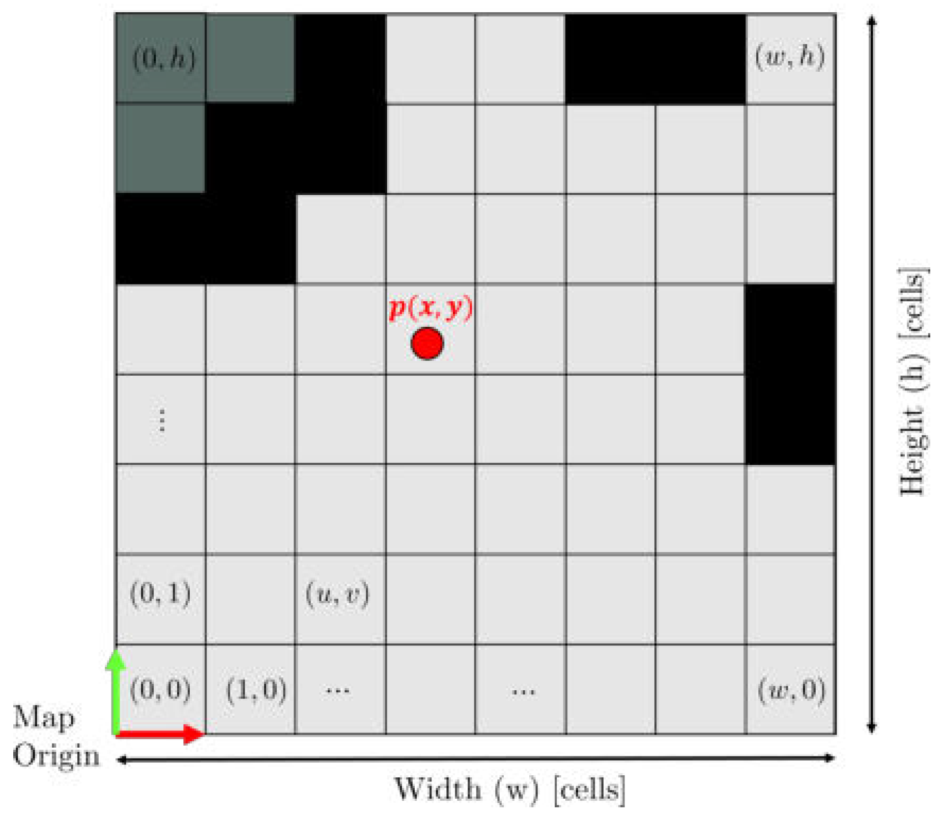
Figure 2.
Ideal case: the laser beam hits an obstacle in . The point identifies the right occupied cell in the map thanks to a correct estimation of the robot position p.
Figure 2.
Ideal case: the laser beam hits an obstacle in . The point identifies the right occupied cell in the map thanks to a correct estimation of the robot position p.
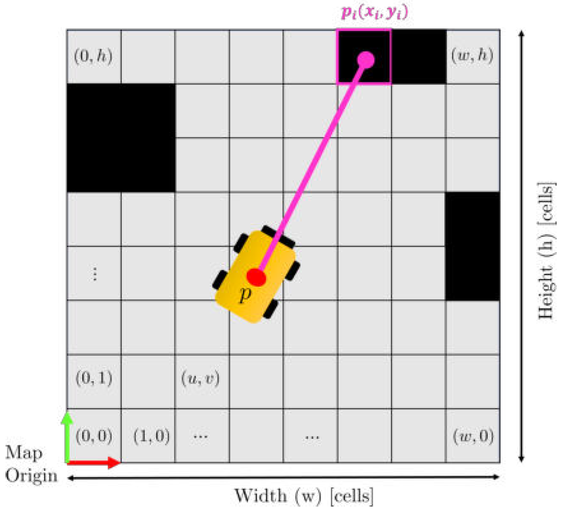
Figure 3.
Real case: due to localisation errors on the robot pose and measurement errors or noises, the laser beams can be prevented to identify the right cell associated with the hit obstacle but another neighbouring cell.
Figure 3.
Real case: due to localisation errors on the robot pose and measurement errors or noises, the laser beams can be prevented to identify the right cell associated with the hit obstacle but another neighbouring cell.
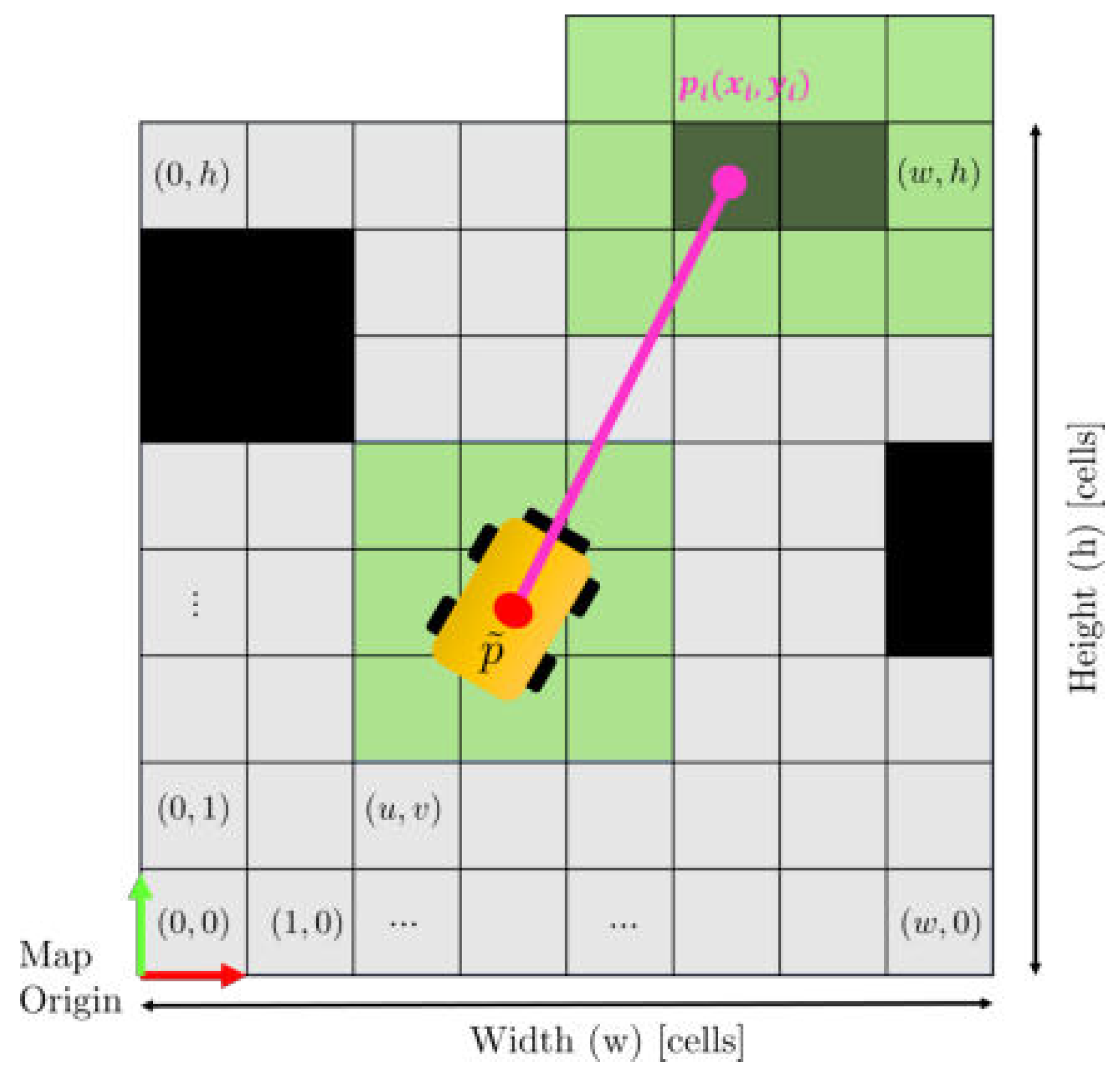
Figure 4.
System Overview: our proposed approach takes as inputs an initial occupancy grid map , the robot pose provided by a localisation algorithm, and the current laser measurements to computes a newly updated map and a new robot pose accordingly to the localisation error.
Figure 4.
System Overview: our proposed approach takes as inputs an initial occupancy grid map , the robot pose provided by a localisation algorithm, and the current laser measurements to computes a newly updated map and a new robot pose accordingly to the localisation error.
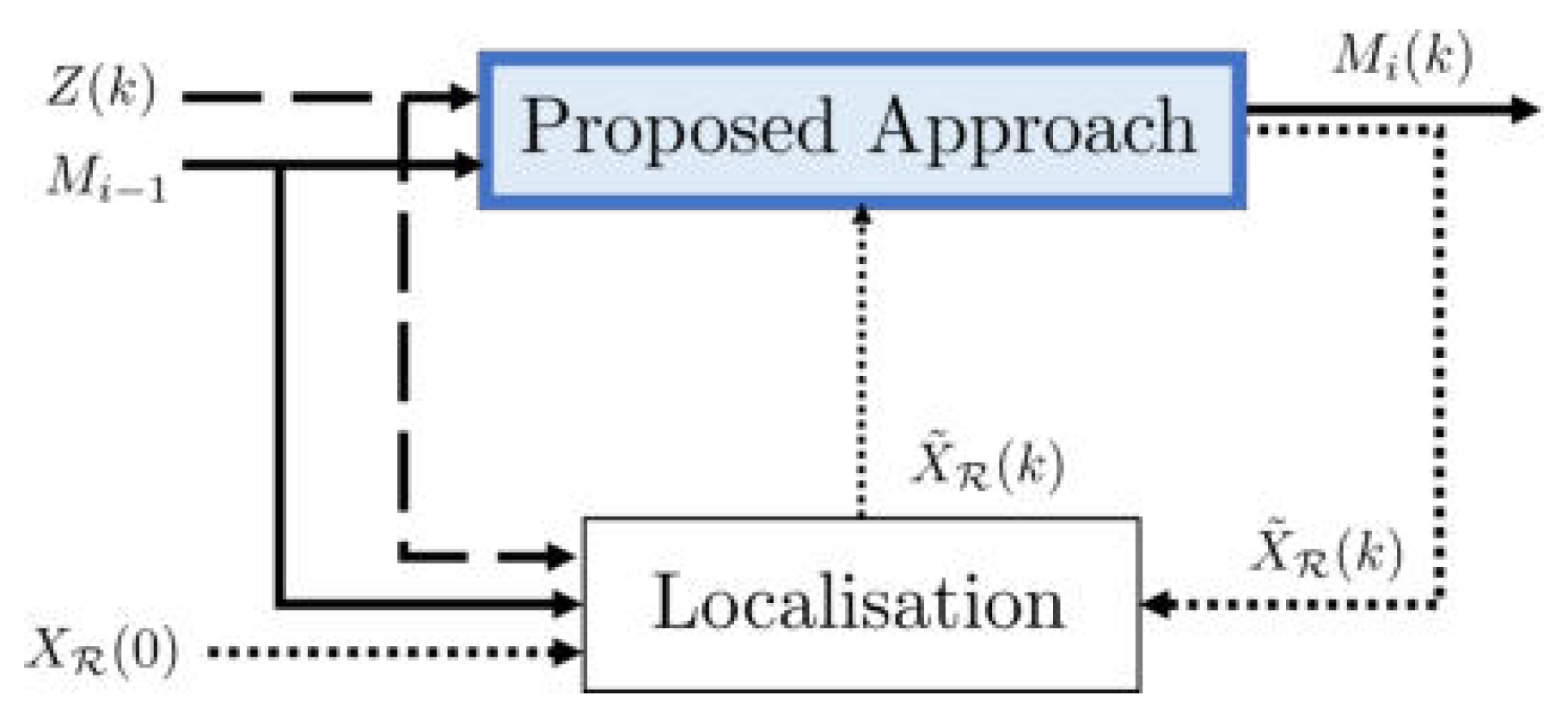
Figure 5.
Proposed Approach Overview: First, the laser measurements are classified with the Beams Classifier as either "detected change measurement" or "non-detected change measurement" based on their discrepancy with respect to the initial map . Then, the detected change measurements are evaluated by the Localisation Check to assess the localisation error. If the error is small enough, the map updating process is activated. Otherwise, the system continues to monitor the localisation error, pausing the map update process until the error goes below a given threshold. On the contrary, if the error continues to increase, the pose updating process is enabled to provide a new based on the last , , and .
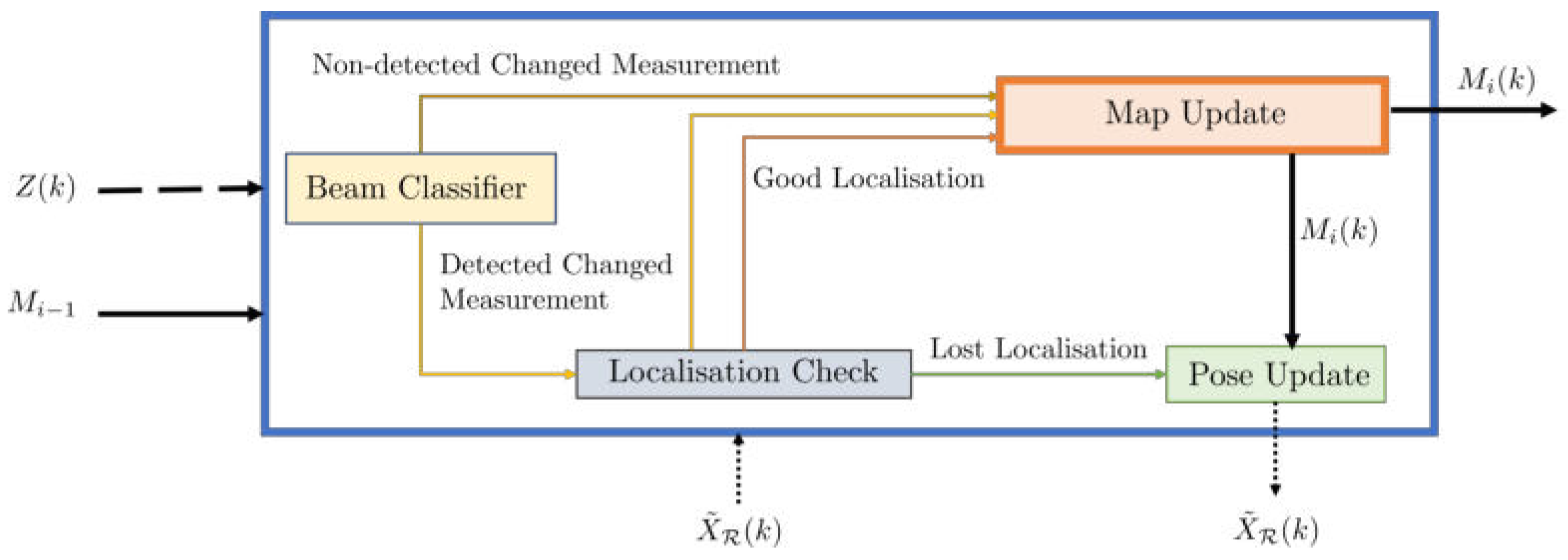
Figure 6.
Overview of Map Updating: Based on the Beams Classifier categorization, the Changed Cells Evaluator and the Unchanged Cells Evaluator fill a rolling buffer of each cell with ”changed” and ”unchanged” flags. Finally, the cells’ status is updated if the number of ”changed” flags in the buffer exceeds a predefined threshold.
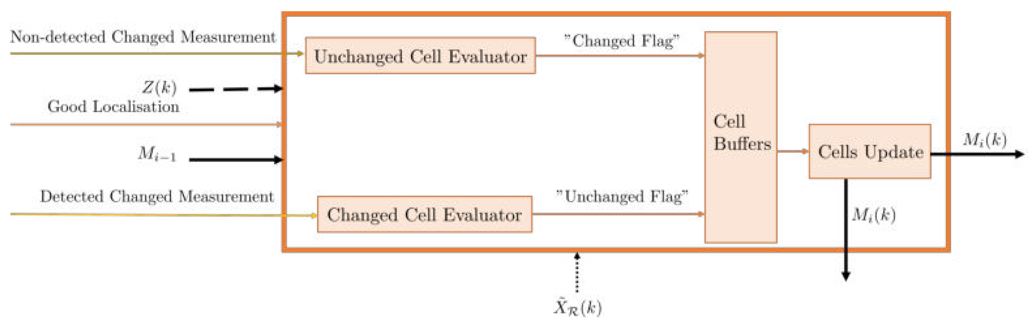
Figure 7.
Example of (in green) with , , and associated to the measured hit point (pink dot). v is chosen so that perturbations , and hence, between and . In this map, the red obstacle has been removed with respect to .
Figure 7.
Example of (in green) with , , and associated to the measured hit point (pink dot). v is chosen so that perturbations , and hence, between and . In this map, the red obstacle has been removed with respect to .
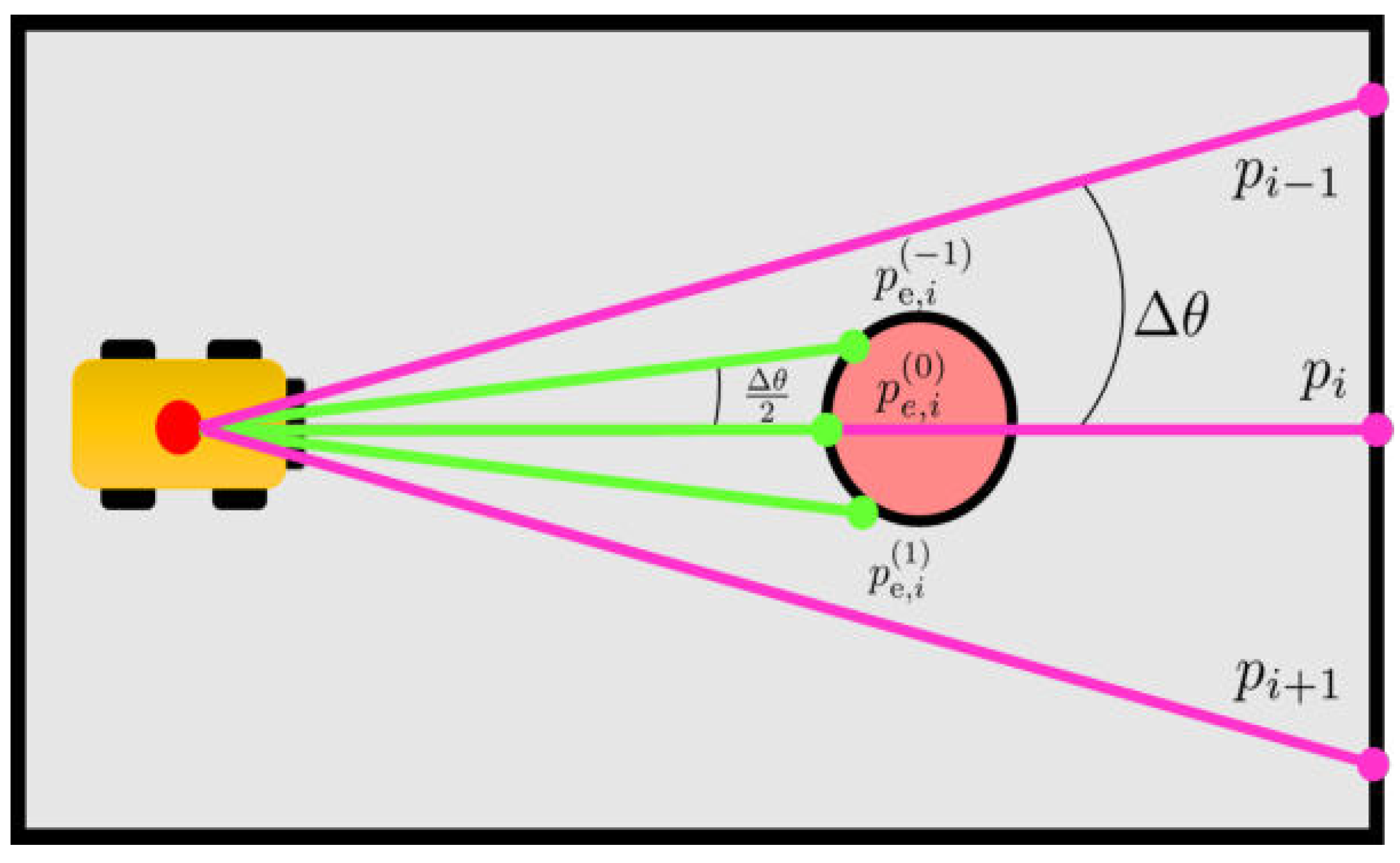
Figure 8.
Example of a measured hit point (pink dot) and differences between single hit point and set of expected measurements (in green) in presence of an obstacle removed from previous map .
Figure 8.
Example of a measured hit point (pink dot) and differences between single hit point and set of expected measurements (in green) in presence of an obstacle removed from previous map .
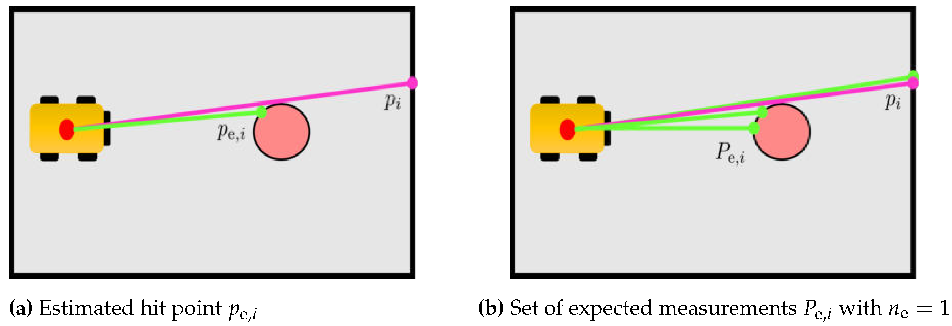
Figure 9.
Examples of ”detected change” measurements caused by an environmental change, such as the addition or removal of obstacles. Pink lines represent laser beams, while pink dots represent the measured hit point. The expected hit points computed on are highlighted in green.
Figure 9.
Examples of ”detected change” measurements caused by an environmental change, such as the addition or removal of obstacles. Pink lines represent laser beams, while pink dots represent the measured hit point. The expected hit points computed on are highlighted in green.
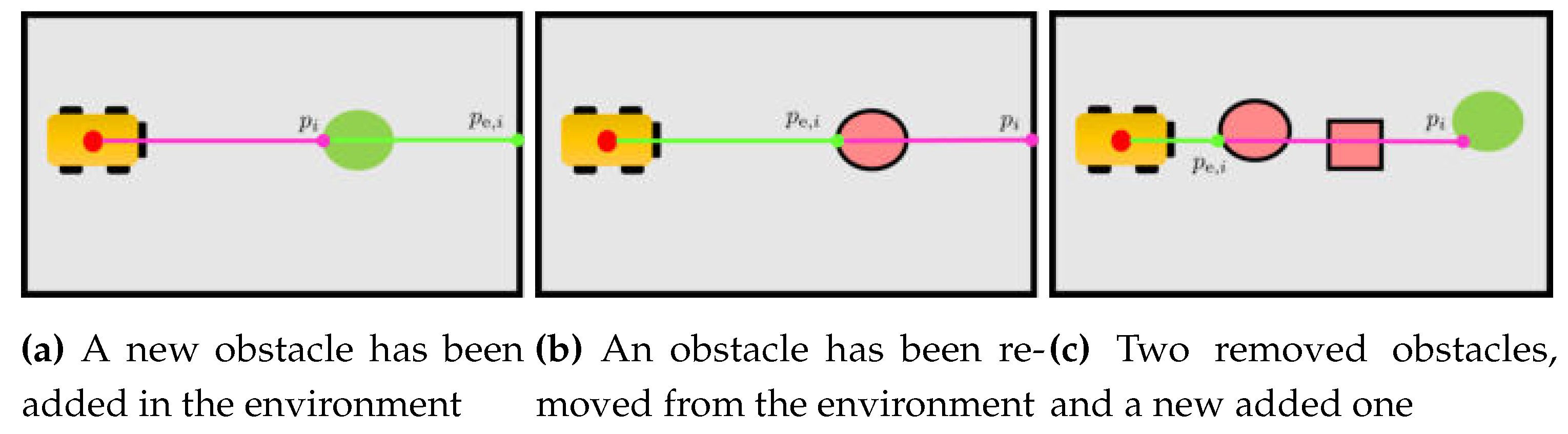
Figure 10.
Example of localisation and noise errors leading to incorrect detection of hit point (in pink), for this reason only cells up to (blue) are examined for change detection.
Figure 10.
Example of localisation and noise errors leading to incorrect detection of hit point (in pink), for this reason only cells up to (blue) are examined for change detection.
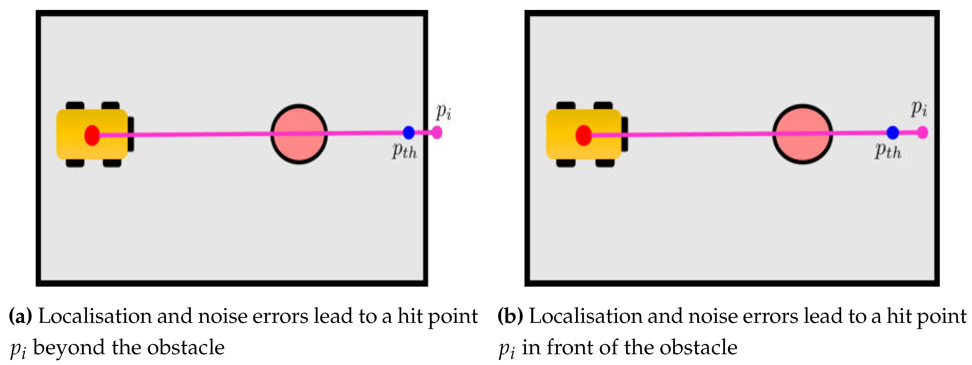
Figure 11.
Ideal case where no localisation error occurs: by checking the current status of the cell associated to the hit point we may distinguish between (a) added obstacle if in , (b) removed obstacle if in
Figure 11.
Ideal case where no localisation error occurs: by checking the current status of the cell associated to the hit point we may distinguish between (a) added obstacle if in , (b) removed obstacle if in
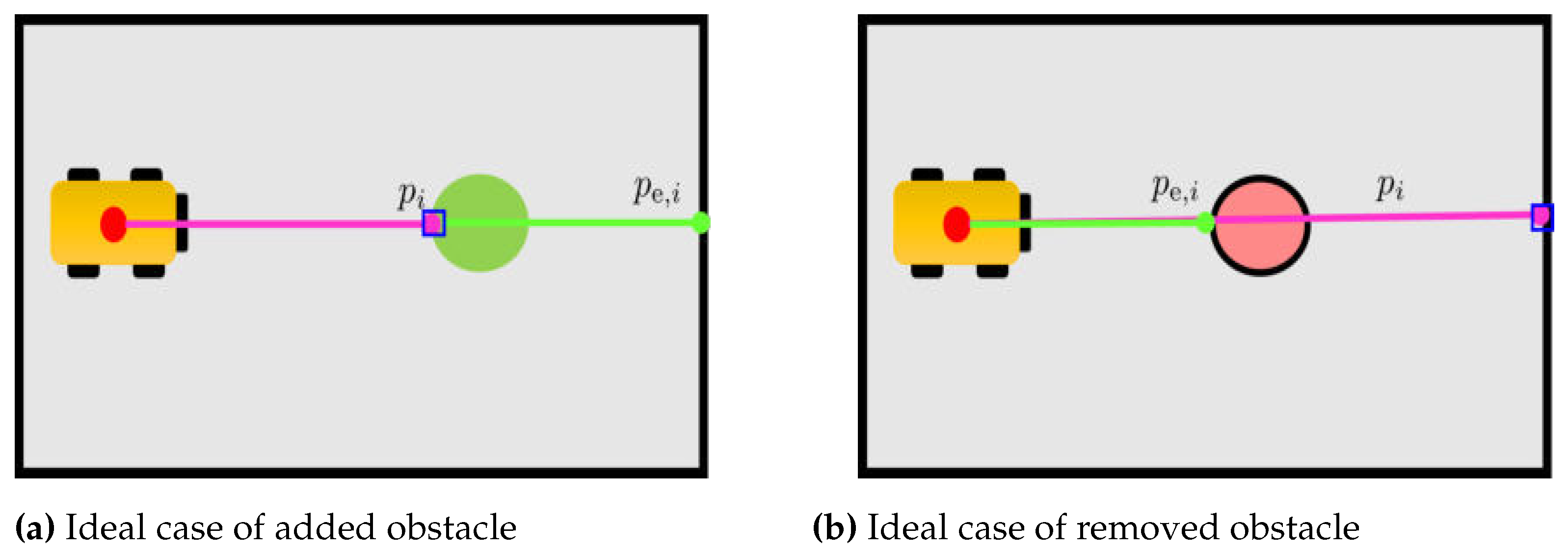
Figure 12.
Case in which localisation error may occur: by checking the current status of the cell associated to the hit point we may not distinguish between (a) added obstacle with in , (b) removed obstacle with in
Figure 12.
Case in which localisation error may occur: by checking the current status of the cell associated to the hit point we may not distinguish between (a) added obstacle with in , (b) removed obstacle with in
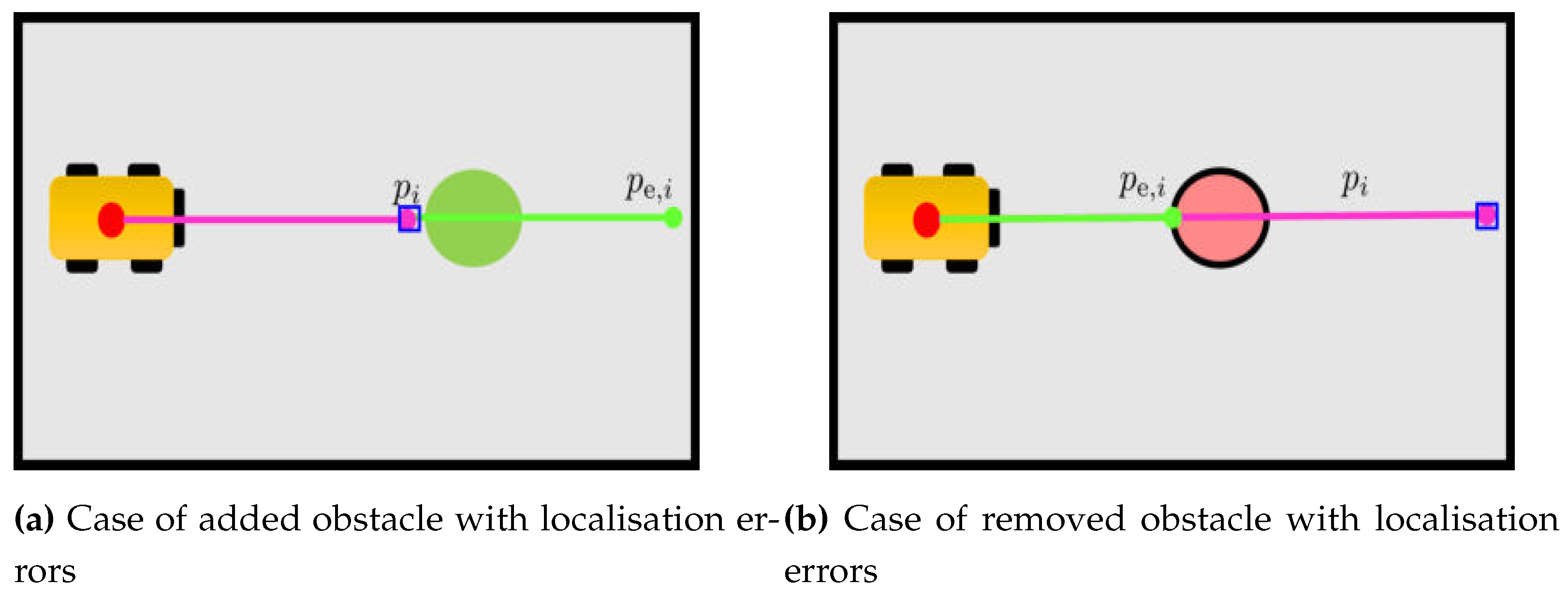
Figure 13.
Considering cells sufficiently close to the system is able to distinguish between an added obstacle case from a removed obstacle one. Case (a), an obstacle has been added, and all cells close to are free in . Case (b), an obstacle has been removed and some cells close to are occupied in .
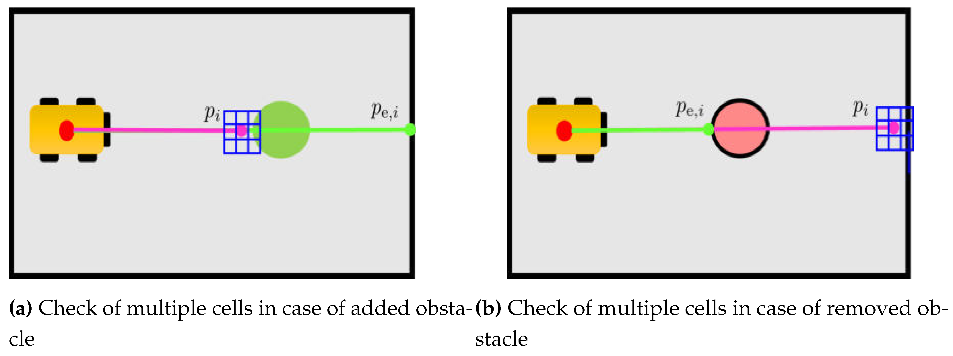
Figure 14.
Last check of free cells to reconstruct obstacle borders
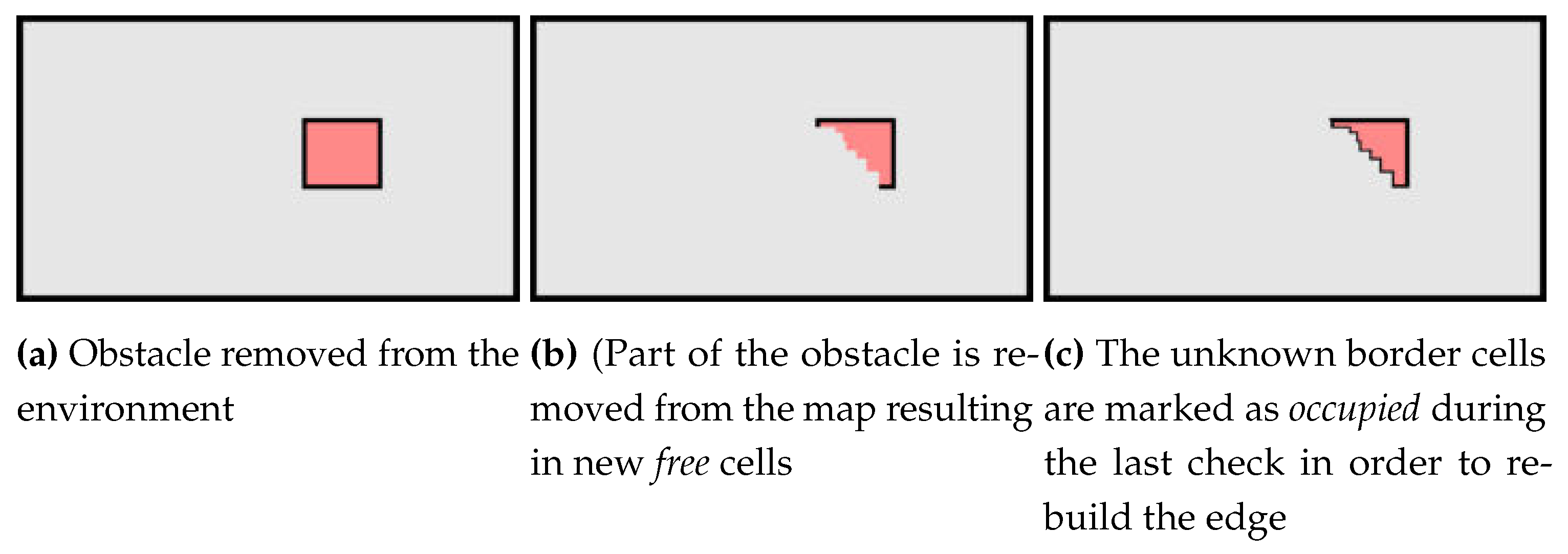
Figure 15.
Scenario for the Localisation Check module testing
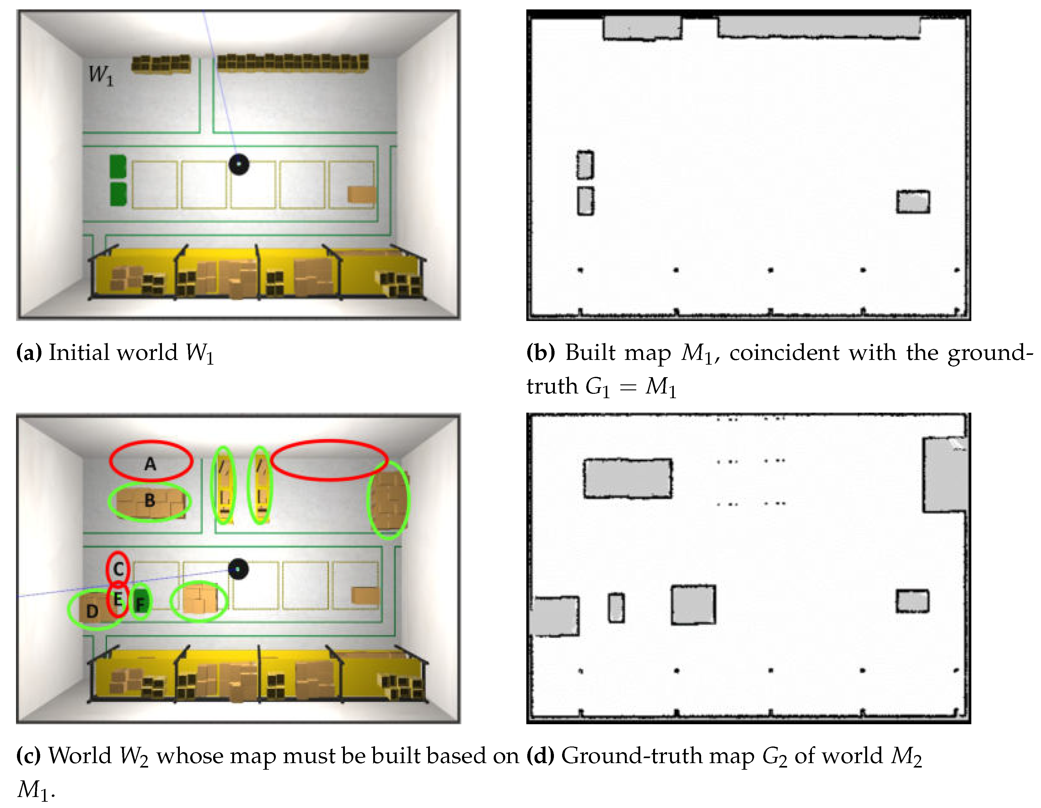
Figure 16.
System evolution at the initial time (a)-(b), after 10 secs (c)-(d), 20 secs (e)-(f) and 60 secs (g)-(h).
Figure 16.
System evolution at the initial time (a)-(b), after 10 secs (c)-(d), 20 secs (e)-(f) and 60 secs (g)-(h).
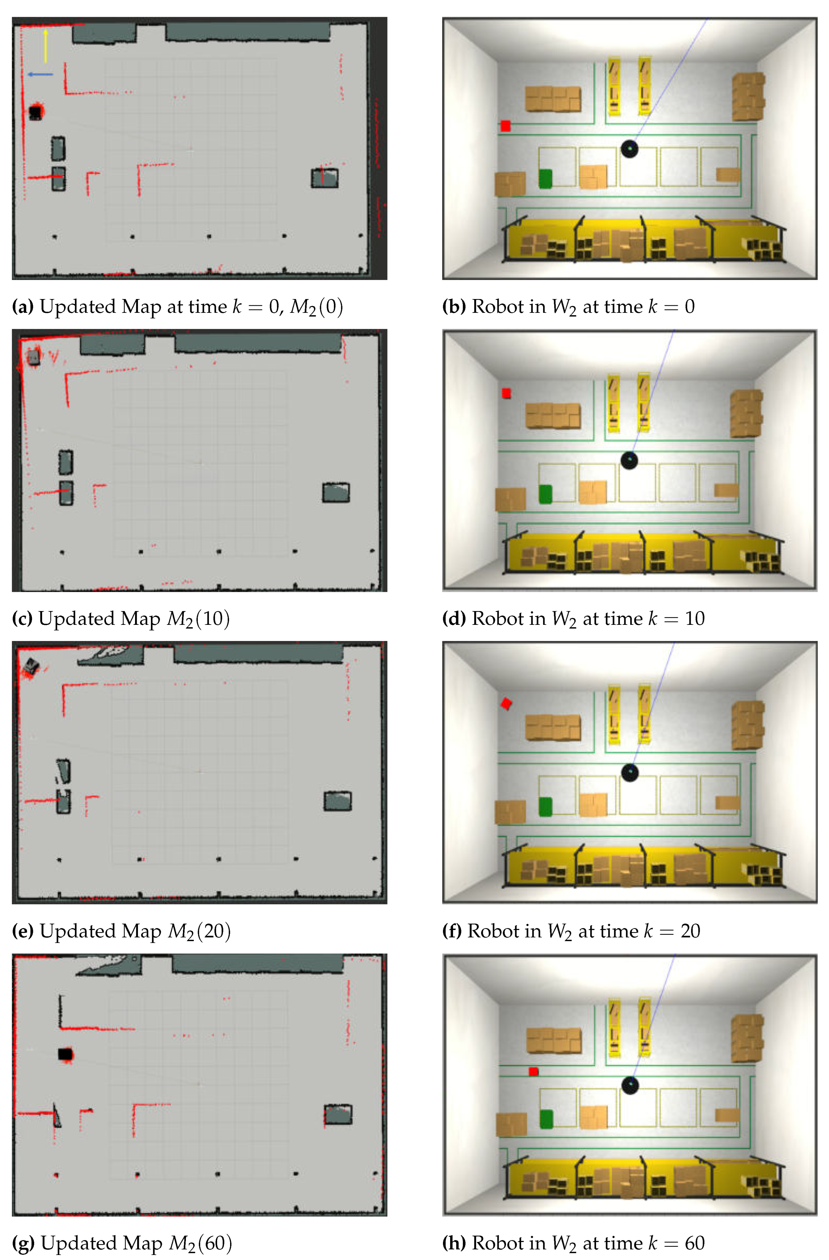
Figure 17.
Scenario for comparison of active Localisation Check module Vs an always active map updating process
Figure 17.
Scenario for comparison of active Localisation Check module Vs an always active map updating process
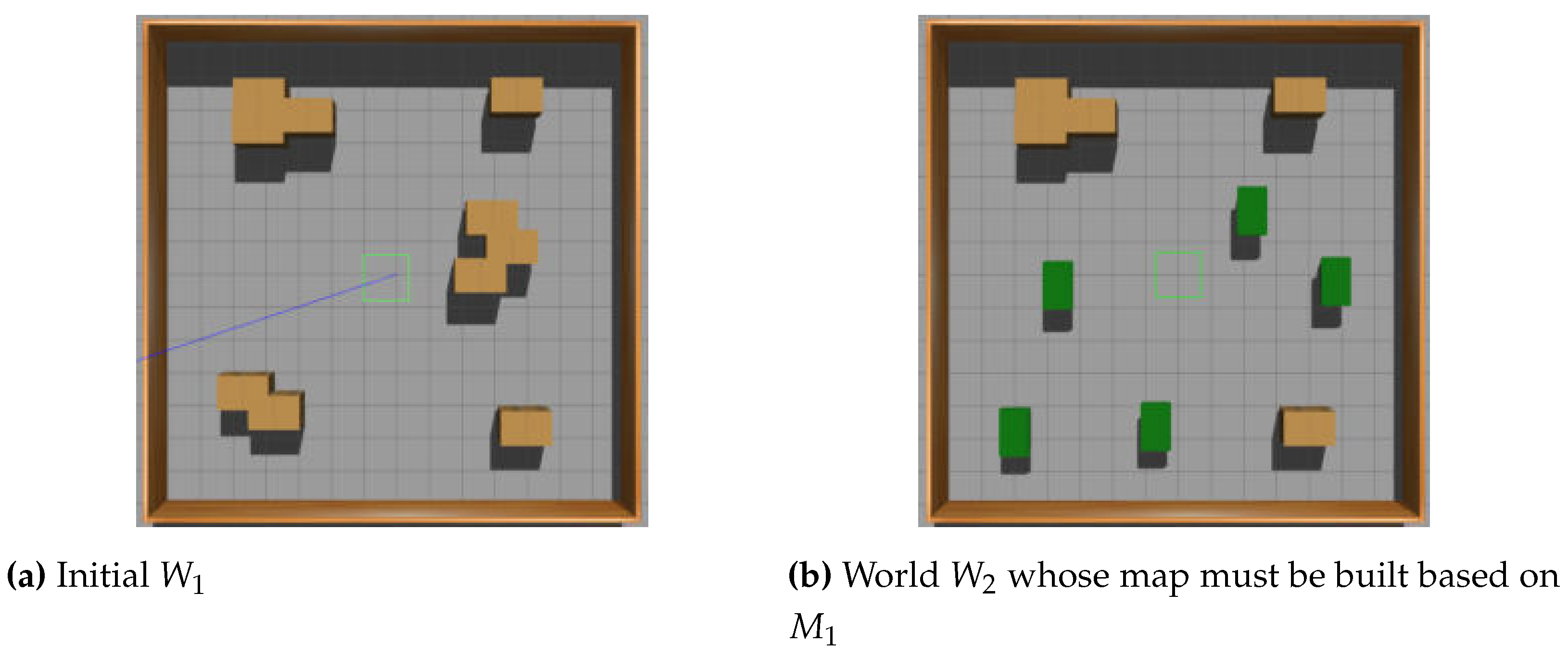
Figure 18.
Initial example configuration
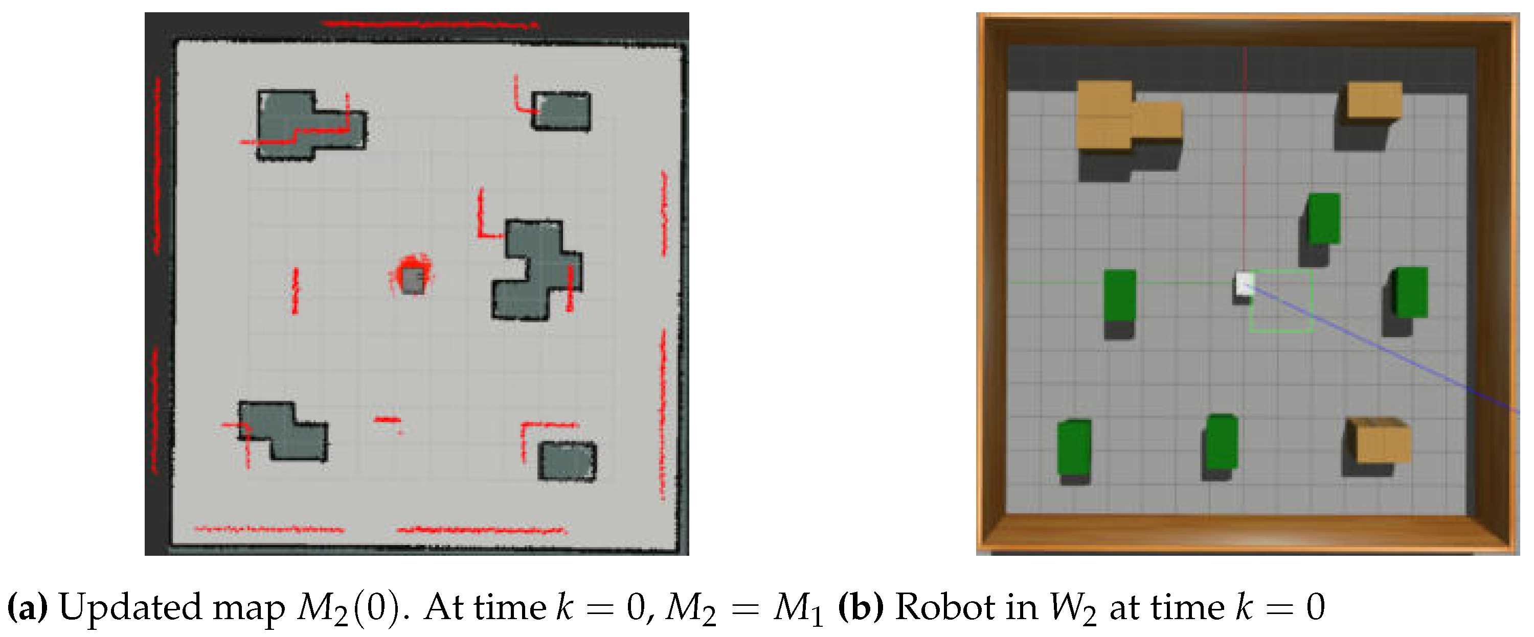
Figure 19.
Updated Mapping Approaches Comparison
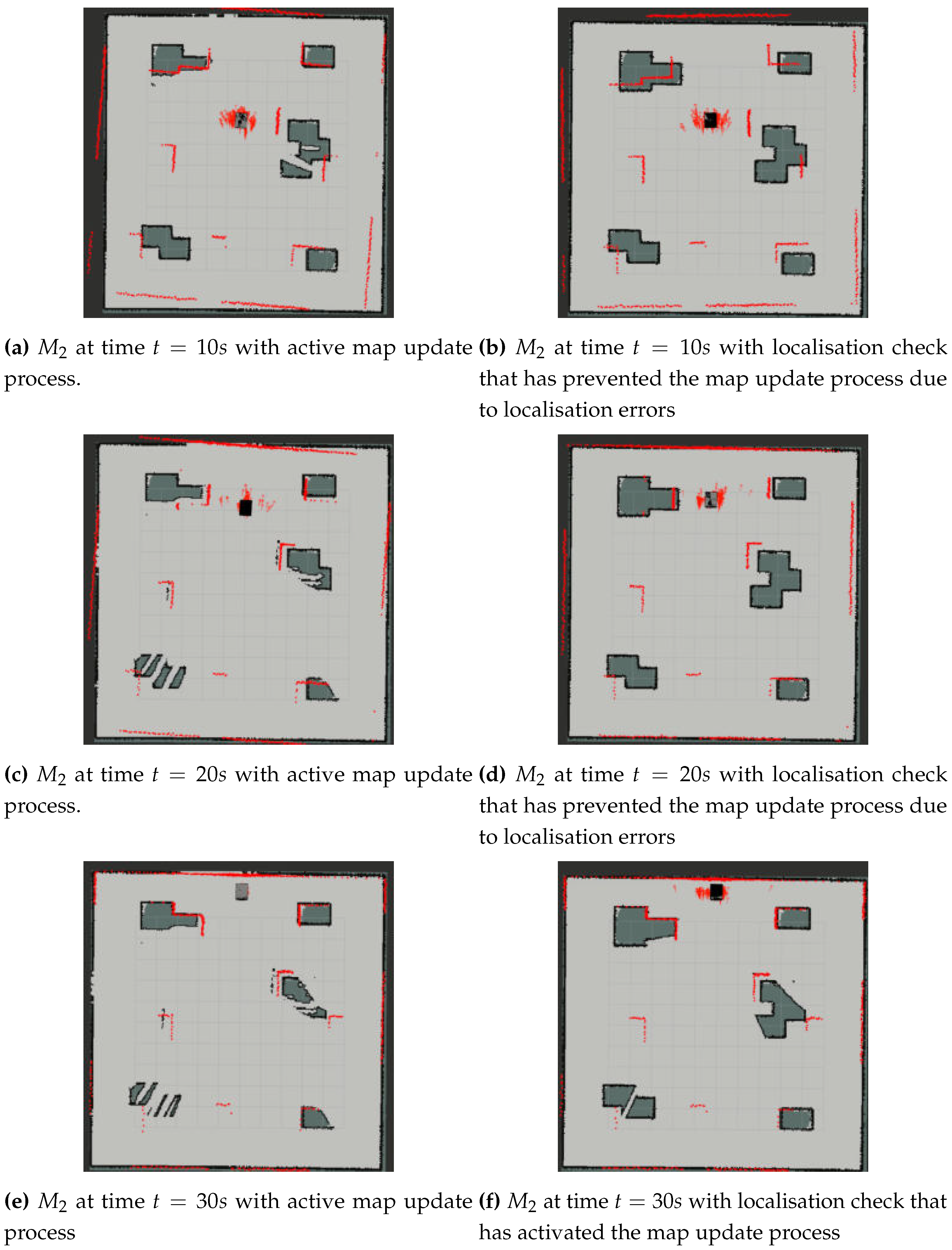
Figure 20.
Maps obtained with the two approaches and the corresponding ground-truth
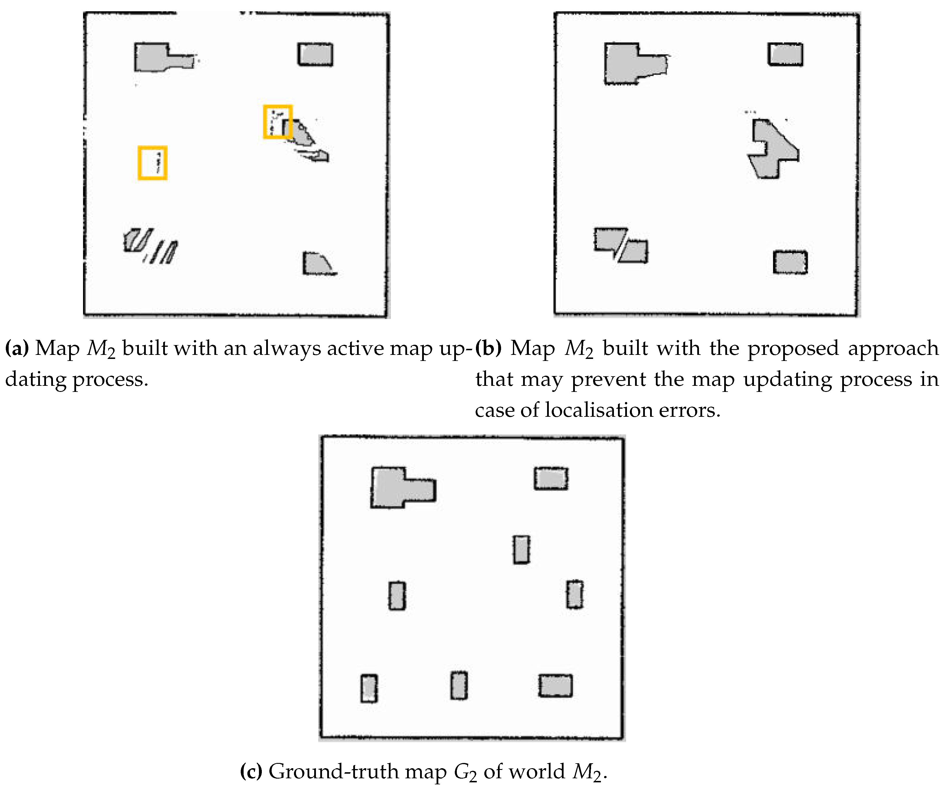
Figure 21.
Warehouse Gazebo environments for worlds 50 and 100.
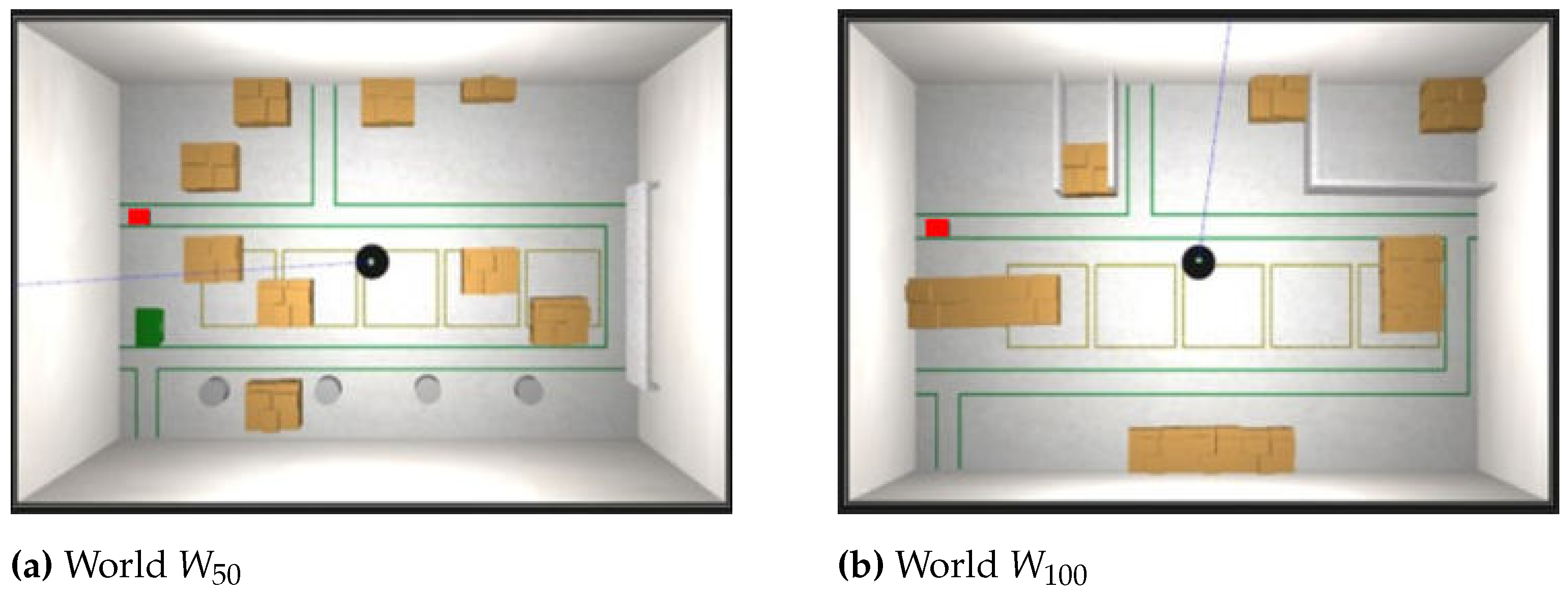
Figure 22.
Autonomous trajectory path (black) in first world (a) and the relative initial map (b)
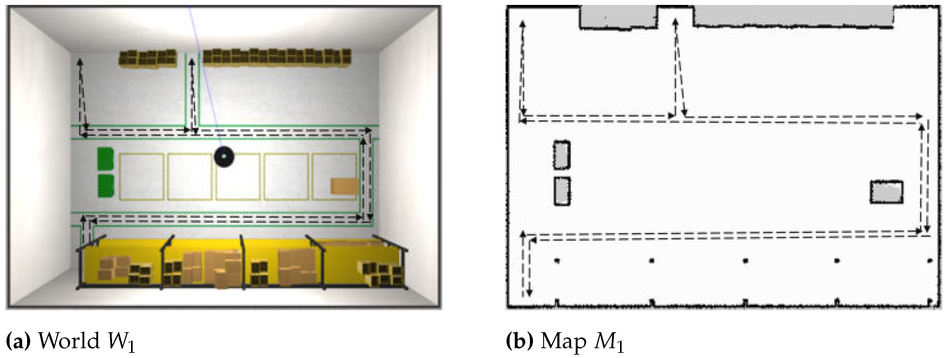
Figure 23.
Map comparisons
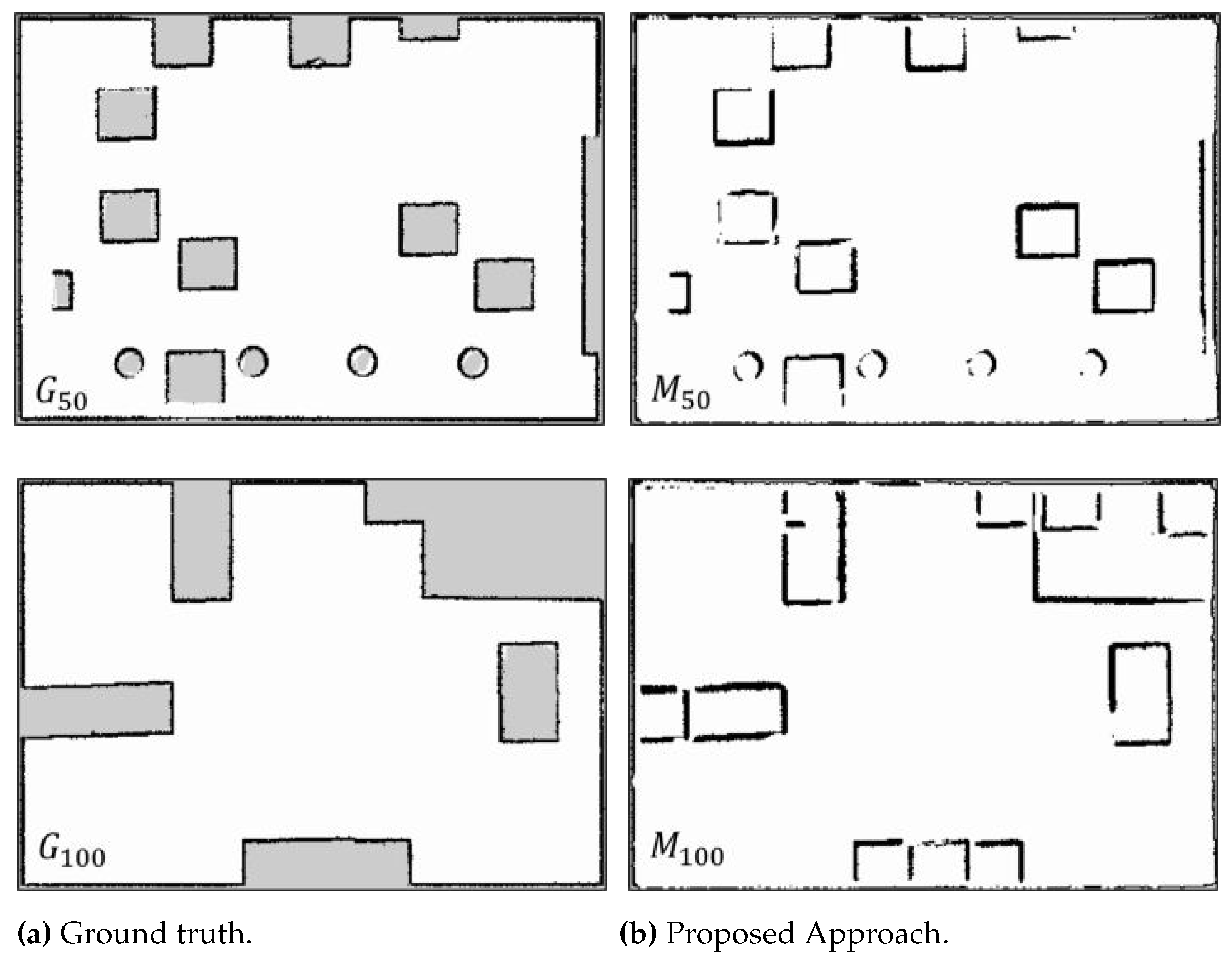
Figure 24.
Quantitative maps evaluation in each simulation scenario.
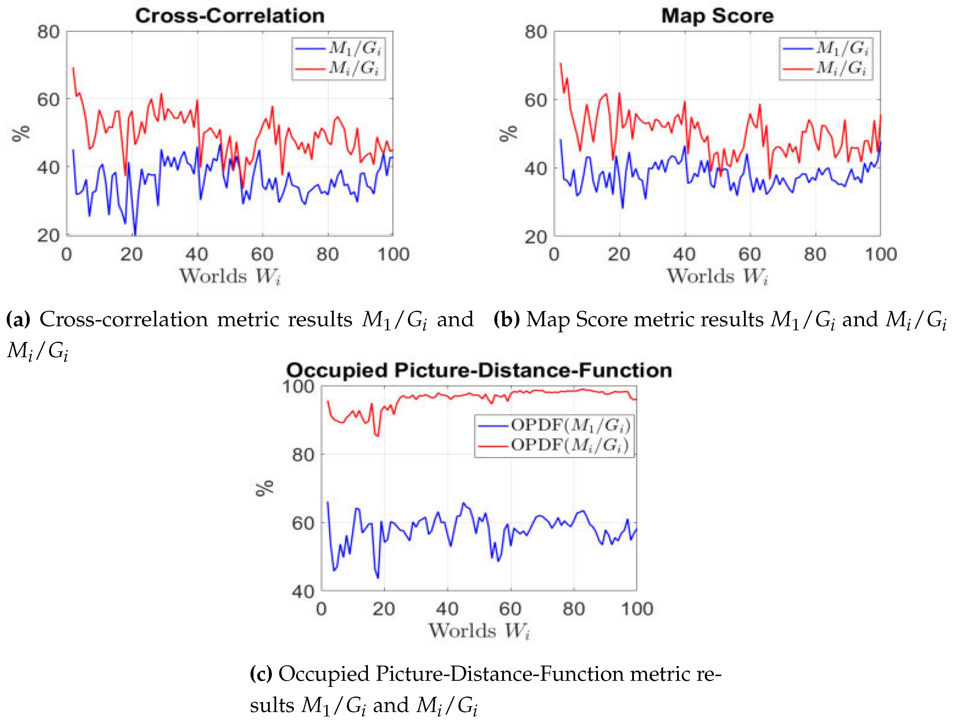
Figure 25.
Localisation Performance: localisation with old map (blue), localisation with last updated map (red).
Figure 25.
Localisation Performance: localisation with old map (blue), localisation with last updated map (red).
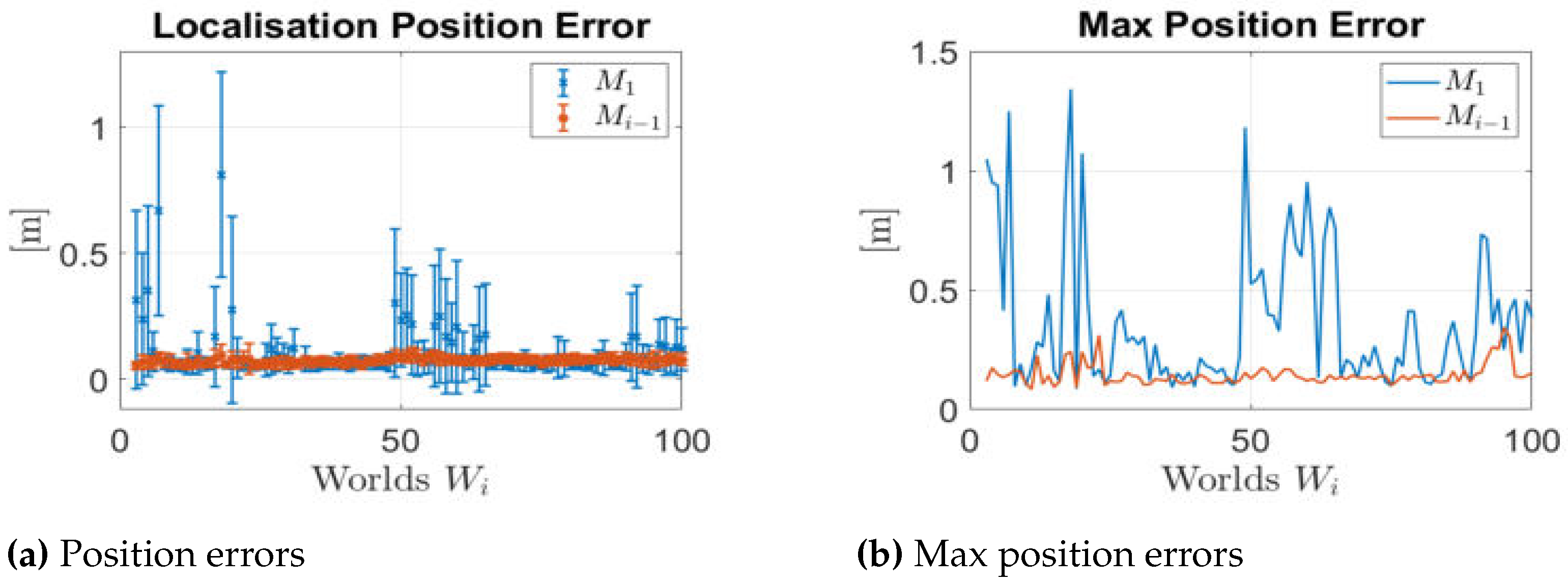
Figure 26.
Estimated Pose Covariance Matrix (P) Results: localisation with old map (blue), localisation with last updated map (red).
Figure 26.
Estimated Pose Covariance Matrix (P) Results: localisation with old map (blue), localisation with last updated map (red).
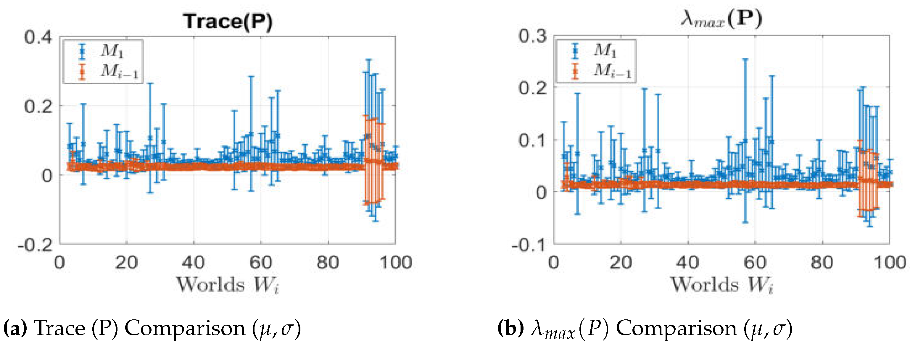
Figure 27.
Resource Consumption
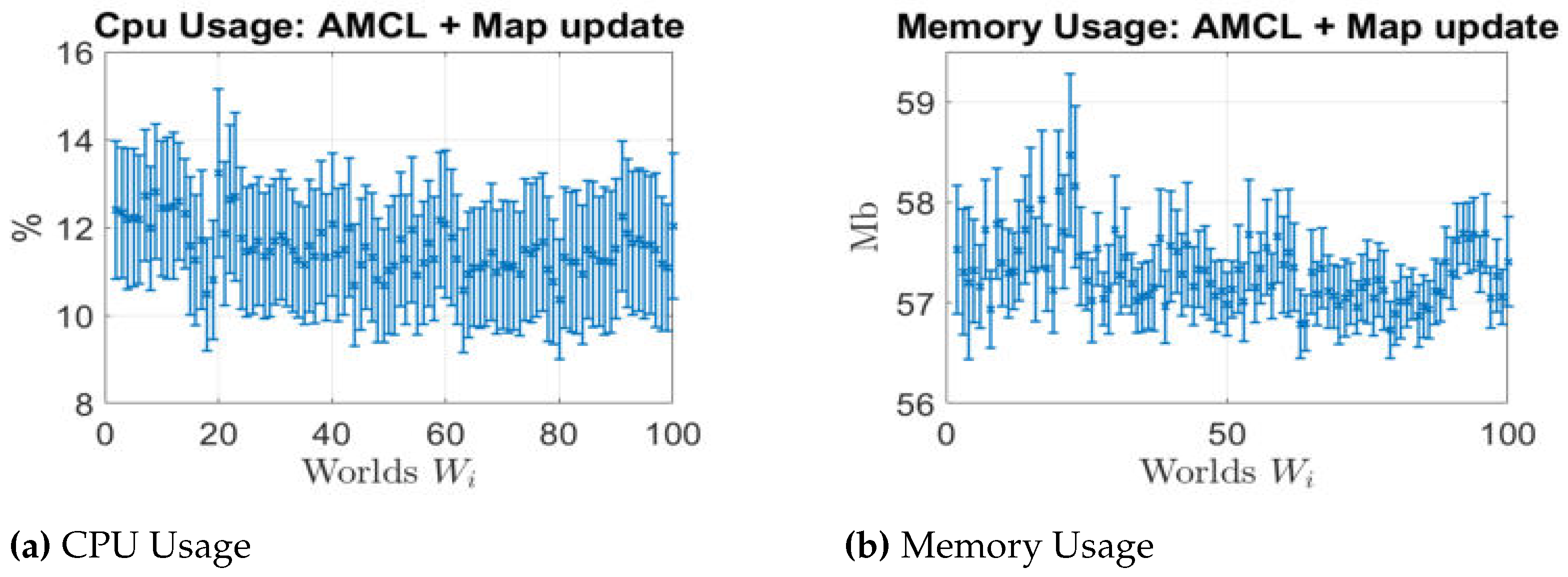
Figure 28.
System evolution at the initial time (a)-(b), after 10 secs (c)-(d) and 20 secs (e)-(f).
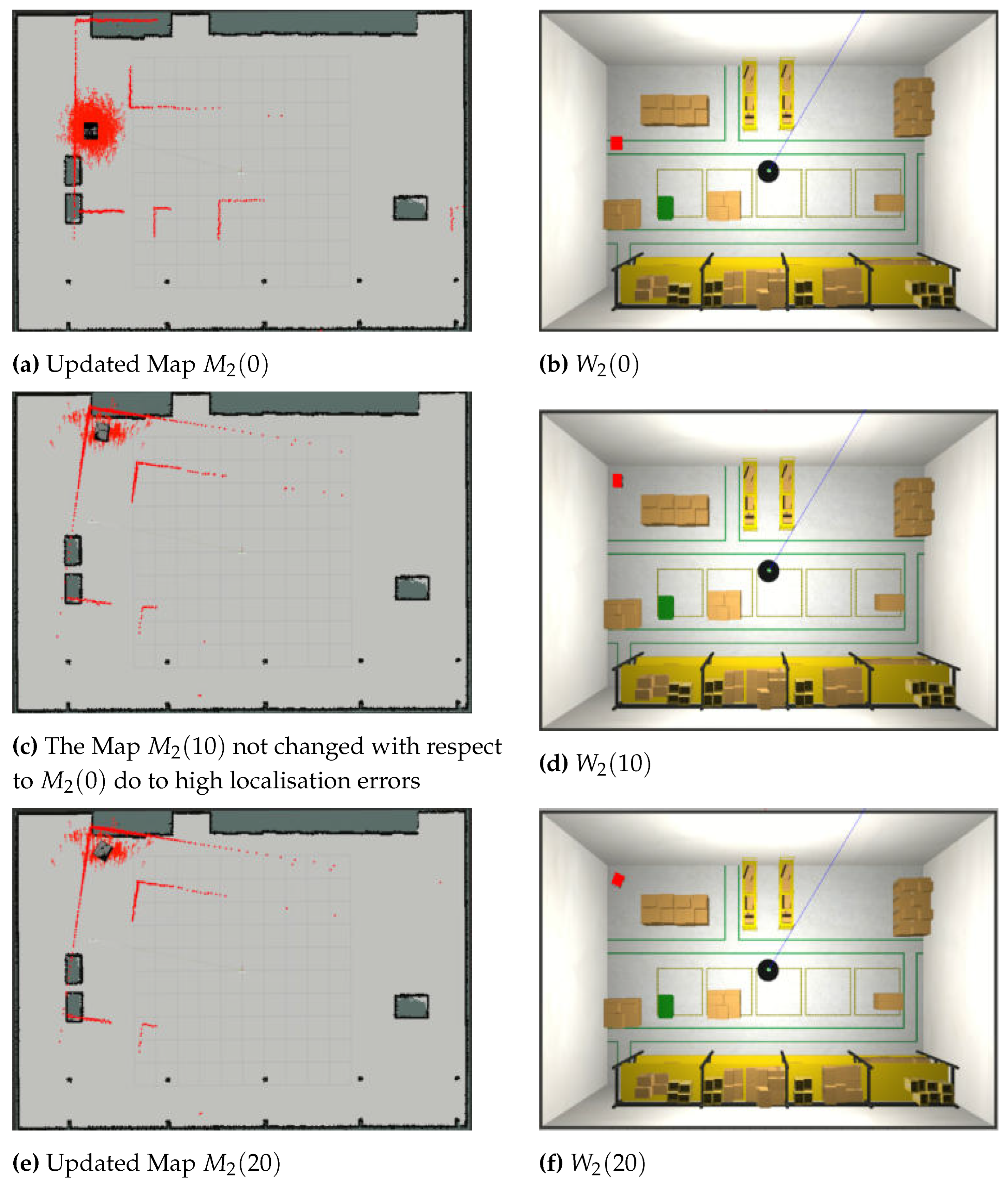
Figure 29.
First case scenario: the map used by the robot to locate itself reflects the current environment, i.e. .
Figure 29.
First case scenario: the map used by the robot to locate itself reflects the current environment, i.e. .
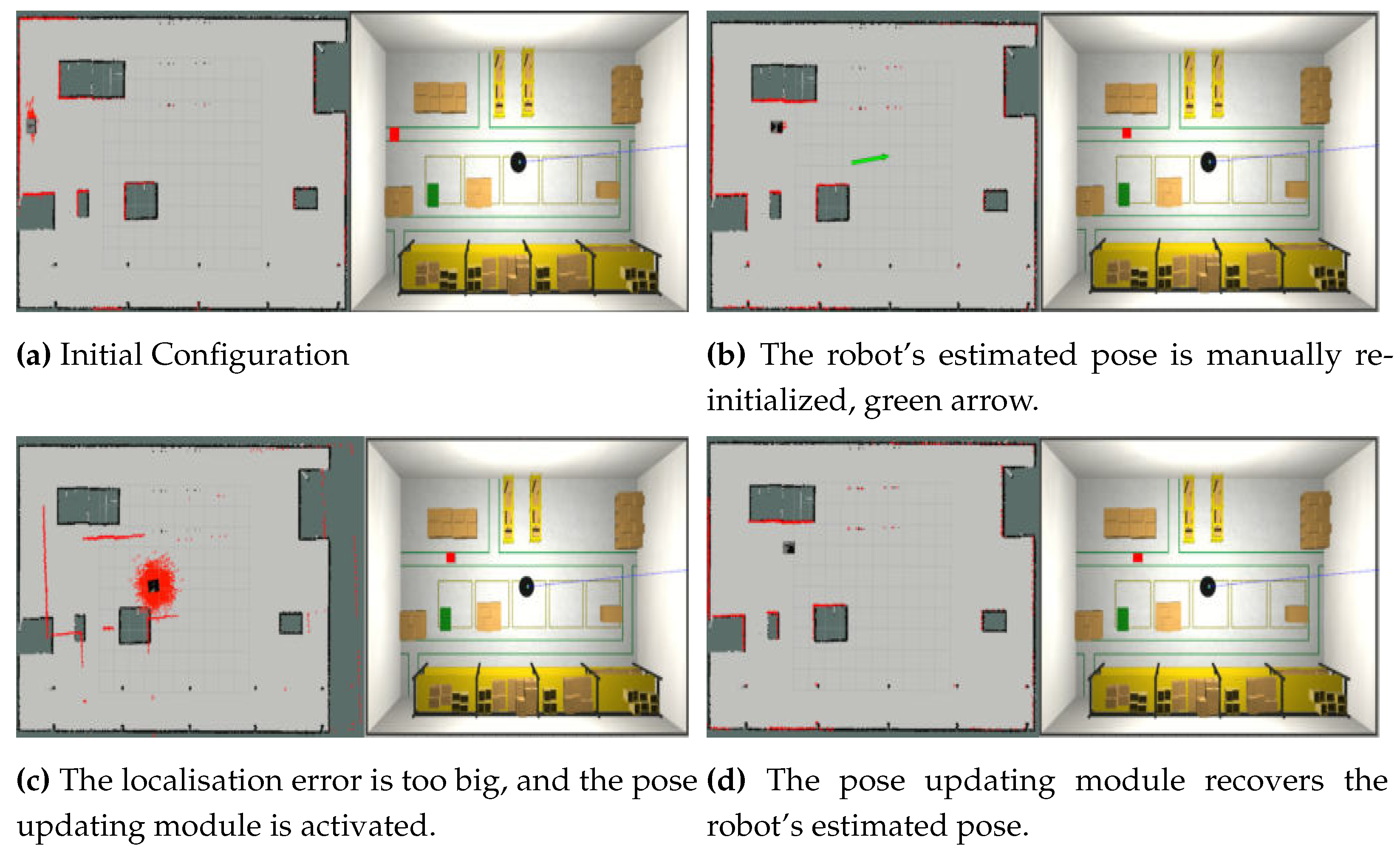
Figure 30.
Second Case Scenario: the map used by the robot to locate itself does not reflect the current environment .
Figure 30.
Second Case Scenario: the map used by the robot to locate itself does not reflect the current environment .
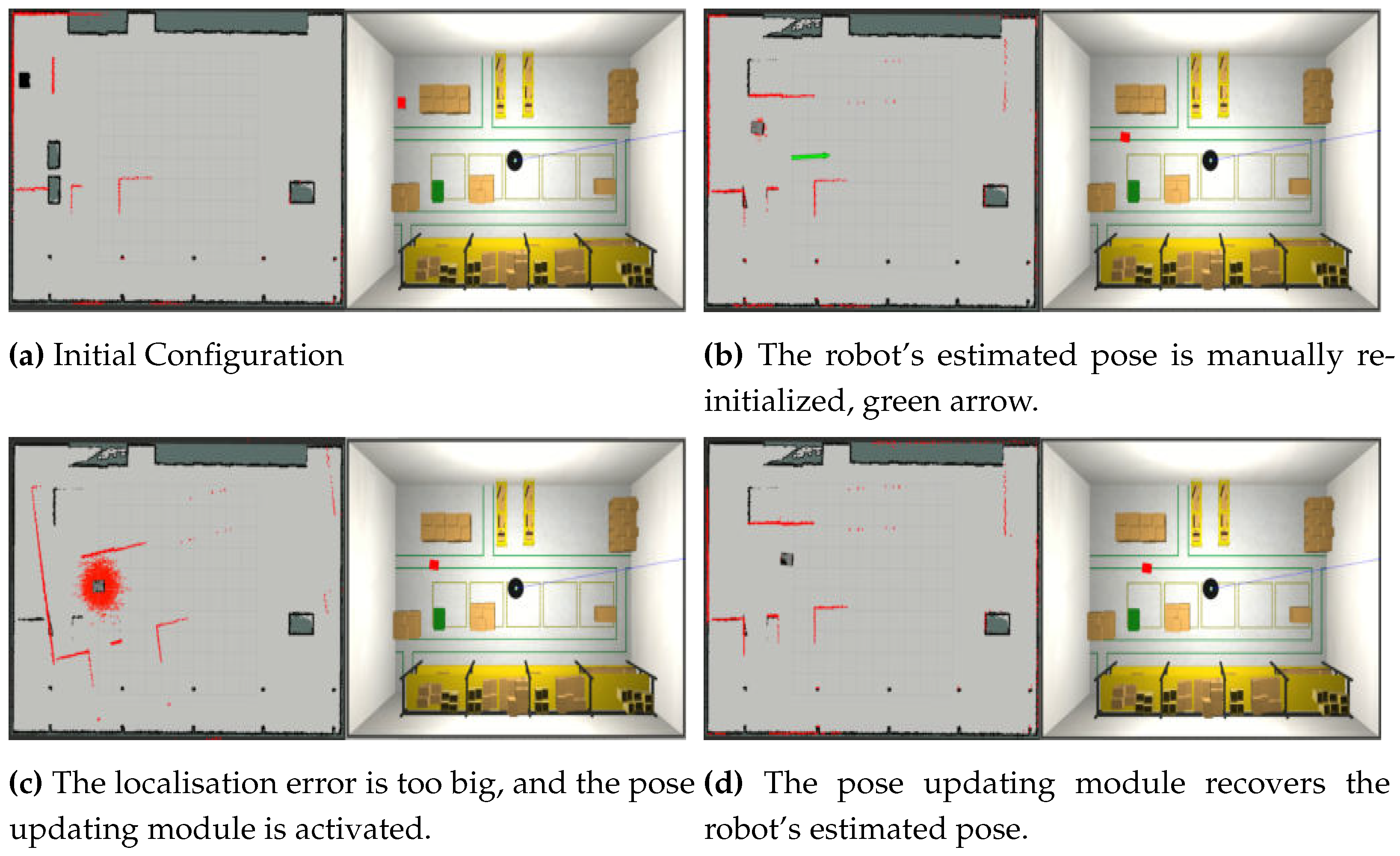
Figure 31.
Lab environment for the experiments
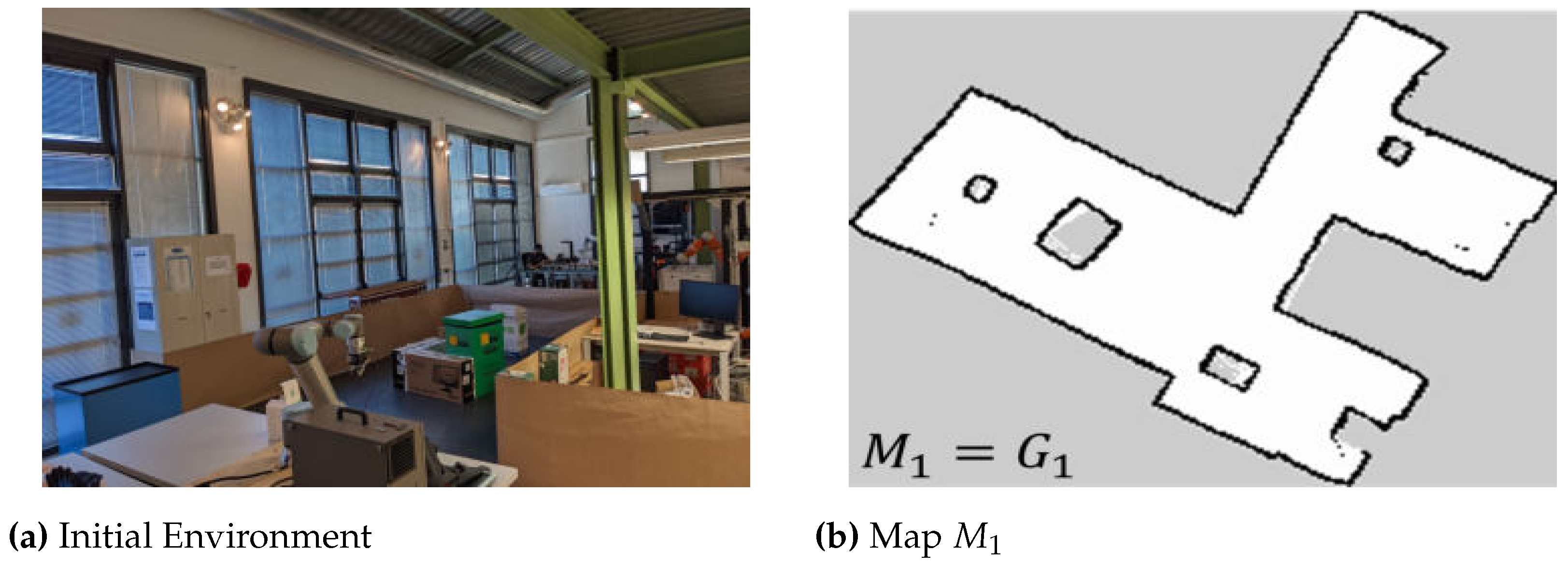
Figure 32.
Map comparisons
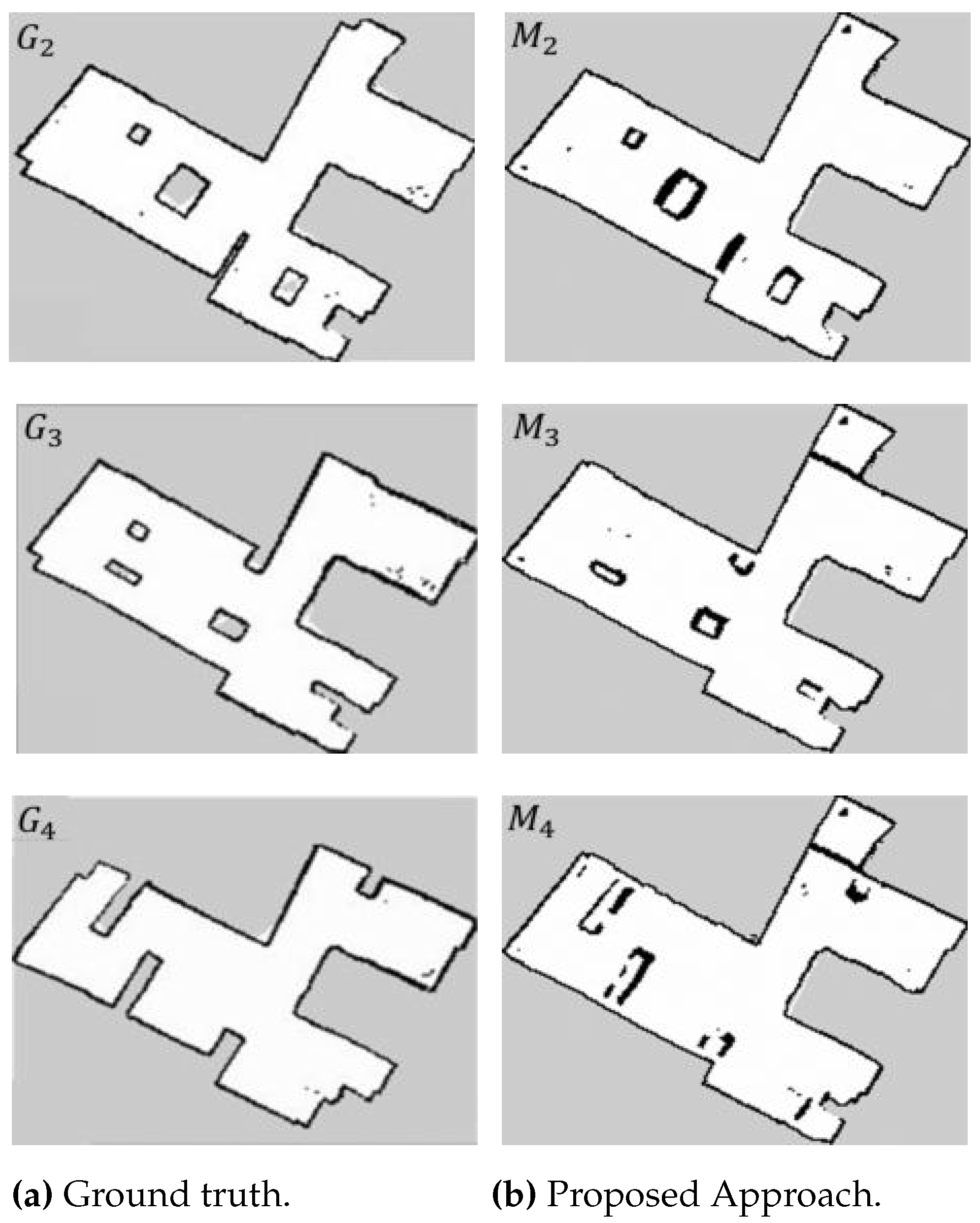
Figure 33.
Estimated Pose Covariance Matrix (P) Results in : localisation with old map (blue), localisation with last updated map (red).
Figure 33.
Estimated Pose Covariance Matrix (P) Results in : localisation with old map (blue), localisation with last updated map (red).
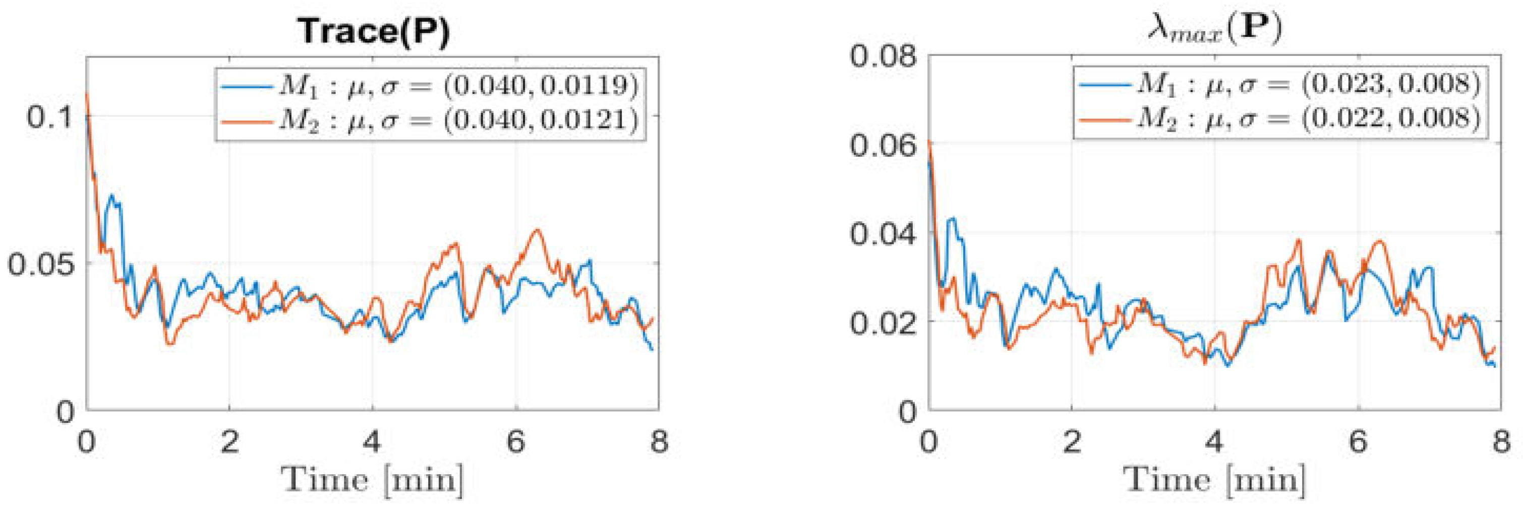
Figure 34.
Estimated Pose Covariance Matrix (P) Results in : localisation with old map (blue), localisation with last updated map (red).
Figure 34.
Estimated Pose Covariance Matrix (P) Results in : localisation with old map (blue), localisation with last updated map (red).
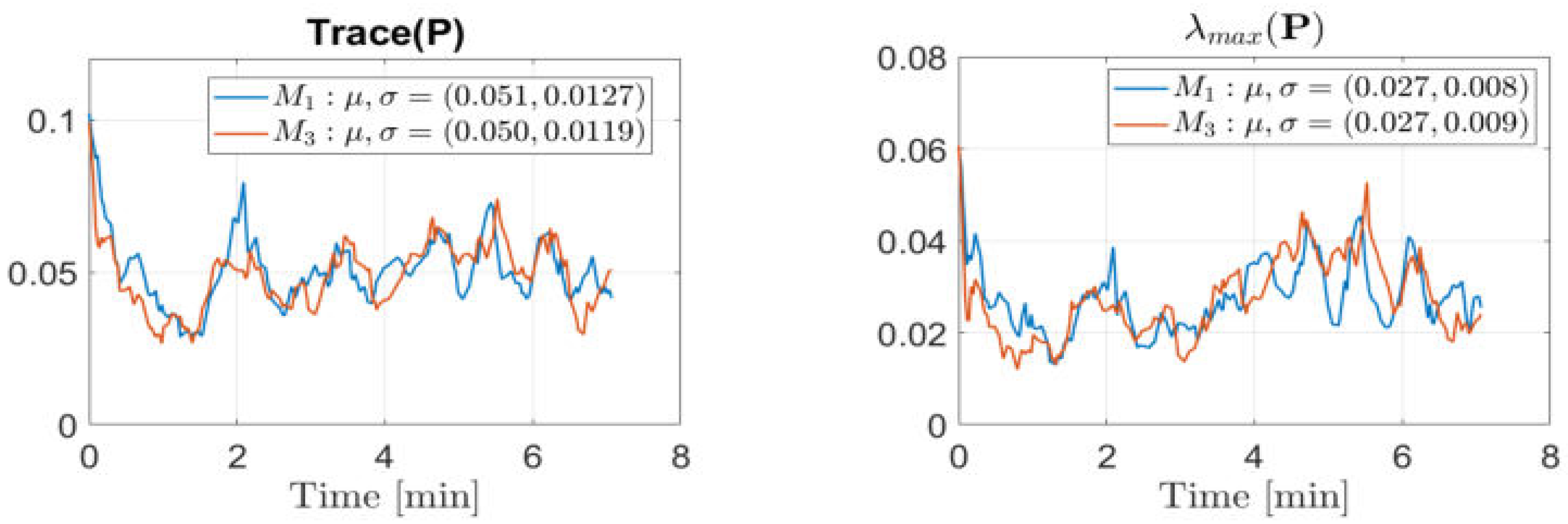
Figure 35.
Resource Consumption
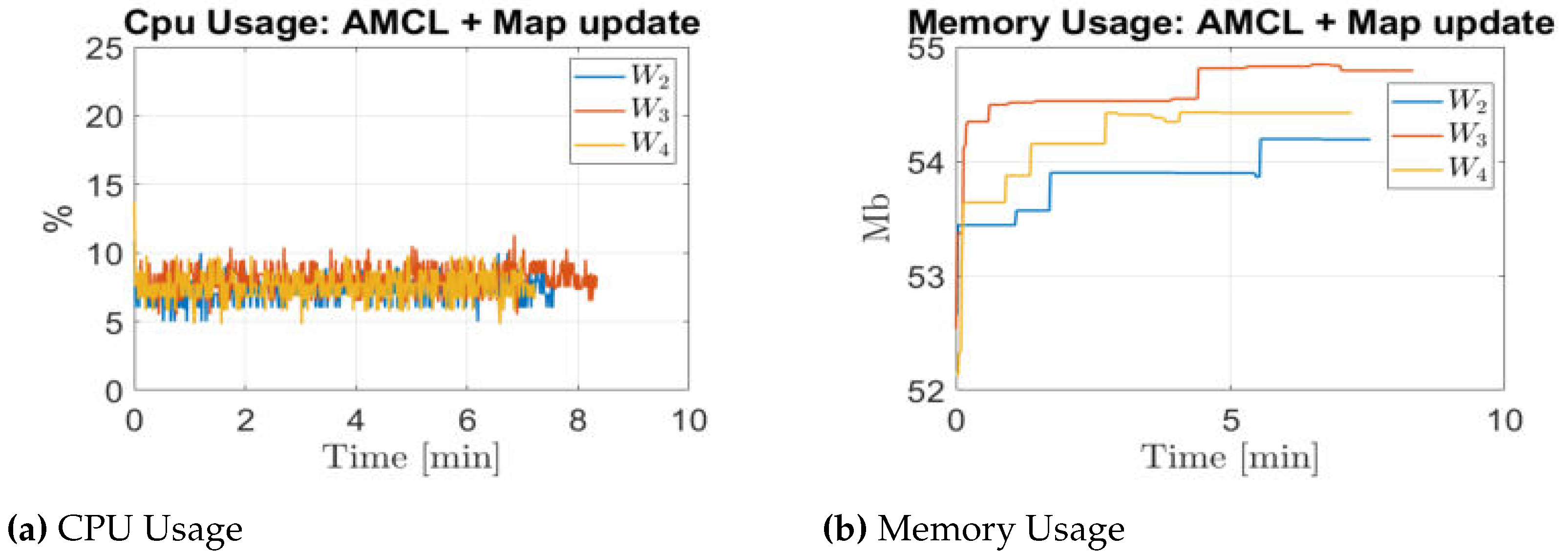

Table 1.
Map Quality Comparison on different metrics
| Old / | New / | |
| CC(%) | 66.86 | 70.03 |
| MS(%) | 55.11 | 61.24 |
| OPDF(%) | 90.40 | 95.87 |
Table 2.
Quantitative maps evaluation.
| CC (%) | 69.69 | 78.95 | 63.77 | 68.80 | 60.87 | 67.14 |
| MS (%) | 54.63 | 74.57 | 51.44 | 72.58 | 50.45 | 70.26 |
| OPDF (%) | 84.61 | 97.25 | 78.92 | 95.37 | 82.18 | 94.33 |
Disclaimer/Publisher’s Note: The statements, opinions and data contained in all publications are solely those of the individual author(s) and contributor(s) and not of MDPI and/or the editor(s). MDPI and/or the editor(s) disclaim responsibility for any injury to people or property resulting from any ideas, methods, instructions or products referred to in the content. |
© 2023 by the authors. Licensee MDPI, Basel, Switzerland. This article is an open access article distributed under the terms and conditions of the Creative Commons Attribution (CC BY) license (https://creativecommons.org/licenses/by/4.0/).
Copyright: This open access article is published under a Creative Commons CC BY 4.0 license, which permit the free download, distribution, and reuse, provided that the author and preprint are cited in any reuse.


