
Submitted:
15 May 2023
Posted:
16 May 2023
You are already at the latest version
Abstract
In the context of Kalman filters, the predicted error covariance matrix $\mathbf{P}_{k+1}$ and measurement noise covariance matrix $\mathbf{R}$ are used to represent the uncertainty of state variables and measurement noise, respectively. However, in real-world situations, these matrices may vary with time due to measurement faults. To address this issue in CubeSat attitude estimation, an adaptive extended Kalman filter has been proposed that can dynamically estimate the predicted error covariance matrix and measurement noise covariance matrix using an expectation-maximization approach. Simulation experiments have shown that this algorithm outperforms existing methods in terms of attitude estimation accuracy, particularly in sunlit and shadowed phases of the orbit, with the same filtering parameters and initial conditions.
Keywords:
Attitude estimation
; expectation maximization
; CubeSat
; extended Kalman filtering
; attitude kinematics
1. Introduction
Cube satellites (CubeSats) are being developed because they are capable of carrying out missions such as earth observation, astronomical physics etc., in place of large satellites [1,2]. Additionally, CubeSats which are predominant in the low earth orbit (LEO) have been considered to be key enablers in global coverage and connectivity [3]. Furthermore, they use commercial off the shelf (COTS) components, which reduces development and production costs. A CubeSat is a standard cubic satellite with a side of 10 cm and a mass of approximately 1 kg. Large CubeSats can be built using several cubic units, for instance, 2, 3 and 6 unit CubeSat. CubeSats have increased access to space by providing low launch cost since they are a carried as secondary payloads in the launch vehicle. Although they are relatively cheap to produce and launch, they have limitations in size, weight, and power (SWaP) and this limits the size and performance of the subsystems [4].
The attitude determination and control system (ADCS) is one of the satellite subsystems, and its key function is centered around steering the spacecraft to its intended orientation. The ADCS can further be divided into two subsystems; attitude determination and attitude control subsystems. The former uses sensors to compute the rotation of a rigid body about its center of mass (attitude) while the latter uses actuators to reorient the rigid body to the desired rotation. The desired orientation could be nadir pointing to allow ground stations to telecommand, or sun pointing to maximize power generation. It is evident in Figure 1 that the attitude determination system (ADS) serves as a reference for control.
The ADS sensors are broadly categorized into reference and inertial sensors. The reference sensors provide directional measurements of the satellite regarding another celestial object in space, for instance, horizon sensors, sun sensors etc. [4]. Inertial sensors are used to determine the rate of attitude change of an object about an inertial frame of reference [5]. These sensors typically include gyroscopes, which are used to measure angular velocity. Since the ADS uses COTS components, the sensors are usually categorized by high noise levels, which affect the systems’ accuracy. The accuracy of CubeSat attitude estimation can also be influenced by the accumulated attitude error over time, which is caused by the drifts of the inertial sensors used.
The attitude determination or estimation algorithms are used to process sensor measurements to compute the attitude. The computed attitude can take several parameterizations, for instance, it may be described using Euler angles, quaternions, axis angle or directional cosine matrix (DCM) [6,7,8]. However, minimal parameterization such as Euler angles, Rodriguez parameters and modified Rodriguez parameters (MRPs)are frequently avoided in filter designs for the global attitude because they can fall victim of singularities, but they are commonly used to define local error attitudes [9]. The most popular attitude parameterization technique is the quaternion since they encounter no singularity problem.
The attitude determination algorithms or single frame methods use measurement vectors provided by reference sensors to calculate an object’s orientation instantaneously. These deterministic algorithms include triaxial attitude determination (TRIAD), Davenport’s q-method, quaternion estimator (QUEST) and single value decomposition (SVD) [10,11]. These deterministic methods have been well-defined in [12], therefore we will not go into detail here. Attitude estimation algorithms make use of vector measurements, inertial measurements and previous attitude information to provide the current optimal attitude estimate. The estimation process can be divided into filtering of sensor measurements and computation of attitude from sensor observations [13]. As stated in [13,14], the filtering process can be accomplished through various methods, such as particle filtering and derivatives of the Kalman filter.
It is common to couple a magnetometer and a sun sensor to measure attitude in small satellites such as CubeSat because each sensor cannot provide 3-axis attitude knowledge independently [15,16,17,18,19]. When one vector is available, the satellite is free to rotate about that vector, thus, at least two vectors are used [15]. When the satellite is in orbit, it passes through regions where the sunlight is blocked by the earth, referred to as eclipse phase. For low earth orbit satellites, they spend about 35 minutes of the orbital time in this phase [20]. During this region, only one vector is available for computing the satellite’s attitude, resulting in high attitude error. The high attitude error affects attitude control accuracy, and this may result in loss of communication during overpasses. It is possible to use additional auxiliary sensors during this phase, but due to the CubeSat’s limited mass and volume, only minimal components are used.
In an attempt to make the attitude estimation process accurate during both sun and eclipse phase, several methods have been employed. Authors in [21] propose the use of magnetic field derivatives as the second vector in the QUEST aided multiplicative EKF architecture to increase the accuracy of attitude estimation during the eclipse phase. Using only magnetometer measurements, the proposed method can estimate rough attitude and angular rate even during eclipse phases; therefore, it can also be used in case of gyroscope failure. In [22], it was found that the SVD-aided EKF outperformed the traditional EKF during the eclipse phase. This improved performance was due to the capability of the SVD-aided EKF to adapt the measurement error covariance matrix () when the ADS lost sensor measurements. During the eclipse phase, when the satellite is in shadow and the reference sensors may not be providing reliable measurements, the SVD-aided EKF utilized an adaptation rule to update the matrix. This adaptation allowed the filter to effectively account for the loss of sensor measurements and adjust the covariance matrix accordingly, leading to improved attitude estimation accuracy. This adaptive behavior of the SVD-aided EKF during the eclipse phase was found to be a significant advantage over the traditional EKF, which did not incorporate such adaptation. As a result, the SVD-aided EKF demonstrated superior performance in terms of attitude estimation accuracy during this challenging phase of the satellite’s orbit, as shown in the research findings by [22]. In contrast, the research revealed that the SVD-aided EKF may exhibit poor performance over a longer period of time (e.g., over 1000 seconds) compared to the traditional EKF, particularly during extended eclipse phases. For instance, in the case of low Earth orbit (LEO) CubeSats, the eclipse phase typically lasts for approximately 35 minutes (2100 seconds), as shown in [20]. As a result, the SVD-aided EKF may not be well-suited for attitude estimation during such prolonged eclipse phases. Another paper [23] proposes a prediction approach for estimating satellite attitude during the eclipse phase, and an adaptive scheme that utilizes the SVD-aided EKF to determine the sun phase. However, the study identified that the accuracy of the prediction algorithm was compromised due to the prolonged duration of the eclipse period.
The SVD-aided EKF was developed as an attempt to enhance the performance of the traditional EKF by incorporating measurement noise covariance matrix adaptation. However, it has been observed that the SVD-aided EKF may face limitations in prolonged eclipse phases. In response, further research has been conducted to develop improved approaches that can make the EKF more adaptable to anomalies such as measurement faults during extended eclipse periods. Researchers in [24], the authors present a technique for computing satellite attitude estimation using an EKF with singular value decomposition (SVD) assistance. The algorithm also incorporates simultaneous adjustments of the process and measurement covariance utilizing data obtained from magnetometers and sun sensors. When the process noise increases or the spacecraft is in eclipse, SVD-aided adaptive EKF performs better than SVD aided EKF. Authors in [25], propose a hierarchical and efficient framework for satellite attitude determination that aims to compensate for observation errors in raw attitude data. It includes a simplified adaptive Kalman filtering module, a neural network-based system error compensation module, and a weighted attitude smoothing module. The performance of the proposed framework, trained with full matrix elements, was found to be comparable to the optimal accuracy when compared with conventional algorithms. Another study in [26] introduces a novel algorithm called adaptive iterated extended Kalman filter (AIEKF) for relative position and attitude estimation, considering model uncertainty in a nonlinear stochastic discrete-time system with unknown disturbance. The AIEKF algorithm employs Gauss-Newton iterative optimization steps for maximum a posteriori (MAP) estimation, and incorporates a switch-mode combination technique to achieve adaptability. The mean-square estimation error (MSE) of the state estimate is derived, and it is proven that the AIEKF outperforms traditional extended Kalman filter (EKF) or iterated extended Kalman filter (IEKF) in terms of MSE.
The structure of the paper is as follows: The attitude estimation and static algorithms are presented in Section 2 in detail. Section 3 provides an introduction to the mathematical models utilized for the presented CubeSat. The proposed filter adaptation method is presented in Section 4. In Section 5, the simulation results of the adaptive EKF algorithm for a hypothetical CubeSat are presented. In Section 6, a brief conclusion is given.
2. Attitude Estimation Algorithms
In this section, we look at the singular value decomposition, extended Kalman filter and their hybrid as they have been proved to be robust algorithms.
2.1. The SVD Algorithm
The SVD algorithm is a deterministic technique for computing the attitude matrix that minimizes Wahba’s problem [11,27]. When more than two sets of measurements are available, Wahba defined a problem aiming to minimize the loss between reference and measured unit vectors. The loss function is
where is the non-negative weight, is a set of reference vectors in the reference frame and is a set of measured vectors in the satellite body frame. An alternative way to simplify the loss function is to use a matrix given as,
where U and V are orthogonal matrices and S is a diagonal matrix with w entries. The optimal attitude matrix is calculated using and matrices, the matrix has a maximized trace and ;
To find the rotation angles of the satellite, a transformation matrix should be found from the (3) first with the determinant of one. To examine the rotation angle error, the error covariance matrix is defined as
where , and When the satellite has only two sensors, that is, the sun and magnetometer sensor, the SVD-method will fail when the satellite is in eclipse because it requires at least two vectors to work properly. This draw back of algebraic methods led to the use of extended Kalman filters for attitude estimation.
2.2. The Extended Kalman Filter
Various estimation techniques have been employed for determining the orientation of satellites. Since Extended-Kalman filters (EKF) are appropriate for nonlinear state equations, they can be used as alternative attitude estimators [28]. Nonlinear discrete time systems can be defined as follows:
where state vector is involved in the system and measurement differential functions denoted by f and h, respectively, y is the expected measurement, w and v is the process and measurement noise with known covariance, respectively. Optimal linear state estimation requires linearizing a nonlinear model about an operating point and applying it to the linearized system. The first order extended Kalman filter uses Taylor series expansion to linearize the system about , other terms are truncated after the first order terms [29]. The EKF consists of two steps: prediction and measurement update, that is,
Prediction step
The prediction step of the recursive extended Kalman filter computes the predicted state vector and predicted error covariance matrix, denoted as and , respectively. is the state transition matrix, which is obtained by computing the Jacobian matrix of the dynamic system nonlinear function f. The state transition can be defined using (15) since it which shows the change of attitude information over time.
Measurement Update
In the measurement update step of the recursive extended Kalman filter, the estimated state vector and error covariance matrix are updated using the Kalman gain and the Jacobian matrix of the differential function in Equation (6), evaluated at . The mathematical formulation of the Kalman gain and are given by
The differential function h can be deduced from the relationship between reference vectors and the satellite measured vectors given by
where is given by (20). The measured vector is the expected measurement given a set of references vector; therefore, it is similar to from (6). From here, the Jacobian matrix is computed based on the resulting vector from (12) to get .
Algorithm 1 provides a summary of the EKF algorithm, in which the variables N and i are utilized to indicate the time window and iteration step, respectively. The inputs of the filter are the initial state , state covariance matrix , sensor measurements , measurement, and process covariance matrices and , respectively. All the other inputs except the sensor measurements are initialized based on assumptions, especially in the absence of covariance data. In the Kalman filter, the state equation consists of kinematics and the accuracy of attitude estimation is determined by how realistic the state model is. Due to the numerous possible disturbances in space, establishing a good state model is difficult. Satellites equipped with 3-axis rate gyros are capable of detecting rotational motion without explicitly modeling disturbances. The rate gyros, however, have biases due to temperature and other factors. As a result, it is generally advisable to estimate the gyro drift rate biases with the attitude parameter.
| Algorithm 1: The extended Kalman filter |
|
Data: inputs:
Result: Optimal state vector
Prediction Step:
1 Compute the Jacobian matrix of to find
2
3
Measurement update
4 Compute the Jacobian matrix of to find
5
6 Update the Kalman gain using (9)
7 Update the predicted state to find the optimal state estimate ,using (10)
8
|
2.3. SVD aided EKF algorithm
The EKF generally performs better than the algebraic methods such as the SVD, however it performs linearization at every stage as shown in Algorithm 1. This computational cost is eliminated by a hybrid algorithm that makes use of both the single frame method and an estimation algorithm such as the SVD aided EKF[24]. The Extended Kalman Filter (EKF) employs the Singular Value Decomposition (SVD) method to obtain a rough estimate of the attitude, such as Euler angles, for state correction. Moreover, the estimation covariance obtained from the SVD is used as the measurement noise covariance matrix in the filter, which inherently makes it adaptive to noise increments in measurements. The SVD acts as a preliminary filter, while the measurement model is linear and the system equations remain nonlinear. In the SVD-aided EKF, the state prediction and measurement model are expressed in discrete time as follows,
where is the linear measurement matrix. The algorithm is summarized in Algorithm 1.
Unlike Algorithm 1, Algorithm 2 makes use of the environmental models’ data because the SVD method uses a set of measured vectors and corresponding vectors in the ECI to compute the rough attitude. The best estimate is computed using the attitude information computed using the SVD method and gyroscope measurements instead of unprocessed vector measurements.
| Algorithm 2: The SVD aided EKF for attitude estimation |
|
Data: inputs:
Result: Optimal state vector
Prediction Step:
1 Similarly as in Algorithm 1.
Measurement update
2 Compute using in (2).
3 Compute the optimal attitude matrix using (3).
4 Compute from (Section 2.1) and use it as .
5 Convert to Euler angles using , and
6 Define the measurement vector using Euler angles and the angular velocity components.
7
8 Update the Kalman gain using (9).
9 Update the predicted state to find the optimal state estimate ,using (10).
10
|
3. System Model
3.1. System Kinematics
The change in attitude of a satellite is modeled using the kinematics equation, which describes rotational motion despite the cause. The kinematic equation of a satellite using quaternions attitude representation is given by
where and r are the components of the angular velocity provided by the gyroscope [30] and is the scalar component of the quaternion. The kinematic equation is useful when defining the state transition matrix in the extended Kalman filter. In this research, quaternions are employed for attitude computation due to their mathematical advantages, such as singularity avoidance and efficient numerical representation. However, for graphical presentation and visualization, Euler angles are used as they are more commonly used in aerospace engineering and provide a more intuitive representation of attitude. This choice allows for a clear and easy-to-understand presentation of the results in a familiar format. The computed quaternion is converted to Euler angles using;
3.2. Environment Models
3.2.1. International Geomagnetic Reference Field (IGRF)
The IGRF denotes the main geomagnetic field generated by internal sources, primarily inside the core of the earth [31]. The absence of electric currents on the surface allows for the computation of the Earth’s geomagnetic field as the negative gradient of a scalar potential, such that the magnetic field can be expressed as . The potential function is represented by a finite series expansion in terms of Gauss coefficients, and [32]:
Here, is the radial distance from the Earth’s center, geocentric co-latitude, longitude and time respectively. The variable a is the Earth’s radius. More information of the spherical harmonic coefficients can be found in [31]. The latest version in the series, IGRF-13, extends up to thirteen harmonic degrees.
3.2.2. PSA Sun Position Algorithm
The paper utilizes the PSA algorithm to calculate the solar vector in the inertial frame due to its small computational footprint and high accuracy. It has been established that when applied over a period ranging from 2020 to 2050, the maximum error in angular deviation from the actual solar vector is only 35 arc-sec, with the algorithm maintaining its computational structure and simplicity [33]. The PSA algorithm’s inputs consist of the location’s latitude and longitude, along with the time specified in universal time (UT1), encompassing year, month, day, hours, minutes, and seconds. The sun vector is given by
where and is the zenith and azimuth angle. More information on how these angles are obtained can be found in [33].
3.3. Measurement Model
In this model, we assume that only zero-mean Gaussian white noise can corrupt the sensor measurements. The measurement model for the vector observations can be given as
where is the sun and magnetic field vector observations in the body frame, can either be or modelled in the reference frame, is the Gaussian white noise and is given by (20).
For gyroscopes, the inherent sensor bias introduces errors throughout the attitude determination process; therefore, these errors are also included in the state vector estimate. The gyroscope mathematical model presented in this paper is
where gyroscope noise and bias of a satellite are represented by and , respectively, while the true angular velocity of the satellite relative to the inertial frame is denoted by .
3.4. Coordinate Systems
Several reference frames are used to describe the satellite’s attitude. This paper employs three reference frames, each of which is defined by its fixed element or direction, as well as by the location of its center or origin, that is, satellite body coordinate frame, orbit referenced coordinate frame and Earth Centered Inertial (ECI) coordinate frame. These coordinate frames have been well explained in [14].
4. Adaptive EKF
During extended eclipse phases, it was noted that the traditional Extended Kalman Filter (EKF) exhibited superior performance compared to other methods like the Singular Value Decomposition (SVD)-aided EKF. However, if the accuracy of the process and measurement noise covariance matrices is compromised, the EKF may produce substantial estimation errors, despite outperforming other algorithms in prolonged eclipses. As a result, there is a great need for developing an adaptive EKF that is compatible with inaccurate covariance matrices. Firstly, we discuss how each covariance matrix affects the performance of the extended Kalman filter (EKF). The process noise covariance matrix can cause inaccurate prediction of the error covariance matrix in (8) which directly affects the computation of the Kalman gain as shown in (9). Finally, the optimal estimate and the estimated error covariance matrix are derived from the incorrect and as seen in (10) and (11), respectively. Additionally, it is clear that an imprecise measurement noise covariance matrix can lead to an imprecise Kalman gain, resulting in inadequate state estimation. It is apparent that and directly affects the state estimate as compared to . In this paper, a and adaptive filter is proposed for attitude estimation. The filter performance will be compared to the SVD aided EKF in the sun and eclipse phases, which performs better than the conventional EKF in attitude estimation.
4.1. Expectation Maximization
There is usually inadequate information for training Bayesian networks; for example, it is difficult to accurately determine noise covariance matrices in a Kalman filter [34]. Such latent parameters can explicitly be estimated using the expectation maximization (EM) algorithm, which is an iterative algorithm used in unsupervised learning. The EM algorithm is an approach to find the maximum likelihood (ML) estimates of the latent variables in a statistical method. It is used to find the maximum likelihood estimate of the parameters, given the observed data. The algorithm consists of two steps: the Expectation step, where the expectation of the log-likelihood function is calculated, given the current estimates of the parameters, and the Maximization step (M-step), where the parameters are updated to maximize the expected log-likelihood [35]. The algorithm iterates between these two steps until convergence, at which point the parameters are considered to be the maximum likelihood estimates. The goal of this paper is to use the joint log-likelihood function to estimate inaccurate noise covariance matrices and based on the available measurements (i.e., measurements taken from time 1 to k) and the unknown state vector , that is,
where . The joint log-likelihood function contains the natural logarithm function log and the probability density function p, which depends on the parameter . To obtain an approximate maximum likelihood (ML) solution for the parameter , we employ the expectation-maximization (EM) algorithm, which maximizes the joint log-likelihood function, such that
where is the ML estimate of . It is impossible to solve the complete data log-likelihood function due to the unavailable . The EM algorithm addresses the problem by approximating the joint likelihood function in (23) as its minimum variance estimate , such that [36,37]
where is an approximation of at the step.
The EM algorithm takes advantage of this property to generate a series of values , where , with the aim of successively improving the accuracy of the maximum likelihood (ML) estimate. The algorithm is summarized in Algorithm 3. During the E-step, the complete data log-likelihood’s expectation is evaluated, which relies on the current estimates and measurements . Following this, the M-step maximizes the computed utilizing an arithmetic technique.
| Algorithm 3: The Expectation Maximization Algorithm |
|
4.1.1. E Step
The EM algorithm approximates the joint likelihood function as it minimum variance estimate as shown in (24). To determine the minimum variance estimate, we compute the joint log likelihood and the second posterior PDF . Firstly, the joint log likelihood in (22) is written as the product of the conditional likelihood, such that,
where since expected measurement is only dependent on state as shown in (6). It is worth noting that the probability distribution of the sensor measurements is typically not dependent on the current state error and measurement noise covariance matrix . This is because the measurements are generally assumed to be independent of both the state error covariance matrix and the measurement noise covariance matrix, which together determine the joint distribution of the state estimates and the measurements [37]. In the EKF model, the predicted PDF is approximated as Gaussian, that is,
The symbol represents the Gaussian probability density function (PDF) with mean vector and covariance matrix ∑, and is obtained using Equation (7). At this stage is considered inaccurate because of . The likelihood PDF of the measurement model in (8) is given by
The joint log-likelihood function can be computed using (25)-(27). The logarithm of the normal distribution is:
The logarithm of the normal distribution is:
Putting everything together:
where |.| is the determinant operation of a matrix. After determining the joint likelihood in (30), the posterior PDF is computed. At the step, the state vector estimate and corresponding state estimation error covariance matrix have been calculated. From here, the nonlinear measurement is function is linearized using the intermediate state estimate , that is,
where is the Jacobian matrix of the measurement function at . The second posterior PDF is approximated as Gaussian by using measurement update of the EKF, such that,
where and are obtained using and , respectively given as,
To obtain the minimum variance estimate, Equations (30) and (32) are substituted into Equation (24). The resulting expression is
where is the trace of a matrix. The matrices and are given by
represents the squared Mahalanobis distance between the prediction and the observation, and can be seen as an intermediate step in the calculation of the expected value. The measurement is further linearized at such that,
Equation (39) is substituted in (37) thus is computed as
From there can be computed as
4.1.2. M Step
The M-step entails maximizing regarding , such that
At maximum point, satisfies
Since , (43) becomes a partial derivative problem, that is, and . The partial derivative can be calculated by exploiting (36) as
where and are given by (37) and (38), respectively. Substituting (44) and (45) in (43) yields
therefore, the error and measurement noise covariance matrices are defined as and , respectively.
4.2. and adaptive EKF
The proposed adaptive Extended Kalman Filter (EKF) algorithm involves two primary steps: the time update and the iterated measurement update. In the time update, the predicted state vector and the nominal predicted state error covariance matrix are calculated using Equations (7) and (8), respectively. The algorithm requires several inputs, including the initial state vector , state error covariance matrix , measurement covariance matrix , process noise covariance matrix , and the number of iterated measurements N. The prediction step only computes the state vector and error covariance matrix, considering the system model kinematics and the previous state error covariance matrix. The nominal predicted error covariance matrix serves as an appropriate initial value for , as it includes the information on the state transition matrix , process noise covariance matrix , and the previous estimation error covariance matrix . The for loop estimates the optimal state vector , predicted error covariance matrix , and measurement noise covariance matrix in an adaptive manner.
| Algorithm 4: and adaptive EKF for attitude estimation |
|
Inputs:
Prediction Step:
Measurement update
for
end for
Outputs:
|
5. Results and Analysis
In the simulations, a CubeSat in a low Earth orbit is considered, with a principal moment of inertia of kg.m. The spacecraft is assumed to be tumbling, and its initial state is arbitrarily chosen as . The orbit parameters, satellite kinematics, sensor and environmental models are used to validate the proposed algorithm for attitude estimation. In this study, sun sensor, magnetometer, and gyroscope are used as attitude sensors. The local magnetic vector is computed using the international geomagnetic reference field model, while a sun position algorithm is used to extract the local reference sun vector. The orbit used in this paper is circular with an inclination of 0 at an altitude of 600 km. The simulation epoch is 2021.01.01, UTC 00:00 with a time-step of 1 second.
The first part of this section is devoted to analyzing the performance of SVD-EKF and proposed AEKF during sun phase on the orbit. The second part analyses the performance of the two algorithms during the eclipse phase. The simultaneous and adaptive extended Kalman filter is referred to as AEKF in this study. The evaluation of the estimation accuracy for the measurement noise covariance matrix and predicted error covariance matrix was carried out using the SRNFN and ASRNFN metrics, which were chosen as the error measures. These metrics provide information about the magnitude of the errors in the estimated matrices by measuring the difference between the estimated and reference values, and are defined as
The predicted error covariance at the time k is represented by , while refers to the reference value of the predicted error covariance matrix at that same time. Similarly, the formulas used for calculating SRNFN and ASRNFN for the predicted error covariance matrix are also applied to the measurement noise covariance matrix. The SRNFN is a metric that measures the similarity between two matrices. The SRNFN is widely used in the field of computer vision and image processing as a measure of the similarity between two images [38]. The Averaged Square Root of Normalized Frobenius Norm (ASRNFN) is an extension of the SRNFN, which is used to measure the similarity between multiple matrices. The ASRNFN is calculated as the average of the SRNFN between each pair of matrices [39].
5.1. Sun Phase
Firstly, we compare the performance of the SVD-EKF and the proposed AEKF during sun phases. During the sun phase or normal operation mode, the filter depends on sun sensor and magnetometer measurements for measurement update. The proposed algorithm is affected by the number of iterated measurement N, the more you iterate the, the more accurate the state estimates, however this means increased computational time. For these simulations . Table 1 shows the root-mean-square error of the attitude angles for both filters considered in this study. It is evident that both filters perform reasonably well under the sun mode, as all sensor measurements are available.
Table 2 shows the single step run time for the two algorithms, it shows that the proposed algorithm has more computational time as compared to the SVD-EKF. Even though, the computational load is more by a small margin, the accuracy of the proposed algorithm is significant. To demonstrate the efficacy of the proposed algorithm, we calculated the SRNFN and ASRNFN values of the predicted error and measurement noise covariance matrices, which are useful in analyzing the convergence of these matrices. Analysis of the results presented in Figure 2 and Table 3 indicate that the proposed algorithm outperforms the SVD-EKF algorithm, as evidenced by its lower SRNFN and ASRNFN values.
5.2. eclipse phase
According to a study in [20], satellites in low earth orbit are in the eclipse phase for approximately 28 minutes. During this phase, the attitude determination system depends solely on magnetometer measurements. Table 4 displays the root-mean-square error of the SVD-EKF method and AEKF. While the proposed algorithm’s error has increased slightly, it still performs significantly better than the SVD-aided EKF. Table 4 confirms that the gyroscope bias has increased during the eclipse phase, as compared to the values in Table 1. This increase in bias is likely due to the temperature changes that occur during the eclipse phase. Although modern gyroscopes are designed to minimize temperature-related errors and often include temperature compensation features, the effects of temperature changes cannot be eliminated. Therefore, it is crucial to consider the potential impact of temperature changes on gyroscope bias when designing and implementing attitude determination systems for satellites.
The inferior estimation accuracy of the SVD-EKF algorithm during the eclipse phase is likely due to the sensitivity of the SVD algorithm, which requires at least two vector measurements to compute attitude. Despite relying solely on magnetometer measurements, the proposed algorithm performs reasonably well. Furthermore, Figure 3 and Table 5 show that the proposed algorithm has a smaller SRNFN and ASRNFN than the SVD -EKF even in eclipse phase. The noise during the eclipse phase affects the measurements used to estimate the measurement noise and state covariance matrices; therefore, the resulting matrices are less accurate or less precise.
6. Conclusions
This paper presents the design and numerical analysis of an error and measurement noise covariance matrices adaptive extended Kalman filter algorithm based on expectation maximization method. A novel attitude estimation algorithm was created utilizing an adaptive filter approach. The performance of this newly developed algorithm, as well as a state-of-the-art existing algorithm, was evaluated through application to CubeSat attitude estimation in both the eclipse and sun phases of the orbit. During both the phases, the proposed adaptive EKF outperforms the existing algorithm, being the SVD-EKF. The SVD algorithm requires a minimum of two vector measurements and associated reference models to function optimally. However, during the eclipse phase, only magnetometer measurements are available, which causes the performance of the SVD-aided algorithm to deteriorate. Based on the simulation findings outlined in the paper, the proposed algorithm demonstrated significantly improved accuracy in attitude estimation compared to SVD aided EKF algorithms. However, it was also observed that the proposed algorithm has marginally higher computational complexity.
To ensure the accuracy and reliability of the proposed algorithm in various conditions and applications, it is necessary to conduct rigorous validation and verification through both simulations and real-world tests. This will help to confirm the effectiveness of the algorithm and identify any potential limitations or areas for improvement. Furthermore, the proposed algorithm can be optimized to improve its performance and reduce computational complexity. This could involve refining the algorithm’s underlying mathematical models and algorithms, as well as optimizing its implementation and hardware requirements. By doing so, the algorithm could potentially be made more efficient and practical for use in a wider range of systems and applications.
Author Contributions
Methodology, K.M.; supervision, O.M. and B.B.; review and editing, T.T.R. All authors have read and agreed to the published version of the manuscript.
Funding
This research was funded by Botswana International University of Science and Technology grant number S00387.
Conflicts of Interest
The authors declare no conflict of interest.
References
- Selva, D.; Krejci, D. A survey and assessment of the capabilities of Cubesats for Earth observation. Acta Astronautica 2012, 74, 50–68. [Google Scholar] [CrossRef]
- Carrara, V.; Kuga, H.K.; Bringhenti, P.M.; de Carvalho, M.J. Attitude determination, control and operating modes for CONASAT Cubesats. In Proceedings of the 24th International Symposium on Space Flight Dynamics (ISSFD), Laurel, Maryland; 2014. [Google Scholar]
- Mahmood, N.H.; Böcker, S.; Munari, A.; Clazzer, F.; Moerman, I.; Mikhaylov, K.; Lopez, O.; Park, O.S.; Mercier, E.; Bartz, H.; et al. White paper on critical and massive machine type communication towards 6G. arXiv 2020, arXiv:2004.14146 2020. [Google Scholar]
- Xia, X.; Sun, G.; Zhang, K.; Wu, S.; Wang, T.; Xia, L.; Liu, S. NanoSats/CubeSats ADCS survey. In Proceedings of the 2017 29th Chinese Control And Decision Conference (CCDC); 2017; pp. 5151–5158. [Google Scholar] [CrossRef]
- Rao, A.S.; Radanovic, M.; Liu, Y.; Hu, S.; Fang, Y.; Khoshelham, K.; Palaniswami, M.; Ngo, T. Real-time monitoring of construction sites: Sensors, methods, and applications. Automation in Construction 2022, 136, 104099. [Google Scholar] [CrossRef]
- Shuster, M.D.; et al. A survey of attitude representations. Navigation 1993, 8, 439–517. [Google Scholar]
- Phillips, W.; Hailey, C.; Gebert, G. Review of attitude representations used for aircraft kinematics. Journal of aircraft 2001, 38, 718–737. [Google Scholar] [CrossRef]
- Díaz, E.O. Attitude Representations. In 3D Motion of Rigid Bodies; Springer, 2019; pp. 185–230. [Google Scholar]
- Parwana, H.; Kothari, M. Quaternions and attitude representation. arXiv 2017, arXiv:1708.08680 2017. [Google Scholar]
- Zhu, X.; Ma, M.; Cheng, D.; Zhou, Z. An optimized triad algorithm for attitude determination. Artificial Satellites 2017, 52, 41. [Google Scholar] [CrossRef]
- Hajiyev, C.; Guler, D.C. Review on gyroless attitude determination methods for small satellites. Progress in Aerospace Sciences 2017, 90, 54–66. [Google Scholar] [CrossRef]
- Cilden Guler, D.; Conguroglu, E.S.; Hajiyev, C. Single-Frame Attitude Determination Methods for Nanosatellites. Metrology and Measurement Systems 2017, 24. [Google Scholar]
- Crassidis, J.L.; Markley, F.L.; Cheng, Y. Survey of nonlinear attitude estimation methods. Journal of guidance, control, and dynamics 2007, 30, 12–28. [Google Scholar] [CrossRef]
- Markley, F.L.; Crassidis, J.L. Fundamentals of spacecraft attitude determination and control; Springer, 2014; pp. 1–486. [Google Scholar] [CrossRef]
- Wertz, J.R. Spacecraft Attitude Determination and Control (Astrophysics and Space Science Library 73); D. Reidel; 1978th edition, 1999.
- Kuga, H.K.; Carrara, V. Attitude determination with magnetometers and accelerometers to use in satellite simulator. Mathematical Problems in Engineering 2013, 2013. [Google Scholar] [CrossRef]
- Hajiyev, C.; Cilden, D.; Somov, Y. Gyro-free attitude and rate estimation for a small satellite using SVD and EKF. Aerospace Science and Technology 2016, 55, 324–331. [Google Scholar] [CrossRef]
- Hajiyev, C.; Çilden, D.; Somov, Y. Gyroless attitude and rate estimation of small satellites using singular value decomposition and extended Kalman filter. In Proceedings of the Proceedings of the 2015 16th International Carpathian Control Conference (ICCC). IEEE; 2015; pp. 159–164. [Google Scholar]
- Cilden, D.; Hajiyev, C.; Soken, H.E. Attitude and attitude rate estimation for a nanosatellite using SVD and UKF. In Proceedings of the 2015 7th International Conference on Recent Advances in Space Technologies (RAST). IEEE; 2015; pp. 695–700. [Google Scholar]
- Sumanth, R.M. Computation of eclipse time for low-earth orbiting small satellites. International Journal of Aviation, Aeronautics, and Aerospace 2019, 6. [Google Scholar] [CrossRef]
- Yakupoglu-Altuntas, S.; Esit, M.; Soken, H.E.; Hajiyev, C. Backup Magnetometer-only Attitude Estimation Algorithm for Small Satellites. IEEE Sensors Journal 2022, XX, 1–1. [Google Scholar] [CrossRef]
- Hajiyev, C.; Cilden-Guler, D.; Somov, Y. Attitude determination of nanosatellites in the sun-eclipse phases. In Proceedings of the 2017 8th International Conference on Recent Advances in Space Technologies (RAST); 2017; pp. 397–401. [Google Scholar]
- Hajiyev, C.; Cilden-Guler, D. Gyroless Nanosatellite Attitude Estimation in Loss of Sun Sensor Measurements. IFAC-PapersOnLine 2018, 51, 89–94. [Google Scholar] [CrossRef]
- Hajiyev, C.; Cilden-Guler, D. Satellite attitude estimation using SVD-Aided EKF with simultaneous process and measurement covariance adaptation. Advances in Space Research 2021, 68, 3875–3890. [Google Scholar] [CrossRef]
- Cao, K.; Li, J.; Song, R.; Li, Y. HE2LM-AD: Hierarchical and efficient attitude determination framework with adaptive error compensation module based on ELM network. ISPRS Journal of Photogrammetry and Remote Sensing 2023, 195, 418–431. [Google Scholar] [CrossRef]
- Xiong, K.; Wei, C. Adaptive iterated extended Kalman filter for relative spacecraft attitude and position estimation. Asian Journal of Control 2018, 20, 1595–1610. [Google Scholar] [CrossRef]
- Markley, F.L. Attitude determination using vector observations and the singular value decomposition. Journal of the Astronautical Sciences 1988, 36, 245–258. [Google Scholar]
- Lefferts, E.J.; Markley, F.L.; Shuster, M.D. Kalman filtering for spacecraft attitude estimation. Journal of Guidance, Control, and Dynamics 1982, 5, 417–429. [Google Scholar] [CrossRef]
- Fujii, K. Extended Kalman Filters. Reference Manual 2013. [Google Scholar]
- Kang, C.W.; Park, C.G. Attitude estimation with accelerometers and gyros using fuzzy tuned Kalman filter. In Proceedings of the 2009 European Control Conference (ECC); 2009; pp. 3713–3718. [Google Scholar] [CrossRef]
- Alken, P.; Thébault, E.; Beggan, C.D.; Amit, H.; Aubert, J.; Baerenzung, J.; Bondar, T.; Brown, W.; Califf, S.; Chambodut, A.; et al. International geomagnetic reference field: the thirteenth generation. Earth, Planets and Space 2021, 73, 1–25. [Google Scholar] [CrossRef]
- Makovec, K.L. A nonlinear magnetic controller for three-axis stability of nanosatellites. PhD thesis, Virginia Tech, 2001.
- Blanco, M.J.; Milidonis, K.; Bonanos, A.M. Updating the PSA sun position algorithm. Solar Energy 2020, 212, 339–341. [Google Scholar] [CrossRef]
- Do, C.B.; Batzoglou, S. What is the expectation maximization algorithm? Nature biotechnology 2008, 26, 897–899. [Google Scholar] [CrossRef] [PubMed]
- Moon, T.K. The expectation-maximization algorithm. IEEE Signal processing magazine 1996, 13, 47–60. [Google Scholar] [CrossRef]
- Schön, T.B.; Wills, A.; Ninness, B. System identification of nonlinear state-space models. Automatica 2011, 47, 39–49. [Google Scholar] [CrossRef]
- Huang, Y.; Zhang, Y.; Xu, B.; Wu, Z.; Chambers, J.A. A new adaptive extended Kalman filter for cooperative localization. IEEE Transactions on Aerospace and Electronic Systems 2017, 54, 353–368. [Google Scholar] [CrossRef]
- He, K.; Sun, J.; Tang, X. Single image haze removal using dark channel prior. IEEE transactions on pattern analysis and machine intelligence 2010, 33, 2341–2353. [Google Scholar]
- Dong, C.; Loy, C.C.; He, K.; Tang, X. Image super-resolution using deep convolutional networks. IEEE transactions on pattern analysis and machine intelligence 2015, 38, 295–307. [Google Scholar] [CrossRef]
Figure 1.
Attitude determination and control system

Figure 2.
SRNFN and SRNFN of the two filters during sun phase
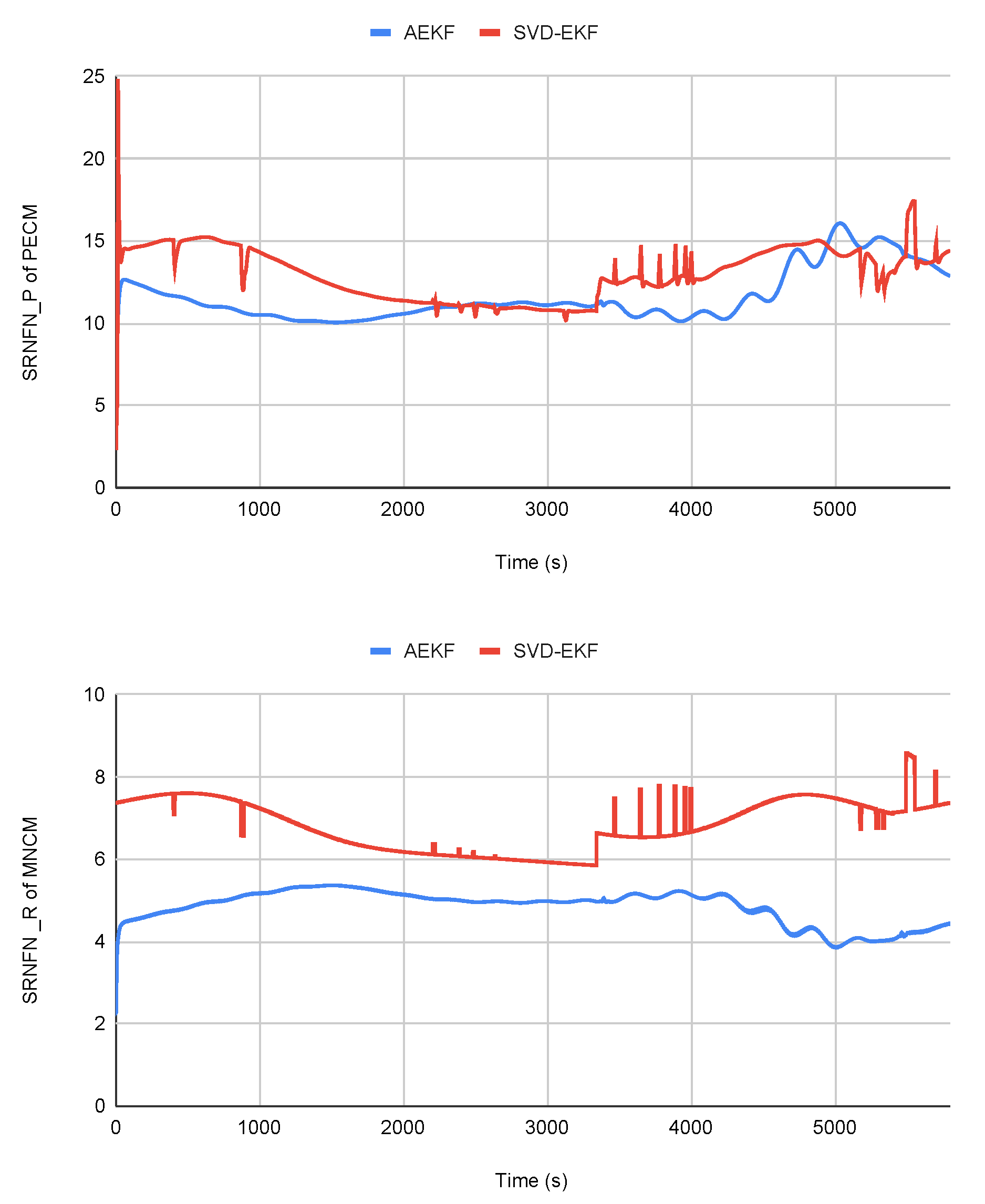
Figure 3.
SRNFN and SRNFN of the two filters during eclipse phase
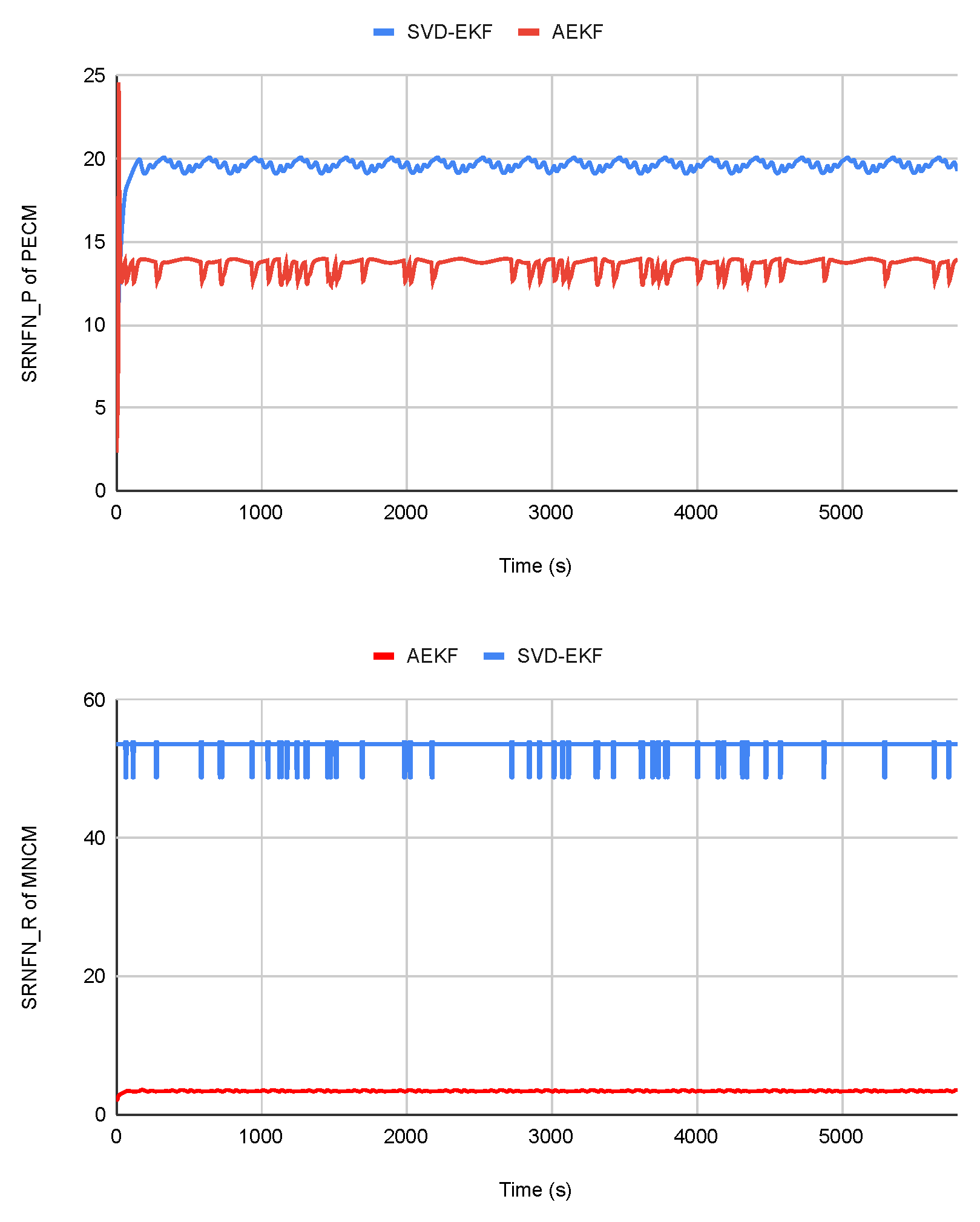

Table 1.
Comparison of the Root Mean Square Errors of the SVD-EKF and Proposed Algorithm During Sun Phase
Table 1.
Comparison of the Root Mean Square Errors of the SVD-EKF and Proposed Algorithm During Sun Phase
| RMSE | SVD-EKF | AEKF |
|---|---|---|
| 0.2146 | 0.0042 | |
| 0.2220 | 0.0015 | |
| 0.2472 | 0.0024 | |
| 3.6076e-06 | 4.4296e-08 | |
| 7.7722e-06 | 8.8530e-08 | |
| 8.8545e-06 | 1.7761e-08 |
Table 2.
Single Step Run Execution of the Proposed Algorithm and SVD-EKF
| Filters | SVD-EKF | AEKF |
|---|---|---|
| Time (s) | 7.94 | 8.46 |
Table 3.
Evaluation of the Proposed Algorithm and SVD-Aided EKF in Sunlit Phase using ASRNFN and ASRNFN
Table 3.
Evaluation of the Proposed Algorithm and SVD-Aided EKF in Sunlit Phase using ASRNFN and ASRNFN
| Filters | SVD-EKF | AEKF |
|---|---|---|
| ASRNFN | 13.0078 | 11.6005 |
| ASRNFN | 47.1554 | 4.8422 |
Table 4.
Comparison of the Root Mean Square Errors of the SVD-EKF and Proposed Algorithm During Eclipse Phase
Table 4.
Comparison of the Root Mean Square Errors of the SVD-EKF and Proposed Algorithm During Eclipse Phase
| RMSE | SVD-EKF | AEKF |
|---|---|---|
| 1.7126 | 0.1094 | |
| 12.6611 | 0.1388 | |
| 6.9083 | 0.3137 | |
| 7.9837e-05 | 1.3449e-07 | |
| 1.3499e-05 | 6.8046e-08 | |
| 1.9008e-04 | 1.8077e-08 |
Table 5.
Evaluation of the Proposed Algorithm and SVD-Aided EKF in Eclipse Phase using ASRNFN and ASRNFN
Table 5.
Evaluation of the Proposed Algorithm and SVD-Aided EKF in Eclipse Phase using ASRNFN and ASRNFN
| Filters | SVD-EKF | AEKF |
|---|---|---|
| ASRNFN | 19.5559 | 13.6083 |
| ASRNFN | 53.2372 | 3.4397 |
Disclaimer/Publisher’s Note: The statements, opinions and data contained in all publications are solely those of the individual author(s) and contributor(s) and not of MDPI and/or the editor(s). MDPI and/or the editor(s) disclaim responsibility for any injury to people or property resulting from any ideas, methods, instructions or products referred to in the content. |
© 2023 by the authors. Licensee MDPI, Basel, Switzerland. This article is an open access article distributed under the terms and conditions of the Creative Commons Attribution (CC BY) license (http://creativecommons.org/licenses/by/4.0/).
Copyright: This open access article is published under a Creative Commons CC BY 4.0 license, which permit the free download, distribution, and reuse, provided that the author and preprint are cited in any reuse.


