Submitted:
13 May 2023
Posted:
15 May 2023
You are already at the latest version
Abstract
This work presents a new scheme for autonomous control and obstacle detection of a catamaran unmanned surface vessel. Based on the Newtonian mechanics, hydrodynamics, and maneuvering modelling group modelling principles in the attached coordinate system, a three-degree-of-freedom motion model of the catamaran unmanned surface vessel is constructed. The fuzzy inference method is used to overcome the drawback that the traditional PID control cannot tune the PID parameters online, and the trajectory controller is designed. Meanwhile, 3D LIDAR is used to achieve obstacle detection. The results of the trajectory tracking simulations and experiments verify the accuracy of the model design and the effectiveness of the autonomous control design.
Keywords:
catamaran unmanned surface vessel
; maneuvering modeling group (MMG)
; fuzzy adaptive PID control
; obstacle detection
; trajectory tracking experiment
1. Introduction
Since the unmanned surface vessels (USVs) are cost-effective, flexible and fast, safe and reliable, small, intelligent, and able to cope with various climatic environments, USV will play an extremely important role in rivers, lakes and other environments as well as in the future military aspects of the sea [1,2]. The independent mathematical model of ship motion was proposed by the MMG group of the Japanese Towing Tank Conference (JTTC) [3]. Since the MMG model is physically easier to analyze and understand, it is more applicable to all types of USVs and its applications are more widespread. Xia et al. [4] only the horizontal maneuvering motion of the ship on still water was considered and the MMG model was used to analyze the forces on the rudder for the prediction of the maneuvering motion of a single ship. Reichel et al. [5] designed an MMG model to analyze and discuss the horizontal surface motion characteristics of a single USV with pod propulsion in order to quickly simulate the ship maneuverability. Chen et al. [6] developed a black box model of USV maneuvering motion with rudder angle and propeller speed based on the MMG model. Then, LS-SVM is used to identify the offline black box model and validate the motion prediction of USV. However, they only designed the online simulation framework in the simulation, which is still some distance from the experiment. More MMG models can be found in reference [7,8,9,10,11]. Therefore, the modeling idea of MMG is fully applicable to the USV of autonomous design. Trajectory tracking controllers commonly use PID control [7,12,13,14], Dong et al. [12] applied it to high-speed USV heading PD control by designing an improved bacteria foraging algorithm, which accelerated the convergence speed and improved the control accuracy; Horel et al. [13] studied the characteristics of rudder-controlled catamaran heading change based on a system approach. Ryoo et al. [15] used fuzzy control algorithm to achieve heading control with low accuracy. Wang et al. [16] created a finite-time fuzzy monocular vision servo scheme using adaptive fuzzy PID and adaptive residual feedback in the presence of unmeasurable attitude and velocity. In this paper, the fuzzy adaptive PID algorithm with simple structure and better robustness is considered for heading control design. Target detection is an important foundation for unmanned ships to achieve tasks such as obstacle avoidance and trajectory tracking. LIDAR was first applied to unmanned vehicles and other fields, and is commonly used for obstacle detection and environment map construction. With the development of USV technology, LIDAR is also applied to obstacle avoidance and other aspects in the field of unmanned ships [17,18,19]. Villa et al. [20] use LIDAR for navigation, control and obstacle avoidance and compute a predicted safety bounding box for each moving obstacle based on a system identification approach. Stateczny et al. [21] designed HydroDron, a universal autonomous control and management system for multipurpose USVs, which can also be used for tasks other than hydrographic surveys, such as monitoring rivers, lakes and other waters, environmental quality testing, etc.
This paper focuses on the design and engineering implementation of a catamaran USV system based on an attached coordinate system, MMG model and kinematic model with simplified degrees of freedom. A conventional PID controller is combined with fuzzy rules to achieve trajectory tracking under wind and wave disturbances. Path planning is accomplished by using differential GPS pre-targeting trajectories, and simulations and experimental results demonstrate the accuracy of the controller. The LIDAR acquires point cloud data, extends and erodes the obtained 3D point cloud data into the obstacle grid map and re-clusters it to complete the obstacle contour extraction and achieve simple obstacle avoidance.
The rest of the paper is organized as follows. Section II designs and improves the MMG model, and the data obtained from the velocity-thrust and rotational experiments are fitted to complete the parameter identification. Section III designs the path planning and trajectory tracking controller. The fuzzy adaptive PID controller is designed by establishing fuzzy rules and fuzzy affiliation functions. Section IV verifies the robustness of the fuzzy adaptive controller under wind and wave disturbances through simulation results. Section V verifies the effectiveness of the autonomous navigation and tracking system through experiments and implements the obstacle detection by LIDAR. Section VI summarizes the paper.
2. Motion Model and Parameter Identification of Vessel
The foundation of the investigation into USV motion modeling and control issues is the kinematic model. If the kinematic model is too exact, its equations of motion will invariably be nonlinear, the parameters will be tough to obtain, and it will be challenging to realize; if it is too basic, it will not accurately reflect the actual motion process of an USV, and the model will become meaningless. The kinematic analysis is divided into two aspects: from kinematic analysis, the catamaran USV is regarded as a mass point, and the relationship between its motion speed, heading angle and other variables and position is analyzed; from kinetic analysis, that is, the thrust of thrusters, fluid forces and interaction forces acting on the USV are studied. MMG model is suitable for self-research USV motion modeling analysis by virtue of its advantages of comprehensive force analysis and high flexibility.
2.1. MMG Motion Model
As shown in Figure 1, the USV in the water environment is generally described based on two coordinate systems [22]: the inertial coordinate system, i.e., the center point of the earth as the coordinate origin; and the attached coordinate system, i.e., the USV itself as the coordinate origin. The motion of the USV is divided into six states of motion with six degrees of freedom: displacement of the ship in the x, y and z axes, and rotation about the x, y and z axes. The USV motion state is represented in two different coordinate systems [22], and its transformation relationship is in (1):
where u and p represent the x-axis velocity and rotational angular velocity, v and q represent the y-axis velocity and rotational angular velocity, and w and r represent the z-axis velocity and rotational angular velocity. and represent transformation matrices, expressed in (2) and (3):
and
More detailed variable symbols are shown in Table 1.
Neglecting the longitudinal rotational angular velocity, transverse rotational angular velocity and the velocity of the USV along the z-axis in the water environment makes , , , , . The six-degree-of-freedom motion is simplified to a three-degree-of-freedom model, and the kinematic model is derived as (4) by combining (1), (2) and (3):
USVs are subjected to thrust of thrusters and drag of water, etc. when sailing in still waters. Each force and moment in the x-axis, y-axis and z-axes are shown in (5):
where denotes the hydrodynamic forces and moments acting on the hull and P denotes the hydrodynamic forces and moments of the thruster (thrust of the thruster). The forces and moments acting on the hull can be decomposed into inertial hydrodynamic forces, viscous hydrodynamic forces [23], as shown in (6):
where I denotes inertial fluid and H denotes viscous fluid.
When the origin of the attached coordinate system is at the center of mass of the USV, the equation of motion of the USV is as follows:
where m denotes the fully loaded mass of the USV, denotes the moment of inertia at the z axis, and N denotes the moment of momentum.
Assuming that the catamaran USV moves mainly on the stationary water surface, the three-degree-of-freedom equations of motion of the USV are obtained by combining (5), (6), and (7):
where P denotes dual propellers. Usually the viscous class fluid dynamics is much smaller than the other forces and can be neglected [24], so only the inertial class fluid dynamics and dual thruster dynamics are analyzed and calculated in this study.
The force generated by the surrounding fluid medium on the USV due to the perturbation caused by the USV during its navigation is called inertial class hydrodynamics. According to the velocity potential flow theory of the flow field, when the USV makes a variable speed motion in an ideal water environment, it generates a 6×6 attached mass inertia matrix m as (9):
Since the motion of the USV drives the motion of the surrounding fluid, the mass and moment of inertia of this fluid can be represented by the m-matrix, which is calculated as (10):
where represents the surface area of the waterline of the USV, represents the velocity potential in the direction of degree of freedom i, and n represents the normal vector.
For a fixed USV profile, the attachment inertia matrix is a constant independent of the motion variables. Since the object of study is based on symmetry in the x-o-z and x-o-y planes, for the 36 elements of the matrix, there are and only 8 independent non-zero elements, denoted as follows: (11):
where , , and are the attachment masses along the x, y, and z axes, respectively; , , and are the attachment moments of inertia in the x, y, and z axes, and and denote the attachment mass static moments, which are not zero because the y-o-z plane is not symmetric. The kinetic energy of the surrounding fluid flow caused by the motion of an unmanned vessel in a water environment can be expressed as (12):
where , , , , , , Substituting (11) into (12), we get
The momentum of the fluid perturbation motion is , and the fluid momentum and momentum moments projected on each coordinate axis can be expressed as (14)
where H denotes the fluid momentum and L denotes the fluid momentum moment.
Since the hydrodynamic force and the hydrodynamic moment , the expressions for the inertia-like hydrodynamic force and dynamic moment of the USV are obtained in (15):
According to the the motion of the USV with three degrees of freedom, namely longitudinal displacement, lateral displacement and bow rocking, is simplified and analyzed. Let , and , the expressions of inertia-like hydrodynamic forces and dynamic moments under the three-degree-of-freedom motion of the USV are obtained in (16):
There are two methods to calculate the attachment mass and the moment of inertia of the USV: the regression equation of Zhou et al. and the regression equation of Clarke et al. [25]. Zhou et al. performed a multiple regression analysis of the famous Motora’s atlas [26] as:
where B is the hull width, L is the unmanned vessel length, is the square factor, and d is the sea draught.
When the thruster rotates in a uniform water environment, its thrust and torque are related to the paddle diameter , forward velocity , water density , rotational speed n, water motion viscosity coefficient v, gravitational acceleration g, etc. According to the applied gauge analysis, the hydrodynamic force (thrust) of the thruster can be expressed as
Let , then we have:
Where, is the thrust coefficient. Similarly, the torque absorbed by the thruster, i.e., the reverse torque caused by the rotation of the water on the thruster, is found as
Let , then we have:
where is the torque coefficient. The thrust coefficient and torque coefficient are both correlation functions of the incoming speed coefficient . For the purpose of computer simulation, they can be expressed in the study of USV motion as
Where, , , and , , are the regression coefficients of the propeller open water characteristic curve [27]. The unmanned vessel is usually accompanied by slight rotational transport and lateral motion during the forward motion, and the effect of the latter two motions is usually summarized as the effect on the propulsion derating, i.e., the effect of the maneuvering motion on . The Norrbin model can be used [28]:
where B denotes the hull width, denotes the diameter of the propeller, denotes the longitudinal coordinates of the floating center, = -0.9L and using the Hankescher formula [29], for a double propeller boat, = 0.54, = 0.5-0.18, is the vessel’s rhombic coefficient, , and denotes the vessel immersion area.
The thrust from the thruster rotation is not all applied to the USV, part of it is the effective thrust, defined as , and the other part is used to overcome the drag increment caused by the thruster installed at the stern of the USV, defined as the thrust derating . In the practical engineering application of the USV, the dimensionless ratio of the thrust derating to the thruster thrust T is defined as the thrust derating factor , expressed as follows:
The USV traveling at low speed is approximately in uniform motion, so the effective thrust of a single thruster is equal to the drag R in (24), with
The combined thrust force of a catamaran unmanned vessel is expressed in the longitudinal direction as
where denotes the effective thrust of the left thruster and denotes the effective thrust of the right thruster. The twin thrusters produce torques
where denotes the distance from the two thrusters to the ship’s central axis.
The simplified dynamics model [30], analyzed by MMG modeling of the USV, is
where , is the velocity vector of the USV in three degrees of freedom; M is the inertial mass matrix of the USV; C is the centripetal and Koch force coefficient matrix; D denotes the drag coefficient matrix, and denotes the forces along the longitudinal and lateral directions of the thruster and the torque along the z axis direction, . According to [30], the coefficient matrix (28) is defined for each coefficient matrix as follows:
Based on the above analysis, a mathematical model of the three-degree-of-freedom motion of a twin-propulsion catamaran USV is established as shown below:
2.2. Parameter Identification
The mathematical model of three-degree-of-freedom motion of the catamaran is obtained according to the principle of MMG model, as shown in (30). The unknown parameters include inertial mass coefficient matrix M, centripetal force and Koch force coefficient matrix C, and drag coefficient matrix D. Among them, M and C can be calculated by physics equations according to the hull structure and weight; D needs to be identified by USV condition test data for parameter identification. Table 2 shows the basic USV parameters.
According to the basic parameters in Table 2, . Bringing into equation (17), it is calculated according to [30] that , , .
In (29), , , . The relationship between the thrust of the USV thruster and the speed of the USV is difficult to be found by the theoretical formula, and the parameters of the matrix D are identified by experimental data in this study.
In the control system designed in this paper, the output power of the thruster is controlled by setting the control code n (0→120), which corresponds to the input control voltage of the thruster (0V→5V). For a single thruster, the linear relationship between and the voltage interval is
The change in thruster control voltage in turn affects the thrust applied to the USV. According to the thruster data sheet, the relationship between individual thruster thrust and the controlled voltage is as follows:
The forward direction of the USV is subject to the combined thrust force of the dual thrusters as and the torque . Therefore, when the left and right thrusters have the same speed, the relationship between the control code n and the combined thrust force can be obtained by substituting (31) into (32) as follows:
The experimental data were fitted to the relationship between the combined thrust force and the velocity using Matlab, and the linear relationship was obtained as shown in Figure 2.
The linear relationship between the velocity and the combined thrust force is obtained by fitting: . Therefore, . When the left and right thrusters rotate at different speeds, the dual thrusters do slewing motion with torque , and similarly, , as shown in Figure 3. Therefore, the mathematical model of the motion of the dual-propulsion catamaran is obtained as shown in (34).
In order to verify the accuracy of the model constructed in this paper, the motion model is designed for slewing motion simulation using Matlab tools, and compared with the USV in the real water environment for slewing motion test to verify. The left and right thruster control codes are set to 20 and 15 respectively, the initial speed is 0 m/s, and the initial heading angle is 0. After stabilization, the speed is 0.209 m/s, and the simulation result of slewing motion is shown in Figure 3, and the calculated slewing diameter is about 7.38 m.
The test environment had a light wind, the control codes of the left and right thrusters of the USV were given as 20 and 15 respectively, the speed was about 0.246 m/s, three sets of slewing motion were completed, the software platform of the USV collected the longitude and latitude information to generate data tables, and Matlab was used to plot the slewing motion trajectory in the water environment as shown in Figure 4, and the calculated slewing diameter was about 8 m.
Comprehensive analysis of Figure 3 and Figure 4 shows that the simulation results of the gyratory motion of the USV are consistent with its gyratory motion in the real water environment, which indicates that the motion model of the twin-thruster USV in this paper is more compatible with the real catamaran USV.
3. Trajectory Control
The GPS can provide real-time feedback of latitude and longitude information and heading angle of the current position of the unmanned vessel, so the current angle to be tracked can be obtained by calculating the azimuth angle, and the track point tracking can be realized according to the distance between the current position and the target point. Azimuth angle and distance between two points: Let the current position of the USV , the next target point position , and the current heading angle calculation equation are shown in (35):
where denote the latitude of positions A and B, denote the longitude of positions A and B, and denotes the latitude correction.
Since the length of the latitudinal circle on the earth’s surface changes with latitude, the error in the calculation directly using the Pythagorean theorem is too large. According to [31], the distance between two points A and B is calculated as (36):
where the radius of the Earth km.
Trajectory tracking controller with incremental PID control [15]:
Using the incremental PID algorithm to correct the deviation of the current heading angle from the target heading angle, the heading control equation is in (38):
In order to improve the control performance of the heading controller, the PID control with high accuracy is combined with the fuzzy control algorithm with high robustness to overcome the shortcomings of the traditional PID parameters that cannot adjust the PID parameters in real time.
From Figure 5 , the deviation e and the variation of the deviation are the inputs to the fuzzy adaptive controller, and the PID controller parameters are adjusted using the output values determined by fuzzy judgments as the adjustment of the proportional, integral, and differential coefficients [32], with the following expressions:
where , , and are the reference values, and , , and are the adjustment amounts obtained by the fuzzy adaptive controller.
The heading fuzzy adaptive PID controller has two input variables: heading deviation e and the rate of change of heading deviation . The actual ranges of the two input variables are converted into the corresponding fuzzy theoretical domains E and , while , , and in the fuzzy adaptive PID control algorithm are used as the fuzzy adaptive controller outputs, and the five variable output domains are all designed as , respectively. Considering the influence of the number of fuzzy subsets on the accuracy of unmanned ship heading control, each fuzzy theoretical domain is quantified into seven classes, which are negative large (NB), negative medium (NM), negative small (NS), zero (Z), positive small (PS), positive medium (PM), and positive large (PB). Each subset needs to be described by the affiliation function, and the more gentle S function and Z function are used in the larger input region to improve the stability, while the more sharp triangular function is chosen in the smaller input region to improve the sensitivity, and the mathematical principle expression is as (40):
where x is used to specify the range of the domain of the variable, and the parameters a, b, and c specify the shape of the triangular function. In this paper, we design the affiliation functions of E, , , , and as shown in Figure 6.
, and in the fuzzy adaptive PID control algorithm can be adjusted under different heading deviation e and heading deviation change rate according to the following Table 3, Table 4 and Table 5.
In Table 3, when the value of is small, the actual heading of the USV is close to the set heading value. At this time, if the value of is small, a larger and a moderate should be taken in order to make the system reach the steady state faster; if the value of is large, a smaller and should be taken in order to prevent the system from overshooting too much.
In Table 4, when , value is moderate, in order to reduce the amount of system overshoot, value should be taken smaller, while considering the response speed of the controlled system, , value should be moderate.
In Table 5, when the value of is large, the value of should be larger to ensure the rapidity of the system response, and the value of should be close to zero and the value of should be smaller to strengthen the suppression of overshoot.
The formula for the weighted average method of defuzzification is , where u is the exact value of the defuzzy output, is the subset of the output fuzzy domain, and is the affiliation degree corresponding to the output subset.
4. Simulation Results
Under the action of no disturbing force, PID simulation and fuzzy adaptive PID simulation are performed on the USV dynamics model, setting the initial angle of the USV 0, the starting point position (0, 0), and the azimuth angle is calculated as 74 according to the tracking track point (70, 20), and the dual thruster control volume change curve and heading angle adjustment curve are shown in Figure 7.
From Figure 7, it can be seen that the PID control effect is slightly inferior to the fuzzy adaptive PID control effect under the effect of no external disturbance.
In order to more realistically describe the heading control performance of an unmanned vessel in real waters, the effect of wind and wave disturbance is added to the simulation, and a linear wind and wave model is used instead of a complex nonlinear wind and wave model [33,34], and the linear wind and wave model expression is approximated as follows:
where denotes Gaussian white noise with zero mean and power spectral density of 0.1, and denotes the second-order wave transfer function with the following expressions:
where denotes the dominant wave frequency, denotes the damping coefficient, denotes the gain constant, and denotes the wave intensity. The simulation environment is set as wind level four with small waves, with =0.20, =0.54 and =0.61.
Under the action of wind and wave disturbance force, PID simulation and fuzzy adaptive PID simulation are carried out for the USV dynamics model. The initial angle of the USV is set to 0, the starting point position (0, 0), and the azimuth angle is calculated as 74 according to the tracking track point (70, 20), and the change curve of the dual thruster control volume and heading angle adjustment curve are shown in Figure 8, and the fuzzy adaptive controller adjusts the , and parameters in real time as shown in Figure 9.
The simulation results show that the closed-loop system with fuzzy adaptive PID controller has improved response time, overshoot, and dynamic performance compared with the conventional PID controller with the same initial parameters, especially in the case of disturbances.
Further, track point tracking simulation is performed. The starting point is set to point (100, 100), the starting heading is 90, with five tracking points (200, 200), (300, 200), (400, 300), (500, 300), (600, 400), and the simulation results are shown in Figure 10.
As shown in Figure 10, with the effect of wind and wave disturbance, the track error accumulates under the PID control, and converges and remains stable after the fuzzy adaptive PID regulation, indicating that the track point tracking based on the fuzzy adaptive PID machine is better than that of the PID controller.
5. Analysis of Experimental Results
During the sailing of the USV, the 4G router and differential GPS are used to obtain information such as latitude and longitude, sailing speed, current heading angle, etc. The software platform control system is built on the IPC to correct the error angle in real time and send control commands to the microcontroller to control the left and right propellers respectively to achieve heading control and track point tracking, and the sailing test is shown in Figure 11.
The designed catamaran USV consists of two 450W propeller thrusters, thruster controller, IPC, differential GPS, 4G router and power supply system, the external design is shown in Figure 12 and the internal design is shown in Figure 13.
The GPS data sheet of the pre-navigation track was collected in advance, and the coordinates (30°46’21.6403 "N, 104°58’48.6782 "E) were used as the starting point in this latitude and longitude range, and the starting heading was 270°, and eight track points to be tracked were selected, as shown in Figure 11 and Table 6.
As shown in Figure 14. The test results show that the differential propulsion catamaran designed independently in this paper has completed the track point tracking in the lake. The test results fully verify the accuracy of the fuzzy adaptive PID heading controller.
5.1. Obstacle Detection
By acquiring point cloud data through 3D LiDAR, the original data obtained from the scan is under the spherical coordinate system, which is converted to the attached coordinate system for the convenience of subsequent data processing and use (43):
where denotes the position point information under the attached coordinate system, R denotes the distance of the scanning point from the LIDAR, denotes the pitch angle of the scan line where the point is located, denotes the heading angle in the horizontal direction, and , and denote the displacement of the origin of the attached coordinate system relative to the origin of the coordinate system where the point cloud data is located in the X, Y and Z directions, respectively.
According to the height of the USV and the installation position of LiDAR, this paper establishes the right-hand coordinate system with LiDAR as the coordinate origin, sets the 3D points with z-value greater than 1 meter as unnecessary point cloud data, and completes the shore point cloud data filtering by z-value filtering method, and the comparison before and after processing is shown in Figure 15. It can be seen from the figure that the amount of point cloud data is obviously reduced.
When there are multiple points, the maximum relative height difference is obtained by counting the highest value and the lowest value in the raster, and if the difference is greater than the threshold n, the raster is marked as an obstacle point. This relative height difference calculation method effectively reduces the errors caused by the horizontal and vertical rocking motion of the USV and the water surface trash on the point cloud data.
The processing results are obtained as shown in Figure 16. From Figure 5 and Figure 6, it can be seen that the raster attributes are determined by z-value filtering method and threshold segmentation method, and finally the obstacle raster map is obtained as Figure 16 (b), compared with Figure 16 (a), the unnecessary point cloud data is effectively reduced without affecting the main obstacle structure information.
The raster processed data are all discrete points, and there are isolated points collected under the influence of variable environment in some of the raster, so in order to filter out the isolated points and connect the neighboring points at the same time, the expansion corrosion operation is used to achieve clustering and contour extraction.
Based on the above method for contour extraction of the top view, and the detection results are shown in Figure 17 after the expansion and erosion process of the obstacle raster map. According to the USV raster coordinates , it can be seen that the box marked as 4 in Figure 17 (a) is the obstacle ship. From Figure 17, it can be seen that when the minimum value of rectangular box sizemin is obtained larger, the missed detection may occur, such as the obstacle marked as 1 in Figure 17 (a) is not detected. Therefore, the design takes sizemin to ensure the effectiveness of obstacle detection.
6. Conclusions
In this work, a new three-degree-of-freedom unmanned boat model based on the MMG model is proposed. Different from the usual USV dynamics model [22], the hydrodynamics and Newtonian mechanics of the two-thruster catamaran USV are considered, and the unknown parameters are identified by velocity-thrust experiments and rotational motion experiments. In addition, PID heading controller and fuzzy adaptive PID heading controller are designed, and the better effect of fuzzy adaptive PID heading controller in the presence of disturbance is proved by simulation analysis and experimental data, and the trajectory point tracking experiment is designed on this basis, and the accuracy of the heading controller is verified by simulation and verification. Further, the obstacle detection is realized by using 3D LiDAR, and the obstacle contour extraction is completed by filtering and re-clustering the point cloud map. In our future work, we will focus on the collision avoidance control of USV motion in complex scenes, which is challenging under uncertain disturbances and strong nonlinear dynamics [35,36].
Author Contributions
Methodology, T.R. and D.W; Project administration, Y.Z; Software, D.W; Supervision, Y.Z; Validation, T.R. and D.W; Visualization, D.W; Writing – original draft, T.R; Writing – review & editing, T.R and Y.Z. All authors have read and agreed to the published version of the manuscript.
Funding
This research received no external funding.
Data Availability Statement
The data presented in this study are available upon request from the corresponding author.
Conflicts of Interest
The authors declare no conflict of interest.
References
- Barrera, C.; Padron, I.; Luis, F.; Llinas, O. Trends and challenges in unmanned surface vehicles (Usv): From survey to shipping. TransNav: International Journal on Marine Navigation and Safety of Sea Transportation 2021, 15. [Google Scholar] [CrossRef]
- Mousazadeh, H.; Jafarbiglu, H.; Abdolmaleki, H.; Omrani, E.; Monhaseri, F.; Abdollahzadeh, M.r.; Mohammadi-Aghdam, A.; Kiapei, A.; Salmani-Zakaria, Y.; Makhsoos, A. Developing a navigation, guidance and obstacle avoidance algorithm for an Unmanned Surface Vehicle (USV) by algorithms fusion. Ocean Engineering 2018, 159, 56–65. [Google Scholar] [CrossRef]
- Yasukawa, H.; Yoshimura, Y. Introduction of MMG standard method for ship maneuvering predictions. Journal of marine science and technology 2015, 20, 37–52. [Google Scholar] [CrossRef]
- Xia, Y.; Zheng, S.; Yang, Y.; Qu, Z. Ship Maneuvering Performance Prediction Based on MMG Model. IOP Conf. Ser.: Mater. Sci. Eng. 2018, 452, 042046. [Google Scholar] [CrossRef]
- Reichel, M. Prediction of manoeuvring abilities of 10000 DWT pod-driven coastal tanker. Ocean Eng. 2017, 136, 201–208. [Google Scholar] [CrossRef]
- Chen, L.; Yang, P.; Li, S.; Liu, K.; Wang, K.; Zhou, X. Online modeling and prediction of maritime autonomous surface ship maneuvering motion under ocean waves. Ocean Engineering 2023, 276, 114183. [Google Scholar] [CrossRef]
- Peng, Y.; Yang, Y.; Cui, J.; Li, X.; Pu, H.; Gu, J.; Xie, S.; Luo, J. Development of the USV ‘JingHai-I’and sea trials in the Southern Yellow Sea. Ocean engineering 2017, 131, 186–196. [Google Scholar] [CrossRef]
- Lopes, P.; da Pires, P.S.; Moreira, M. Design Challenges of a Maritime Multipurpose Unmanned Vehicle. IOP Conf. Ser.: Earth Environ. Sci. 2018, 172, 012024. [Google Scholar] [CrossRef]
- Li, M.; Mou, J.; Chen, L.; Huang, Y.; Chen, P. Comparison between the collision avoidance decision-making in theoretical research and navigation practices. Ocean Eng. 2021, 228, 108881. [Google Scholar] [CrossRef]
- Sukas, O.F.; Kinaci, O.K.; Bal, S. System-based prediction of maneuvering performance of twin-propeller and twin-rudder ship using a modular mathematical model. Appl. Ocean Res. 2019, 84, 145–162. [Google Scholar] [CrossRef]
- Peeters, G.; Boonen, R.; Vanierschot, M.; DeFilippo, M.; Robinette, P.; Slaets, P. Asymmetric Steering Hydrodynamics Identification of a Differential Drive Unmanned Surface Vessel⁎⁎This research was funded by Flanders Research Foundation. IFAC-PapersOnLine 2018, 51, 207–212, 11th IFAC Conference on Control Applications in Marine Systems, Robotics, and Vehicles CAMS 2018. [Google Scholar] [CrossRef]
- Dong, Z.; Bao, T.; Zheng, M.; Yang, X.; Song, L.; Mao, Y. Heading control of unmanned marine vehicles based on an improved robust adaptive fuzzy neural network control algorithm. IEEE Access 2019, 7, 9704–9713. [Google Scholar] [CrossRef]
- Horel, B. System-based modelling of a foiling catamaran. Ocean Eng. 2019, 171, 108–119. [Google Scholar] [CrossRef]
- Zhu, Q. Design of control system of USV based on double propellers. 2013 IEEE International Conference of IEEE Region 10 (TENCON 2013), 2013, pp. 1–4. [CrossRef]
- Ryoo, Y.J.; others. An autonomous control of fuzzy-PD controller for quadcopter. International Journal of Fuzzy Logic and Intelligent Systems 2017, 17, 107–113. [Google Scholar]
- Wang, N.; He, H. Dynamics-level finite-time fuzzy monocular visual servo of an unmanned surface vehicle. IEEE Transactions on Industrial Electronics 2019, 67, 9648–9658. [Google Scholar] [CrossRef]
- Villa, J.L.; Paez, J.; Quintero, C.; Yime, E.; Cabrera, J. Design and control of an unmanned surface vehicle for environmental monitoring applications. 2016 IEEE Colombian Conference on Robotics and Automation (CCRA), 2016, pp. 1–5. [CrossRef]
- Asvadi, A.; Premebida, C.; Peixoto, P.; Nunes, U. 3D Lidar-based static and moving obstacle detection in driving environments: An approach based on voxels and multi-region ground planes. Robot. Auton. Syst. 2016, 83, 299–311. [Google Scholar] [CrossRef]
- Pouliot, N.; Richard, P.L.; Montambault, S. LineScout power line robot: Characterization of a UTM-30LX LIDAR system for obstacle detection. 2012 IEEE/RSJ International Conference on Intelligent Robots and Systems, 2012, pp. 4327–4334. [CrossRef]
- Villa, J.; Aaltonen, J.; Koskinen, K.T. Path-following with lidar-based obstacle avoidance of an unmanned surface vehicle in harbor conditions. IEEE/ASME Transactions on Mechatronics 2020, 25, 1812–1820. [Google Scholar] [CrossRef]
- Stateczny, A.; Burdziakowski, P. Universal autonomous control and management system for multipurpose unmanned surface vessel. Polish Maritime Research 2019, 26, 30–39. [Google Scholar] [CrossRef]
- Goldfain, B.; Drews, P.; You, C.; Barulic, M.; Velev, O.; Tsiotras, P.; Rehg, J.M. Autorally: An open platform for aggressive autonomous driving. IEEE Control Syst. Mag. 2019, 39, 26–55. [Google Scholar] [CrossRef]
- Wu, J.; Yang, X.; Xu, S.; Han, X. Numerical investigation on underwater towed system dynamics using a novel hydrodynamic model. Ocean Engineering 2022, 247, 110632. [Google Scholar] [CrossRef]
- Tao, Z.; You, R.; Ma, Y.; Li, H. Temperature and velocity characteristics of rotating turbulent boundary layers under non-isothermal conditions. Physics of Fluids 2022, 34, 065138. [Google Scholar] [CrossRef]
- Qi, J.; Wang, B.; Fei, Q. Curve Path Following Based on Improved Line-of-Sight Algorithm for USV. 2022 China Automation Congress (CAC). IEEE, 2022, pp. 3801–3806.
- Motora, S. On the measurement of added mass and added moment of inertia for ship motions Part 2. Added mass Abstract for the longitudinal motions. Journal of Zosen Kiokai 1960, 1960, a59–a62. [Google Scholar] [CrossRef]
- Han, J.; Cho, Y.; Kim, J. Coastal SLAM with marine radar for USV operation in GPS-restricted situations. IEEE Journal of Oceanic Engineering 2019, 44, 300–309. [Google Scholar] [CrossRef]
- Norrbin, N.H. Theory and Observation on the Use of a Mathematical Model for Ship Maneuvering in Deep and Confined Water. Proc. 8th Symposium on naval Hydrodynamics, 1977.
- Guo, M.; Guo, C.; Zhang, C.; Zhang, D.; Gao, Z. Fusion of ship perceptual information for electronic navigational chart and radar images based on deep learning. The Journal of Navigation 2020, 73, 192–211. [Google Scholar] [CrossRef]
- Fossen, T.I. Handbook of marine craft hydrodynamics and motion control; John Wiley & Sons, 2011.
- Fossen, T.I.; Breivik, M.; Skjetne, R. Line-of-sight path following of underactuated marine craft. IFAC Proceedings Volumes 2003, 36, 211–216, 6th IFAC Conference on Manoeuvring and Control of Marine Craft (MCMC 2003), Girona, Spain, 17-19 September, 1997. [Google Scholar] [CrossRef]
- Ghamari, S.M.; Narm, H.G.; Mollaee, H. Fractional-order fuzzy PID controller design on buck converter with antlion optimization algorithm. IET Control Theory & Applications 2022, 16, 340–352. [Google Scholar]
- Leng, J.; Wang, Q.; Li, Y. A geometrically nonlinear analysis method for offshore renewable energy systems—Examples of offshore wind and wave devices. Ocean Engineering 2022, 250, 110930. [Google Scholar] [CrossRef]
- Basbas, H.; Liu, Y.C.; Laghrouche, S.; Hilairet, M.; Plestan, F. Review on Floating Offshore Wind Turbine Models for Nonlinear Control Design. Energies 2022, 15, 5477. [Google Scholar] [CrossRef]
- Guo, X.G.; Xu, W.D.; Wang, J.L.; Park, J.H.; Yan, H. BLF-based neuroadaptive fault-tolerant control for nonlinear vehicular platoon with time-varying fault directions and distance restrictions. IEEE Transactions on Intelligent Transportation Systems 2021, 23, 12388–12398. [Google Scholar] [CrossRef]
- Xiong, Z.; Liu, Z.; Luo, Y. Formation tracking of underactuated unmanned surface vehicles with connectivity maintenance and collision avoidance under velocity constraints. Ocean Engineering 2022, 265, 112698. [Google Scholar] [CrossRef]
Figure 1.
Definition of coordinate system and vessel motions.
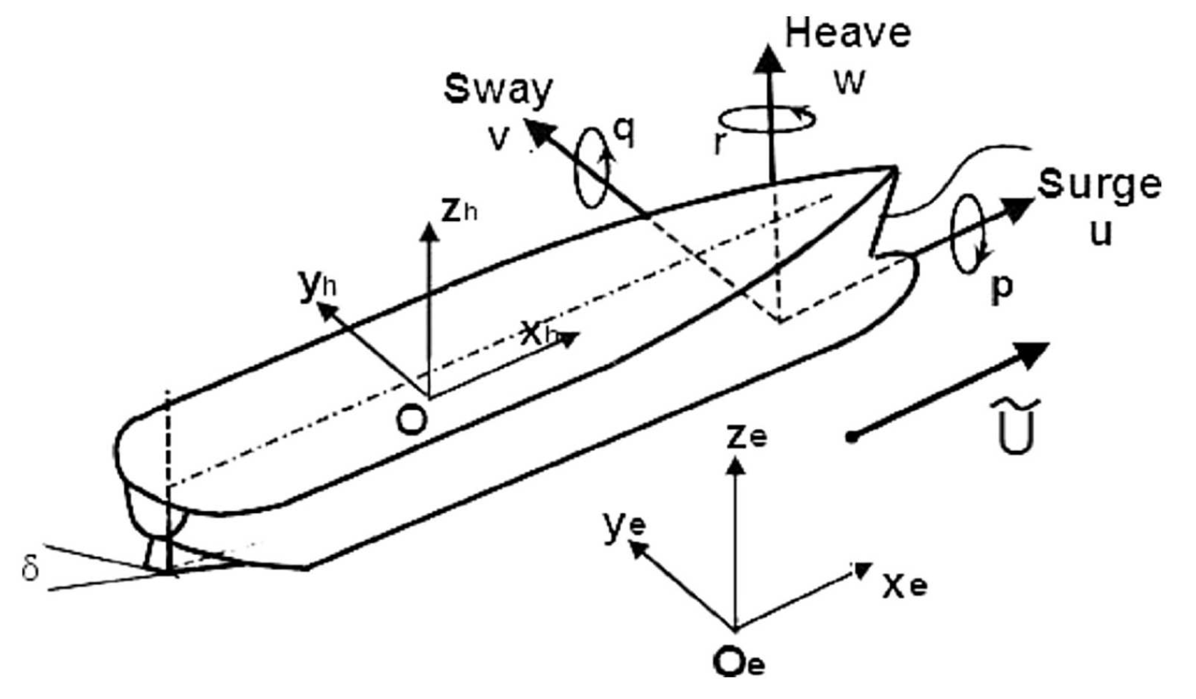
Figure 2.
Fitted curve of velocity-thrust.
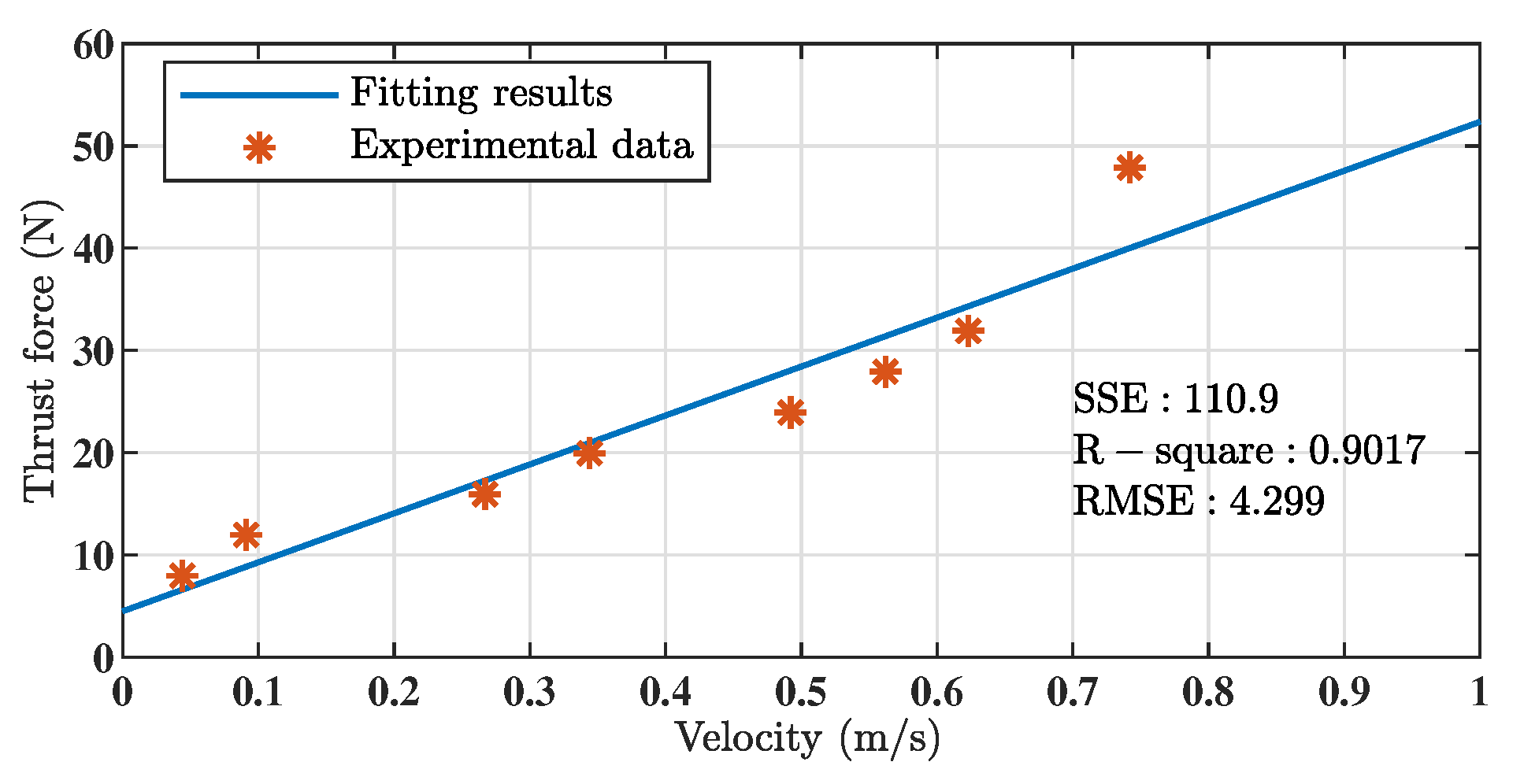
Figure 3.
Rotational motion simulation results.
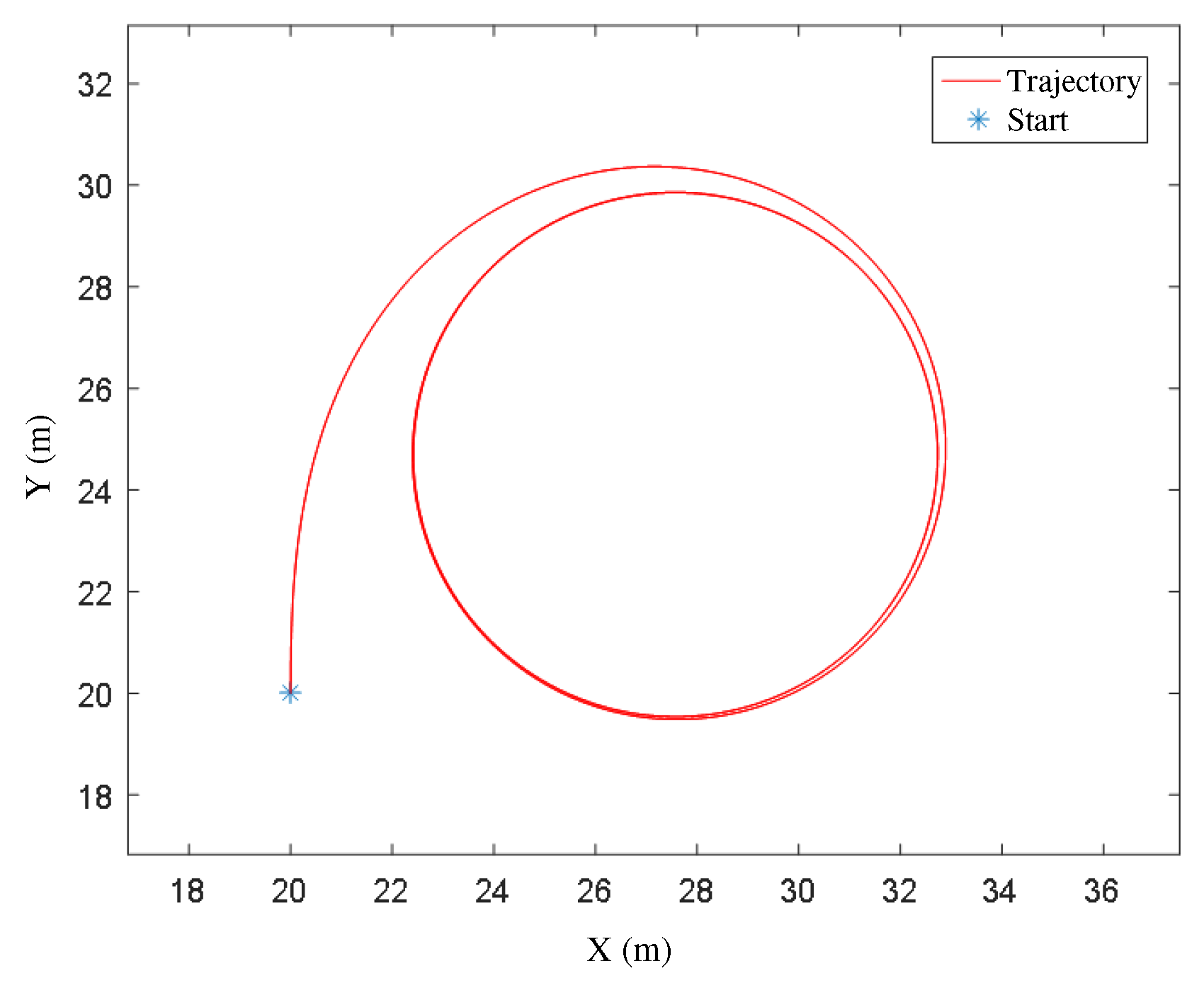
Figure 4.
Experimental results of rotary motion.
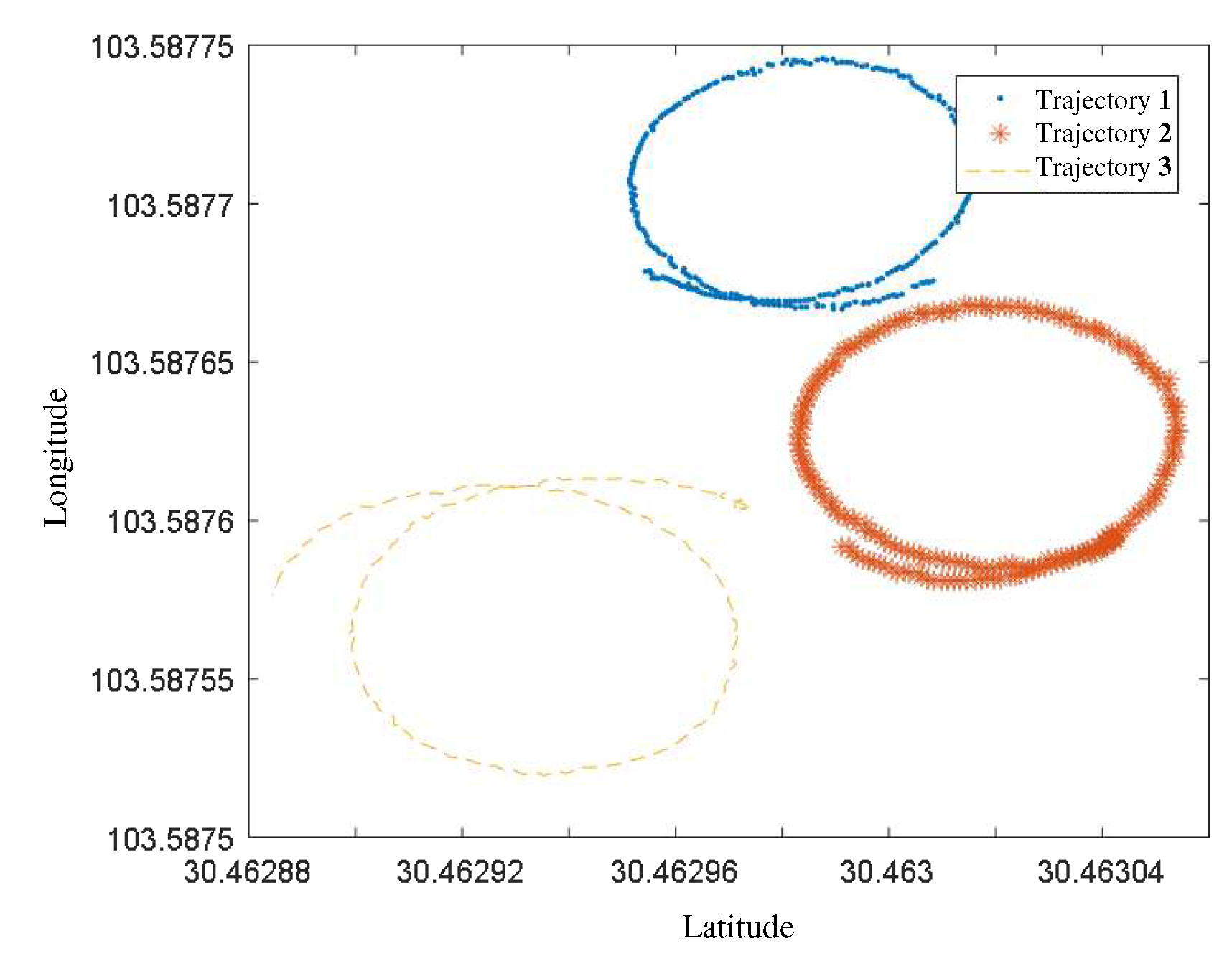
Figure 5.
Fuzzy adaptive PID control system structure.
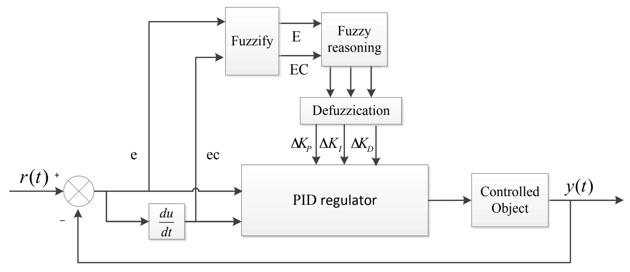
Figure 6.
Affiliation functions of E, , , , .
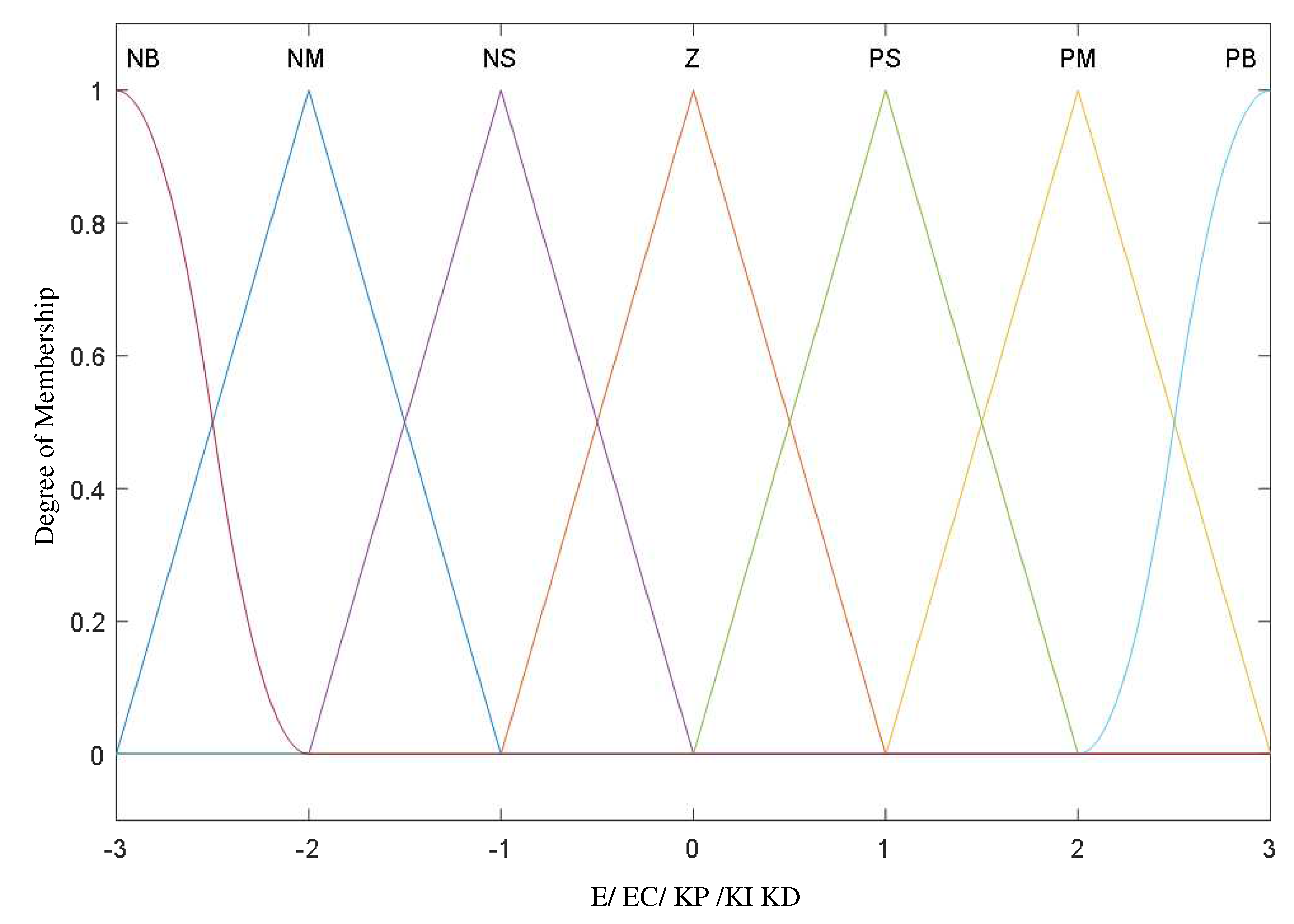
Figure 7.
Simulation curves of PID control and fuzzy adaptive PID control trajectory under no disturbance.
Figure 7.
Simulation curves of PID control and fuzzy adaptive PID control trajectory under no disturbance.
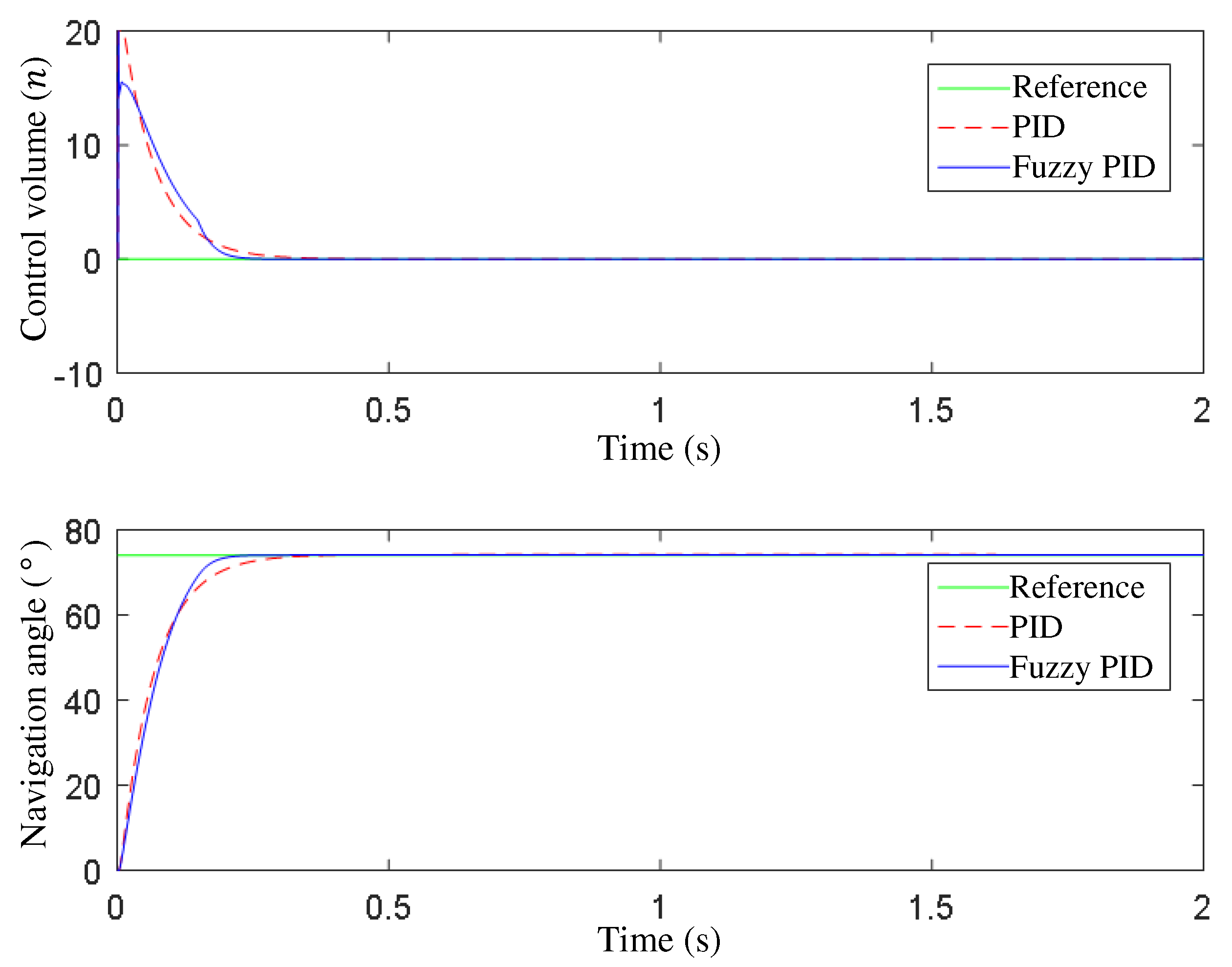
Figure 8.
Simulation curves of PID control and fuzzy adaptive PID control trajectory under wind and wave disturbances.
Figure 8.
Simulation curves of PID control and fuzzy adaptive PID control trajectory under wind and wave disturbances.
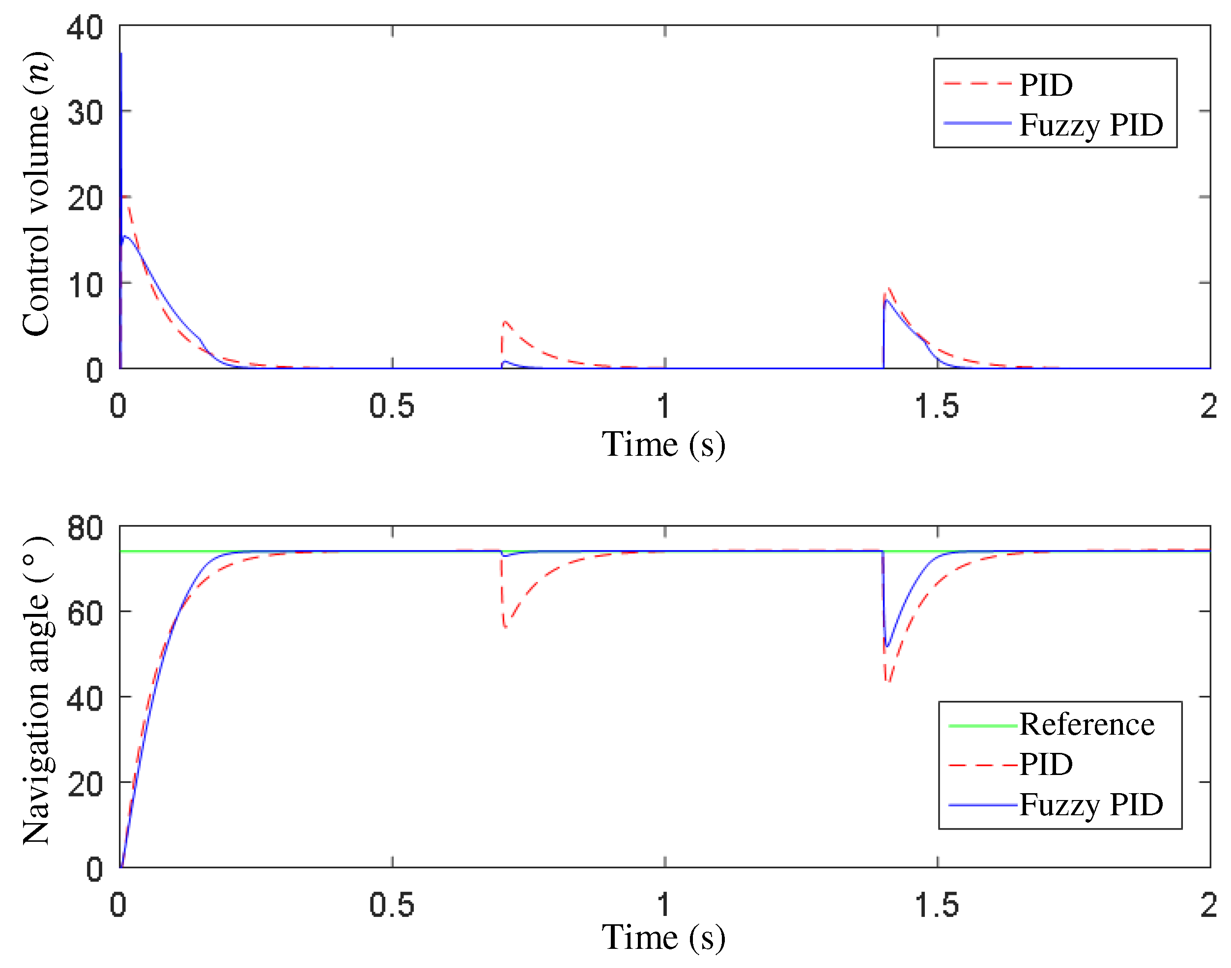
Figure 9.
Parameter tuning curves of , , under wind and wave disturbances.
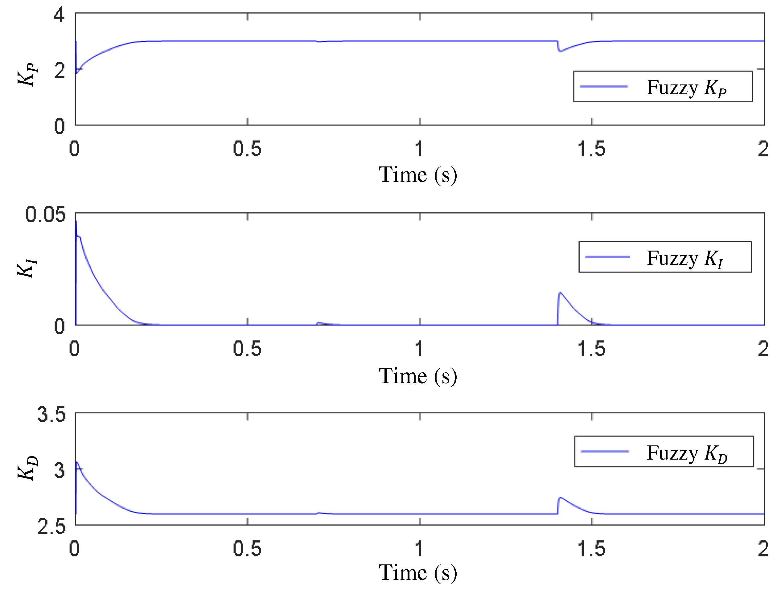
Figure 10.
Simulation of multi-track point tracking under PID and fuzzy adaptive PID.
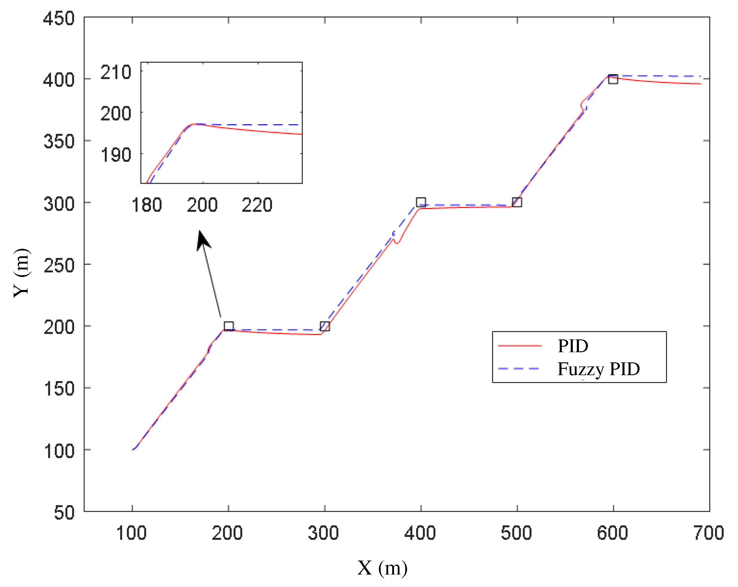
Figure 11.
Visualization upper computer software platform.
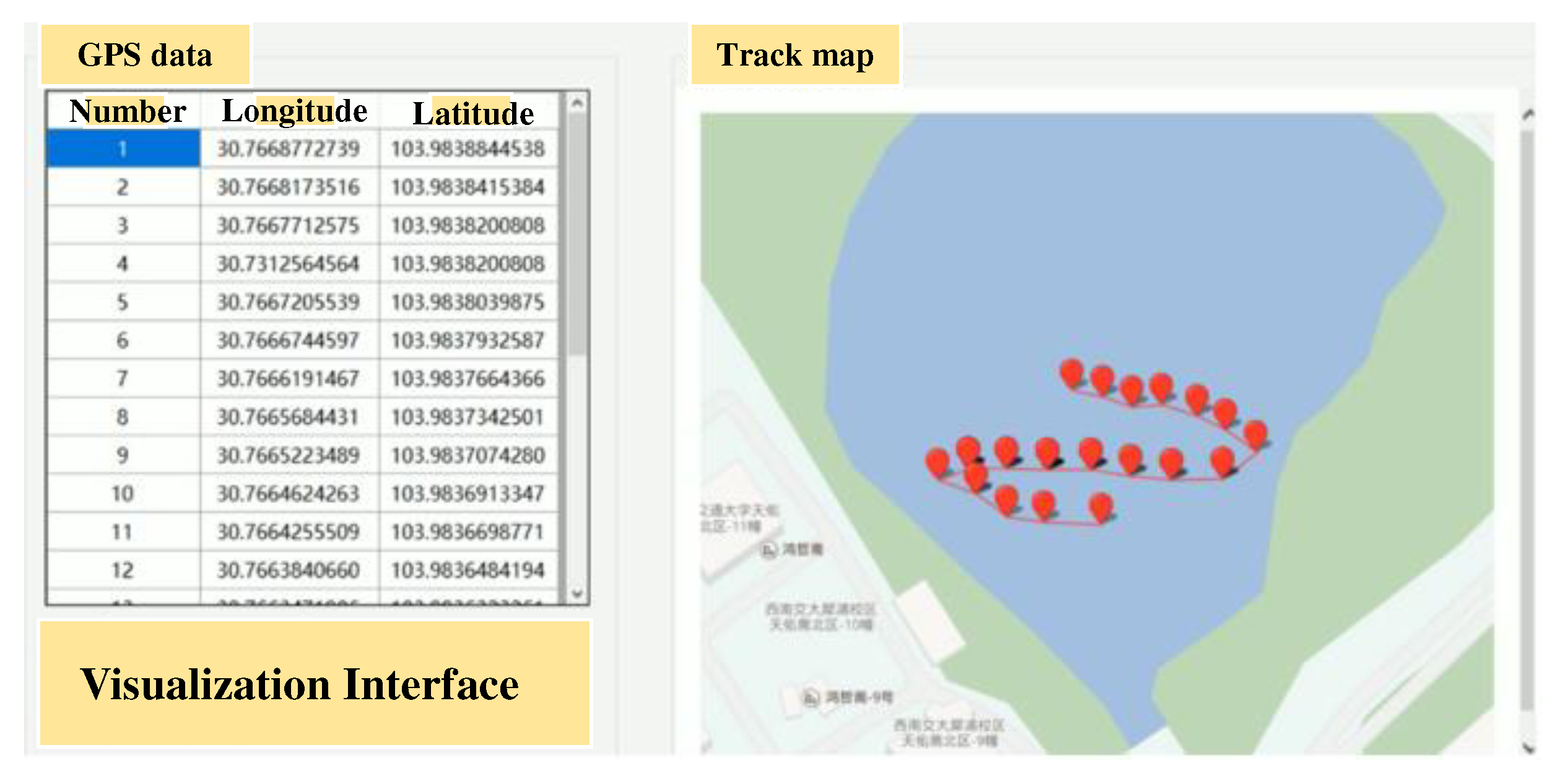
Figure 12.
Physical picture of the vessel.
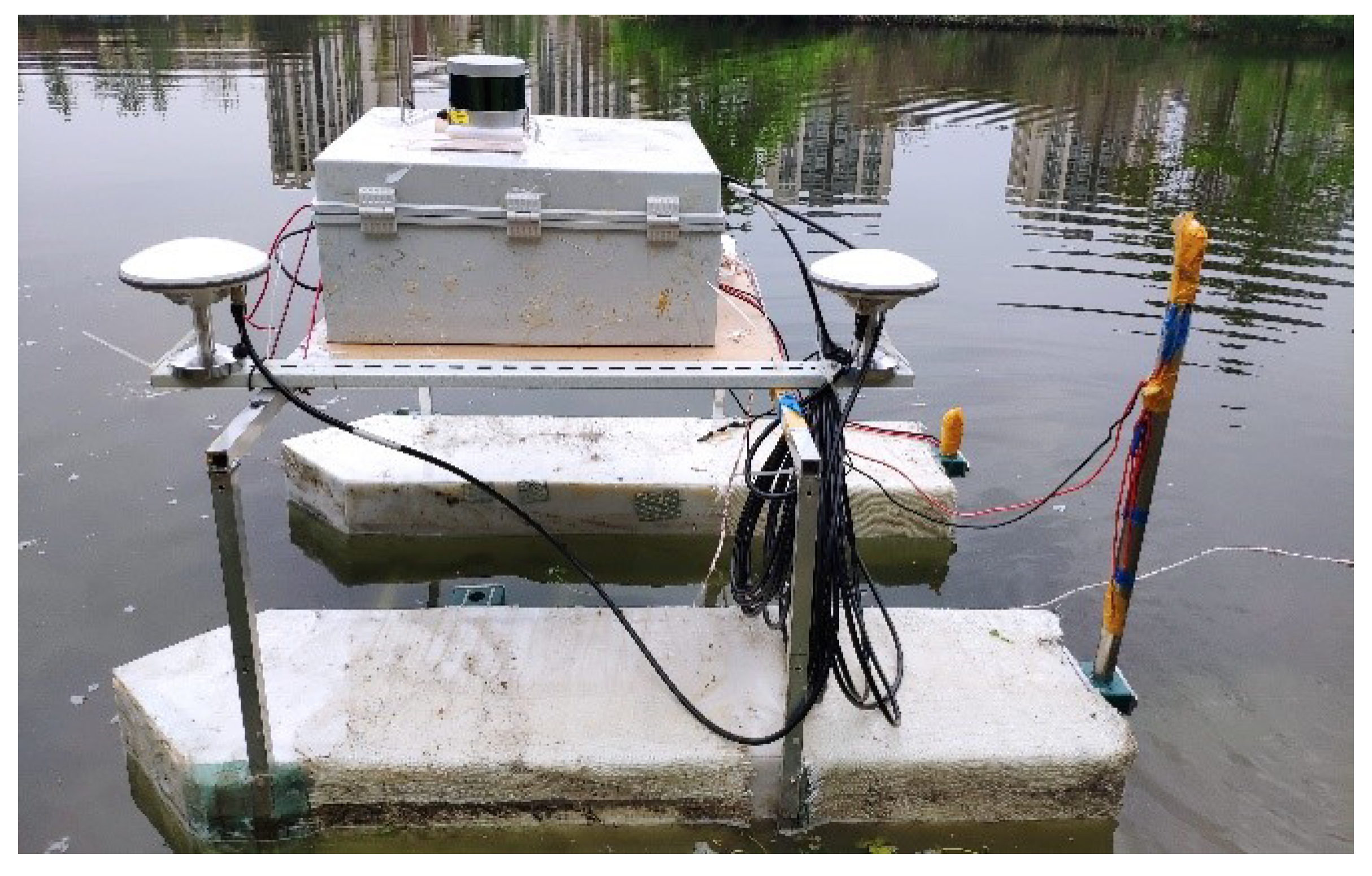
Figure 13.
Equipment box internal diagram.
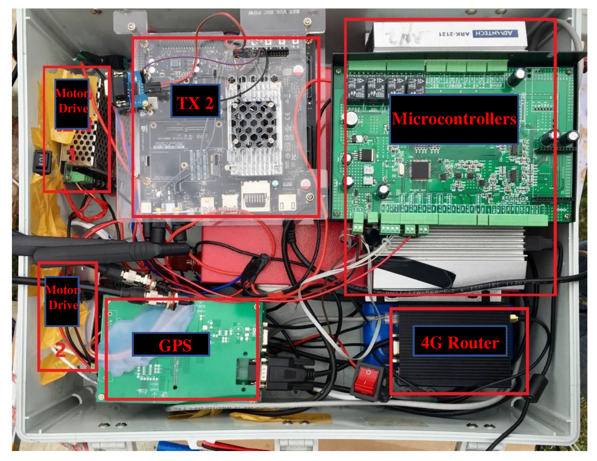
Figure 14.
Track-tracking experiments of a catamaran USV.
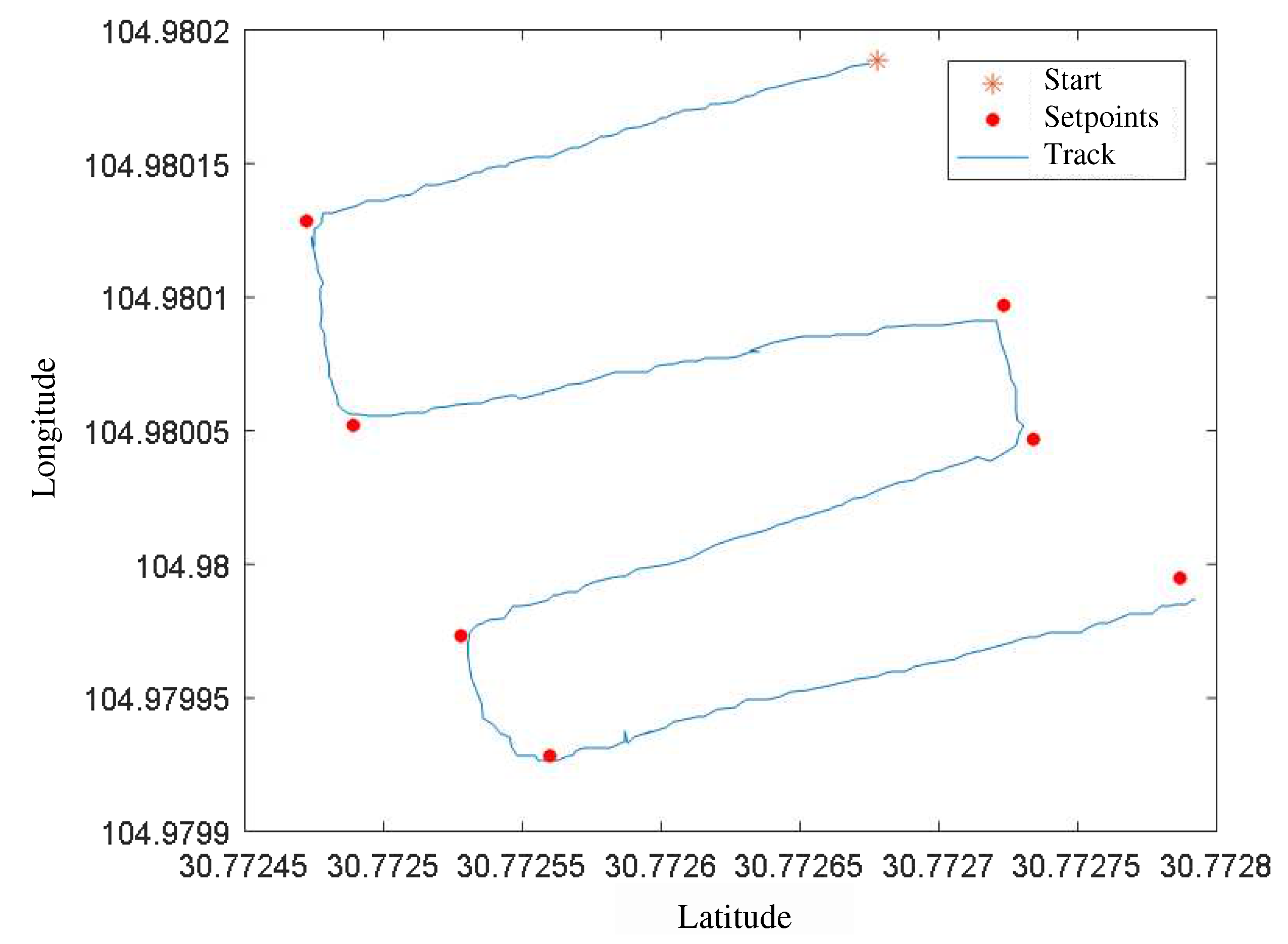
Figure 15.
Comparison of shore point cloud data before and after filtering: (a) . (b) .

Figure 16.
Comparison of original map and obstacle grid map: (a) Original map. (b) Obstacle grid map.
Figure 16.
Comparison of original map and obstacle grid map: (a) Original map. (b) Obstacle grid map.
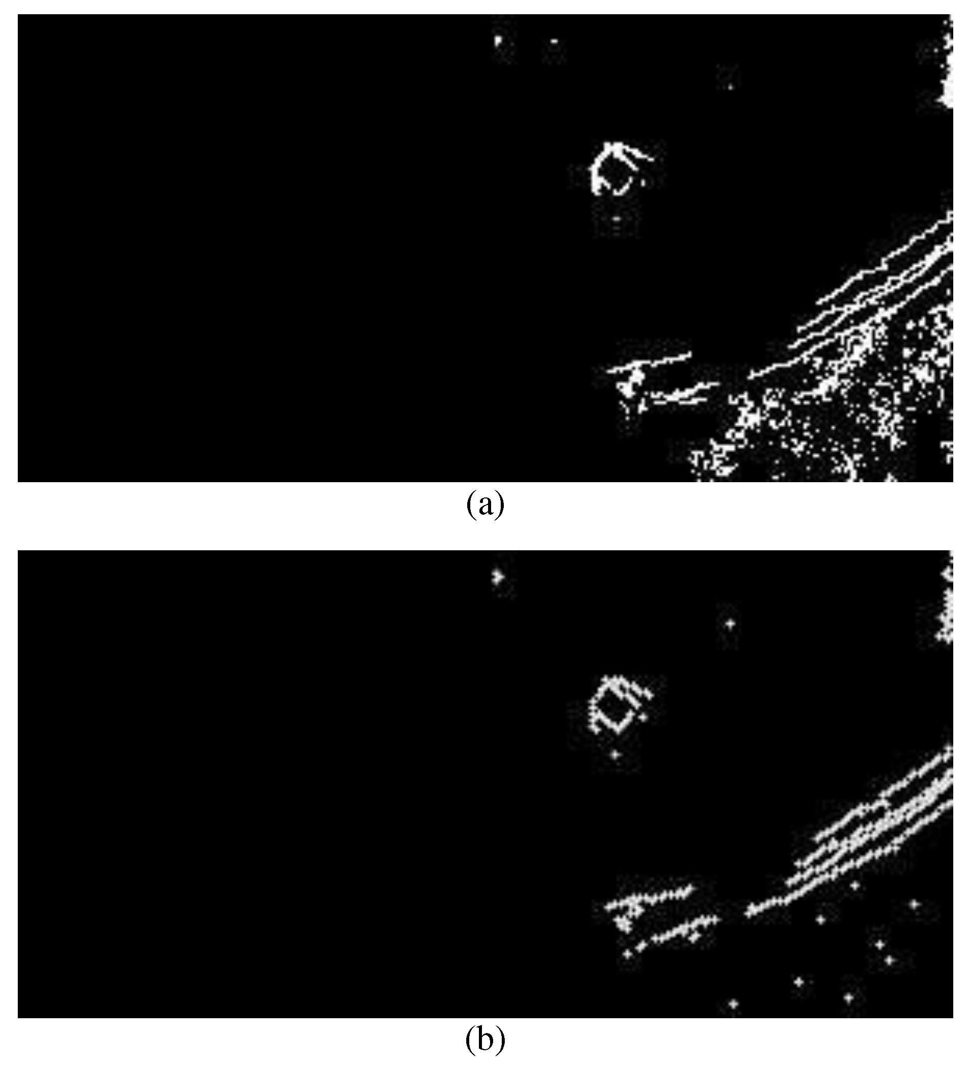
Figure 17.
Obstacle detection results comparison chart: (a) Rectangle box size. (b) Rectangle box size.
Figure 17.
Obstacle detection results comparison chart: (a) Rectangle box size. (b) Rectangle box size.
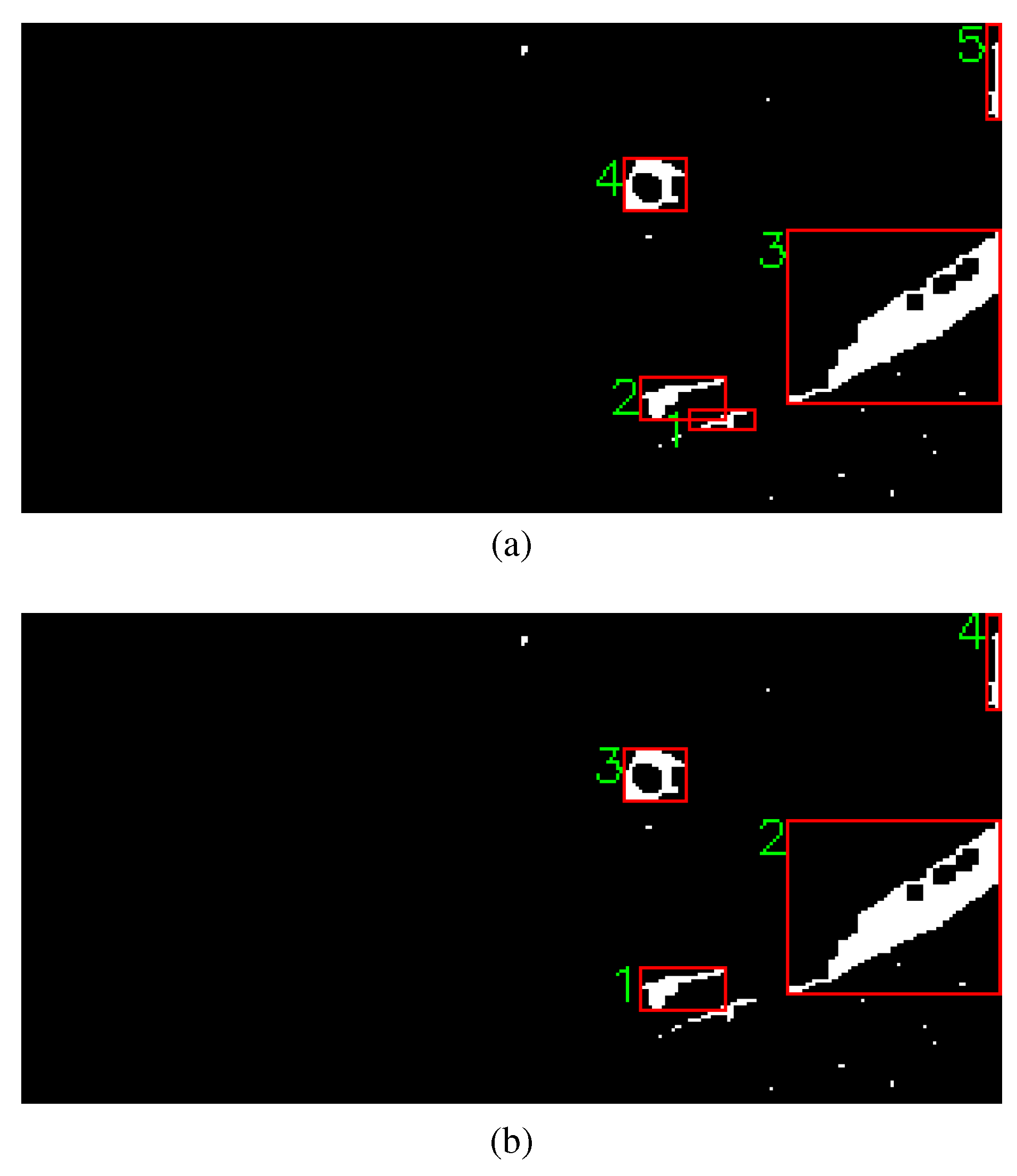

Table 1.
Variable Symbols.
| Direction | x-Axial | y-Axial | z-Axial |
|---|---|---|---|
| Velocity | u | v | w |
| Rotation angle | |||
| Angular velocity | p | q | r |
| Forces | X | Y | Z |
| Torque | K | M | N |
Table 2.
Unmanned catamaran parameters.
| Symbol | Description | Value/Unit |
|---|---|---|
| m | Unmanned vessel mass | 67.40 kg |
| L | Length | 1.235 m |
| B | Width | 0.956 m |
| d | Full load draft | 0.168 m |
| Thruster to the center distance | 0.34 m |
Table 3.
Fuzzy rule table of fuzzy adaptive PID control algorithm
| e | |||||||
|---|---|---|---|---|---|---|---|
| ec | NB | NM | NS | Z | PS | PM | PB |
| NB | PB | PB | PM | PM | PS | Z | Z |
| NM | PB | PB | PM | PS | PS | Z | NS |
| NS | PM | PM | PM | PS | Z | NS | NS |
| Z | PM | PM | PS | Z | NS | NM | NM |
| PS | PS | PS | Z | NS | NS | NM | NM |
| PM | PS | Z | NS | NM | NM | NM | NB |
| PB | Z | Z | NM | NM | NM | NB | NB |
Table 4.
Fuzzy rule table of fuzzy adaptive PID control algorithm
| e | |||||||
|---|---|---|---|---|---|---|---|
| ec | NB | NM | NS | Z | PS | PM | PB |
| NB | NB | NB | NM | NM | NS | Z | Z |
| NM | NB | NB | NM | NS | NS | Z | Z |
| NS | NB | PM | NS | NS | Z | PS | PS |
| Z | NM | NM | NS | Z | PS | PM | PM |
| PS | NM | NS | Z | PS | PS | PM | PB |
| PM | Z | Z | PS | PS | PM | PB | PB |
| PB | Z | Z | PM | PM | PM | PB | PB |
Table 5.
Fuzzy rule table of fuzzy adaptive PID control algorithm
| e | |||||||
|---|---|---|---|---|---|---|---|
| ec | NB | NM | NS | Z | PS | PM | PB |
| NB | PS | NS | NB | NB | NB | NM | PS |
| NM | PS | NS | NB | NM | NM | NS | Z |
| NS | Z | NS | NM | NM | NS | NS | Z |
| Z | Z | NS | NS | NS | NS | NS | Z |
| PS | Z | Z | Z | Z | Z | Z | Z |
| PM | PB | NS | PS | PS | PS | PS | PB |
| PB | PB | PM | PM | PM | PS | PS | PB |
Table 6.
Track points to be tracked
| Point No. | Latitude | Longitude |
|---|---|---|
| 1 | 30°46’21.6403" | 104°58’48.6782" |
| 2 | 30°46’20.9004" | 104°58’48.4626" |
| 3 | 30°46’20.9601" | 104°58’48.1879" |
| 4 | 30°46’21.8029" | 104°58’48.3499" |
| 5 | 30°46’21.8427" | 104°58’48.1684" |
| 6 | 30°46’21.0995" | 104°58’47.9035" |
| 7 | 30°46’21.2156" | 104°58’47.7418" |
| 8 | 30°46’22.0319" | 104°58’47.9819" |
Disclaimer/Publisher’s Note: The statements, opinions and data contained in all publications are solely those of the individual author(s) and contributor(s) and not of MDPI and/or the editor(s). MDPI and/or the editor(s) disclaim responsibility for any injury to people or property resulting from any ideas, methods, instructions or products referred to in the content. |
© 2023 by the authors. Licensee MDPI, Basel, Switzerland. This article is an open access article distributed under the terms and conditions of the Creative Commons Attribution (CC BY) license (http://creativecommons.org/licenses/by/4.0/).
Copyright: This open access article is published under a Creative Commons CC BY 4.0 license, which permit the free download, distribution, and reuse, provided that the author and preprint are cited in any reuse.


