Algorithm Optimizer in GA-LSTM for Stock Price Forecasting

1. Introduction

Public investment awareness is increasing and investment instruments that are currently quite attractive to the public are stocks. It is impossible to know for sure what the future will be like. The existence of supply and demand for shares in the capital market makes stock prices fluctuate[1] which can make it difficult for investors to see investment opportunities in a company's shares. One tool that can help investors overcome this is forecasting techniques [2]. Time series forecasting represents many real challenges, such as stock price forecasting, language processing, or weather forecasting that directly or indirectly affects human life [3].

Time series data that is available in large quantities can be converted into information that will be used for forecasting [4]. Forecasting is used to predict what might happen in the future[5]. The process of data forecasting can be simplified and accelerated with the help of the latest breakthroughs in computer technology. In artificial intelligence, time series data is just one area where machine learning has significantly improved. It can be said that deep learning uses artificial neural networks because it is a machine learning technique that mimics the neural network architecture of the human brain. According to [6] Artificial Neural Networks (ANN) are connectionist agent networks that study and transmit information from one artificial neuron to another, taking inspiration from biological neurons. According to [7] ANN was found to be a useful model as an information manager that has a similar function to the biological nervous system of the human brain that can be applied to problem-solving. Deep representation learning, often known as Deep Learning (DL), is the process of studying a hierarchy of representations or characteristics as inputs move between neurons. The DL approach learns the input to produce higher performance accuracy [8].

The time series data technique is made for nonlinear data because it contains dynamic data and data with broad dimensions. The type of deep learning based on nonlinear predictions is a recurrent neural network [9]. One of the deep learning that can work for time series is the Recurrent Neural Network (RNN), which is designed to work with sequential data [10] [11]. The progress of RNN is growing quite rapidly in various fields, but RNN has a weakness in processing time series because, [12] performance for prediction will have a negative effect if the sequence size is relevantly long and the other is that the RNN gradient will be lost, resulting in long-term memory failure. Hochreiter et al. created LSTM as a floating RNN to deal with these weaknesses [13]. Deep learning’s training and success are strongly influenced by the selection of hyperparameters. Hyperparameters are the variables whose values ​​are manually assigned to the model to assist in learning [14]. Research conducted by [15] succeeded in finding hyperparameters through the implementation of a Genetic Algorithm - Long Short-Term Memory in finding the best model. GA, a heuristic search and optimization technique that imitates the evaluation process [16] Optimization itself is a process of solving certain problems in order to be in the most favorable condition [17]. GA is widely used to find optimal approximation solutions for optimization problems with large search space. This research uses a hybrid method between the Genetic Algorithm and Long Short-Term Memory to find a suitable model for predicting stock prices. Genetic Algorithm is used in optimizing the architecture such as the number of epochs, window size, and the number of LSTM units in the hidden layer. The selection of the right algorithm optimizaters will produce the best value for each parameter model. Because optimizer are a way to achieve the best value [18], therefore, an optimization setting will also be carried out using several optimizers to get the best value.

In his research [19], the authors extract historical monthly financial time data from January 1985 to August 2018 from the Yahoo Finance website. The Nikkei 225 index (N225), the NASDAQ composite index (IXIC), the Hang Seng Index (HIS), the S&P 500 commodity prices index (GSPC), and the Dow Jones industrial average index are all included in the monthly statistics (DJ). In addition, the authors compile monthly economic time series for various periods from the websites of the International Monetary Fund (IMF) and the Federal Reserve Bank of St. Louis. Housing for all urban consumers, Index 1982-1984=100 for the period January 1967 to July. 2017 (MC), Commodity of medical care for all urban consumers, Index 1982-1984=100 for the period January 1967 to July 2017 (HO), trade-weighted US dollar index expressed in major currencies, Mar Index 1973=100 for the period August 1967 to July 2017 (EX), Food and Beverages for all Urban Consumers, Index 1982-1984=100 for the period January 1967 to July 2017 (FB), M1 Stock Money, billions of rupiah for the period January 1959 to July 2017 (MS), and Transportation for All Urban Consumers, Index 1982-1984=100 for the period January 1947 to July 2017 (TR). The following variables are included in each financial time series data set: Open, High, Low, Close, Adjusted Close, and Volume. The only component of the financial time series that I include in the ARIMA and LSTM models is the "Adjusted Close" variable. In assessing the effectiveness of two techniques for forecasting time series data, namely LSTM and ARIMA, these two strategies were used together with a set of financial data, and the results showed that LSTM outperformed ARIMA. The LSTM-based algorithm specifically improves predictions by 85% on average more than ARIMA.

[20] using the LSTM-RNN method with historical stock data of AAPL (Apple Inc.), GOOG (Google) and TSLA (Tesla, Inc.) with Adam optimization. Regression, Support Vector Machine, Random Forest, Feed Forward Neural Network, and Backpropagation are some examples of traditional machine learning algorithms that have been used to compare models. The findings show that when compared to conventional machine learning methods, the RNN-LSTM model tends to give more accurate results.

[21] uses the Long Short-Term Memory (LSTM) approach to predict the time series Bank BRI shares, with the selection of 9 epochs resulting in an RMSE of 227, 470333244533 which is considered quite good and visually shows a prediction graph that is almost identical to the original data.

Research conducted by [22] on the use of two secondary data, namely stock index data and the USD to IDR exchange rate to make stock price forecasts in Indonesia using from 09 June 2019 to 06 June 2019 with the LSTM method which produces testing under LSTM can predict stock prices from 2017 to 2019 well, shown through the results of error, so that conclusions can be drawn with accurate results, LSTM can estimate stock prices and can overcome long-term dependencies.

The research conducted by [23] on the implementation of LSTM on stock prices of three plantation companies in Indonesia resulted in the best LSTM for SSMS shares was 70, which resulted in RMSE 21,328 using hidden neurons and the RMSProp optimizer option. Then, the best LSTM model is the stock LSIP, which results in an RMSE score of 33,097 with Adam and hidden neurons set to a maximum of 80 in the optimizer. The best model is the SIMP stock, which when used with the Adamax optimizer setting and 100 hidden neurons, results in an RMSE score of 8.337.

Research conducted by [17] on the optimization of artificial neural networks with genetic algorithms used to predict credit card approval by applying the neural network obtained an increase in results from 85.42% to 87.82%. Then there is a study conducted by [15] in predicting KOSPI stock prices by applying the use of Genetic Algorithm - Long Short-Term Memory to produce the best LSTM model by setting a window size 10 and compiling 2 hidden layers with nodes of 15 and 7 respectively, the MSE and MAE were 181.99% and 10.21%, respectively.

2. Materials and Methods

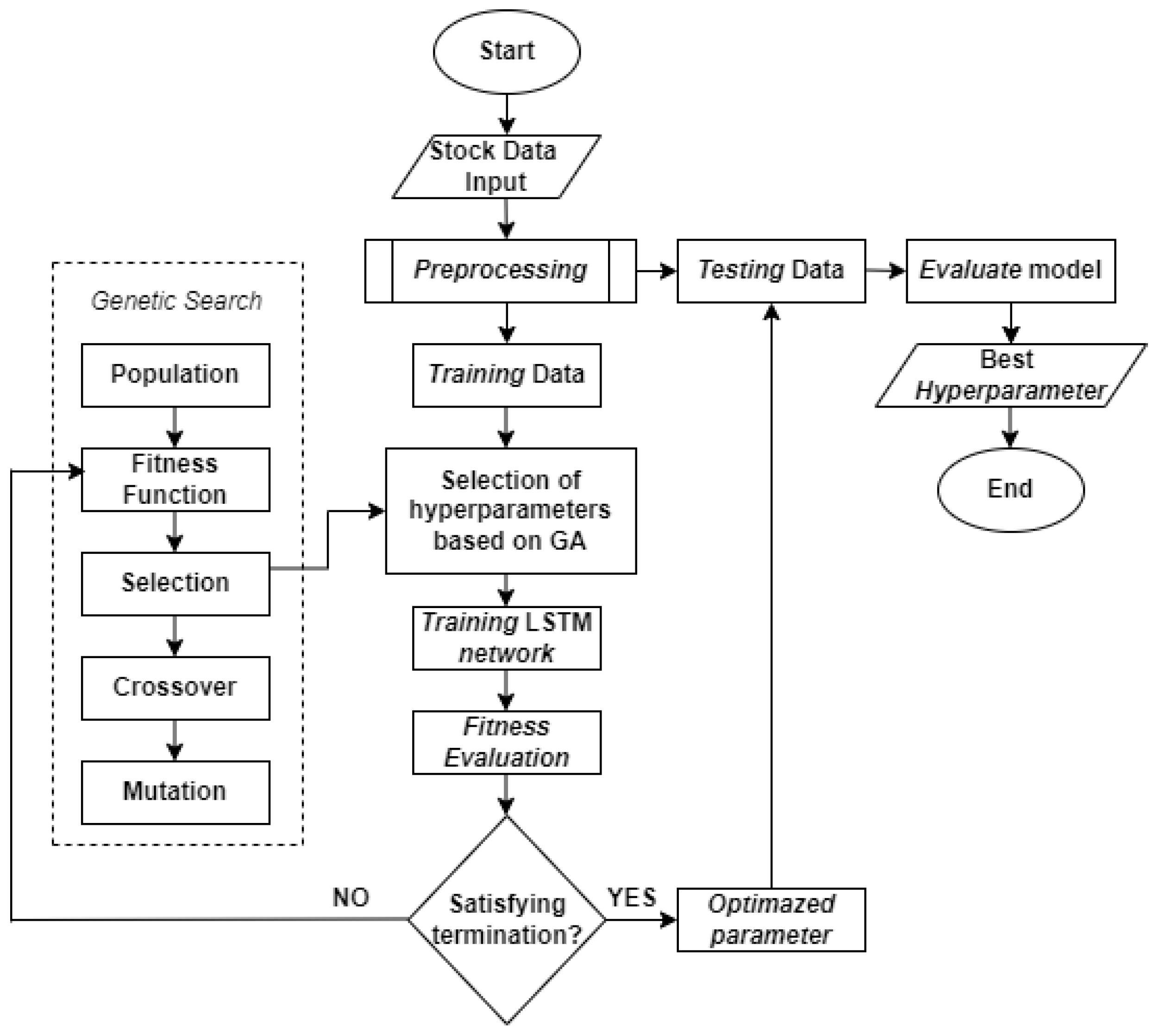
In this study, the Genetic Algorithm – Long Short-Term Memory (GA-LSTM) method is applied for forecasting the stock price of PT Bank Rakyat Indonesia (Persero) Tbk and PT Bank Mandiri (Persero) Tbk. The data collected and used in this study is the stock price dataset of Bank BRI [24] and Bank Mandiri [25] which was taken on February 3, 2022 in the form of CSV (Comma Separated Values) format obtained from the website www.finance.yahoo.com. The data used is close price as much as 2,487 price data which is converted into a format that can be used python using the Pandas module.

It is then checked whether there is missing or incomplete data, so that the missing data does not affect the overall data processing. Then, it is necessary to transform the data and normalize the data before using it. The data transformation is carried out to make the data stationary where the data to be used does not have a tendency to a certain trend. For the normalization in this study, we use the implementation of the transformation object from the -learn class scikit. Furthermore, the data is divided into training and the remaining 20% data for testing data. This study uses an LSTM design with 3 neural and a Dropout module for each layer, uses a loss function mean squared error and uses several optimizers with the TensorFlow library.

LSTM has four components, namely input gate, forget gate, cell state, and output gate [26]. Input gate has two functions; to receive new information: $rt$ and dt .rt prearranging hidden vectors $h_{t-1}$ with new information $x_t$. That is, $[h_{t-1}, x_t]$, then multiplied by the weight matrix $W_r$, after that plus the noise vector $b_r$ . $Dt$ does the same. Then multiply $rt$and $dt$by element -wise to get the cell state $ct$.

$$r_t=\sigma (W_r.\left[h_{t-1},x_t\right]+b_r)$$

(1)

$$d_t=tanh(W_d.\left[h_{t-1},x_t\right]+b_d)$$

(2)

Forget gate f t looks like that similar to rt in input gate. This gate controls the limit until the value is stored in memory.

$$f_t=\sigma (W_f.\left[h_{t-1},x_t\right]+b_f)$$

(3)

Cell state is used for multiplication calculation based on the element between the previous cell state 𝐶_{𝑡−1 ,} and forget gate ft then added the result of input gate rt and dt.

$$C_t=f_t.C_{t-1}+r_t.d_t$$

(4)

Here, $o_t$ is output gate in time $t$, and $W_o$ and $b_o$ is weights line and bias for gate output . $H_t$ is hidden layer will go to in the next step, or up to output as applying $y_t$ obtained by tanh to $h_t$_.Note that the output $o_t$is not the output of $y_t$ , but the gate the used to control the output.

$$o_t=\sigma (W_o.\left[h_{t-1},x_t\right]+b_o)$$

(5)

$$h_t=o_{t}tanh C_t$$

(6)

In their book, [27] argues optimizer that is most widely used in deep learning is the mini-batch consisting of Adagrad, Adadelta, RMSprop, Nadam, and Adam.

In Adagrad deployments, the learning rate is normalized for each dimension on which the cost function depends. The learning rate in each iteration is the learning rate divided by the norm $l2$ of the gradient the previous to the current iteration for each dimension. The formula used in Adagrad is as follows:

$$S_t=S_{t-1}+{\left[\frac{\partial L}{\delta wt}\right]}^2$$

(7)

$$w_{t+1}=w_t-\frac{\alpha }{\sqrt{S_t+ϵ}} . \frac{\partial L}{\delta w_t}$$

(8)

Description:

$t$ = for time step

$w$ = weight/ parameter to be updated

$\alpha$ = learning rate (0.001)

$\frac{\partial L}{\delta w}$ = gradient L (Loss function)

S = cumulative sum of squares of gradient current and

Previous is an Adagrad extension as an alternative to reduce Adagrad's aggressiveness, reduce learning rate monotonically, also focus more on the learning rate. The formula used is as follows:

$$D_t= \beta D_{t-1}+\left(1-\beta \right){\left[∆w_t\right]}^2$$

(9)

$$S_t=\beta S_{t-1}+(1-\beta ){\left[\frac{\partial L}{\partial wt}\right]}^2$$

(10)

$$w_{t+1}=w_t-\frac{\sqrt{D_{t-1}+ϵ}}{\sqrt{S_t+ϵ}} . \frac{\partial L}{\partial w_t}$$

(11)

Description:

D = difference between the current weight and the updated weight

$\beta$ = 0.9

$ϵ$ = 1e-7

RMSprop is learning rate which is an improvement on Adagrad. The formula used is as follows:

$$S_t= \beta S_{t-1}+(1-\beta ){\left[\frac{\partial L}{\partial wt}\right]}^2$$

(12)

$$w_{t+1}=w_t-\frac{\alpha }{\sqrt{S_t+ϵ}} . \frac{\partial L}{\partial w_t}$$

(13)

RMSprop and AdaGrad are combined with momentum to form Adam. Adam measures learning rates via a quadratic gradient, similar to RMSprop, and uses dynamic gradient averaging to take advantage of momentum [26]. The formula used is as follows:

$${\widehat{V}}_t=\frac{V_t}{1-{\beta }_1^t}$$

(14)

$${\widehat{S}}_t=\frac{S_t}{1-{\beta }_2^t}$$

(15)

$$w_{t+1}=w_t-\frac{\alpha }{\sqrt{{\widehat{S}}_t+\in }} . {\widehat{V}}_t$$

(16)

Description:

$\widehat{V}$ = average gradient with momentum replacing gradient current

$\widehat{S}$ = average cumulative sum of squares of gradients current and previous

${\beta }_1$ = 0.9

${\beta }_2$ = 0.999

$ϵ$ = 1e-7

Nadam is used for noisy gradient or gradient with high curvature. The learning process is accelerated by adding up the decay of the moving average for the previous and current gradients, Nadam takes gradients one step further by using Nestrove to replace $\widehat{V}$ in the previous equation with $\widehat{V.}$ the currentThe formula used is as follows:

$$w_{t+1}=w_t-\frac{\alpha }{\sqrt{{\widehat{S}}_t+\in }}\left({\beta }_1{\widehat{V}}_t+\frac{{1-\beta }_1}{1-{\beta }_1^t} . \frac{\partial L}{\partial w_t}\right)$$

(17)

where,

$${\widehat{V}}_t=\frac{V_t}{1-{\beta }_1^t} ; {\widehat{S}}_t=\frac{S_t}{1-{\beta }_2^t}$$

(18)

Description:

$\alpha$ = learning rate (0.002)

${\beta }_1$ = 0.9

${\beta }_2$ = 0.999

$ϵ$ = 1e-7

While for the initialization design of the Genetic-Algorithm using DEAP library from python, the initial stage is carried out by determining the initial population which is a collection of chromosomes containing solutions for the number of window sizes, epochs, and the number of units. The formation of chromosomes is done in binary using binary numbers. The basic structure of the genetic algorithm consists of several steps [28], namely: 1) Initialization of the population; 2) Population evaluation; 3) Selection of the population to be subjected to genetic operators; 4) The process of crossover of certain chromosome pairs; 5) Certain chromosomal mutation processes; 6) Evaluation of the new population; 7) Repeat from Step 3 if the stop condition is not met. In this study using: population = 5, maximum generation = 10, crossover rate = 0.4 and mutation rate = 0.1. Each design is carried out to evaluate the suitability of the GA. The GA process is repeated more than once by setting different values ​​for the number of window sizes, epochs, and number of units.

Figure 1. GA-LSTM model flowchart.

Figure 1. GA-LSTM model flowchart.

3. Results and Discussion

The research uses the GA-LSTM method as a calculation process by applying several different optimizations to find hyperparameters of the number of epochs, window sizes, and the number of LSTM units in the hidden layer. In this study, it is limited to using close for this type of prediction price. The results of this study are the model with the hyperparameters obtained from training and testing data with the lowest MAE and MAPE values, then the obtained model can be used to predict the stock’s price.

Root Mean Square Error (RMSE) is used to measure the difference between the estimated target and the actual target by calculating the square root value of the MSE. The higher the value produced by the RMSE, the lower the level of accuracy, and vice versa, if the value of the resulting RMSE is lower, the level of accuracy is higher [29]. The RMSE formula is shown in the following equation.

$$RMSE=\sqrt{\sum _{i=1}^n\frac{{\left({\widehat{y}}_i-y_{i }\right)}^2}{n}}$$

(20)

Description:

$y_i$ = value of the i

${\widehat{y}}_i$ = result forecast

$n$ = amount of data

Mean Absolute Percentage Error (MAPE) to measure error by calculating the average method the average absolute error divided by the true value, which results show the absolute percentage error value of the predicted model results. The prediction model is getting better if the MAPE value is lower [30]. The RMSE formula is shown in the following equation.

$$MAPE=\frac{100\%}{n}\sum \left|\frac{y-\widehat{y}}{y}\right|$$

(21)

Description:

$\widehat{y}$ = value of forecast results

$y$ = value of observation to -i

$n$ = amount of data

Table 1. Range MAPE value [31].

Range MAPE	Meaning
<10%	Accuracy rate is very good
10 – 20%	Accuracy rate is good
20 – 50%	Accuracy rate is decent
>50%	Accuracy rate bad

Table 1. Range MAPE value [31].

Range MAPE	Meaning
<10%	Accuracy rate is very good
10 – 20%	Accuracy rate is good
20 – 50%	Accuracy rate is decent
>50%	Accuracy rate bad

After doing all stages of the research, the output is in the form of RMSE and MAPE values, as well as a graph of the comparison of the original price with the predicted data, the results are shown as follows.

Case-1 Shares of Bank BRI

Table 2. Forecasting results with Adagrad optimizer.

Epochs	Neurons	Window Size	Data	RMSE	MAPE(%)
33	[4, 4, 3]	1	Training	100.58	1.49
			Testing	94.43	1.86
38	[4, 4, 3]	1	Training	108.31	1.53
			Testing	95.39	1.88

Table 2. Forecasting results with Adagrad optimizer.

Epochs	Neurons	Window Size	Data	RMSE	MAPE(%)
33	[4, 4, 3]	1	Training	100.58	1.49
			Testing	94.43	1.86
38	[4, 4, 3]	1	Training	108.31	1.53
			Testing	95.39	1.88

In the model using Adagrad optimizer with hyperparameter, the number of epochs is 33, window size is1, and the number of LSTM units in the hidden layer are [4, 4, 3], the RMSE and MAPE values ​​during training are 100.58 and 1.49%, while in testing are 94.43 and 1.86%. Then the model with hyperparameter number epochs is 38, window size is 1, and the number of LSTM units in the hidden layer is [4, 4, 3], the RMSE and MAPE values ​​during training are 108.30 and 1.53%, while in testing namely 95.39 and 1.88%.

Table 3. Forecasting results with Adadelta optimizer.

Epochs	Neurons	Window Size	Data	RMSE	MAPE(%)
35	[1, 3, 2]	1	Training	106.43	1.51
			Testing	94.47	1.86
18	[2, 1, 4]	2	Training	99.69	1.58
			Testing	98.09	1.91

Table 3. Forecasting results with Adadelta optimizer.

Epochs	Neurons	Window Size	Data	RMSE	MAPE(%)
35	[1, 3, 2]	1	Training	106.43	1.51
			Testing	94.47	1.86
18	[2, 1, 4]	2	Training	99.69	1.58
			Testing	98.09	1.91

In the model using Adadelta optimizer with hyperparameter, the number of epochs is 35, window size is 1, and the number of LSTM units in the hidden layer are [1, 3, 2], RMSE and MAPE values ​​during training namely 106.43 and 1.51%, while in testing it is 94.47 and 1.86%. Then the model with hyperparameter number epochs is 18, window size is 2, and the number of LSTM units in the hidden layer is [2, 1, 4], the RMSE and MAPE values ​​during training are 99, 69 and 1.58%, while in testing namely 98.09 and 1.91%.

Table 4. Forecasting results with RMSprop optimizer.

Epochs	Neurons	Window Size	Data	RMSE	MAPE(%)
41	[4, 5, 5]	1	Training	102.91	1.52
			Testing	94.40	1.88
43	[3, 1, 4]	5	Training	102.83	1.53
			Testing	95.49	1.91

Table 4. Forecasting results with RMSprop optimizer.

Epochs	Neurons	Window Size	Data	RMSE	MAPE(%)
41	[4, 5, 5]	1	Training	102.91	1.52
			Testing	94.40	1.88
43	[3, 1, 4]	5	Training	102.83	1.53
			Testing	95.49	1.91

In the model that uses RMSprop optimizer with hyperparameter, the number of epochs is 41, window size is 1, and the number of LSTM units is hidden layers are [4, 5, 5], the RMSE and MAPE values ​​during training are 102.91 and 1.52%, while in testing are 94.40 and 1.88%. Then the model with hyperparameter number epochs is 43, window size is 5, and the number of LSTM units in the hidden layer is [3, 1, 4], the RMSE and MAPE values ​​during training are 102.83 and 1.53%, while in testing namely 95.49 and 1.91%.

Table 5. Forecasting results with Adam optimizer.

Epochs	Neurons	Window Size	Data	RMSE	MAPE(%)
38	[4, 5, 2]	4	Training	94.28	1.51
			Testing	95.49	1.87
24	[4, 5, 2]	2	Training	95.93	1.51
			Testing	95.06	1.87

Table 5. Forecasting results with Adam optimizer.

Epochs	Neurons	Window Size	Data	RMSE	MAPE(%)
38	[4, 5, 2]	4	Training	94.28	1.51
			Testing	95.49	1.87
24	[4, 5, 2]	2	Training	95.93	1.51
			Testing	95.06	1.87

In the model using Adam optimizer with hyperparameter, the number of epochs is 38, window size is 4, and the number of LSTM units is hidden layers are [4, 5, 2], the RMSE and MAPE values ​​during training are 94.28 and 1.51%, while in testing are 95.49 and 1.87%. Then the model with hyperparameter number epochs is 24, window size is 4, and the number of LSTM units in the hidden layer is [4, 5, 2], the RMSE and MAPE values ​​during training are 95.93 and 1.51%, while in testing namely 95.06 and 1.87%.

Table 6. Forecasting results using Nadam optimizer.

Epochs	Neurons	Window Size	Data	RMSE	MAPE(%)
15	[3, 3, 2]	6	Training	93.03	1.51
			Testing	95.62	1.87
28	[4, 5, 4]	2	Training	95.99	1.50
			Testing	95.17	1.87

Table 6. Forecasting results using Nadam optimizer.

Epochs	Neurons	Window Size	Data	RMSE	MAPE(%)
15	[3, 3, 2]	6	Training	93.03	1.51
			Testing	95.62	1.87
28	[4, 5, 4]	2	Training	95.99	1.50
			Testing	95.17	1.87

In the model using Nadam optimizer with hyperparameters, the number of epochs is 15, window size is 6, and the number of LSTM units is hidden layers are [3, 3, 2], the RMSE and MAPE values ​​during training are 93.03 and 1.51%, while in testing are 95.62 and 1.87%. Then the model with hyperparameter number epochs is 28, window size is 2, and the number of LSTM units in the hidden layer is [4, 5, 4], the RMSE and MAPE values ​​during training are 95.99 and 1.51%, while in testing namely 95.17 and 1.87%.

Case-2 Shares of Bank Mandiri

Table 7. Forecasting results with Adagrad optimizer.

Epochs	Neurons	Window Size	Data	RMSE	MAPE(%)
36	[1, 5, 1]	​​4	Training	105.87	1.37
			Testing	153.16	1.89
14	[4, 3, 2]	5	Training	109.39	1.42
			Testing	152.89	1.92

Table 7. Forecasting results with Adagrad optimizer.

Epochs	Neurons	Window Size	Data	RMSE	MAPE(%)
36	[1, 5, 1]	​​4	Training	105.87	1.37
			Testing	153.16	1.89
14	[4, 3, 2]	5	Training	109.39	1.42
			Testing	152.89	1.92

In the model using Adagrad optimizer with hyperparameter, the number epochs is 36, window size is 4, and the number of LSTM units in the hidden layer are [1, 5, 1], the RMSE and MAPE values ​​during training are 105.87 and 1.37%, while in testing are 153.16 and 1.89%. Then the model with hyperparameter number epochs is 14, window size is 5, and the number of LSTM units in the hidden layer is [4, 3, 2], the RMSE and MAPE values ​​during training are 109.39 and 1.42%, while in testing namely 152.89 and 1.92%.

Table 8. Forecasting results with Adadelta optimizer.

Epochs	Neurons	Window Size	Data	RMSE	MAPE(%)
35	[3, 5, 4]	3	Training	108.21	1.43
			Testing	152.84	1.94
30	[5, 2, 5]	6	Training	110.35	1.45
			Testing	153.51	1.93

Table 8. Forecasting results with Adadelta optimizer.

Epochs	Neurons	Window Size	Data	RMSE	MAPE(%)
35	[3, 5, 4]	3	Training	108.21	1.43
			Testing	152.84	1.94
30	[5, 2, 5]	6	Training	110.35	1.45
			Testing	153.51	1.93

In the model that uses Adadelta optimizer with hyperparameter, the number of epochs is 35, window size is 3, and the number of LSTM units in the hidden layer are [3, 5, 4], the RMSE and MAPE values ​​during training namely 1068.21 and 1.43%, while in testing it is 152.84 and 1.94%. Then the model with hyperparameter number epochs is 30, window size is 6, and the number of LSTM units in the hidden layer is [5, 2, 5], the RMSE and MAPE values ​​during training are 110.35 and 1.45%, while in testing namely 153.51 and 1.93%.

Table 9. Forecasting results with RMSprop optimizer.

Epochs	Neurons	Window Size	Data	RMSE	MAPE(%)
20	[2, 2, 2]	2	Training	104.99	1.35
			Testing	150.06	1.88
20	[3, 3, 5]	5	Training	105.00	1.35
			Testing	151.44	1.89

Table 9. Forecasting results with RMSprop optimizer.

Epochs	Neurons	Window Size	Data	RMSE	MAPE(%)
20	[2, 2, 2]	2	Training	104.99	1.35
			Testing	150.06	1.88
20	[3, 3, 5]	5	Training	105.00	1.35
			Testing	151.44	1.89

In the model that uses RMSprop optimizer with hyperparameter, the number of epochs is 20, window size is 2, and the number of LSTM units is hidden layers are [2, 2, 2], the RMSE and MAPE values ​​during training are 104.99 and 1.35%, while in testing are 150.06 and 1.88%. Then the model with hyperparameter number epochs is 20, window size is 5, and the number of LSTM units in the hidden layer is [3, 3, 5], the RMSE and MAPE values ​​during training are 105.00 and 1.35%, while in testing namely 151.44 and 1.89%.

Table 10. Forecasting results with Adam optimizer.

Epochs	Neurons	Window Size	Data	RMSE	MAPE(%)
15	[5, 1, 4]	3	Training	105.15	1.35
			Testing	150.37	1.88
25	[3, 3, 2]	5	Training	105.10	1.35
			Testing	150,41	1.88

Table 10. Forecasting results with Adam optimizer.

Epochs	Neurons	Window Size	Data	RMSE	MAPE(%)
15	[5, 1, 4]	3	Training	105.15	1.35
			Testing	150.37	1.88
25	[3, 3, 2]	5	Training	105.10	1.35
			Testing	150,41	1.88

In the model using Adam optimizer with hyperparameter, the number of epochs is 15, window size is 3 and the number of LSTM units in the hidden layer namely [5, 1, 4], the RMSE and MAPE values ​​during training were 105.15 and 1.35%, while in testing were 150.37 and 1.88%. Then the model with hyperparameter number epochs is 25, window size is 5, and the number of LSTM units in the hidden layer is [3, 3, 2], the RMSE and MAPE values ​​during training are 105.10 and 1.35%, while in testing namely 150.41 and 1.88%.

Table 11. Forecasting results with Nadam optimizer.

Epochs	Neurons	Window Size	Data	RMSE	MAPE(%)
44	[3, 5, 3]	5	Training	105.05	1.35
			Testing	151.59	1.89
21	[4, 3, 5]	6	Training	105.02	1.35
			Testing	150,91	1,89

Table 11. Forecasting results with Nadam optimizer.

Epochs	Neurons	Window Size	Data	RMSE	MAPE(%)
44	[3, 5, 3]	5	Training	105.05	1.35
			Testing	151.59	1.89
21	[4, 3, 5]	6	Training	105.02	1.35
			Testing	150,91	1,89

In the model using Nadam optimizer with hyperparameters, the number of epochs is 44, window size is 5, and the number of LSTM units is hidden layers are [3, 5, 3], the RMSE and MAPE values ​​during training are 105.05 and 1.35%, while in testing are 151.59 and 1.89%. Then the model with hyperparameter number epochs is 21, window size is 6, and the number of LSTM units in the hidden layer is [4, 3, 5], the RMSE and MAPE values ​​during training are 105.02 and 1.35%, while in testing namely 150.91 and 1.89%.

From the results of training and testing of each optimization with a different case, it can be seen that the resulting RMSE value shows a small value, which means that the model generated from this prediction has a small error rate. And the results of the MAPE value have a value below 10% which shows the prediction model has a very good level of accuracy. With the results of using several optimizations to produce small RMSE and MAPE values, in this study it can be said that GA-LSTM can improve performance and save time. Therefore, in one process we can find hyperparameters to use. Even so, if you look at tables 2 to 6, it can be seen that the MAPE values ​​generated by the optimizers Adam and Nadam have the same value. In the RMSE in Adam's first model between training and testing difference error of 1.21 and in the second model it has an error 0.87. While the RMSE in the first model of Nadam between training and testing difference error of 2.56 and in the second model it has an error 0.82. Then from table 7 to table 8 it can be seen that the MAPE value generated by the two models by optimizers has the same value. Therefore, it seems that the value is quite stable and small using the Adam optimizer.

4. Conclusion

The application of the Genetic Algorithm – Long Short-Term Memory shows very good results, as evidenced by the RMSE and MAPE values ​​generated in the training and testing of data which show a fairly low error rate and a fairly good level of accuracy with MAPE value below 10% in every optimizer used. The error rate generated is quite low, in case-1 with a minimum RMSE value of 93.03 and 94.40 and in case-2 with an RMSE value of 104.99 and 150.06 during training and testing. A fairly stable and small value is generated by the setting using the Adam optimizer. The next research can be used to look for the other hyperparameters or can apply hybrid Algorithm with other deep learning methods. This research is expected to be applied on the same data’s characteristics using Genetic Algorithm—Long Short-Term Memory to look for the hyperparameter.

References

- B. D. Prasetya, F. S. Pamungkas, and I. Kharisudin, Stock Data Modeling and Forecasting with Time Series Analysis using Python, Prism. Pros. Semin. Nas. Mat., pp. 714–718. 2019.
- P. Jadmiko, Forecasting Of Stock Prices On Indonesian Sharia Stock Index (Issi) Using Fuzzy Time Series Markov Chain, FMIPA, Universitas Islam Indonesia, Yogyakarta, 2018.
- J. K. Lubis and I. Kharisudin, Long Short Term Memory Method and Generalized Autoregressive Conditional Heteroscedasticity for Stock Data Modeling, Prism. Pros. Semin. Nas. Mat., pp. 652–658, 2021.
- N. Mishra, H. K. Soni, S. Sharma, and A. K. Upadhyay, A comprehensive survey of data mining techniques on time series data for rainfall prediction, J. ICT Res. Appl., 11(2), pp. 167–183, May. 2017. [CrossRef]
- D. Ayu Rezaldi, ARIMA Method Forecasting Stock Data PT. Indonesian Telecommunications, Prism. Pros. Semin. Nas. Mat., pp. 611–620, 2021.
- E. Bisong, Building Machine Learning and Deep Learning Models on Google Cloud Platform: A Comprehensive Guide for Beginners, Apress Media LLC. 2019. [CrossRef]
- O. I. Abiodun, A. Jantan, A. E. Omolara, K. V. Dada, N. A. E. Mohamed, and H. Arshad, State-of-the-art in artificial neural network applications: A survey, Heliyon, 4(11), p. 1-41, November. 2018. [CrossRef]
- L. R. Varghese and V. Kandasamy, Convolution and recurrent hybrid neural network for hevea yield prediction, J. ICT Res. Appl., (15)2, pp. 188–203, August. 2021. [CrossRef]
- K. Chen, Y. Zhou, and F. Dai, A LSTM-based method for stock returns prediction: A case study of China stock market, Proc. 2015 IEEE Int. Conf. Big Data (Big Data) 2015, pp. 2823–2824, 2015.
- Z. C. Lipton, J. Berkowitz, and C. Elkan, A Critical Review of Recurrent Neural Networks for Sequence Learning, arXiv preprint arXiv, pp. 1–38, Oct. 2015.
- Z. Hu, Y. Zhao, and M. Khushi, A survey of forex and stock price prediction using deep learning, Appl. Syst. Innov., (4)1, pp. 1–30, February. 2021. [CrossRef]
- J. M. T. Wu, L. Sun, G. Srivastava, and J. C. W. Lin, A Novel Synergetic LSTM-GA Stock Trading Suggestion System in Internet of Things,” Mob. Inf. Syst., 2021, pp. 1-15, July. 2021. [CrossRef]
- S. Hochreiter and J. Schmidhuber, LSTM can Solve Hard Long Time Lag Problems, Advances in Neural Information Processing Systems, pp. 473-479, 1996.
- G. Peter and M. Matskevichus, Hyperparameters Tuning for Machine Learning Models for Time Series Forecasting, 2019 6th Int. Conf. Soc. Networks Anal. Manag. Secur. SNAMS 2019, pp. 328–332, 2019.
- H. Chung and K. S. Shin, Genetic algorithm-optimized long short-term memory network for stock market prediction, Sustain., 10(10), pp.1-18, October. 2018. [CrossRef]
- S. Bouktif, A. Fiaz, A. Ouni, and M. A. Serhani, Optimal deep learning LSTM model for electric load forecasting using feature selection and genetic algorithm: Comparison with machine learning approaches, Energies, 11(7), pp. 1-20, June. 2018. [CrossRef]
- I. Sugiyarto and U. Faddillah, Optimization of Artificial Neural Network with Genetic Algorithm on Approval Credit Card Prediction, J. Tek. Inform. STMIK Antar Bangsa, (3)2, pp. 151–156, August. 2017.
- N. K. Manaswi, Deep Learning with Applications Using Python, Apress Berkeley, 2018.
- S. Siami-Namini, N. Tavakoli, and A. Siami Namin, A Comparison of ARIMA and LSTM in Forecasting Time Series, Proc. - 17th IEEE Int. Conf. Mach. Learn. Appl. ICMLA 2018, pp. 1394–1401, 2019.
- K. Pawar, R. S. Jalem, and V. Tiwari, Stock Market Price Prediction Using LSTM RNN, Emerging Trends in Expert Applications and Security, Rathore, V., Worring, M., Mishra, D., Joshi, A., Maheshwari, S. (eds), Springer, pp. 493-503, 2019.
- A. Satyo Bayangkari Karno, Prediction of BRI Bank Stock Time Series Data With Machine Learning LSTM (Long Short Term Memory), J. Inf. Inf. Secur., 1(1), pp. 1–8, June. 2020. [CrossRef]
- A. Arfan and dan Lussiana ETP, Prediction of Stock Prices in Indonesia Using the Long Short-Term Memory Algorithm, Seminar Nasional Teknologi Informasi dan Komunikasi STI&K (SeNTIK), (3)1, pp. 225, 230, 2019.
- R. Yotenka, F. Fikri, and E. Huda, Implementation of Long Short-Term Memory on Stock Prices of Plantation Companies in Indonesia, J. UJMC, (6)1, pp. 9–18, June. 2020.
- PT Bank Rakyat Indonesia (Persero) Tbk (BBRI.JK) Stock Historical Prices & Data - Yahoo Finance. https://finance.yahoo.com/quote/BBRI.JK/history?p=BBRI.JK (accessed Feb. 03, 2022).
- PT Bank Mandiri (Persero) Tbk (BMRI.JK) Stock Historical Prices & Data - Yahoo Finance. https://finance.yahoo.com/quote/BMRI.JK/history?p=BMRI.JK (accessed Feb. 03, 2022).
- I. Goodfellow, Y. Bengio, and A. Courville, Deep Learning, MIT Press, 2016.
- H. El-Amir and M. Hamdy, Deep Learning Pipeline : Building a Deep Learning Model with TensorFlow, Apress Media LLC, 2020.
- R. L. Haupt and S. E. Haupt, Practical genetic algorithms. John Wiley & Sons, Inc., 2004.
- Sabar Sautomo and Hilman Ferdinandus Pardede, Prediction of Indonesian Government Expenditure Using Long Short-Term Memory (LSTM), J. RESTI (Rekayasa Sist. dan Teknol. Informasi), (5)1, pp. 99–106, February. 2021.
- M. I. Hadi and Z. Abidin, Cryptocurrency Price Prediction using the Long Short Term Memory Method with Adaptive Moment Estimation Optimization, Scientific Journal of Informatics, 6(1), pp. 1–11, May. 2019.
- C. D. Lewis, Industrial and Business Forecasting Methods: A Practical Guide to Exponential Smoothing and Curve Fitting. Butterworth Scientific, 1982.
Disclaimer/Publisher’s Note: The statements, opinions and data contained in all publications are solely those of the individual author(s) and contributor(s) and not of MDPI and/or the editor(s). MDPI and/or the editor(s) disclaim responsibility for any injury to people or property resulting from any ideas, methods, instructions or products referred to in the content. |
© 2023 by the authors. Licensee MDPI, Basel, Switzerland. This article is an open access article distributed under the terms and conditions of the Creative Commons Attribution (CC BY) license (http://creativecommons.org/licenses/by/4.0/).
Copyright: This open access article is published under a Creative Commons CC BY 4.0 license, which permit the free download, distribution, and reuse, provided that the author and preprint are cited in any reuse.