Submitted:
11 May 2023
Posted:
12 May 2023
You are already at the latest version
Abstract
With permafrost degenerating caused by climate change, water accumulation increases in permafrost regions during last decades. Water accumulation will deteriorate existing status of engineering in cold regions. Water accumulation can make a thermal effect on permafrost under construction, even result in failure of the subgrade. Moreover, the thermal effect is related to water temperature. However, temperature variation of water accumulation is complex, and its influence factors include air temperature, environment, scope of water accumulation and so on. In order to make analysis of the damage mechanism of water accumulation on permafrost, it is necessary to explore the internal temperature change of water accumulation. This paper proposes a review about temperature calculation method of water accumulation in cold environment. The thermal calculation method between air and water boundary of water accumulation is summarized. Water temperature change of water accumulation with various type is analyzed. The thermal calculation considering phase transformation in water accumulation is discussed, and heat transfer from the bottom of water accumulation to the underlying soil is further studied. Finally, the key factors which are advantageous to make research about the thermal effect of water accumulation in permafrost is proposed to optimize calculation method.
Keywords:
water accumulation in permafrost
; thermal surface boundary
; water temperature
; heat exchange
1. Introduction
Water accumulation is a common engineering phenomenon in cold regions, and water accumulation gradually increases with climate changing and permafrost degenerating [1]. Research indicated water accumulation along subgrade sides had increased more than 10-fold in recent years [2]. The forming and development of water accumulation is usually caused by environment factors such as air temperature, geographical environment, soil and so on, and water accumulation can also change the local climate [3]. As a kind of exchange boundary between air and ground, the temperature change of water accumulation is different from permafrost, and water accumulation usually makes a thermal effect on permafrost and engineering in cold regions [4]. Moreover, water accumulation along embankment will also threaten the stability and bearing capacity of subgrade [5].
As a kind of water accumulation, thermokarst lake has been studied in permafrost [6,7,8]. Thermokarst lake always has a thermal impact on the permafrost and engineering around to increase and decline in the permafrost temperature and permafrost table, respectively [9,10]. Therefore, the thermokarst lake can make the permafrost degenerate and destroy the permafrost engineering to make it thaw settlement and bearing capacity decline [11,12,13,14]. The previous study show that the temperature of water is key factors to affect permafrost for thermokarst lake. Moreover, water depth is also an important factor to analyze the thermal effect of lake on permafrost, which can affect the lake bottom temperature. When the water depth is smaller than the frozen depth, temperature at the bottom of the water will be below 0℃in winter. While, when the water depth is greater than or equal to the freezing thickness, the temperature of the underlying soil will continue to be above 0℃ to make the permafrost thaw [15,16,17,18]. Therefore, the depth of the water and heat transfer in it cannot be neglected.
The recent study of water accumulation in cold regions is mainly focus on the thermokarst lake. It always makes a thermal analysis on the permafrost and embankment, but the heat transfer and temperature change in the lake being ignored. Therefore, this method is not applicant. The water should be as a boundary and consider the heat flux between the air and water and between the water and ground below in order to make a research about the thermal effect of pond in permafrost regions from the perspective of mechanism.
This paper reviews previous calculation methods of water temperature in water accumulation. Various kinds of analysis theory, calculation model and method of internal temperature in water accumulation are obtained, which provides the analysis scheme and basis for the calculation of water temperature in permafrost region, and then provides reference for the calculation and analysis of pond problems in projects.
2. Thermal surface boundary of water accumulation
The surface temperature of water accumulation is determined by the heat exchange of water surface layer, which affects the temperature distribution in the water accumulation. The surface of water in permafrost region is divided into unfrozen and frozen.
2.1. Unfrozen surface boundary
For unfrozen surface of water, surface temperature calculation has two kinds, one is using the fitting of measured temperature to get periodic function or empirical formula about water temperature at the surface over time [1]. The other is calculated by energy balance of the water at the surface according to meteorological elements including air temperature, wind speed and radiation, etc. [19].
Water surface temperature calculation used energy balance is always used in the calculation model of lake. The equation of heat balance proposed by Stepanenkoetal at the surface of pond based on meteorological data can be used to calculate the surface temperature of small lakes [19].
Where, is solar radiation, is atmospheric long-wave radiation, is surface reflection, is sensible heat and is latent heat, is surface temperature considering the change of surface by evaporation.
When the change of surface by evaporation is ignored, the equation above can be expressed as follows.
Figure 1.
Engergy exchange at the surface of water.
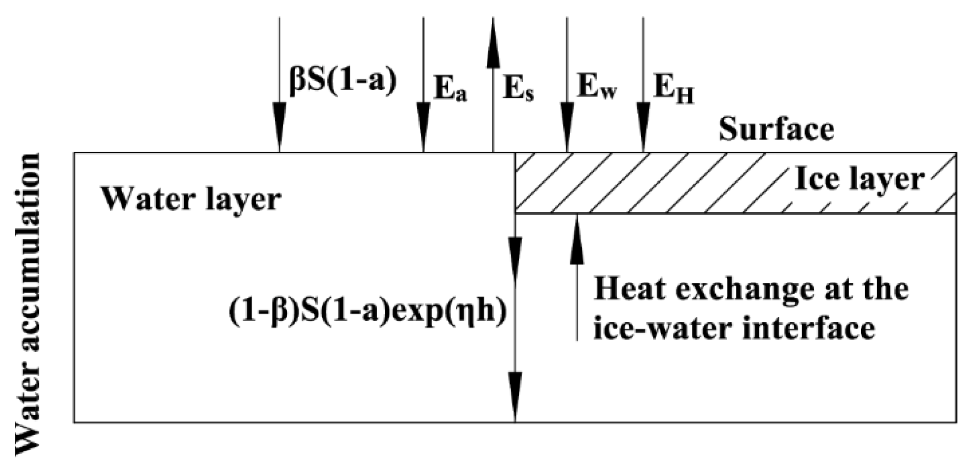
Each heat value in the left side of the equation (2) can be obtained directly by observations and calculated by formula and different models of lake [20].
Where, is the heat received at surface of water in unit time, is the surface heat exchange coefficient, is the equilibrium temperature; is surface water temperature; is the surface area of reservoir. and is expressed as:
Where, is the curve slope of water vapor pressure-temperature,, and are saturation and actual vapor pressure respectively,
and are air temperature and dew point temperature respectively; is the wind function related to evaporation; is the absorption coefficient of water surface to solar radiation; is the sun radiation reaching water surface.
The thermal balance at surface is also affected by flow conditions of water. Due to the density of water being a function of temperature as the Figure 2, according to the difference of water temperature, different density of water flows into different position. New energy is brought to the surface layer with the water flowing to the surface.
2.2. Frozen surface boundary
Ignoring the snow, there are two kinds of method to calculate thermal boundary at the frozen surface of water including formula and energy balance. Ashton [21] thought ice surface temperature is same as air temperature. Sydor [22] simulated ice growth through taking the measured water temperature under the ice as the thermal boundary.
In addition, more methods using energy balance method to calculate the frozen surface of pond are widely used.
Water is gradually frozen from the surface to lower as the surface reaches freezing temperature. And ice begins to melt, when the accumulated heat of ice reaches above 0℃. When water accumulation is completely frozen, heat is transferred from air and soil under water to ice. When water accumulation is not completely frozen, heat is transferred from high temperature and water to ice. So there is usually freezing in one direction from up to down and melting in two direction from up and down to middle position in permafrost regions [23].
Heat exchanges between ice-gas and ice-water is important during the process of freezing and melting. These heat exchanges above and the change of water temperature are affected by meteorological factors such as accumulated negative temperature, sunshine and wind speed, and controlled by convection and phase transition of water [24]. So icing time is related with accumulated air temperature, freezing time, and the area and depth of water. At the early stage of ice growth, the heat exchange between ice and air temperature is relatively large and the growth rate is fast. As ice layer becomes thicker, the heat exchange between air and ice are decreased, so the growth rate is stable. The thickness of ice is related to the average daily temperature and freezing time in cold season. Burn obtained the relationship between ice thickness and mean temperature in winter is linear by the measured data of Todd Lake in Canada [25].
3. Water temperature
3.1. Empirical law
The empirical methods of water temperature calculation can be divided into two types, which is the calculation method based on the boundary temperature of water and the vertical average temperature of water. The vertical temperature distribution of water is shown as Figure 3. Zhang calculated the vertical water temperature each month, according to the water temperature distribution of reservoir surface and bottom [26].
Where, is the vertical water temperature related to depth y, is the reservoir surface temperature, is the reservoir bottom temperature, x, n is a function related to month.
Chen [27] observed that the water temperature of reservoir mainly changed in the vertical direction, especially in summer, the temperature difference in vertical can be more than 10℃ based on the temperature measurement data of Miyun Reservoir in Beijing for two years.
But the empirical formula of water temperature obtained from measured data has particularity, ignoring the factors such as water flow, local meteorological conditions, wind mixing and so on. However, the referring factors can be taken into mathematical model by theoretical way, since its calculation results is more accurately, the mathematical model method may be more practical and universal.
3.2. Mathematical model method
The research on mathematical model of water accumulation temperature originated in 1930s. At that time, a large number of measured data of reservoir water temperature were analyzed in USA, and the stratification of water temperature was mainly reflected in the vertical direction. The diffusion model based on convection-diffusion is based on this assumption, the longitudinal and transverse temperature changes are ignored, and vertical water temperature stratification is considered, and all the elements of inflow in the same water layer are basically the same. Based on the convection-diffusion theory, WRE and MIT one-dimensional mathematical models were put forward successively in the 1960s. In the model, it is assumed that the reservoir is composed of mixed homogeneous horizontal isothermal thin layers, and the heat transfer only occurs between the adjacent horizontal thin layers, and the external flow flows into the water layer unit with the same pre support density [29,30].
The energy equation is
Where, T is the water temperature of unit layer ; is the inflow temperature ; A is the unit level area ; B is the average width of the unit layer ; is the vertical temperature diffusivity ; is the density of water , is a function of temperature; C is the Specific Heat Capacity of water ; is the solar radiation flux ; is the inflow velocity ; is the outflow velocity ; is the vertical flow through the upper boundary of the element ; N is the surface unit; is the volume of surface unit ; is the vertical flow through the interface between layer N and layer N-1 ; is the heat absorbed by the surface water through the water air interface .
In the middle and late of 1970s, the distribution of vertical water temperature was proposed considering the inflow and outflow of reservoir, and the influence of wind based on the total energy. In 1975, Stefan and Ford proposed MLTM model based on this theory [31]. In 1978, Imberger proposed the DYRESM model [32] suitable for simulating the temperature and salinity changes of reservoirs, and introduced the concept of mixed layer for the first time, which can simulate the distribution of reservoir inflow and outflow, water temperature and salinity at the same time. Since 1980, the mixed layer model has been widely used and improved because of its good characteristics of simulating water temperature and water quality. Some models have been applied to the study of water temperature in lakes and other ponding types. Although the mixed layer model increases the migration of turbulent kinetic energy compared with the previous diffusion model, the study of diffusion in the lower layer of ponding is fuzzy and has poor universality. It can be seen from the equation that the key to the water temperature distribution is the selection of vertical diffusion coefficient. Therefore, the improvement of water temperature numerical model is embodied in the treatment of vertical diffusion coefficient. Some models set the vertical diffusion coefficient as constant according to the focus of research problems, and more empirical formulas of vertical diffusion coefficient have been proposed, and various improved water temperature models have been applied.
With the gradual development of one-dimensional water temperature model, researchers have successively proposed two-dimensional or even three-dimensional water temperature model. The two-dimensional model integrates the input in term of N-S equation transversely and obtains the longitudinal and vertical water temperature distribution. In 1975, Edinger developed the earliest two-dimensional model LARM [33]. After that, two-dimensional water temperature models are proposed. Based on the energy balance and the vertical one-dimensional hybrid model. Farrell and Heinz [34] introduced k-ᵋ model into the simulation of reservoir density flow (k-ᵋ model is a mathematical treatment of water momentum equation), which can well simulate the characteristics of reservoir density flow, such as submergence, vertical vortex and temperature stratification. Young [35] proposed a two-dimensional model of turbulent diffusion of momentum and heat under different vertical empirical formulas. By using numerical software, a universal multi-dimensional prediction model of reservoir water temperature was established, which considered the factors of water surface heat exchange, reservoir inflow, reservoir discharge, reservoir water level and storage capacity change greatly. The three-dimensional model is based on the turbulence model, which considers the temperature changes in the transverse, longitudinal and vertical directions at the same time, and the heat transport equation and turbulence equation are coupled to solve. Due to the relatively large workload of 3D model calculation, it is not widely used in practice. By comparing the simulated and measured results of water temperature in the water accumulation, it is concluded that the variation of water accumulation temperature is related to its internal diffusion coefficient, and indirectly affected by the density of water under the action of temperature. In winter, the bottom temperature of deep water is high, and the heat is transferred to the upper part; in summer, the heat is transferred from the surface to the bottom, and the temperature from the surface to the bottom shows a linear or nonlinear trend. In the process of melting and freezing, the internal temperature stratification is obvious.
4. Phase change in pond
4.1. Empirical law
The empirical method is based on the measured data, which is from field observation and indoor test data. The method was improved continuously and according to the theory of water flow, thermal conduction, and the ice forming [36]. From the measured reservoir temperature data, it showed that the ice temperature near the ice surface is the same as the total radiation on the ice surface, and the closer the water temperature is to the ice bottom, the faster the water temperature decreases [37]. Temperature of static water condition is the main factor affecting ice condition, ice thickness is linearly related to accumulated hourly negative temperature. And water depth affects the start time of initial ice formation, but has little effect on the thermal change of ice. In the early stage of ice formation, the surface water body loses heat quickly and falls to freezing point to form ice needle ice. During freezing period, the bottom layer of ice layer crystallizes continuously under the heat conduction in the ice and the heat balance in the water to realize the of ice growth [38]. In the growth period, the temperature in the ice layer is basically linear distribution, and the slope of ice temperature increases with the decrease of temperature. The distribution of water temperature under ice during melting ice is basically unchanged, and the vertical temperature difference is mainly concentrated in the surface water body. It is shown that the water body is in a static state in the indoor experiment, and the heat exchange between the ice surface and the atmosphere is mainly affected by the temperature and relative humidity, and the icing only occurs at the interface of ice water. In view of the limitations of field measurement and model test, it can not be used directly and widely, and the water temperature calculation is nonlinear during phase transition. More mathematical models of water phase transition icing have been proposed one after another.
4.2. Mathematical model method
In the ice mathematical model, the development of river ice is better than that of reservoir ice [39]. The first one-dimensional vertical Chen-Orlob water temperature model considering icing was proposed in Carlson 1977, However, due to the lack of stability, it is difficult to simulate the of icing and melting process [40]. CE-QUAL-R1 model was proposed in Ashton 1982 to simulate the water temperature distribution under the ice layer [41]. In 1984, one dimensional unsteady river ice model was proposed, this model takes into account the variation of ice and density along the process [42,43]. The existing 1 and 2 dimensional ice mathematical model has developed relatively mature, Classic RICE models. Lal and Shen [44] improved and validated and applied in practice, Shen also proposed to replace the critical velocity in the RICE model with ice transport capacity, RECEN model for simulating ice transport and accumulation in ice cap. The temperature distribution models of the water layer and the lower soil layer after freezing under the heat exchange of each meteorological factor and the bottom of the water accumulation were established [45]. The empirical formulas and parameters in the above model were refined in Fang and Stefan in 1994 [46]. Fang [47] assumed that each water layer produces a heat exchange with the bottom of the water in 1996, the water temperature and ice growth were simulated for a long time. With the development of one-dimensional model, the two-dimensional icing model has been developed accordingly. Shen [48] proposed two-dimensional river ice mathematical models considering three modules: hydrodynamic force, ice transport and ice mass conservation. Although the research of river ice model has made great progress, but because of the complexity of the mechanics of the river itself, in the process of calculating temperature, various physical mechanism processes, such as hydrodynamic, thermal and phase transition, Therefore, there will still be more problems in the development of river ice model. The key to simulate the icing of rivers and lakes lies in the consideration and treatment of ice water and ice gas interface.
For the study of reservoir ice condition, it is still in the initial stage. At present, in the reservoir ice model, the Stefan classical assumption is used to determine the ice surface temperature. It is considered that the ice surface temperature is equal to the air temperature and the water temperature under the ice is linearly assumed [49]. In addition to meteorological conditions, the reservoir capacity and the flow into the reservoir are also the main factors affecting the water temperature of the reservoir. Hence, the ice condition in the reservoir is affected by many factors, such as meteorological conditions, reservoir morphology, operation mode and hydrodynamic conditions, and the icing mechanism is relatively complex [49]. Reservoir surface ice is mostly formed in winter night temperature difference, the surface is less than 0℃, ice formation begins on the shore, as the temperature decreases, more ice is gradually formed at the deep level of reservoir. Xing Fang [50] considering the influence of wind speed, a lake ice model was established to calculate the ice thickness by using the heat lost from water cooling.
5. Heat exchange between the bottom of water accumulation and the underlying soil
The research and development of water temperature calculation model shows that the heat situation in water accumulation depends on the energy exchange between the water and the environment. Therefore, the water, the upper atmosphere and a part of the adjacent soil layer should be taken to calculate the complete calculation model. Especially for the shallow water, the influence of the heat exchange of the bottom soil layer on the heat distribution in water accumulation can not be ignored. In the previous calculation methods of water temperature distribution in lakes and reservoirs, the thermal effect of soil layer was also considered. In 1972, the calculation model of temperature distribution in water and underwater sediment by finite difference method was established [51]. The thermal effects between the water accumulation and the soil layer are also mutual, especially when studying the influence of water accumulation on nearby projects, the soil layer at the water bottom should be considered in calculation and analysis. Stepanenko [52] used the plant soil model [53] to analyze the heat and water exchange between the bottom of the ponding and the soil. Xing Fang [54] proposed a modified ponding model considering the heat exchange between the ponding and the bottom sediments, indicating that the change of bottom water temperature can affect the depth of 10 meters.
Water depth and water contact of soil affect the degree of water temperature affected by external changes and the heat exchange between the bottom and soil. The measured bottom water temperature of lake shows that the lake edge temperature is lower than that of the inner deep water in the cold season, while the temperature at the lake edge is higher than that of the inner deep water in the warm season. The heat exchange between the lake bottom and the soil layer is greater than that of the internal deep water. The bottom temperature varies in the horizontal direction due to the influence of water depth and heat exchange between water and soil [55]. In the alpine environment, taking permafrost region as an example, the relationship between water depth and freezing depth will also affect the lower soil layer affected by the heat of ponding, and the temperature of the bottom layer of ponding determines the development of its lower melting zone [56,57]. When the depth of water is less than the freezing depth, the water bottom temperature is less than 0 ℃ [58]. However, when the water depth is greater than or equal to the freezing depth, the water accumulation in winter is not completely frozen or the bottom of the cold season is frozen, and the temperature is still higher than 0℃. The long-term effects of the above two scenarios will drive the bottom soil layer of water accumulation to gradually form a melting layer [59]. If the accumulated water does not exist for a long time and the temperature at the bottom does not change recently, the lower soil layer and the bottom of the ponding reach the thermal balance, and the lower melting layer will not develop any more [60,61,62]. However, if the accumulated water exists for a long time or the bottom temperature changes obviously due to the external temperature, such water will have a great impact on the development of the surrounding permafrost. By measuring and simulating the heat budget at different positions of the water accumulation, it is found that the lower part of the water has formed a through hot melt zone, and the surrounding frozen soil has degenerated [59]. The results show that the long-term existence of the thermokrast lake in cold region can be regarded as the heat source of the permafrost around it [63]. Therefore, the heat exchange between water and soil should be considered in the water temperature calculation model, and the heat exchange between water and soil can not be ignored when studying the heat effect of water accumulation, and the heat impact caused by water is also affected by the external environment, geological conditions, water accumulation type and other factors.
6. Discussion
There is vertical temperature stratification in the water accumulation, which can be divided into mixed type, stable type and transition type between them because of the degree of stratification. For the mixed type, water temperature gradient in vertical direction is small and the bottom temperature varies little with surface temperature. For the stable type, there are layers of variable temperature, oblique temperature and average temperature from the upper to the lower, and the surface water temperature changes faster than the middle and lower layers. The transition type has the temperature characteristic of the two types above. When the surface is frozen, the ice temperature is distributed with temperature gradient, and the water layer under ice still accords with the distribution characteristics of above water body.
The main factors of water temperature stratification are surface absorption heat, wind speed, solar short wave radiation, heat conduction and buoyancy convection in the water accumulation, which are determined by the environment, climate, depth, scale and thermal parameters of the pond. The surface absorption heat is the source power of the water accumulation. The wind speed can affect the kinetic energy of surface layer diffusing heat to lower layer. The solar short wave radiation absorbed in every layer affects the internal energy exchange of water. Besides that, the density of water is a nonlinear function of temperature, and the density of about 4℃ is the largest. When there is an unstable temperature stratification in the water accumulation, the difference of density can form natural buoyancy flow, which causes the corresponding water flow and promotes the temperature change in the pond. The depth of water not only changes the influence of solar radiation, but also changes the effect degree by the surrounding soil. Shallow water is more affected by solar radiation and surrounding soil. The area of water accumulation can affect the flow state of water and the heat transfer ability of water and the degree of natural buoyancy convection. Moreover, the water temperature distribution is also affected by the inlet and outlet water temperature and velocity. The external forced inflow will cause additional energy and momentum exchange in the pond. Then the redistribution of internal energy of water accumulation is affected to change the state of water temperature distribution.
When the water is frozen, the latent heat of phase change between ice and water and the movement of interface will affect the distribution of water temperature. The ice layer is a simple solid heat transfer and the attenuation coefficient of solar short wave radiation is different from that of water layer. Therefore, the influence factors considered in the temperature distribution of water accumulation with icing process include ice melting period, ice thickness and thermodynamic parameters of ice. The energy transfer process and law after freezing should also consider the influence of the depth and area of the water accumulation. The shallow water is greatly affected by the heat exchange between the soil and water, and the water accumulation area will affect the icing sequence of the surface layer.
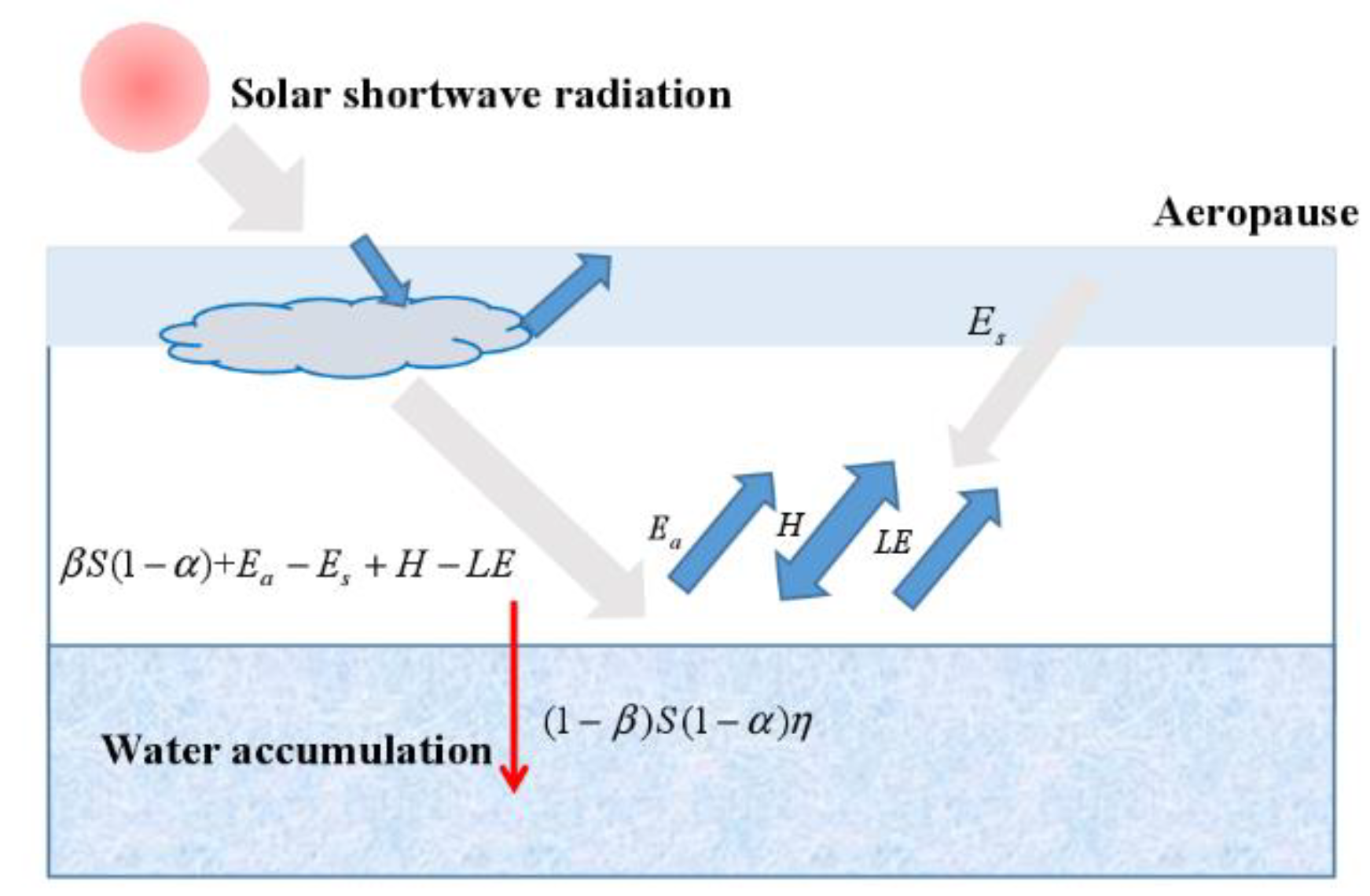
The water accumulation in permafrost region also involves phase transformation. So these factors above which can affect the water temperature change are also be considered in permafrost regions, in order to make the water temperature calculation more accurate. The key to the calculation of water accumulation in cold regions lies in Figure 4. They are including that the energy exchange at the interface of water and air, including the energy exchange at the interface of water and air, the heat transfer in water accumulation and the energy exchange between soil and water bottom. For the interface of water and air, it is important to calculate the surface energy balance of water considering the meteorological elements above the surface, and there is difference between the surface of water and ice. For the heat transfer in water accumulation, it is important to make an analysis of water temperature stratification taking the actual buoyancy flow into account and the solution of melting and freezing of ice. The heat transfer in ice layer is solid and that in water is fluid, and ice always floats on the surface of water. In addition, the solar short wave radiation will exist in each water layer as a heat source in the heat exchange inside the water accumulation. The heat exchange between water accumulation bottom and permafrost below pond is key to calculate water temperature.
7. Conclusion
As a kind of boundary of the earth, water accumulation changes the energy exchange between the earth and the atmosphere, affects the changes of the surrounding environment, and indirectly affects the stability of adjacent projects. In order to deeply analyze its impact on local environment and engineering, it is necessary to define the response of water accumulation to climatic conditions, that is, to calculate and analyze the internal temperature of water accumulation with time and changes of external conditions. Taking lakes and reservoirs as the research objects, this paper summarizes the methods, mechanisms and application conditions of surface and internal temperature calculation and analysis of water accumulation. However, for the special soil environment in permafrost regions, the calculation and analysis of water heat and its impact on frozen soil engineering are still in the initial stage, and there are many problems to be studied in deep.
1. It is more applicable to calculate the water surface temperature by energy balance method, which includes solar short wave radiation, net long wave radiation, sensible heat and latent heat. The mechanism and influence degree of various factors on the surface temperature of water accumulation can be discussed in depth, which is conducive to accurate prediction of water temperature.
2. The depth and area of water accumulation will affect the water temperature distribution by affecting the internal flow. Therefore, it is necessary to analyze the variation law of water temperature and its influence on the thermal state of the lower soil layer from the perspective of water accumulation scale.
3. The existence of water accumulation in special areas not only affects the environment, but also affects the stability of surrounding engineering structures. These impacts are also related to the condition and existence time of water accumulation. Therefore, it is necessary to analyze the impact of water accumulation on the underlying soil based on the response of water accumulation to climate under different existing time.
Acknowledgments
This work has been supported by Open Fund of State Key Laboratory of Frozen Soil Engineering (SKLFSE202120), Hongliu outstanding young talents support program of Lanzhou University of Technology (062006).
References
- Lin, Z.; Niu, F.; Liu, H.; Lu, J. Hydrothermal processes of alpine tundra lakes, beiluhe basin, Qinghai-Tibet plateau. Cold. Reg. Sci. Technol. 2011, 65, 446–455. [Google Scholar] [CrossRef]
- Luo, J.; Niu, F.; Lin, Z.; Liu, M.; Yin, G. Thermokarst lake changes between 1969 and 2010 in the Beilu River Basin, Qinghai–Tibet Plateau, China. Sci. Bull. 2015, 60, 556–564. [Google Scholar] [CrossRef]
- Banimahd, S.; Zand-Parsa, S. Simulation of evaporation, coupled liquid water, water vapor and heat transport through the soil medium. Agr. Water. Manage. 2013, 130, 168–177. [Google Scholar] [CrossRef]
- Burn, C. Tundra lakes and permafrost, Richards Island, western Arctic coast, Canada. Can. J. Earth Sci. 2002, 39, 1281–1298. [Google Scholar] [CrossRef]
- Lin, Z.; Niu, F.; Xu, Z.; Xu, J.; Wang, P. Thermal regime of a thermokarst lake and its influence on permafrost, Beiluhe Basin, Qinghai-Tibet Plateau. Permafrost. Periglac. 2010, 21, 315–324. [Google Scholar] [CrossRef]
- Peng, E.; Sheng, Y.; Hu, X.; Wu, J.; Cao, W. Thermal effect of thermokarst lake on the permafrost under embankment. Adv. Clim. Change. Res. 2021, 12, 76–82. [Google Scholar] [CrossRef]
- Hinkel, K.; Lenters, J.; Sheng, Y.; Lyons, E.; Beck, R.; Eisner, W.; Maurer, E.; Wang, J.; Potter, B. Thermokarst Lakes on the Arctic Coastal Plain of Alaska: Spatial and Temporal Variability in Summer Water Temperature. Permafrost. Periglac. 2012, 23, 207–217. [Google Scholar] [CrossRef]
- Wen, Z.; Yang, Z.; Yu, Q.; Wang, D.; Ma, W.; Niu, F.; Sun, Z.; Zhang, M. Modeling thermokarst lake expansion on the Qinghai-Tibetan Plateau and its thermal effects by the moving mesh method. Cold. Reg. Sci. Technol. 2016, 121, 84–92. [Google Scholar] [CrossRef]
- Gao, Z.; Niu, F.; Wang, Y.; Luo, J.; Lin, Z. Impact of a thermokarst lake on the soil hydrological properties in permafrost regions of the Qinghai-Tibet Plateau, China. Sci. Total. Environ. 2017, 574, 751–759. [Google Scholar] [CrossRef]
- Chen, L.; Yu, W.; Zhang, T.; Yi, X. Asymmetric talik formation beneath the embankment of Qinghai-Tibet Highway triggered by the sunny-shady effect. Energy. 2023, 266, 126472. [Google Scholar] [CrossRef]
- Kokelj, S.; Lantz, T.; Kanigan, J.; Smith, S.; Coutts, R. Origin and polycyclic behaviour of tundra thaw slumps, Mackenzie Delta region, Northwest Territories, Canada. Permafrost. Periglacial. 2009, 20, 173–184. [Google Scholar] [CrossRef]
- Peng, E.; Hu, X.; Sheng, Y.; Zhou, F.; Wu, J.; Cao, W. Establishment and Verification of a Thermal Calculation Model Considering Internal Heat Transfer of Accumulated Water in Permafrost Regions. Front. Earth. Sci-Switz. 2021, 9, 733483. [Google Scholar] [CrossRef]
- Calmels, F.; Delisle, G.; Allard, M. Internal structure and the thermal and hydrological regime of a typical lithalsa: significance for permafrost growth and decay. Can. J. Earth. Sci. 2008, 45, 31–43. [Google Scholar] [CrossRef]
- Chen, L.; Fortier, D.; McKenzie, J.; Voss, C. I. , & Lamontagne-Hallé, P. Subsurface porewater flow accelerates talik development under the Alaska Highway, Yukon: A prelude to road collapse and final permafrost thaw? Water Resour Res. 2023, 59. [Google Scholar]
- Fang, X.; Stefan, H. Long-term lake water temperature and ice cover simulations/measurements. Cold. Reg. Sci. Technol. 1996, 24, 289–304. [Google Scholar] [CrossRef]
- Romanovsky, V.; Osterkamp, T. Effects of unfrozen water on heat and mass transport processes in the active layer and permafrost. Permafrost. Periglac. 2000, 11, 219–239. [Google Scholar] [CrossRef]
- Jorgenson, M.; Shur, Y. Evolution of lakes and basins in northern Alaska and discussion of the thaw lake cycle. J. Geophys. Res. 2007, 112, F02S17. [Google Scholar] [CrossRef]
- Chen, L.; Voss, C.; Fortier, D.; McKenzie, J. Surface energy balance of sub-Arctic roads and highways in permafrost regions. Permafrost Periglacial. 2021, 4, 681–701. [Google Scholar] [CrossRef]
- Stepanenko, V. Numerical modeling of heat and moisture transfer processes in a system lake–soil. Russ. Meteorol. Hydro+. 2005, 3, 95–104. [Google Scholar]
- Lykossov, V.; Volodin, E. Parameterization of heat and moisture transfer in the soil-vegetation system for use in atmospheric general circulation models: 2. Numerical experiments in climate modeling. Izv. Atmos. Ocean. Phy+. 1998, 5, 559–569. [Google Scholar]
- Ashton, G. ‘’Heat transfer to river ice covers’’. In Proc. Presented at the East snow conference, 30th annual meeting, Amherst, Massachusetts, 1973, Feb. 8-9.
- Sydor, M. Ice growth in duluth-superior harbor. J. Geophys. Res. 1978, 83. [Google Scholar] [CrossRef]
- Fang, X.; Ellis, C.; Stefan, H. Simulation and observation of ice formation (freeze-over) in a lake. Cold. Reg. Sci. Technol. 1996, 24, 129–145. [Google Scholar] [CrossRef]
- Lei, Y.; Liao, R.; Su, Y.; Zhang, X.; Liu, D.; Zhang, L. Variation Characteristics of Temperature and Rainfall and Their Relationship with Geographical Factors in the Qinling Mountains. Atmosphere. 2023, 14, 696. [Google Scholar] [CrossRef]
- Burn, C. Lake-bottom thermal regimes, western Arctic coast, Canada. Permafrost. Periglac. 2005, 16, 355–367. [Google Scholar] [CrossRef]
- Dafa, Z. Analysis and estimation of reservoir water temperature. J. Hydrol. 1984, 21–29. [Google Scholar]
- Li, Y.; Zhang, B. Study on vertical water temperature model for miyun reservoir. J. Hydrodyn. 1998, 4, 75–83. [Google Scholar]
- Hong, J. Discussion on Calculation method of reservoir water temperature. J. Hydraul. Eng. 1999, 2, 63–72. [Google Scholar]
- Nwokolo, S.; Proutsos, N.; Meyer, E.; Ahia, C. Machine Learning and Physics-Based Hybridization Models for Evaluation of the Effects of Climate Change and Urban Expansion on Photosynthetically Active Radiation. Atmosphere. 2023, 14, 687. [Google Scholar] [CrossRef]
- Patrick, M.; Duguay, C.; Flato, G.; Rouse, W. Simulation of ice phenology on Great Slave Lake, Northwest Territories, Canada. Hydrol Process. 2002, 26, 3691–3706. [Google Scholar]
- Gu, R.; Stefan, H.G. Year-round temperature simulation of cold climate lakes. Cold Reg Sci Technol. 1990, 2, 147–160. [Google Scholar] [CrossRef]
- Hostetler, S. Simulation of lake ice and its effect on the late-Pleistocene evaporation rate of lake Lahontan. Climate Dynamics. 1991, 6, 43–48. [Google Scholar] [CrossRef]
- Henderson-Sellers, B. New formulation of eddy diffusion thermocline models. Appl. Math. Model. 1985, 9, 441–446. [Google Scholar] [CrossRef]
- Hostetler, S.; Bates, G.; Giorgi, F. Interactive coupling of a lake thermal model with a regional climate model. Science. 1993, 263, 665–667. [Google Scholar] [CrossRef]
- Young, Der-Liang Frank. "Finite element analysis of stratified lake hydrodynamics." Environmental Fluid Mechanics: Theories and Applications. ASCE, 2002, 339-376.
- Р.В.Dorchenko. Ice conditions of rivers in the Soviet Union. 1991.
- Hostetler, S.; Bartlein, P. Simulation of lake evaporation with application to modeling lake level variations of Harney-Malheur Lake, Oregon. Water Resoures Research. 1990, 26(10), 2603–2612. [Google Scholar]
- Paily, P.; Macagno, E.; Kennedy, J. Winter-regime surface heat loss from heated streams. Research report. 1974. [Google Scholar]
- Yapa, P.D.; Shen, H.T. Unsteady Flow Simulation for an Ice-Covered River. J. Hydraul. Eng. 1986, 112, 1036–1049. [Google Scholar] [CrossRef]
- De Bruin, H.A.R.; Wessels, H.R.A. A model for the formation and melting of ice on surface waters. Journal of Applied Maeorology. 1988, 27:164- 173.
- Shen, H.; Wang,D. ; Lal, A. Numerical Simulation of River Ice Processes. Journal of Cold Regions Engineering. 1995, 3, 107–118. [Google Scholar] [CrossRef]
- Shen, H.; Wang, D.; Lal, A.M.W. Numerical Simulation of River Ice Processes. J Cold Reg Eng. 1995, 9, 107–118. [Google Scholar] [CrossRef]
- Zufelt, J.; Ettema, R. Fully Coupled Model of Ice-Jam Dynamics. J Cold Reg Eng. 2000, 14, 24–41. [Google Scholar] [CrossRef]
- Lal, A.; Shen, H. Mathematical Model for River Ice Processes. J Hydraul Engasce. 1991, 117, 851–867. [Google Scholar] [CrossRef]
- Gu, R.; Stefan, H. Year-round temperature simulation of cold climate lakes. Cold Reg Sci Technol. 1990, 18, 147–160. [Google Scholar] [CrossRef]
- Fang, X.; Stefan, H. Temperature and dissolved oxygen simulations in a lake with ice cover. Project Report 356, St. Anthony Falls Hydraulic Laboratory, University of Minnesota, Minneapolis, MN. 1994.
- Fang, X.; Stefan, H.G. Long-term lake water temperature and ice cover simulations/measurements. Cold Reg Sci Technol. 1996, 24, 289–304. [Google Scholar] [CrossRef]
- Shen, H.; Lu, S. Dynamics of River Ice Jam Release.Proceedings of the International Conference on J Cold Reg Eng. 1996, 594-605.
- Tuo, Y.; Deng, Y.; Huang, F.; Li, J.; Liang, R. Study on the Coupled Mathematical Model of the Vertical 1D Temperature and Ice Cover in the Reservoir. Journal of Sichuan University. 2011. [Google Scholar]
- Fang, X.; Ellis, C.; Stefan, H. Simulation and observation of ice formationin a lake. Cold Reg Sci Technol. 1996, 24, 129–145. [Google Scholar] [CrossRef]
- Carlson, R.; Fox, P.; LaPerriere, J. Development of an Operational Northern Aquatic Ecosystem Model: Completion Report. University of Alaska, Institute of Water Resources. 1977.
- Stepanenko, V. Numerical modeling of heat and moisture transfer processes in a system lake – soil. Russ Meterol Hydro+. 2005, 3, 95-104.
- Volodin Е.; Lykosov V. Parameterization of processes of heat and moisture transfer in a vegetation-soil system for Atmospheric Global Circulation modeling. 1. Description and experiments with local observational data//Izvestiya RAN. Physics of Ocean and Atmosphere. 1998, 34, 453-465.
- Xing, F.; Stefan, H.G. Long-term lake water temperature and ice cover simulations/measurements. Cold Reg Sci Technol. 1996, 24, 289–304. [Google Scholar]
- Lin, Z.; Niu, F.; Liu, H.; Lu, J. Hydrothermal processes of Alpine Tundra Lakes, Beiluhe Basin, Qinghai-Tibet Plateau. Cold Reg Sci Technol. 2011, 65, 446–455. [Google Scholar] [CrossRef]
- Lin, Z.; Niu, F.; Ge, J. ; Variation characteristics of thaw lakes in permafrost regions of the Qinghai-Tibet Plateau and its influence on the thermal state of permafrost. Journal of Glaciology and Geocryology. 2010, 2, 341–349. [Google Scholar]
- Lin, Z.; Mm, F.; Xu, Z.; Xu, J.; Wang, P. Thermal Regime of a Thermokarst Lake and its Influence on Permafrost, Beiluhe Basin, Qinghai-Tibet Plateau. Permafrost Periglacial. 2010, 4, 315–324. [Google Scholar] [CrossRef]
- Ling, F.; Zhang, T. Numerical simulation of permafrost thermal regime and talik development under shallow thaw lakes on the Alaskan Arctic Coastal Plain. J GEOPHYS RES. 2003, 16, 26–36. [Google Scholar] [CrossRef]
- Lin, Z.; Niu, F.; Hua, L.; Lu, J. Hydrothermal processes of Alpine Tundra Lakes, Beiluhe Basin, Qinghai-Tibet Plateau. Cold Reg Sci Technol. 2011, 65, 446–455. [Google Scholar] [CrossRef]
- Johnston, G.; Brown, R. Some observations on permafrost distribution at a lake in the Mackenzie Delta N.W.T. Canada. Arctic. 1964, 17, 162–175. [Google Scholar] [CrossRef]
- Johnston, G.; Brown, R. Occurrence of permafrost at an arctic lake. Nature (London). 1966, 211, 952–953. [Google Scholar] [CrossRef]
- Smith, M. Permafrost in the Mackenzie Delta, Northwest Territories. Geological Survey of Canada. 1976, 75–28. [Google Scholar]
- Hu, X.; S, Y.; Li, J. Progress in the research of the influence of ponding by embankment on the stability of embankment in perma frost regions. J Glaciol Geocryol. 2014, 36, 876–885. [Google Scholar]
Figure 2.
Water density with temperature.
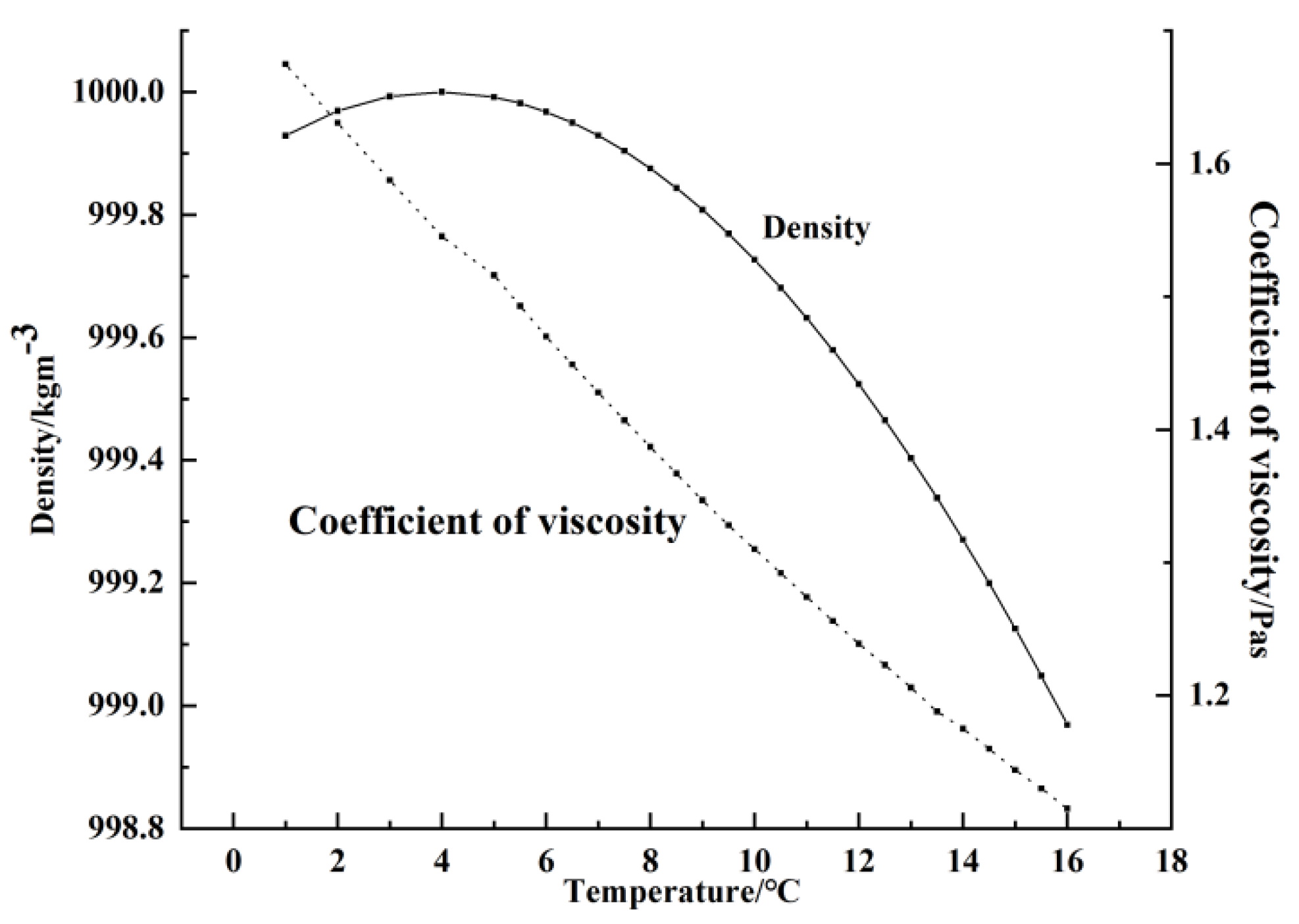
Figure 3.
Stratified distribution of water temperature.
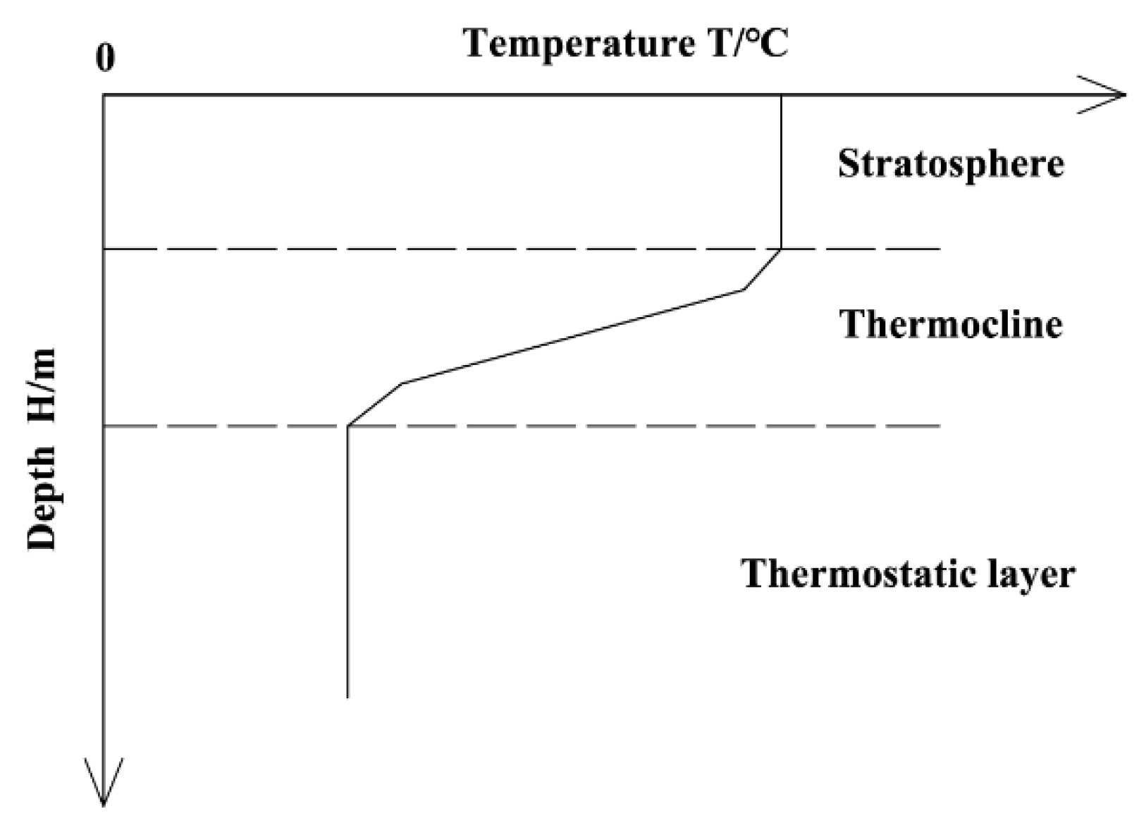
Figure 4.
Heat exchange between air and water.
Disclaimer/Publisher’s Note: The statements, opinions and data contained in all publications are solely those of the individual author(s) and contributor(s) and not of MDPI and/or the editor(s). MDPI and/or the editor(s) disclaim responsibility for any injury to people or property resulting from any ideas, methods, instructions or products referred to in the content. |
© 2023 by the authors. Licensee MDPI, Basel, Switzerland. This article is an open access article distributed under the terms and conditions of the Creative Commons Attribution (CC BY) license (http://creativecommons.org/licenses/by/4.0/).
Copyright: This open access article is published under a Creative Commons CC BY 4.0 license, which permit the free download, distribution, and reuse, provided that the author and preprint are cited in any reuse.


