1. Introduction
1.1. Background and significance
In the field of industry, images may be partially shaded, lost, damaged, distorted, even unmeasurable due to such factors as detection principle, detection hardware, signal transmission, noises, external environments. This sometimes causes some incomplete signals which makes much adverse impact on the performance of the whole control system. Therefore, it is so critical for incomplete signals to synthesize, restore, repair, reconstruct or predict that it has become the hot topics in related fields. The typical one is image inpainting, which originates from the art restoration of old images.
The image inpainting is generally divided into traditional methods and deep learning methods [
1,
2,
3,
4,
5]. The traditional ones are mostly based on low-level expression of image semantics (including color, texture, grayscale, shape, constituent, etc.), that is, the incomplete part is often filled with similarity pixels or patches of existing images, or is diffused and multiplied by existing pixels. The methods are naturally on the basis of nearest neighbor searching, i.e., using patches or pixels to synthesize images, including exemplar-based texture synthesis methods, exemplar-based structure synthesis methods, diffusion-based methods, sparse representation methods [
1,
2,
3,
6,
7,
8], etc. The deep learning ones such as deep neural network, convolutional neural network, generative adversarial network (GAN) and auto-encoder [
4,
5,
9,
10,
11,
12,
13,
14,
15,
16] are best at obtaining sketchy results, which mostly focus on the medium-level or high-level semantics such as visual object and scene.
Up to now, unified standard for the evaluation of image inpainting hasn’t been made. Quantitative measurement and subjective qualitative judgment are common practices [
4,
5]. The former usually includes peak signal to noise ratio (PSNR) [
17] and structural similarity [
18]. In particular, there are many evaluations to judge the similarity of time series curves, such as dynamic time warping, longest common sub-sequence, edit distance on real sequence and so on [
19,
20,
21,
22].
The traditional methods of image inpainting are simple in general, but in practice they have some limits, including the small inpainting area, the difficulties in inpainting of complex mask areas and in achievement of global coordination. Deep learning methods have advantages in high-level semantic understanding. However, these methods are usually featured with a large number of training samples, complex models, poor real-time performance, high cost and rough numerical values, which are still in development. The methods above have been well applied in many fields and provide certain reference for this paper. However, the methods pay little attention to line-scan images and synthesis numerical precision, and many common evaluations are not suitable for this study either. With respect to industrial application of line-scan DE-XRT to identify materials based on the R_value (transparency natural logarithm ratio of low energy to high energy, which is related to the effective atomic number and density of materials), this paper focuses on the synthesis (inpainting) of signals which cannot be directly measured before attenuation within the range of material because such signals directly affect the calculation accuracy of R_value. Besides that, fine and high-efficiency identification and classification have become more and more dependent on improvement of the numerical precision of the synthetic signals and the real-time. Therefore, the method is of great significance to the sorting of non-ferrous metals, plastics and other solid wastes, as well as to the resources, environment and economy of modern society, and is also beneficial to the realization of the global strategic goal of "carbon peak and carbon neutralization".
1.2. Problem presentation
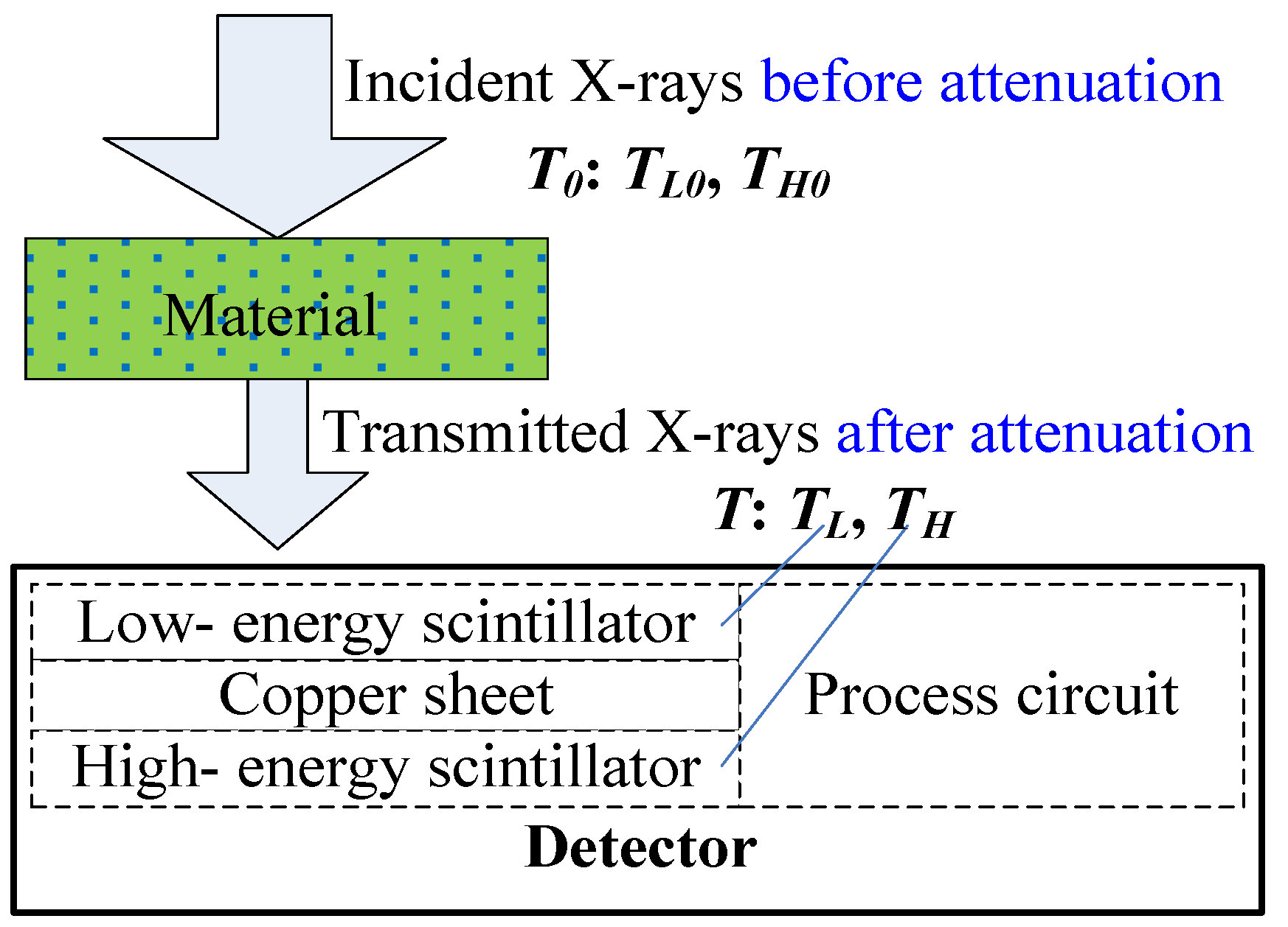
The schematic diagram of a single source continuous spectrum DE-XRT line-scan detection is shown in
Figure 1. The upper layer of the sandwich type detector is a low-energy scintillator and the lower layer is a high-energy scintillator. After the transmitted X-ray is converted by these scintillators and processed by the circuit, the low-energy value and the high-energy value of each pixel can be obtained at the same time. Between the upper and lower layers are copper sheets that can filter out most of the low-energy X-rays. The X-rays will attenuate when penetrating the material, and the signals after attenuation
T (the attenuated X-rays, the low-energy value is
TL and the high-energy value is
TH) can be obtained through the line-scan detector. But, if the signals before attenuation
T0 (the incident X-rays, the low-energy value is
TL0 and the high-energy value is
TH0) within the material range are also obtained by the detector, the detector itself will block and affect the X-ray signals, and foreign materials will be mixed in, which will affect the signal characteristics of the measured material and become complex and difficult to identify, so
TL0 and
TH0 cannot be measured directly. Nevertheless, the transparency of the above R_value is
TL/
TL0 at low-energy and
TH/
TH0 at high-energy, that is,
TL0 and
TH0 are necessary for the R_value calculation.
Appropriate filter (such as improved adaptive Kalman-median filter [
23]) can be adopted for signals after attenuation. The filtered signals can be updated in real-time with environmental changes, which basically remove high-frequency noises and retain the real low-frequency fluctuations of the signals. The synthesized signals before attenuation should also have these characteristics, so the calculation of R_value will be more accurate. According to the actual measurement in the laboratory, we have prepared two groups of typical data, that is, the influence of two processing methods of signals before attenuation (
T0) on the calculation of R_value is shown in
Table 1. In the table, the data of the first line are the proposed "true" values, and the calculated R_value is 1.7. The data of the second line simulate the case where low-frequency fluctuation of the signal occurs, for example, the signal after attenuation get increment by 40 values, while the
T0 signal before transmission does not follow (for example, only the average value of the previous period is taken, i.e., the traditional moving average filter is adopted). In this case, the calculation error of R_value is 0.54%. The data of the third line simulate the characteristics of following low-frequency fluctuations, which the signal
T0 before transmission also follows the signal
T after attenuation by 40 numerical increments. The calculation error of R_value is only 0.002 315% at this time, and the calculation accuracy of R_value is more than 200 times higher than that of the second line. Due to the ratio logarithm of R_value calculation, the error of signals before attenuation may be greatly amplified on R_value, so does the one of signals after attenuation. The higher the calculation accuracy of R_value, the finer the material identification.
1.3. Purpose and main contents
In view of the above reasons, it is necessary to properly synthesize the signals before attenuation in DE-XRT material identification. In addition, the line-scan DE-XRT image has a difference in vertical (forward/column) direction and horizontal (scanning/row) direction, that is, the vertical is a time series with continuity of signal change trend; the horizontal is spatial and has the fluctuation synchronization of the signals in the same row. Therefore, according to these requirements and characteristics, the purpose of this paper is to solve the problems of synthesis of unmeasurable signals before attenuation in DE-XRT, improve its numerical precision, and lay a foundation for improving the accuracy of R_value and material identification.
The main content of this paper is that for the synthesis of a column of signals, the historical statistical data (outside the material) of the recent mean and standard deviation (SD) in the same column and the measurable reference columns are used; simultaneously, the fluctuation of each synthesized pixel with the measurable signals of the reference columns in the same row is synchronized; smooth transition processing in the vicinity of the end points of the synthetic column is conducted. Each column of signals in the incomplete area are synthesized so as to finish the synthesis of all signals before attenuation within the material range. In addition, corresponding evaluations are proposed for the above synthesis results.
The method proposed in this paper has high precision of numerical synthesis and good real-time performance, which is conducive to high-speed and efficient in-line DE-XRT identification and separation of solid wastes. It can be extended to the fields of incomplete signals/image numerical high-precision synthesis of line-scan detectors, especially the synthesis of background signals with little fluctuations.
The rest of this paper is structured as follows:
Section 2 is materials and methods, including the parameters of experimental equipment, the synthesis ideas, methods and evaluations;
Section 3 is the results and discussion, including a column of synthesis curve, mask image synthesis and its comparison with deep convolutional generative adversarial networks (DCGAN) based inpainting method;
Section 4 is the conclusions.
2. Materials and methods
2.1. Setup and materials
The data acquisition and sorting system is composed of Spellman SRB401 X-ray source, Sens-Tech LINX-1605-301 line-scan energy integration detector, Advantech IPC-610MB-L industrial personal computer (IPC, Intel i7-2600 CPU with main frequency 3.4 GHz, 4 physical cores, 8 GB memory and window 7 64-bit operating system), belt line, etc. Visual Studio 2012 and MATLAB R2020a are used for development. The experimental parameters used are: 200 kV tube voltage, 2 mA tube current, 320×320 pixels with 16-bit depth in each frame image, corresponding to 1.6 mm (horizontal) × 1.2 mm (vertical), line speed of 1 m/s, and frame interval of 384 ms. Another of our research work described the system composition and the relationship between various operation parameters in detail [
24].
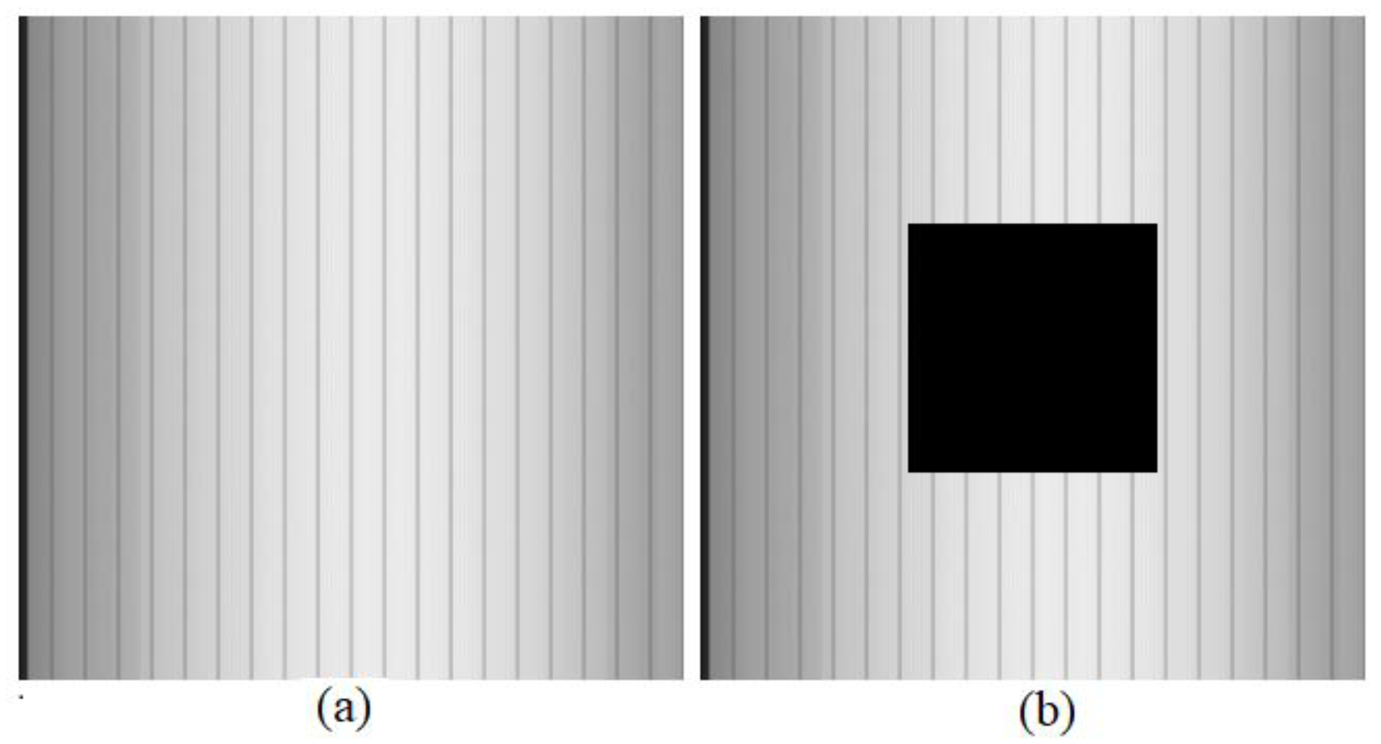
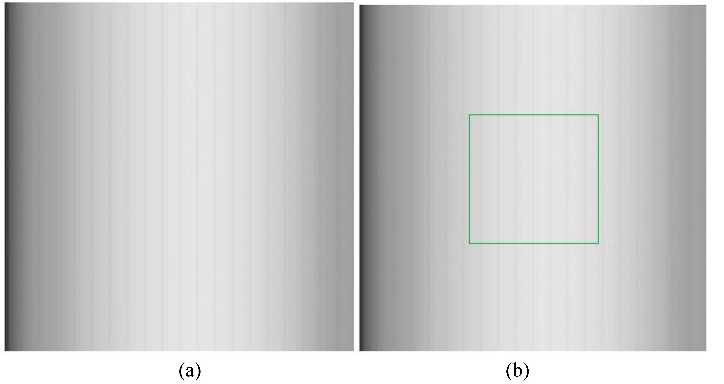
The original image used for the signal synthesis experiment is shown in
Figure 2a, which is a 320×320 pixels low-energy background (material free) image. The partially masked image is shown in
Figure 2b, which is a square area (assumed material range) with pixel coordinates from (101, 101) to (219, 219), that is, the incomplete part accounts for about 13.8% of the whole image.
2.2. Synthesis of signals before attenuation based on vertical and horizontal bidirectional context
2.2.1. Synthetic ideas and symbolic meaning
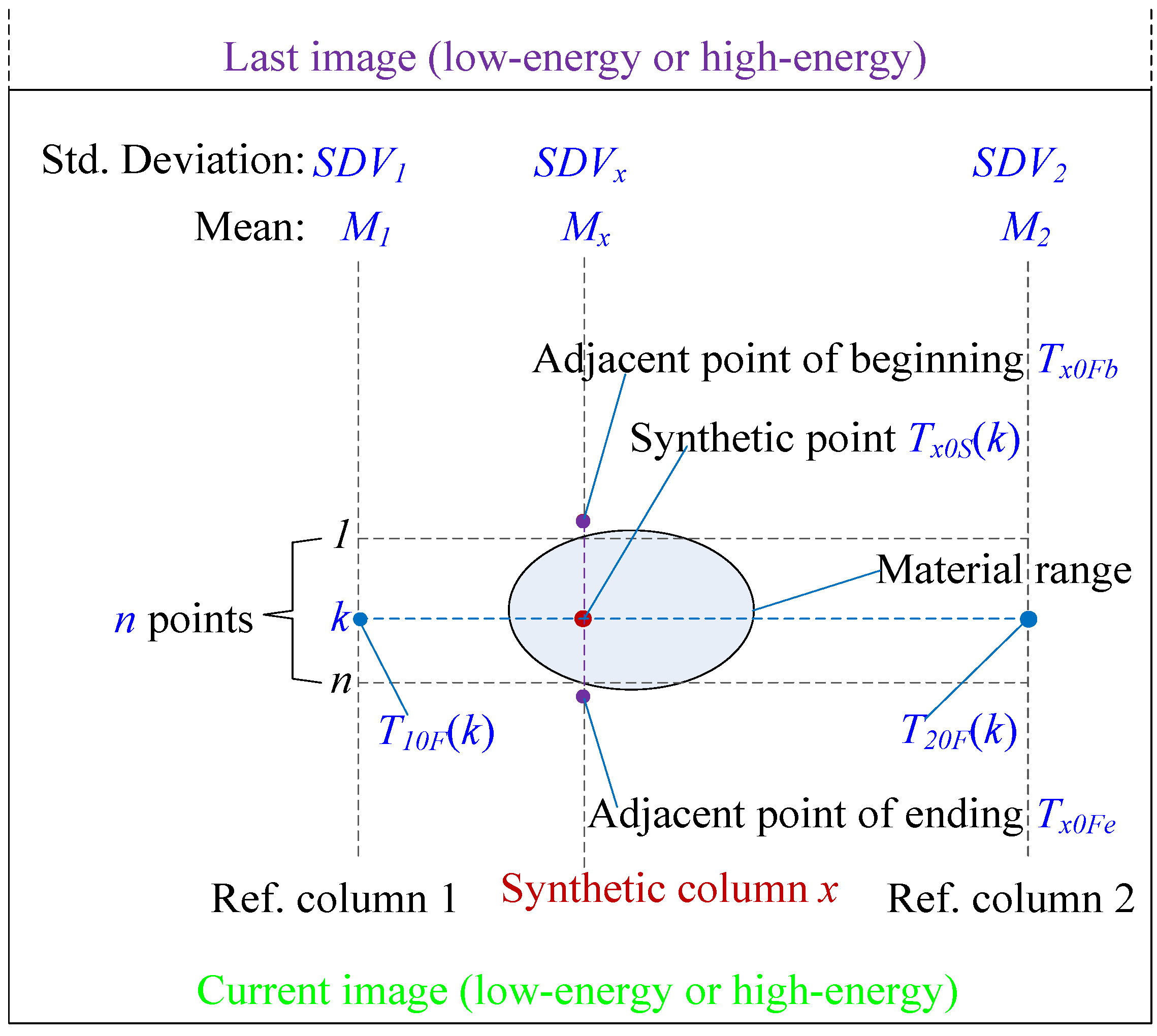
The schematic diagram of synthesis of signals before attenuation within the material range is shown in
Figure 3. The vertical context includes historical statistical data such as the mean and SD of the column where the synthetic curve is located and the signal values of two adjacent points close to the endpoint of the synthetic curve, which have an impact on the mean, fluctuation amplitude and smooth of the endpoint value of the synthetic curve. The horizontal context includes the actual value (after filtering), mean and SD of the current measurable signal without materials in the same time series as the synthetic curve (for example, selecting two columns as reference), which will affect the fluctuation synchronization of the synthetic curve. These are the basic ideas of signal synthesis.
Specifically, it is assumed that the curve requiring synthesis is column x; then it is assumed that the latest statistical data of signals of column x (outside the material range) are SDVx (the SD) and Mx (the mean), that the filtered signal values of the adjacent points at the beginning (upper) and ending (lower) of synthetic curve (column x) is Tx0Fb and Tx0Fe respectively. These data are used as the vertical context. The two reference columns without materials in the current frame of image are selected. Their SDs of the latest statistical data are SDV1 and SDV2, and the means are M1 and M2 respectively. Let the number of signals to be synthesized in column x be n, and the filtered signal point values of the reference columns in the same row as the k-th synthesized signal point in the column x within the material range be T10F(k) and T20F(k). These are used as the horizontal context. The above data can be obtained by statistics of the current and latest data outside the material range, or by filtering the measured values (such as Kalman filtering).
2.2.2. Synthetic method
The deviation value
Ex0S(
k) and signal value
Tx0S(
k) of synthesis of signal before attenuation at a certain column
x and a certain point
k within the range of material to be synthesized are preliminarily calculated as follows:
In Equation (1), the first term is the deviation synthesized according to reference column 1 and the second term is the deviation synthesized according to reference column 2, whose sum with weights of 0.5 and 0.5 is the synthesis deviation Ex0S(k) at point k in the column x synthesis curve.
After the preliminary numerical calculation of the above curve synthetic is completed, the endpoint transition correction is required. The transition correction equation based on the known neighbor values of the endpoints is as follows:
where, the first formula is the beginning-point transition correction, and the second formula is the ending-point transition correction;
τ(
k) is the compensation coefficient. For example, when
k = 1, 2, 3, 4, 5 and
k =
n,
n−1,
n−2,
n−3,
n−4 can be taken respectively,
τ(
k) the corresponding values are 0.875, 0.75, 0.5, 0.25 and 0.125 respectively, which change almost exponentially. It can ensure that the closer the adjacent point to the end of synthetic curve, the greater the impact.
It can be easily extended from the synthetic single column curve to the area array image of the signals before attenuation (within the material range), i.e., the partially mask image synthesis.
2.2.3. Evaluations
The evaluations in this paper need not only curve similarity, but also time synchronization, which is more rigorous than the common ones.
To compare the fluctuation similarity of two time series curves (two columns of the same time series, i.e., the columns of signals in the same row range of the same image), we adopt the Euclidean distance method, and take the ratio of the SD of the distance series corresponding to the two curves to the mean of the two curves as the evaluation, which is called the fluctuation difference of the two curves.
where,
σFC is the fluctuation difference of two curves,
n is the number of curve sequences,
Tij is the signal value of the row
i column
j,
Tik is the signal value of the row
i column
k,
Tij−
Tik (
i=1~
n) is the distance sequence of the two time series curves of column
j and column
k,
μd is the average value of the distance series, and the denominator term of Equation (4) is the total mean value of the two columns of signals compared.
The total degree of coincidence between the synthetic curve and the actual curve is related to the SD and the mean value of the distance between the two. It is measured by the ratio of the root mean square of the distance between the two relatives to 0 and the mean value of the actual curve. It is called the difference of curve synthesis as follows:
where,
σSC is the difference of curve synthesis, which reflects the precision of curve synthesis.
n is the number of synthetic curve sequences,
TiS is the signal value of the row
i of the synthetic curve,
TiR is the signal value of the row
i of the actual curve, and
TiS−
TiR (
i=1~
n) is the directional distance sequence between the synthetic curve and the actual one.
The evaluation equation of the difference of the synthetic image can be extended as follows:
where,
σSS is the difference of surface synthesis,
A is the synthetic surface range,
m is the number of pixel points in
A,
TilS is the signal value in the row
i column
l of the synthetic surface,
TilR is the signal value in the row
i column
l of the actual surface, and
TilS−
TilR (
i,
l∈
A) is the directional distance sequence between the synthetic surface and the actual surface.
The above evaluations are calculated on the basis of the filtered measurable data outside the material as the reference and the synthetic data.
3. Results and Discussion
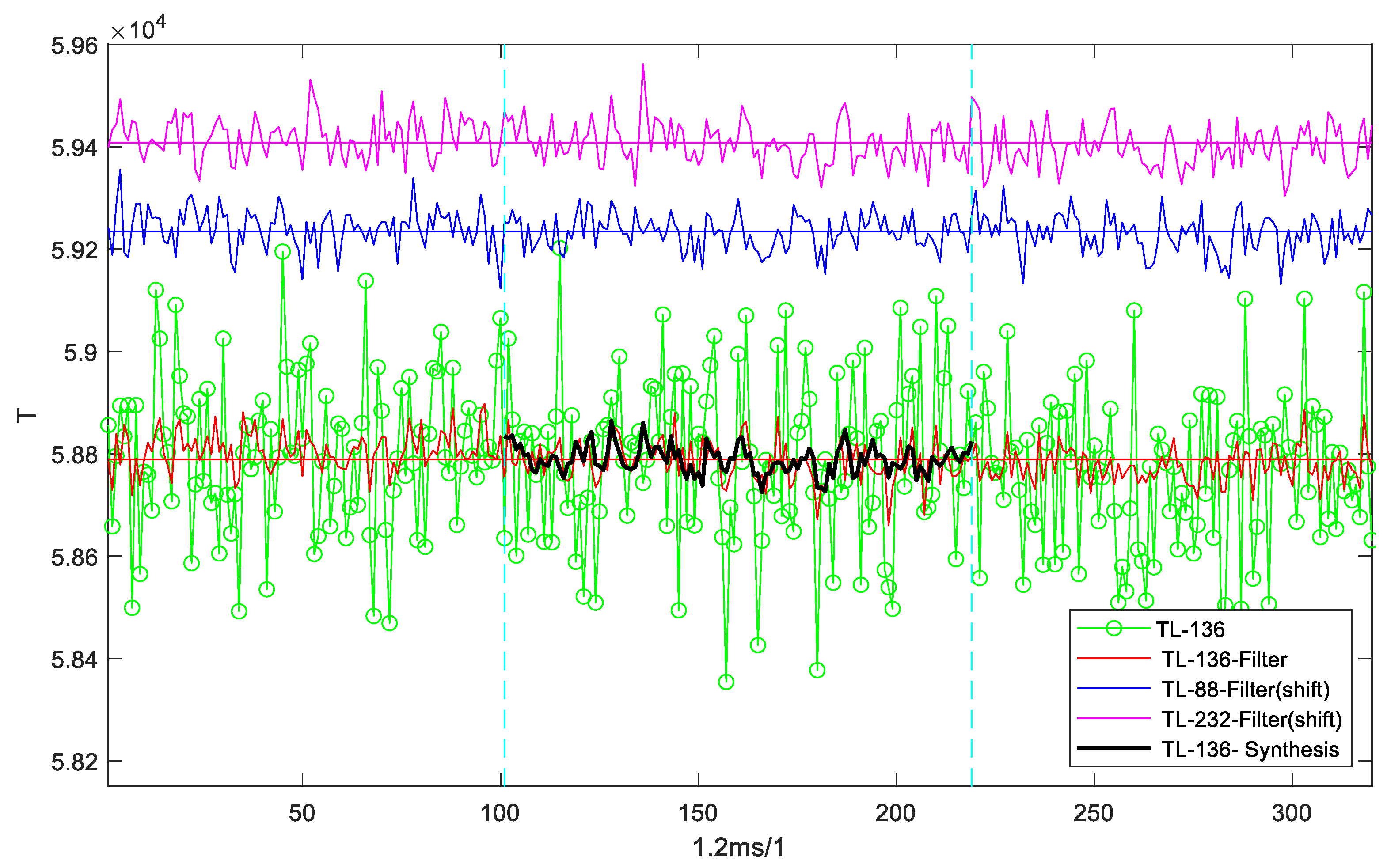
The synthetic curve of signals before attenuation based on the vertical and horizontal bidirectional context is shown in
Figure 4. In the figure, the curve fluctuations in the 88th column (detector channel No. 88, blue, reference column 1), the 232nd column (magenta, reference column 2) and the 136th column (red, synthesis column) original signals after filtering (the improved adaptive Kalman filter [
23] is adopted here) have good synchronization, which also shows that the overall vertical fluctuation of the line-scan detector is synchronous and consistent. Some of the inconsistent fluctuations may be related to the belt thickness change (the belt line is running when data being collected) and occasional noises. The filtered curve (red) in the synthesis column (136th) reflects the low-frequency fluctuation and high-frequency noise filtering effect of the original data (green). The synthetic curve (thick black) is in good agreement with the filtered curve (red) regarded as the true signals. According to Equation (4), the fluctuation difference of the two curves (column 88 and column 232, lines 1-320) is 0.000 959. Compared with the original actual curve of column 136 in the same range, the difference of curve synthesis calculated by Equation (6) is 0.000 661, the fluctuation difference of the two curves (original curve and synthetic curve) is 0.000 662, and PSNR increases by about 1dB, which is better than or basically equivalent to the fluctuation difference of the two reference curves in the actual same image, and shows a pretty good synthetic quality.
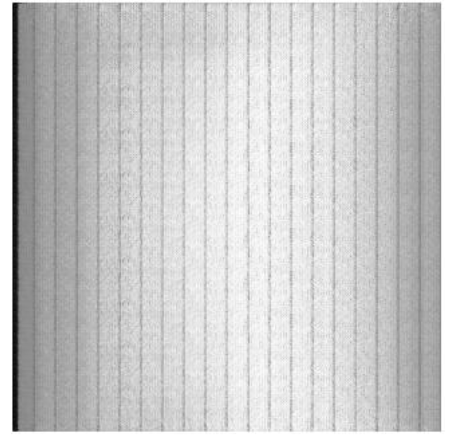
Figure 2a after filtering (improved adaptive Kalman-median filter in Ref. [
23]) is shown in
Figure 5a, and
Figure 2b after filtering and filling the mask part with synthesis surface is shown in
Figure 5b. The difference of surface synthesis between the surface in the green box of
Figure 5b and the surface of the corresponding part of
Figure 5a calculated according to Equation (7) is 0.000 706, which shows that the overall synthetic effect is also quite good. Since the image display is a grayscale image with an intercepted high 8 bits from a 16-bit depth pixel value and the synthesis quality is relatively high, there is almost no difference between the part in the green frame in
Figure 5b and the image in the same area in
Figure 5a by visual inspection. In addition, according to experimental test, the synthetic operation time of the image in
Figure 5b and the corresponding high-energy image is about 35 ms (the SD, mean and synthetic mask image in each column of the low-energy and the high-energy full image are calculated by MATLAB), which is far less than the sampling interval of each frame, i.e., the maximum processing time of 384 ms (the maximum time of total image processing, including filtering, synthesis, identification, control and other operations), accounting for about 9.1%. Moreover, the image synthesis time can be further reduced by hardware acceleration and other measures [
24], so it can meet the real-time requirements.
According to the DCGAN based inpainting method in Ref. [
25], the results after inpainting
Figure 2b are shown in
Figure 6. The comparison with the above vertical and horizontal context synthesis method is shown in
Table 2. Although
Figure 6,
Figure 5b and
Figure 5a are similar in shape, there some large difference between the numerical value of
Figure 6 and the actual original image of
Figure 5a, including that the mean error of a single column (136th) is 3.9%, the PSNR decreases by about 2dB, and the inpainting curve difference is 0.022 and the surface difference is 0.024, which is about 34 times that of the synthetic method; moreover, the training time (4000 training samples) of the model generated by inpainting method is about 2 days, and the inpainting execution time is even more up to 5 days. So, this method may have a good effect on semantic images, but the numerical accuracy is far from the requirements of this paper. Most of the existing image inpainting methods based on deep learning are good at semantic image understanding. Therefore, it can be inferred that the image inpainting methods based on deep learning cannot be directly applied to the high-precision numerical synthesis in this paper, and need to be further researched and improved. What is more, the curve difference and the surface difference by traditional 100-lenth moving average filter are also higher than the deep learning synthetic ones.
For the unmeasurable DE-XRT signals before attenuation
T0 within the range of materials, if the fixed value of one-time acquisition of no material data to obtain the average value is used instead, it cannot well adapt to the impact of slow changes by environment such as temperature, and has a large system error; on the other hand, although the system error can be well overcome and real-time update can be achieved by using the sliding mean outside the material range, it cannot track the low-frequency fluctuation of the actual signal in real-time. Therefore, the signals before attenuation are finely synthesized in this paper, which can match the measurable signals after attenuation that are well filtered. So, it can further improve the calculation accuracy of R_value, lay a good foundation for material identification based on R_value, and have good application value. Although the identification accuracy of subsequent materials is related to different methods, the identification of self-made samples of extended nonferrous metals (Cu, Al, Mg and non-ferromagnetic stainless steel) in our laboratory through the R_value calibration surface nearest neighbor method [
26] shows that the accuracy by count basis was improved from 85% to about 88%, increasing about 3 percentage points. Since the materials must be fully dispersed to facilitate sorting, that is, there is enough space between the materials, so there are many signals for synthesis outside the materials. Therefore, the method in this paper will not lead to the situation that the synthesis effect will be reduced with the increase of the synthesis area in the traditional exemplar-based structure method.
The signal synthesis method in this paper depends heavily on the quality of filtering. It doesn’t work out the problem that the casual noises affect the horizontal synchronization. It is not applicable to the area array image and the high-level semantic incomplete image synthesis. This method can be extended to the fine numerical synthesis or prediction of line-scan incomplete images. Further research on the application of deep learning method to the numerical synthesis of incomplete signals can be carried out.
4. Conclusions
In this paper, a synthesis method based on vertical and horizontal bi-directional context in line-scan DE-XRT signals before attenuation is proposed. The main findings and key innovations are as follows:
1. For the unmeasurable signals before attenuation, according to the vertical and horizontal anisotropy of the line-scan image, the signal synthesis based on different context of vertical and horizontal directions is carried out. The vertical is a time series with continuity of change trend; the horizontal is a spatial characteristic, and there is fluctuation synchronization of signals in the same row.
2. Historical statistical data such as the mean and SD of the signals with a certain time length in the near past in the same column to synthesize and the two reference columns of measurable without material signals, as well as the true value of the reference columns in the same row of the synthesis point, are applied as the synthesis basis of the signal trend and fluctuation amplitude, so that the mean and fluctuation amplitude of the synthesized signals can be accurately updated in real-time.
3. Removing high-frequency noises and retaining the low-frequency fluctuations signals are taken as the reference standard, which is regarded as the real signals.
4. The evaluations of signal synthesis, i.e., the difference of curve synthesis and of surface synthesis, are proposed.
5. The synthesis of non-directly measurable signals before attenuation of line-scan DE-XRT is well realized, which improves the signal numerical precision and the synchronization of high- and low-energy signals, and whose algorithm is simple and can meet the real-time requirements.
The signal synthesis method in this paper can be improved and applied to the signals/image synthesis occasions with line-scan, real-time and high signal numerical precision requirements.
Funding
This research was funded by the Jiangsu Provincial Key Research & Development Program of China, grant number BE2020779.
References
- Jam, J.R.; Kendrick, C.; Walker, K.; et al. A comprehensive review of past and present image inpainting methods. Computer Vision and Image Understanding 2021, 203, 103147. [Google Scholar] [CrossRef]
- Elharrouss, O.; Almaadeed, N.; Al-Maadeed, S.; et al. Image Inpainting: A Review. Neural Processing Letters 2020, 51, 2007–2028. [Google Scholar] [CrossRef]
- Chen, Y.; et al. The improved image inpainting algorithm via encoder and similarity constraint. The Visual Computer 2021, 37, 1691–1705. [Google Scholar] [CrossRef]
- Li, Y.L.; Gao, Y.; Yan, J.L.; et al. Image Inpainting Methods Based on Deep Neural Networks: A Review. Chinese Journal of Computers 2021, 44, 2295–2316. [Google Scholar]
- Qin, Z.; et al. Image inpainting based on deep learning: A review. Displays 2021, 69, 102028. [Google Scholar] [CrossRef]
- Atapour-Abarghouei, A.; Breckon, T.P. A comparative review of plausible hole filling strategies in the context of scene depth image completion. Computers & Graphics 2018, 72, 39–58. [Google Scholar]
- Chen, W.; Li, Y. Recovery of signals under the condition on RIC and ROC via prior support information. arXiv 2016. [Google Scholar] [CrossRef]
- Studer, C.; Kuppinger, P.; Pope, G.; et al. Recovery of sparsely corrupted signals. IEEE Transactions on Information Theory 2012, 58, 3115–3130. [Google Scholar] [CrossRef]
- Wang, L.; Chen, W.; Yang, W.; et al. A state-of-the-art review on image synthesis with generative adversarial networks. IEEE Access 2020, 8, 63514–63537. [Google Scholar] [CrossRef]
- Chen, Y.; Zhao, Y.; Jia, W.; et al. Adversarial-learning-based image-to-image transformation: A survey. Neurocomputing 2020, 411, 468–486. [Google Scholar] [CrossRef]
- Pathak, D.; Krähenbühl, P.; Donahue, J.; et al. Context Encoders: Feature Learning by Inpainting. In IEEE Conference on Computer Vision and Pattern Recognition (CVPR); 2016; pp. 2536–2544. [Google Scholar]
- Song, Y.; et al. Contextual-Based Image Inpainting: Infer, Match, and Translate. In Computer Vision—ECCV 2018; Ferrari, V., Hebert, M., Sminchisescu, C., et al., Eds.; Springer: Cham, 2018. [Google Scholar]
- López-Tapia, S.; Molina, R.; Katsaggelos, A.K. Deep learning approaches to inverse problems in imaging: Past, present and future. Digital Signal Processing 2021, 119, 103285. [Google Scholar] [CrossRef]
- Fang, Y.; Li, Y.; Tu, X.; et al. Face completion with hybrid dilated convolution. Signal Processing: Image Communication 2020, 80, 115664. [Google Scholar] [CrossRef]
- Wang, H.; Jiao, L.; Wu, H.; et al. New inpainting algorithm based on simplified context encoders and multi-scale adversarial network. Procedia Computer Science 2019, 147, 254–263. [Google Scholar] [CrossRef]
- Park, S.W.; Ko, J.S.; Huh, J.-H.; et al. Review on generative adversarial networks: focusing on computer vision and its applications. Electronics 2021, 10, 1216. [Google Scholar] [CrossRef]
- Johnson, D.H. Signal-to-noise ratio. Scholarpedia 2006, 1, 2088. [Google Scholar] [CrossRef]
- Wang, Z.; Bovik, A.C.; Sheikh, H.R.; et al. Image quality assessment: from error visibility to structural similarity. IEEE Transactions on Image Processing 2004, 13, 600–612. [Google Scholar] [CrossRef] [PubMed]
- Cleasby, I.R.; Wakefield, E.D.; Morrissey, B.J.; et al. Using time-series similarity measures to compare animal movement trajectories in ecology. Behavioral Ecology and Sociobiology 2019, 73, 151. [Google Scholar] [CrossRef]
- Geler, Z.; Kurbalija, V.; Radovanović, M.; et al. Comparison of different weighting schemes for the kNN classifier on time-series data. Knowledge and Information Systems 2016, 48, 331–378. [Google Scholar] [CrossRef]
- Efrat, A.; Fan, Q.; Venkatasubramanian, S. Curve matching, time warping, and light fields: New algorithms for computing similarity between curves. Journal of Mathematical Imaging and Vision 2007, 27, 203–216. [Google Scholar] [CrossRef]
- Tao, L.; Lu, C.; Noktehdan, A. Similarity recognition of online data curves based on dynamic spatial time warping for the estimation of lithium-ion battery capacity. Journal of Power Sources 2015, 293, 751–759. [Google Scholar] [CrossRef]
- Xiong, T.; Ye, W. Improved adaptive Kalman-median filter for line-scan X-ray transmission image. Sensors 2022, 22, 4993. [Google Scholar] [CrossRef] [PubMed]
- Xiong, T.; Ye, W. A PC-based control method for high-speed sorting line integrating data reading, image processing, sequence logic control, communication and HMI. AIP Advances 2021, 11, 015123. [Google Scholar] [CrossRef]
- Yeh, R.A.; Chen, C.; Lim, T.Y.; et al. Semantic image inpainting with deep generative models. In IEEE Conference on Computer Vision and Pattern Recognition (CVPR); 2017; pp. 6882–6890. [Google Scholar]
- Xiong, T.; Ye, W.; Xu, X. Combination of dual-energy X-ray transmission and variable gas-ejection for the in-line automatic sorting of many types of scrap in one measurement. Applied Sciences 2021, 11, 4349. [Google Scholar] [CrossRef]
|
Disclaimer/Publisher’s Note: The statements, opinions and data contained in all publications are solely those of the individual author(s) and contributor(s) and not of MDPI and/or the editor(s). MDPI and/or the editor(s) disclaim responsibility for any injury to people or property resulting from any ideas, methods, instructions or products referred to in the content. |
© 2023 by the authors. Licensee MDPI, Basel, Switzerland. This article is an open access article distributed under the terms and conditions of the Creative Commons Attribution (CC BY) license (http://creativecommons.org/licenses/by/4.0/).
