
Submitted:
03 August 2023
Posted:
07 August 2023
Read the latest preprint version here
Abstract
Nearest-neighbour clustering is a simple yet powerful machine learning algorithm that finds natural application in the decoding of signals in classical optical fibre communication systems. Quantum nearest-neighbour clustering promises a speed-up over the classical algorithms, but the current embedding of classical data introduces inaccuracies, insurmountable slowdowns, or undesired effects. This work proposes the generalised inverse stereographic projection into the Bloch sphere as an encoding for quantum distance estimation in k nearest-neighbour clustering, develops an analogous classical counterpart, and benchmarks its accuracy, runtime and convergence. Our proposed algorithm provides an improvement in both the accuracy and the convergence rate of the algorithm. We detail an experimental optic fibre setup as well, from which we collect 64-Quadrature Amplitude Modulation data. This is the dataset upon which the algorithms are benchmarked. Through experiments, we demonstrate the numerous benefits and practicality of using the 'quantum-inspired' stereographic k nearest-neighbour for clustering real-world optical-fibre data. This work also proves that one can achieve a greater advantage by optimising the radius of the inverse stereographic projection.
Keywords:
Quantum K-Means
; Quantum Machine Learning
; Quantum Computing
; K-Means Clustering
; 6G Communication
; Quadrature Amplitude Modulation
; Quantum-Classical Hybrid Algorithms
; Quantum-Inspired Algorithms
1. Introduction
Quantum Machine Learning (QML), using quantum algorithms to learn quantum or classical systems, has attracted a lot of research in recent years, with some algorithms possibly gaining an exponential speedup [1,2,3]. Since machine learning routines often push real-world limits of computing power, an exponential improvement to algorithm speed would allow for such systems with vastly greater capabilities [4]. Google’s ‘Quantum Supremacy’ experiment [5] showed that quantum computers can naturally solve certain problems with complex correlations between inputs that can be incredibly hard for traditional (“classical”) computers. Such a result naturally suggests that machine learning models executed on quantum computers could be more effective for certain applications. It seems quite possible that quantum computing could lead to faster computation, better generalization on less data, or both even, for an appropriately designed learning model. Hence, it is of great interest to discover and model the scenarios in which such a “quantum advantage” could be achieved. A number of such “Quantum Machine Learning” algorithms are detailed in papers such as [2,6,7,8,9]. Many of these methods claim to offer exponential speedups over analogous classical algorithms. However, on the path from theory to technology, some significant gaps exist between theoretical prediction and implementation. These gaps result in unforeseen technological hurdles and sometimes misconceptions, necessitating more careful case-by-case studies.
In this work, we start from a theoretical abstraction of a well-known technical problem in signal processing through optic fibre communication links. Specifically, problems and opportunities are demonstrated for the k nearest-neighbour clustering algorithm when applied to the real-world problem of decoding 64-QAM data provided by Huawei. It is known from the literature that the k nearest-neighbour clustering algorithm can be applied to solve the problem of phase estimation in optical fibres [10,11].
A quantum version of this k nearest-neighbour clustering algorithm has been developed in [2], promising an exponential speedup. However, the practical usefulness of this algorithm is under debate [12]. There are claims that the speedup is reduced to only polynomial once the quantum version of the algorithm takes into account the time taken to prepare the necessary quantum states. This work builds upon several observations.
- In any classical implementation of k nearest-neighbour clustering, it is possible to change the dissimilarity and loss function. This observation carries over to hybrid quantum-classical implementations of k-nearest neighbour algorithms which utilize quantum methods only to estimate the dissimilarity. This is indeed what we do in this work, change to a dissimilarity that is more suitable for quantum embedding.
- The encoding of classical data into quantum states has been proven to be a complex task which significantly reduces the advantage of known quantum machine learning algorithms [12]. Due to this, we focus on (in hindsight) more natural embedding of classical data in quantum states.
In this work, we, therefore, reduce the use of quantum methods to estimate distances and dissimilarities. We thereby minimise the storage time of quantum states by encoding the states before each shot and using destructive measurements. We utilise this process of encoding classical data into quantum states productively by ‘pre-processing’ the data in this step. As in the case of angle embedding, the pre-processing of data before encoding using the unitary is the critical step which we can utilise. We propose an encoding using the inverse stereographic projection (ISP) and show its performance on real-world 64-QAM data. We also introduce an analogous classical quantum-inspired algorithm.
The paper is structured as follows. In the remainder of this introduction, we discuss the related body of work and our contribution to it. In Section 2, we introduce the preliminaries required for understanding our approach and describe the problem to be tackled - clustering of 64-QAM optic fibre transmission data - as well as the experimental setup used. Furthermore, Section 3 introduces the developed stereographic quantum k nearest-neighbour clustering (SQ-kNN). Section 4 defines the developed quantum-inspired 2D Stereographic Classical k Nearest-Neighbour (2DSC-kNN) algorithm and proves its equivalence to the SQ-kNN quantum algorithm. Afterwards, in Section 5, we describe the various experiments for testing the algorithms, present the obtained results, and discuss the conclusions from the experimental results. Section 6 concludes this work and proposes some directions for future research, some of which are partially discussed in the appendix.
1.1. Related Work
A unifying overview of several quantum algorithms is presented in [14] in a tutorial style. An overview targeting data scientists is given in [15]. The idea of using quantum information processing methods to obtain speedups for the k-means algorithm was proposed in [16]. In general, neither the best nor even the fastest method for a given problem and problem size can be uniquely ascribed to either the class of quantum or classical algorithms, as can be seen in the detailed discussion presented in [9]. The advantages of using local (classical) processing units alongside quantum processing units in a distributed fashion are quantified in [17]. The accuracy of (quantum) K-means has been demonstrated experimentally in [18] and in [19], while quantum circuits for loading classical data into a quantum computer are described in [20].
An algorithm is proposed in [2] that solves the problem of clustering N-dimensional vectors to M clusters in time on a quantum computer, which is exponentially faster than time for the (then) best known classical algorithm. The approach detailed in [2] requires querying the QRAM [21] for preparing a ‘mean state’, which is then used to find the inner product between the centroid (by default the mean point) using the SWAP test [22,23,24]. However, there exist some significant caveats to this approach. Firstly, this algorithm achieves an exponential speedup only when comparing the bit-to-bit processing time with the qubit-to-qubit processing time. If one compares the bit-to-bit execution times of both algorithms, the exponential speedup disappears [12,25]. Secondly, since stable enough quantum memories do not exist, a hybrid quantum-classical approach must be used in real-world applications - all the information is stored in classical memories, and the states to be used in the algorithm are prepared in real-time. This process is known as ‘Data Embedding’ since we are embedding the classical data into quantum states. This, as mentioned before [4,25] slows down the algorithm to only a polynomial advantage over classical k-means. However, we propose an approach whereby this step of embedding can be treated as a data preprocessing step, allowing us to achieve an advantage still and make the quantum approach viable. Quantum-inspired algorithms have shown a lot of promise in achieving some types of advantage that are demonstrated by quantum algorithms [4,25,26,27], but as [9] remarks, the massive increase in runtime with rank, condition number, Frobenius norm, and error threshold make the algorithms proposed in [12,25] impractical for matrices arising from real-world applications. This observation is supported by [28].
Recent works such as [25] suggest that even the best QML algorithms, without state preparation assumptions, fail to achieve exponential speedups over their classical counterparts. In [4] it is pointed out that most QML algorithms are incomparable to classical algorithms since they take quantum states as input and output quantum states, and that there is no analogous classical model of computation where one could search for similar classical algorithms. In [4], the idea of matching state preparation assumptions with -norm sampling assumptions (first proposed in [25]) is implemented by introducing a new input model, sample and query access (SQ access). In [4] the Quantum K-Means algorithm described in [2] is ‘de-quantised’ using the ‘toolkit’ developed in [25], i.e. a classical algorithm is given that, with classical SQ access assumptions replacing quantum state preparation assumptions, matches the bounds and runtime of the corresponding quantum algorithm up to polynomial slowdown. From the works [4,25,29], we can conclude that the exponential speedups of many quantum machine learning algorithms that are under consideration arise not from the ‘quantumness’ of the algorithms but instead from strong input assumptions, since the exponential part of the speedups vanish when classical algorithms are given analogous assumptions. In other words, in a wide array of settings, on classical data, these algorithms do not give exponential speedups but rather yield polynomial speedups.
The fundamental aspect that allowed for the exponential speedup in [25] vis-á-vis classical recommendation system algorithms is the type of problem being addressed by recommendation systems in [8]. The philosophy of recommendation algorithms before this breakthrough was to estimate all the possible preferences of a user and then suggest one or more of the most preferred objects. The quantum algorithm promised an exponential speedup but provided a recommendation without estimating all the preferences; namely, it only provided a sample of the most preferred objects. This process of sampling along with state preparation assumptions was, in fact, what gave the quantum algorithm an exponential advantage. The new classical algorithm obtains comparable speedups also by only providing samples rather than solving the whole preference problem. In [4], it is argued that the time taken to create the quantum state should be included for comparison since the time taken is not insignificant; it is also claimed that for every such linear algebraic quantum machine learning algorithm, a polynomially slower classical algorithm can be constructed by using the binary tree data structure described in [25]. Since then, more sampling algorithms have shown that multiple quantum exponential speedups are not due to the quantum algorithms themselves but due to the way data is provided to the algorithms and how the quantum algorithm provides the solutions [4,29,30,31]. Notably, in [31] it is argued that there exist competing classical algorithms for all linear algebra subroutines, and thus for many quantum machine learning algorithms. However, as pointed out in [9] and proven in [28], there exist significant caveats to these aforementioned results of quantum-inspired algorithms. The polynomial factor in these algorithms often contains a very high power of the rank and condition number, making them suitable only for sparse low-rank matrices. Matrices of real-world data are most often quite high in rank and hence unfavourable for such sampling-based quantum-inspired approaches. Whether such sampling algorithms can be used also highly depends on the specific application and whether or not samples of the solution instead of the complete data are suitable. It should be pointed out that in case such complete data is needed, quantum algorithms generally do not provide an advantage anyway.
The method of encoding classical data into quantum states contributes to the complexity and performance of the algorithm. In this work, the use of the ISP is proposed. Others have explored this procedure [32,33,34] as well; however, the motivation, implementation, and use vary significantly, as well as the procedure for embedding data points into quantum states. There has also been no extensive testing of the proposed methods, especially not in an industry context. In our method, we exclusively use pure states from the Bloch sphere since this reduces the complexity of the application. Lemma 3 assures that our method with existing quantum techniques is applicable for nearest neighbour clustering. In contrast, the density matrices of mixed states and the normalised trace distance between the density matrices are used for binary classification in [32,33]. A very important thing to consider here is to distinguish the contribution of the ISP from the quantum effects. We will see in Section 5 that the ISP itself seems to be the most important contributing factor. In [35], it is also proposed to encode classical information into quantum states using the ISP in the context of quantum generative adversarial networks. Their motivation for using the ISP is due to the fact that it is one-one and can hence be used to uniquely represent every point in the 2D plane without any loss of information. Angle embedding, on the other hand, loses all amplitude information due to the normalisation of all points. A method to transform an unknown manifold into an n-sphere using ISP is proposed in [36] - here, however, the property of their concern was the conformality of the projection since subsequent learning is performed upon the surface. In [37], a parallelised version of [2] is developed using the FF-QRAM procedure [38] for amplitude encoding and the ISP to ensure a one-one embedding.
In the method of Spherical Clustering [39], the nearest neighbour algorithm is explored on the basis of the cosine similarity measure (Equation (27) and Lemma 2). The cosine similarity is used in cases of information retrieval, text mining, and data mining to find the similarity between document vectors. It is used in those cases because the cosine similarity has low complexity for sparse vectors since only the non-zero coordinates need to be considered. For our case as well, it is in our interest to study Equations (22) to (24) with the cosine dissimilarity. This, in particular, becomes relevant once we employ stereographic embedding to encode the data points into quantum states.
In this work, we develop an analogous classical algorithm to our proposed quantum algorithm to overcome the many issues faced by quantum algorithms. This work focuses on developing the stereographic quantum and quantum-inspired k nearest-neighbour algorithms and experimentally verifying the viability of the stereographic quantum-inspired k nearest-neighbour classical algorithm on real-world 64-QAM communication data.
1.2. Contribution
The subject of this work is the development and testing of the quantum-analogous classical algorithm for performing k nearest neighbour clustering using the general ISP (Section 4) and the stereographic quantum k nearest-neighbour clustering quantum algorithm (Section 3). The main contributions of this work are (a) the development of a novel quantum embedding using the generalised ISP along with proving that the ideal projection radius is not 1; (b) the development of the 2DSC-kNN classical algorithm through a new method of centroid update which yields significant advantage and; (c) the experimental exploration and verification of the developed algorithms. The extensive testing upon the real-world, experimental QAM dataset (Section 2.1) revealed some very important results regarding the dependence of accuracy, runtime, and convergence performance upon the radius of projection, number of points, noise in the optic fibre, and stopping criterion - described in Section 5. No other work has considered a generalised projection radius for quantum embedding or studied its effect. Through our experimentation, we have verified that there exists an ideal radius greater than 1 for which accuracy performance is maximised. The advantageous implementation of the algorithm upon experimental data shows that our procedure is quite competitive. The fact that the developed quantum algorithm has a completely classical analogue (with comparable time complexity to the classical k means algorithm) is a distinct advantage in terms of in-field deployment, especially compared to [2,9,16,32,33,34,37]. The developed quantum algorithm also has another advantage with respect to Noisy intermediate-scale quantum (NISQ) realisations - it has the least circuit depth and circuit width among all candidates [2,9,34,37] - making it practical to implement with the current quantum technologies. Another important contribution is the our generalisation of the dissimilarity for clustering; instead of Euclidean dissimilarity (distance), we consider other dissimilarities which might be better estimated by quantum circuits (Appendix E). A somewhat similar approach was developed in parallel by [40] in the context of amplitude embedding. All previous approaches [2,9,34,37] only try to estimate the Euclidean distance. We also make the contribution of studying the relative effect of ‘quantumness’ and the ISP, something completely overlooked in previous works. We show that the quantum ‘advantage’ in accuracy performance touted by works such as [32,33,34,37] is in reality quite suspect and achievable through classical means. We describe a generalisation of the stereographic embedding - the Ellipsoidal embedding, which we expect to give even better results.
Other contributions of our work include: the development of a mathematical formalism for the generalisation of the k nearest-neighbour problem to clearly indicate the contribution various parameters such as dissimilarities and dataspace (see Section 2.4) and; presenting the procedure and circuit for stereographic embedding using the angle embedding procedure, which consumes only in time and resources (Section 3.1).
2. Preliminaries
In this section, for completeness, we touch upon some concepts and background information required to understand the paper. This ranges from small general statements on quantum states (Bloch sphere, fidelity and Bell-state measurement in Section 2.2 and Section 2.3) to the basics of k Nearest-Neighbour clustering (Section 2.4, Section 2.5 and Section 2.6) and stereographic projection (Section 2.7). We begin by first describing the optic-fibre experimental setup used for the collection of the 64-QAM dataset, upon which the clustering algorithms were tested and benchmarked.
2.1. Experimental Setup
M-ary Quadrature Ampltiude Modulation (M-QAM) is a simple and popular protocol for digital data transmission through analog communication channels. It is widely used in optic fibre communication networks, and the decoding process of the received data often uses the k Nearest-Neighbour algorithm to cluster nearby points. More details including the description of the model used in the experiments can be found in Appendix A. We now describe the experimental setup used to collect the dataset that is used for testing and benchmarking the clustering algorithms.
The dataset contains a launch-power (laser-power feed into the fiber) sweep (four datasets collected at four different launch powers) of 80 km fibre transmission of coherent dual polarization (DP)-64QAM with a gross data rate of bits/s. For the dataset, we assumed 15% overhead for forward error correction (FEC) and used 3.47% overhead for pilots and training sequences, so the net bit rate is bits/s. Note that the pilots and training sequences are removed after the MIMO equalizer. An overview of the experimental setup [41] to capture this real-world database is shown in Figure 1. Four Samples/s digital-to-analog converters (DACs) generate an electrical signal amplified by four 60 GHz 3dB-Bandwidth amplifiers. A tunable 100 kHz external cavity laser (ECL) source generates a continuous wave signal that is modulated by a 32 GHz DP-I/Q modulator. The receiver consists of an optical 90-hybrid and four 100 GHz balanced photodiodes. The electrical signals are digitized using four 10-bit analog-to-digital converters (ADCs) with Samples/s and 110 GHz. Subsequently, the raw signals are preprocessed by the receiver digital signal processing (DSP) blocks.
The datasets were collected in a very short time, corresponding to the memory size of the oscilloscope, which is limited. This is referred to as offline processing. At the receiver, the signals were normalized to fit the alphabet. The average launch power in watts can be calculated as follows:
There are 4 sets of published data with different launch powers, corresponding to different levels of deterministic nonlinear distortions during transmission: 2.7 dBm, 6.6 dBm, 8.6 dBm, and 10.7 dBm. Each dataset consists of the ‘alphabet’ (initial analog transmission values), the error-corrected received analog values, and the true labels of the transmitted points.
The data has been explained and visualised in detail in the Appendix A.
After obtaining this noisy real-world dataset, our task is to decode the received analog values into bitstrings. The k Nearest-Neighbour algorithm is the candidate of choice since it classifies datasets into clusters by associating an ‘average point’ (centroid) to each cluster. In our method, the objective of the clustering algorithm is first to identify, using the set of received signals, a given number M of centroids (one for each cluster) and then to assign each signal to the ‘nearest’ centroid. The second step is classification. This creates the clusters, which can then be decoded into bit signals through the process of demapping. Demapping consists of mapping the original transmission constellation (alphabet) to the current centroids and then assigning the bitstring label associated with that initial transmission point to all the points in the cluster of that centroid. This process completes the final step of the QAM protocol, translating the analog values to bitstrings read by the receiver. The size M of the constellation is known since we know beforehand which QAM protocol is being used. We also know the “alphabet”, i.e. the initial and ideal points at which the signals were transmitted.
2.2. Bloch Sphere
It is well known that all the qubit pure states can be obtained from the zero state using the unitary U [42]
where
These are unit vectors in the unit sphere of , but it is also well known that the corresponding density matrices are uniquely represented by the Bloch vectors
as points in the unit sphere [42] (the Bloch sphere) through the relation
where is the identity matrix and is the vector of Pauli matrices
Regarding mixed states, notice that Equation (6) is linear and thus convex combinations of density matrices translate to convex combinations of Bloch vectors, meaning that the mixed states are represented by the interior of the sphere. Namely, the most general qubit quantum states can be represented by
Finally, since the Pauli matrices are orthogonal operators under the Hilbert-Schmidt inner product, the fidelity between two quantum states and is easily computed as
Using the Bloch sphere representation of qubit quantum states also makes it easy to find orthogonal states and compute diagonalizations. Indeed, let be a unit vector (), thus representing the pure state , then the orthogonal state to is simply the antipodal point
which can be shown by computing the fidelity as in Equation (8)
Hence, the Bloch eigenvectors for any Bloch vector are simply - the two antipodal points where the line of intersect the Bloch sphere. Namely, for any mixed quantum state corresponding to the Bloch vector , we can decompose the quantum state as
with
In the next section, we discuss how we use the Bell-state measurement to estimate the fidelity between quantum states and exposit when this should be chosen over the SWAP test.
2.3. Bell-state measurement and Fidelity
We use the Bell-state measurement to estimate the fidelity between two pure states. The Bell-state measurement is defined as the von-Neumann measurement of the maximally entangled basis
which by construction is equivalent to a standard basis measurement after as displayed in Figure 2. This measurement can be used to estimate the fidelity as follows.
Lemma 1.
Let and be two qubit pure states and let (the singlet Bell state). Then
Proof.
Let us write the states as
Then the state before the standard-basis measurement is
and in particular the probability of outcome 11 can be written as
The fidelity is obtained now by adding and subtracting and computing
concluding the proof. □
Lemma 1 is used to construct the quantum clustering algorithm in Section 3. We will use the quantum circuit of Figure 2 for fidelity estimation in the developed quantum algorithm.
Remark 1.
Since we are only interested in the outcome and we are measuring qubits, the course-grained projective measurement defined by and is sufficient for the purpose of computing the inner product. The non-destructive version of this measurement is known as the SWAP test [23,24], first described in [22]. This test has been used extensively for overlap estimation in quantum algorithms [2]. The SWAP test requires one to only measure an ancilla qubit instead of the two input qubits, leaving them in the post-measurement state, which can be used later for other purposes. However, given the current limitations of NISQ technologies, storing quantum information for reuse is quite impractical; therefore, we prefer the destructive measurement version for overlap estimation. Namely, we use the Bell-state measurement instead of the SWAP test because the post-measurement state is not needed.
2.4. Nearest-neighbour clustering algorithms
Clustering is a simple, powerful and well-known machine-learning algorithm that has been extensively used throughout the literature. In this section, we summarize some standard and basic notions introduced by clustering and define this class of heuristic algorithms precisely, so that we can make clear the difference between regular clustering and the quantum and quantum-inspired clustering algorithms introduced in this paper. To define the k Nearest-Neighbour Clustering Algorithm, we first define the involved variables.
Definition 1 (Clustering State).
We define ak Nearest-Neighbour Clustering State, or clustering state for short, as a collection where is a space called dataspace and
- is a subset called dataset of points called datapoints
- is a list (of size k) of points called centroids
- is a lower bounded function called dissimilarity function , or dissimilarity for short.
Note that d does not have to be a distance metric. We now define the basic steps that are repeated in the clustering algorithm.
Definition 2 (Clusters and Centroid update).
Let be a clustering state. We define the clusters of the state as, for each , the set
We now define the possible new centroids of a subset as the set
of all points minimizing the total (and thus the average) dissimilarity. Then, we call a centroid update any function (where P denotes the power set) of clusters such that is a possible new centroid, namely such that , for all . We then define the following short-hand notation for the centroid update of , namely the new list of centroids
We now define the general k nearest-neighbour clustering algorithm.
Definition 3 (K-Nearest-Neighbour Clustering Algorithm (kNN)).
Finally, we define a K-Nearest-Neighbour clustering algorithm (kNN) as a pair of clustering state and centroid update . The kNN algorithm defines a sequence of clustering states via for all which we call the iterations (of the algorithm).
A point of note is that Equation (23) implies that the new centroid is one of the points in the dataspace that minimizes the total (and hence the average) dissimilarity with all the points in the cluster. Also notice that this definition requires one to initialise or populate the list with initial values, i.e. the initial centroids must be defined as a starting point for the clustering algorithm. The initial centroids can either be assigned randomly or defined as a function of parameters such as the dataset.
Another comment about Equation (23): in our case, we will see later in Section 3.2 that all choices of points from the set will be equivalent. As in our algorithm, this freedom of choice can be exploited to reduce the amount of computation or for other optimisations.
Notice that Equation (23) and (24) implies that centroids are generally not part of the original data set; however, according to Equation (23) and (24) they must be restricted to the space in which the dataset is defined. Definitions involving centroids for which are possible, but are not used in this work.
One can see that any k nearest-neighbour clustering algorithm can be broken down into 2 steps that keep alternating until a stopping condition (a condition which when true forces the algorithm to terminate) is met: a cluster update which updates the points associated with the newly calculated centroid, and then a centroid update which recalculates the centroid based upon the new points associated to it through its cluster. For the cluster update, the value of the centroid calculated in the previous iteration is taken, and its cluster set is constructed by collecting all the points in the dataset that are ‘closer’ to it than any other centroid. The ‘closeness’ is computed by using a pre-defined dissimilarity. In the next step, the centroids are updated by searching in the dataspace, for each updated cluster, a new point for which the sum of dissimilarities between that point and all points in the cluster is minimised.
It can also be seen that this procedure will lead to different results if one changes the dissimilarity and/or the space of data points. In this paper, we explore the effects of changing this dissimilarity as well as the space of data points, and we shall explain it in the context of quantum states.
2.5. Euclidean dissimilarity and classical clustering
It can be seen from the centroid update in Equation (22) and (23) that the dissimilarity plays a central role in the clustering algorithm. The nature of this function directly controls the first step of cluster update since the dissimilarity is what is used to compute the ‘closeness’ between any two points in the dataspace. It is also very clear that if in the centroid update, the dissimilarity is changed, the points at which the minimum is achieved could also change.
The Euclidean dissimilarity is defined simply as the square of the Euclidean distance between the points:
For a finite subset , the minimization of Equations (23) and (24) yields a unique point, reducing to the average point of the cluster:
which we call the Euclidean centroid update. This is the most typical case of centroid update where the new centroid is updated as the mean point of all points in the cluster. This corresponds to the classic k-means clustering algorithm [43], which now can be defined as follows.
Definition 4 (n-Dimensional Euclidean Classical kNN (nDEC-kNN)).
An n-dimensional classical Euclidean kNN algorithm is any clustering algorithm with dataspace , Euclidean dissimilarity and cluster update as the average point, as in Equation (26). Namely, any clustering algorithm of the form .
The computation of the centroid through Equation (26) instead of Equations (23) and (24) reduces the complexity of the centroid update step; such a reduced expression is used to compute the updated centroids rather than searching the entire dataspace for the minimising points during the centroid update.
2.6. Cosine dissimilarity
In this work, we project the collected two-dimensional dataset (described in Section 2.1) into a sphere via the ISP. After this projection, the calculation of the centroids according to Equation (26) would generally yield centroids which lie inside the sphere instead of on the surface due to the convex nature of the sphere’s surface.
In our work, in order to use qubit pure states, we restrict the dataspace to the sphere surface , forcing the centroids to lie on the surface of a sphere. This naturally leads to the question of what the proper reformulation of Equations (23) and (24) is, and whether a computationally inexpensive formula similar to Equation (26) exists for this case as well. This question will be answered in Lemma 3. For this purpose, it is useful to first define the cosine dissimilarity [44] and see how it relates to the Euclidean dissimilarity.
Definition 5 (Cosine Dissimilarity).
For two points, and in an inner-product space the cosine dissimilarity is defined as:
where is the inner product between the 2 points expressed as vectors from the origin, is the norm of induced by the inner product.
This is called cosine dissimilarity because when the cosine dissimilarity reduces to , where is the angle between and . The cosine dissimilarity is also known sometimes as cosine distance (although it is not a distance), while is well known as cosine similarity. This quantity, by construction, only depends on the direction of the vectors and not their magnitude. Said otherwise we have
for any positive constant . We also note that cosine dissimilarity of Equation (27) can be related to the Euclidean dissimilarity of Equation (25) if and lie on the n-sphere of radius r, as stated by the following lemma.
Lemma 2.
Let and be the cosine and Euclidean dissimilarities, respectively. Let , be points on the n-sphere of radius r, then
Proof.
Assuming , , Equation (27) reduces to:
then
concluding the proof. □
From this, we can already expect that the minimizer of the centroid update equation (Equation (23)) computed using the cosine dissimilarity will have a close relation to the Euclidean centroid update. However, the derivation is not so straightforward since the Euclidean centroid update does not lie on the same sphere, but lies inside at a smaller radial distance. This is shown in the following lemma.
Lemma 3.
Let be a finite set, then
We call this the cosine or spherical centroid update. In particular, thus
where is the Euclidean centroid update of Equation (26).
Proof.
The second claim is trivial, we thus have to prove only the first claim. Given that , then according to Lemma 2, the cosine dissimilarity given in Equation (27) reduces for all to:
The minimization in Equation (23) can then be calculated for the cosine dissimilarity with a Lagrangian (see Equation (37)) that satisfies Equation (23) and Equation (24) at the minimizing point. Namely, we have to find that minimises
subject to the restriction condition that assures that , that is
Such a Lagrangian is expressed as
where is the Lagrangian multiplier. We then proceed to calculate the centroid update by employing the derivative criteria to Equation (37).
Therefore the following holds:
Substituting Equation (39) into the restriction in Equation (36), we obtain the multiplier as:
Therefore, the critical point and minimising point is written as
as claimed. □
We can observe that Lemma 3 implies that the minimizer obtained by restricting the point to lie on the surface of the sphere is the projection (from the origin) of the minimizer of the Euclidean dissimilarity into the sphere’s surface.
Corollary 1.
Let be a finite set, the possible new centroids of C under cosine dissimilarity in are
We call these the cosine possible new centroids.
Proof.
We have
where the last equality follows from Equation (28), namely
for all r and ; thus making all the points , equivalent possibilities for the centroid update. □
2.7. Stereographic projection
The inverse stereographic projection (ISP), shown in Figure 3, is a bijective map
from the Euclidean space into an n-sphere without the north pole N.
The reason why this map is interesting is due to the natural equivalence between the 3D unit sphere and the Bloch sphere of qubit quantum states. In this case, as displyed in Figure 3, the ISP maps a 2-dimensional point into a three-dimensional point through the following set of transformations:
The polar and azimuthal angles of the projected point are given by the expressions:
This information, particularly Equation (51), will allow us to associate each point in to a unique quantum state through the Bloch sphere. Still, the inverse stereographic projection does not need to be bound to the preparation of quantum states and can be used as a transformation between classical kNN algorithms. Indeed, we can stereographically project and then perform classical clustering on the 3D data, namely perform 3DEC-kNN as defined in Definition 4. This produces the following algorithm.
Definition°6°(3D°Stereographic°Classical°kNN°(3DSC-kNN)).
Let be an ISP, and let be a clustering state (recall, D is the dataset and are the initial centroids). We then define the 3D Stereographic Classical kNN (3DSC-kNN) as (, , , .
Here we apply elementwise and thus for any list of centroids and for any set of points C, and where are the clusters as defined in Equation (22).
Remark 2.
Derivations and further observations can be found in Appendix C. Of particular note, as explained in more detail in Appendix C.2, is the fact that changing the distance of the plane from the centre of the sphere is equivalent to a change of radius. Therefore we can limit our analysis to projections where the centre of the plane is also the centre of the sphere without loss of generality.
3. Stereographic Quantum Nearest-Neighbour Clustering (SQ-kNN)
In this section, we propose and describe the quantum k (nearest-neighbour) clustering using the stereographic embedding. We demonstrate an equivalent quantum-inspired (classical) version of it in the next section, Section 4. In the Section 3.1 next, we define the method to convert the classical data into quantum states. In what follows, we describe how these states are manipulated so that we obtain an output that can be used to perform clustering. In Section 2.3, we show how the circuit of Section 2.3 can be used for dissimilarity estimation. Section 3.2 defines the quantum algorithm in terms of Definitions 1 to 3, and Section 3.3 discusses the complexity and scalability of the algorithm.
3.1. Stereographic Embedding, Bloch Embedding and Quantum Dissimilarity
For quantum algorithms to work on classical data, the classical data must be converted into quantum states. This process of encoding classical data into quantum states is also called embedding. The process of embedding classical data into quantum states is not unique, and the pros and cons of each technique have to be weighted in the context of a specific application. The process of data embedding is an active field of research, more details on existing embedding can be found in Appendix B.
Here, we propose the stereographic embedding as an improved embedding of classical vector into quantum state using the stereographic projection. We can split stereographic embedding into two steps: inverse stereographic projection and Bloch embedding. We define Bloch embedding, a variation of angle embedding, as follows.
Definition 7 (Bloch embedding).
Let . We define the Bloch embedded quantum state , or Bloch embedding for short, of as the quantum state
which is simply the pure state obtained using as Bloch vector.
To actually obtain the state can be encoded as explained in the preliminaries in Section 2.2, through Equations (2) and (6). For Bloch embedding, the and of Equations (2) and (6) would be the polar and azimuthal angles of respectively. We now define the quantum dissimilarity as follows.
Definition 8 (Quantum Dissimilarity).
For any 2 points , we define the quantum dissimilarity as
where is the Bloch embedding of .
Notice that as per this definition, the classical 2-dimensional points are embedded in pure states only. In Section 3.4, we consider Bloch embedding the centroids also into mixed states and show that it does not give an advantage in our framework. This quantum dissimilarity can be obtained either with the SWAP test or with the Bell state measurement on as described in Section 2.3. In our application, we use the Bell state measurement (depicted in Figure 2)), as we do not need the extra resources of the SWAP test that allow to keep the post-measurement state. For more details, see Lemma 1.
By Equation (8), the quantum dissimilarity is proportional to the cosine dissimilarity1
It is also proportional to the Euclidean distance for points lying on the same sphere (points with the same magnitude) as per Lemma 2. Namely, if then:
We can finally define stereographic embedding as follows
Definition 9 (Stereographic Embedding).
The stereographic embedding of a classical vector consists of
- 1.
- projecting the 2D point into a point on the sphere of radius r in 3D space through the ISP:
- 2.
- Bloch embedding into .
A very time-consuming computational step of the k nearest-neighbour algorithm involves the repeated calculations of distances between the data set points meant to be classified and each centroid. In the case of the quantum k nearest-neighbour algorithm in [2], since angle embedding is not one-one, many steps must be spent after the estimation of the fidelity to calculate the actual distance between the points using the norms. Even in [32,33,37], the norms of the points have to be stored classically and this leads to much computational expense. Our method has the clear benefit of calculating the cosine dissimilarity directly through fidelity estimation. No further calculations are required due to all stereographically projected points having the same norm r in the sphere, and the existence of a bijection between the ISP and the original 2D datapoints, thus saving computational time and resources. In summary, Equations (54) and (55) portray a method to measure a dissimilarity that leads to consistent clustering involving pure states.
As one can see, in the case of stereographically projected points, is directly proportional to the Euclidean dissimilarity between them. Since all the points after projection into the sphere have equal modulus r, and each projected point corresponds to a unique 2D data point, we can directly compare the probability of getting a 11 on the Bell-state measurement circuit for cluster assignment. This eliminates extra steps needed during computation to account for the different moduli of points on the 2-dimensional plane.
3.2. The SQ-kNN Algorithm
We now have all the building blocks needed to define the quantum clustering algorithm. The quantum part will be the dissimilarity estimation , obtained by embedding the data into quantum states as described in Section 3.1 and then feeding it into the quantum circuit described in Section 2.3 and Figure 2 to estimate an outcome probability. The finer details of distance estimation are further described in Appendix E. We can now formally define the developed algorithm building on the definition of clustering state (Definition 1), of clustering algorithm and cluster update provided by Definitions 2 and 3, of ISP as defined in Section 2.7 and of quantum dissimilarity from Definition 8.
Definition 10 (Stereographic Quantum kNN (SQ-kNN)).
Let be the ISP, let be the quantum dissimilarity and let be a clustering state (where D and are 2-dimensional dataset and initial centroids). We then define the Stereographic Quantum kNN (SQ-kNN) as the kNN clustering algorithm
where .
The complete process of performing SQ-kNN in practice can be described in detail as follows.
- 1.
- First, prepare to embed the classical data and initial centroids into quantum states using the ISP: project the 2-dimensional datapoints and initial centroids (in our case, the alphabet) into a sphere of radius r and calculate the polar and azimuthal angles of the points. This first step is executed entirely on a classical computer.
- 2.
- Cluster Update: The calculated angles are used to create the states using Bloch embedding (Definition 7). The dissimilarity between the centroid and point is then estimated by using the Bell-state measurement. Once the dissimilarities between a point and all the centroids have been obtained, the point is assigned to the cluster of the ‘closest’ centroid. This is repeated for all the points that have to be classified. This step is entirely handled by the quantum circuit and classical controller. The controller feeds in the classical values at the appropriate times, stores the results of the various shots and classifies the point to the appropriate cluster.
- 3.
- Centroid Update: Since any non-zero point on the subspace of (see Corollary 1, Figure 4) is an equivalent choice, to minimise computational expense, the centroids are updated as the sum point of all points in the cluster - as opposed to the average, for example, which minimizes the Euclidean dissimilarity (Equation (26)).
Once the centroids are updated, Step 2 (Cluster Update) is repeated, followed once again by Step 3 (Centroid Update) until a decided stopping condition is fulfilled.
Compared to 2D quantum kNN clustering with angle or amplitude embedding, the differences with the SQ-kNN algorithm lie in the embedding and in the postprocessing after the inner-product estimation.
-
The stereographic embedding of the 2D datapoints is done by inverse stereographic projecting the point into a sphere of a chosen radius and then producing the quantum state obtained by rescaling the sphere to radius one.In contrast, in angle embedding, the coefficients of the vectors are used as the angles of the Bloch vector (also known as dense angle embedding [46]), while in amplitude embedding they are used as the amplitudes in the standard basis. For 2D vectors, amplitude embedding allows one to encode only one coefficient (instead of two) in one qubit, and sometimes angle embedding would also encode only one coefficient by using a single rotation (standard angle embedding [47]). Both angle and amplitude embeddings require the lengths of the vectors to be stored classically beside the quantum state, which is not needed in Bloch embedding.
- No post-processing is needed after the overlap estimation of stereographically embedded data as the obtained estimate is already a linear function of the inner product, as opposed to standard approaches using angle or amplitude encoding. Amplitude embedding also requires non-trivial computational time in the state preparation process. In contrast, in angle embedding, though the state preparation time is constant, the process of recovering a useful dissimilarity (e.g. Euclidean) may involve many post-processing steps.
In short, stereographic embedding has the advantage of angle over amplitude embedding of being able to encode all values of a vector and low state preparation time, and the advantage of amplitude versus angle embedding in the recovery of the dissimilarity.
3.3. Complexity Analysis and Scaling
Let the ISP of a d-dimensional point into , using the point (the ‘North pole’) as the projection point, be the point . It is known that the Cartesian co-ordinates of are given by:
where . Hence one can see that the time complexity of projection for a single dimensional point is , provided we only need the Cartesian co-ordinates. However, for the Stereographic Embedding procedure, one would need to calculate the angles made by with the axes of the space, making the time complexity of projection . Therefore, the total time complexity of the Stereographic Embedding for a dimensional dataset and set of initial centroids is given by . We now specify 2 strategies for scaling our algorithm for higher dimensional datapoints.
3.3.1. Using qubit-based system
If we have a qubit-based system, and we use dense angle encoding for encoding the stereographically projected point, we would encode the d calculated angles using qubits. Namely, for the -dimensional projection of a d-dimensional point , one would get d angles that specify the projected point on . We then encode this vector using the same unitary as follows:
If d is odd we can pad with an extra 0 to make it even. Let another point be encoded into the state
Now, to find the overlap between the states, one would have to perform the Bell-state measurement (Section 2.3) pairwise using and as inputs, i.e.
The quantum dissimilarity would then be
This implies that the time complexity of distance estimation would be as the time complexity of the unitary for embedding is still . In the common practical case of the vectors being expressed in an orthogonal basis, we would only have to find the overlap for . We would then have the quantum dissimilarity as
which follows from Equation (55). This would lead to a time complexity of . An important point to note is that with the strategy of pairwise overlap estimation is that if the number of shots to estimate is kept constant, the error in estimation will be for the case of non-orthogonal basis vectors and in the case of orthogonal basis vectors. Hence, taking into account the increase in the number of shots to estimate the overlap with a given total error , the time complexity of this qubit implementation of overlap estimation between two points using SQ-kNN scales as . Hence for all points and clusters the time complexity would be .
It is shown in [48] that for overlap estimation collective measurements are a better strategy than repeated individual measurements. Although this is shown in [48] for the estimation of overlap between 2 states given the availability of multiple copies of the same states, similar collective measurement strategies could be applied in this case for better results. In conclusion, the time complexity of SQ-kNN for qubit-based implementation is
3.3.2. Using qudit-based system
Consider
Then for any two real vectors and , namely when we have
Now, if we make a qudit Bell measurement2, one of the basis state of this von Neumann measurement will actually be
Thus, the inner product between two real vectors can still be measured with a Bell measurement but the resulting probability of measuring outcome scales as
meaning that, as the inner product remains constant going to higher dimension, the number of shots needed to estimate the inner product with constant precision scales polynomially in the dimension. In contrast, such complexity for the swap test remains constant because the contribution of the fidelity to the outcome probability is not divided by the dimension d. This is why the swap test is usually considered for inner product estimation, even if in the case of qubits the Bell measurement is a simpler solution [49].
3.4. SQ-kNN and Mixed states
Instead of estimating the quantum dissimilarity, we can use the datapoints produced by the ISP to perform classical kNN clustering on the 3D projected data. We called this the 3DSC-kNN (3D Stereographic Classical kNN) in Definition 6. This algorithm produces centroids that are inside the sphere. That is, as previously pointed out, when computing the Euclidean 3D centroid on the data projected on the sphere, the result is a point inside the sphere rather than on the sphere itself.
In the Bloch sphere, internal points are mixed states, namely states with added noise. In contrast, the quantum algorithm (SQ-kNN), always produces pure centroids, namely points on the boundary of the sphere. The only noiseless states are the pure states on the boundary of the sphere, and thus the intuition is arguably that mixed states should not help. However, this is not immediately clear from the algorithm. Comparing 3DEC-kNN to SQ-kNN, it is thus natural to ask whether embedding the centroids into mixed states inside the Bloch sphere improves the accuracy.
Here, we show that the intuition is correct, namely that projecting into the pure state centroid is a better option. The reason is that, while the quantum dissimilarity is proportional to the Euclidean dissimilarity for states in the same sphere, the same is not true for Bloch vectors with different lengths.
To allow for mixed state embedding, we can modify the definition of quantum dissimilarity (Equation (55)) to produce mixed states whenever the 3D vector has a length of less than one. This results in the following new quantum dissimilarity.
Definition 11 (Noisy Quantum Dissimilarity).
Let be the ball of radius 1. We define the noisy quantum dissimilarity as the function
where is the quantum state of the Bloch vector as in Equation (7).
Now suppose we have a convex combination of pure states; namely, suppose we have
where is a probability distribution ( and ). By linearity we have
By convexity, will always lie in the sphere. Namely, we have and thus by linearity
The result in Equation (67) can be interpreted as another two step process: first, repeatedly performing the Bell-state measurement of each state that makes up the cluster and corresponding to the datapoint, to estimate each individual dissimilarity; and then, taking the weighted average of the dissimilarities according to the composition of the mixed state centroid. This procedure is clearly impractical experimentally and no longer correlates to the cosine dissimilarity for mixed states.
Computing the diagonalization of as per Equation (11)
(where is the Bloch embedding) makes the estimation more practical by reducing it to two estimations of , namely
The implementation portrayed at Equation (71) simplifies the measurement procedure of the mixed state. Furthermore, instead of estimating separately, the estimation can be done directly by preparing with probability p and with probability , and finally collecting all the outcomes in a single estimation, which simply requires a larger number of shots to achieve the same precision of estimation. Another issue is that the points have to be computed which is quite time-consuming. This is true even for Equation (67); however, a number of shots proportional to the number of Bloch vectors in the cluster is needed for an accurate estimation. Regardless, linearity and convexity make it clear that using mixed states can only increase the quantum dissimilarity.
Namely, while in Euclidean dissimilarity points inside the sphere can reduce the dissimilarity, the quantum dissimilarity is proportional to the Euclidean dissimilarity only for unit vectors, and actually increases for points inside the Bloch sphere. Hence we conclude that the behaviour of 3DSC-kNN does not carry over to SQ-kNN.
4. Quantum-Inspired Stereographic K Nearest-Neighbour Clustering
Through the previous section, Section 3, we have detailed the developed quantum algorithm. In this section, we develop the classical analogue to this quantum algorithm - the ‘quantum-inspired’ classical algorithm. A table summarizing all the algorithms discussed in this paper, including the next one, can be found in Table 1. We begin by defining this analogous classical algorithm in terms of the clustering state (Definition 1), deriving a relationship between the Euclidean and spherical centroids given datapoints that lie on a sphere, and then proving our claim that the defined classical algorithm and previously described Stereographic Quantum K Nearest-Neighbour Clustering algorithms are indeed equivalent.
Recall from Lemma 3 that
Definition 12 (2D Stereographic Classical kNN (2DSC-kNN)).
Let be the ISP, and let be a 2D euclidean clustering state. We define the 2D Stereographic Classical kNN (2DSC-kNN) as
Remark 3.
Notice that due to the cluster update being cosine () and Lemma 3, we can equivalently substitute with , namely we can substitute it without changing the outcome of the cluster update. In our implementation, for simplicity of coding, we indeed used the Euclidean dissimilarity.
To expand upon Definition 12, for the quantum-inspired/classical analogue stereographic k nearest-neighbour clustering algorithm, the steps of execution are as follows:
- 1.
- Stereographically project all the 2-dimensional data and initial centroids into the sphere of radius r. Notice that the initial centroids will lie on the sphere by construction.
- 2.
- Cluster Update: Form the clusters using the method defined in Equation (22), i.e. form all . Here, and dissimilarity (Definition 5 and Lemma 2).
- 3.
- Centroid Update: A closed-form expression for the centroid update was calculated in Equation (41) . This expression recalculates the centroid once the new clusters have been formed. Once all the centroids are updated, Step 2 (cluster update) is then repeated, and so on, until a stopping condition is met.
4.1. Equivalence
We now want to show that the 2DSC-kNN algorithm of Definition 12 is equivalent to the previously defined quantum algorithm using stereographic embedding (Definition 10). For that, we first define what the equivalence of 2 clustering algorithms means.
Definition 13 (Equivalence of Clustering Algorithms).
Let and be two clustering algorithms. They are said to be equivalent if there exists a transformation such that it maps the data, initial centroids and centroid update, and clusters of to the data, initial centroids and centroid update, and clusters of ; namely if
- 1.
- ,
- 2.
- and ,
- 3.
- for all and any .
where we apply t elementwise and thus for any list of centroids and for any set of datapoints C, and where are the clusters as defined in Equation (22).
Theorem 1.
SQ-kNN (Equation 10) and 2DSC-kNN (Equation 12) are equivalent.
Proof.
By definition, let be the 2D clustering state and thus giving us the SQ-kNN algorithm as
and the 2DSC-kNN clustering algorithm as
where
Let us use the notation and define the transform as , which rescales any vector to have length r. Observe that trivially for all , and thus . Therefore
Also the equivalence of centroids is obtained since
For the clusters, we prove the equivalence of the cluster updates as follows. We will use (Equation (54)) and the fact that and are invariant under t, namely and , or more explicitly
Let now . Then, using the above equations and that , we have
where the change in the dissimilarity inequality has also transformed the calculation of into the calculation of . We are now done, since for and thus
This concludes the proof □
The following discussion provides a visual intuition of Theorem 1. In Figure 4, the sphere with centre origin (O) and radius r is the stereographic sphere into which the 2-dimensional points are projected, while the sphere with centre O and radius 1 is the Bloch sphere. The points are the stereographically projected points defining a cluster, corresponding to the previously used labels . The centroid is obtained with the euclidean average in . In contrast, the centroid is restricted to be in and equal rescaled to lie on this sphere. The quantum states are obtained after Bloch embedding the stereographically projected points , and is the quantum state obtained after Bloch embedding the centroid. The points marked on the Bloch sphere in Figure 4 are the Bloch vectors of the quantum states and .
One can see from Definition 7 that the origin, any point on the sphere and are collinear. Hence, it can be seen that in the process of SQ-kNN clustering, the points on the stereographic sphere are projected radially into the sphere of radius 1. Once the labels were assigned in the previous iteration, the new centroid is computed, giving an integer multiple of the average point , which lies within the stereographic sphere. Crucially, when we embed this new centroid into the quantum state for the quantum dissimilarity calculation of the next step, since we only use the polar and azimuthal angle of the point for embedding (see Definition 7), the prepared quantum state is also projected into the surface of the Bloch sphere - or, in other words, a pure state is prepared (). Hence, we can see that all the dissimilarity calculations in the quantum k nearest-neighbour algorithm will take place between points on the surface of the Bloch sphere, even though the calculated quantum centroid is contained outside the stereographic sphere. This argument also illustrates why any point on the ray can be used for the centroid update step of the stereographic quantum k nearest-neighbour clustering algorithm; any chosen point on the ray, when embedded into a quantum state for dissimilarity calculations will reduce to .
In short, we know from Lemma 3 that and lie on a straight line. Therefore one can see that if the Bloch sphere is scaled by r, the point on the Bloch sphere corresponding to will transform to , i.e. and are all collinear. Equation (55) shows that SQ-kNN clustering clusters points on a sphere as per Euclidean dissimilarity; that implies that simply scaling the sphere makes no difference to the clustering. Therefore, we conclude that clustering on the surface of the stereographic sphere with Euclidean dissimilarity is exactly equivalent to quantum k nearest-neighbour clustering with stereographic embedding.
4.2. Complexity Analysis and Scaling
As we showed in Section 3.2, the time complexity of ISP for calculating Cartesian co-ordinates of a dimensional vector is . Hence the total time complexity of projection for the 2DSC-kNN will be where is the total number of points and k is the total number of centroids. Since the cluster update step uses Euclidean dissimilarity, it will take time in total ( for each distance calculation, to be done for each pair of N points and k centroids). The centroid update expression (Equation (41)) can be calculated in making the total time for this step since we have k centroids. Hence we have
on par with the classical k-means clustering algorithm, and at least polynomially faster than the Stereographic Quantum K Nearest-Neighbour Clustering algorithm (Equation (63)) or Lloyd’s quantum clustering algorithm (taking into account input assumptions) [2,9,12].
5. Experiments and Results
We defined the procedure for performing quantum k nearest-neighbour clustering using stereographic embedding in Section 3. Section 3.1 introduces our idea for state preparation - projecting the 2-dimensional data points into a higher dimension. Section 3.1 details the hybrid quantum-classical method used for our process and then proves that the output of the quantum circuit is not only a valid but also an excellent metric that can be used for distance estimation between 2 points. Section 4 describes the quantum-inspired classical algorithm that is analogous to the quantum algorithm. In this section, we test and compare the quantum-inspired rather the quantum algorithm for two main reasons:
- The hardware performance and availability of quantum computers (NISQ devices) is currently so much worse than that of classical computers that most likely no advantage can be obtained with the quantum algorithm.
- The goal of this paper is not to show a “quantum advantage” over the classical k-means in the NISQ context - it is to show that stereographic projection can both lead to better learning for classical clustering and be a better embedding for quantum clustering. In particular, the equivalence between 2DSC-KNN and SQ-KNN proves that the only limitation for the stereographic quantum algorithm to achieve the performance of the quantum-inspired algorithm is noise.
All the experiments were carried out on a server with the following specifications: 2 Intel Xeon E5-2687W v4 chips clocked at 3.0 GHz (24 cores / 48 threads), 128GB RAM. All experiments are performed on the real-world 64-QAM data provided by Huawei (see Section 2.1 and Appendix A). Due to the extensive nature of testing and the large volume of analysis generated, we do not present all the figures in the following sections. Figures which sufficiently demonstrate general trends and observations have been included here. An exhaustive collection of all figures and other such analysis results, as well as the source code, real-world data, and raw data collected, can be obtained from the GitHub repository of the project.
The terminology used is as follows:
- 1.
- Radius: the radius of the stereographic sphere into which the 2-dimensional points are projected.
- 2.
- Number of points: the number of points upon which the clustering algorithm was performed. For every experiment, the selected points were a random subset of all the 64-QAM data (of a specific noise) with cardinality equal to the required number of points.
- 3.
- Dataset Noise: As explained in Section 2.1, data was collected for four different input powers. As such, the data is divided into four datasets labelled with powers 2.7, 6.6, 8.6 and 10.7 dBm.
- 4.
- Natural endpoint: The natural endpoint of a clustering algorithm occurs when for all , i.e. when all the clusters remained unchanged even after the centroid update. It is the natural end-point since if the clusters do not change, the centroids will not change either in the next iteration, in turn leading to the same clusters and centroids for all future iterations.
The algorithms that we test are:
- 2DSC-kNN: The quantum-analogue algorithm of Definition 12, the classical equivalent of the stereographic quantum algorithm SQ-KNN and the most important candidate for our testing.
- 2DEC-kNN: The standard classical k nearest-neighbour algorithm of Definition 4 implemented upon the original 2-dimensional dataset () which serves as a baseline for performance comparison.
- 3DSC-kNN: The standard classical k nearest-neighbour algorithm, but implemented upon the stereographically projected 2-dimensional dataset, as defined in Definition 6. We emphasize once again that in contrast to the 2DSC-kNN the centroid lies within the sphere, and in contrast to the 2DEC-kNN, the clustering takes place in . This algorithm serves as another control, to gauge the relative impacts of stereographically projecting the dataset versus restricting the centroid to the surface of the sphere. It is an intermediate step between the 2DSC-kNN and the 2DEC-kNN algorithms.
From these algorithms, we collect or vary the following performance parameters:
- Accuracy: Since we have the true labels of the datapoints available, we can measure the accuracy of the algorithm as the percentage of points that have been given the correct label, i.e. symbol accuracy rate. As mentioned in Appendix A, due to Gray encoding, the bit error rate is approximately of the symbol error rate. All accuracies are recorded as a percentage.
- Accuracy gain: The gain is calculated as (accuracy of candidate algorithm - accuracy of 2-dimensional classical k-means clustering algorithm), i.e. it is the increase in accuracy of the algorithm over the baseline, defined as the accuracy of the classical k-means clustering algorithm acting on the 2D dataset for those number of points.
- Number of iterations: One iteration of the clustering algorithm occurs when the algorithm performs the cluster update followed by the centroid update (the algorithm must then perform the cluster update once again). The number of times the algorithm repeats these 2 steps before stopping is the number of iterations. We use the number of iterations required by the algorithm to reach its ‘natural endpoint’ as a proxy for convergence performance. Clearly, the lesser the number of iterations performed, the faster the convergence of the algorithm. The number of iterations does not directly correspond to time performance since the time taken for one iteration differs between all algorithms.
- Iteration gain: The gain in iterations is defined as (the number of iterations of 2D k-means clustering algorithm - the number of iterations of candidate algorithm), i.e. the gain is how many fewer iterations the candidate algorithm took than the 2DEC-kNN algorithm to reach its natural endpoint.
- Execution time: The amount of time taken for a clustering algorithm to give the final output (the final centroids and clusters) given the 2-dimensional data points as input, i.e. the time taken end to end for the clustering process. All times in this work are recorded in milliseconds (ms).
- Execution time gain: This gain is calculated as (the execution time of 2DEC-kNN k-means clustering algorithm - the execution time of candidate algorithm).
- Overfitting Parameter: (accuracy in testing−accuracy in training).
With these algorithms and variables, we perform two main experiments:
- 1.
- The Overfitting Test: The dataset is divided into a ‘training’ and a ‘testing’ set, to characterise the clustering and classification performance of the algorithms.
- 2.
- The Stopping criterion Test: The iterations and other performance parameters are varied, to test whether and what kind of stopping criterion is required.
We see that the tested algorithms display some very promising and interesting results. We manage to get improvements in accuracy and convergence performance almost across the board, and we discover the very important optimisation parameters of the radius of projection and the stopping criterion.
5.1. Experiment 1: Overfitting
Here, the datasets were divided into training and testing data. First, a random subset of cardinality equal to the number of points was chosen from the dataset, and then 80% of the selected points were assigned as ‘Training Data’, while the other 20% was assigned as ‘Testing Data’.
In the training phase, the algorithms were then first run on the training data with the maximum number of possible iterations set to 50 to keep an acceptable running time. The stopping criterion for all algorithms was chosen as the natural endpoint - the algorithm stopped either when the number of iterations hit 50, or when the natural endpoint was reached (whichever happened first). The final centroid coordinates () were recorded in the training phase, to be used for the testing phase, along with a number of performance parameters. The recorded performance parameters were the algorithm’s accuracy, the number of iterations taken and the execution time.
Once the training was over, the centroids calculated at the end of training were used as the initial centroids for the testing set datapoints, and the algorithm was run with the maximum number of iterations set to 1, i.e. the calculated centroids were then used to simply classify the remaining points as per the dissimilarity and dataspace of each algorithm. Here, the recorded performance parameters were the algorithm’s accuracy and execution time. Once both the testing and training accuracy had been recorded, the overfitting parameter was also recorded.
For each set of input variables (just the number of points for 2DEC-kNN clustering, the radius and number of points for the 2DSC-kNN and 3DSC-kNN clustering), the entire experiment (training and testing) was repeated 10,000 times in batches of 100 to calculate reasonable standard deviations for every performance parameter.
There are several reasons for this choice of experiment:
- It exhaustively covers all the parameters that can be used to quantify the performance of the algorithms. We were able to observe very important trends in the performance parameters with respect to the choice of radius and the effect of the number of points (affecting the choice of when one should trigger the clustering process on the collected received points).
- It avoids the commonly known problem of overfitting. Though this approach is not usually used in the testing of the k nearest-neighbour algorithm due to its iterative nature, we felt that from a machine learning perspective, it is useful to know how well the algorithms perform in a classification setting as well.
- Another reason that justifies the approach of training and testing (clustering and classification) is the nature of the real-world application setup. When transmitting QAM data through optic fibre, the receiver receives only one point at a time and has to classify the received point to a given cluster in real-time using the current centroid values. Once a number of data points have accumulated, the kNN algorithm can be run to update the centroid values; after the update, the receiver will once again perform classification until some number of points has been accumulated. Hence, we can see that in this scenario the clustering, as well as the classification performance of the chosen method, becomes important.
5.1.1. Results
We begin the presentation of the results of this experiment by first showing the characterisation of the 2DSC-kNN algorithm with respect to the input variables.
Figure 5 characterises the testing and training accuracy of the 2DSC-kNN algorithm acting upon the 2.7 dBm dataset, i.e. classification and clustering performance respectively. Figure 6 portrays the same results in the form of a heat map, with the focus on the region of interest of the algorithm. These figures are representative of the trends of all 4 datasets.
Figure 7 characterises the convergence performance of the quantum algorithm - it shows how the number of iterations required to reach the natural endpoint of the 2DSC-kNN algorithm varies as the number of points and radius of projection changes. Once again, the figures for all the other datasets follow the same pattern as the included figures.
We then compare the performance of the 2DSC-kNN algorithm with that of the 3DSC-kNN and 2DEC-kNN algorithms.
- Accuracy performance
In all the figures in this section, the winner is chosen as the radius for which the maximum accuracy is achieved for the given number of points.
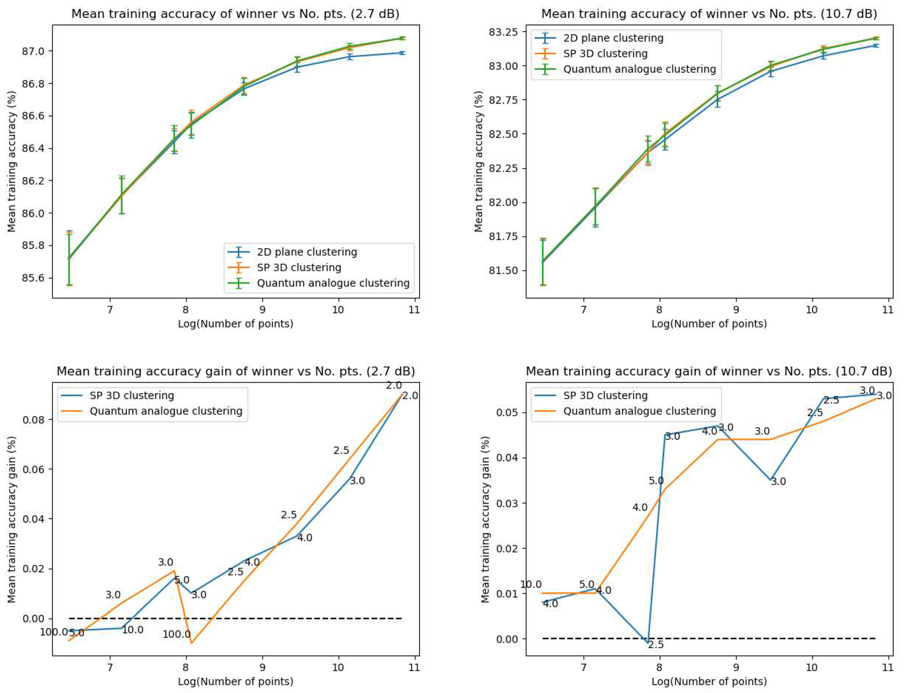
Figure 8 depicts the variation in testing accuracy with the number of points for all three algorithms along with error bars. As mentioned before, this characterises the performance of the algorithms in ‘classification’ mode, that is, when the received points must be decoded in real-time.
Figure 9 portrays the trend in training accuracy with the number of points for all three algorithms along with error bars. This characterises the performance of the algorithms in ‘clustering’ mode, that is, when the received points must be used to update the centroid for future re-classification or if the received datapoints are stored and decoded in batches.
Figure 8 and Figure 9 also plot the gain in testing and training accuracies respectively for the 3DSC-kNN and 2DSC-kNN algorithms. The label of the points in these figures is the radius of ISP for which that accuracy gain was achieved.
Figure 9.
Mean training accuracy (top) and accuracy gain (bottom) v/s the natural log of the number of points for the 2.7 dBm (left) and 10.7 dBm (right) datasets.
Figure 9.
Mean training accuracy (top) and accuracy gain (bottom) v/s the natural log of the number of points for the 2.7 dBm (left) and 10.7 dBm (right) datasets.
- Iteration Performance
In all the figures in this section, the winner is chosen as the radius for which the minimum number of iterations is achieved for the given number of points.
Figure 10 shows how the required number of iterations for all three algorithms varies as the number of points increases. Figure 10 also displays the gain of the 2DSC-kNN and 3DSC-kNN algorithms in the number of iterations to reach their natural endpoints. The label of the points in these figures is the radius of ISP for which that iteration gain was achieved.
- Time Performance
In all the figures in this section, the winner is chosen as the radius for which the minimum execution time is achieved for the given number of points.
Figure 11 puts forth the dependence of testing execution time upon the number of points for all three algorithms along with error bars. As mentioned before, these times are effectively the amount of time the algorithm takes for one iteration. This characterises the performance of the algorithms when performing direct classification decoding of the received points in real time.
This figure reveals the trend in training execution time with the number of points for all three algorithms, along with error bars, as well. This characterises the time performance of the algorithms when performing clustering - that is, when the received points must be used to update the centroid for future re-classification or if the received datapoints are stored and decoded in batches.
Figure 12 graphs the gains in testing and training execution times for the 3DSC-kNN and 2DSC-kNN algorithms.
- Overfitting Performance
Figure 13 exhibits how the overfitting parameter for the 2DEC-kNN k-means clustering, 3DSC-kNN and 2DSC-kNN algorithms vary as the number of points changes.
5.1.2. Discussion and Analysis
From Figure 5 we can see that there is an ideal radius > 1 for which maximum accuracy is achieved. This ideal radius is usually between 2 and 5 for our datasets. For a good choice of radius (>1), the accuracy increases monotonically (with an upper bound) with the number of points, while for a poor choice of radius (<1), the accuracy nosedives as the number of points increases. This is due to the clusters getting squished together near the North pole of the stereographic sphere (the point ). If one is dealing with a large number of points, the accuracy becomes even more sensitive to the choice of radius as the decline in accuracy for a bad radius is much steeper as the number of points increases. These observations hold for both training and testing accuracy (classification and clustering), regardless of the noise in the dataset. All of these observations are also well-reflected in the heatmaps, where one can see that the best training and testing performance is for to 3 and the maximum number of points. It would seem that choosing too large of a radius is not too harmful. This might hold true for the classical algorithms, but in the case when the quantum algorithm is deployed, all the points will be clustered around the South pole of the Bloch sphere and even minimal noise in the quantum circuit will degrade performance. Hence, there is a sweet spot of radius to be chosen.
Figure 7 also shows that there is an ideal radius > 1 for which one needs the minimum number of iterations to reach the natural endpoint. This ideal radius is once again between 2 and 5 for our datasets. As the number of points increases, the number of iterations always increases. For a good choice of radius, the increase is minimal, while for a bad choice, the convergence is very slow. For our experiments, we chose the maximum iterations as 50 hence the observed plateau at 50 iterations. If one is dealing with a large number of points, the convergence becomes more sensitive to the choice of radius. The increase in iterations for a poor choice of radius is much steeper. 2DSC-kNN algorithm and 3DSC-kNN algorithm display near-identical performance.
From Figure 8 we can see that both 2DSC-kNN algorithm and 3DSC-kNN algorithm perform better in accuracy than the 2DEC-kNN algorithm for all datasets. The advantage becomes more definitive as the number of points increases as the increase in accuracy moves beyond the error bar. We observe the highest increase in accuracy for the 2.7 dBm dataset.
In Figure 9 one can see the noticeably better performance of the 2DSC-kNN algorithm and 3DSC-kNN algorithm over the 2DEC-kNN algorithm for all datasets than in the testing case (classification mode). Once again the 2.7 dBm dataset shows the maximum increase. The advantage again becomes more definitive as the number of points increases as the increase in accuracy moves beyond the error bar. The 2DSC-kNN algorithm and 3DSC-kNN algorithm show an almost identical performance.
From Figure 8 and Figure 9 we can also see that almost universally for both algorithms, the gain is greater than 0, i.e. we beat the 2DEC-kNN algorithm in nearly every case! We can also see that the best radius is almost always between 2 and 5. Another observation is that the gain in training accuracy increases with the number of points. The figures further display how similarly the 3DSC-kNN algorithm and 2DSC-kNN algorithm perform in terms of accuracy, regardless of noise.
From Figure 10 it can be concluded that for low noise datasets, since the number of iterations is already quite low, there is not much gain or loss; all 3 algorithms perform almost identically. For high-noise datasets, however, both the 3DSC-kNN algorithm and 2DSC-kNN algorithm show significant improvement in performance, especially for a higher number of points. For a high number of points, the improvement is beyond the error bars and hence very significant. It can be noticed that the ideal radius for minimum iterations is once again between 2 and 5. Here also the 3DSC-kNN algorithm and 2DSC-kNN algorithm perform similarly, with the 2DSC-kNN algorithm performing better in certain cases.
One learns from Figure 11 that most importantly, the 2DSC-kNN algorithm and 2DEC-kNN algorithm take nearly the same amount of time for execution in classification mode, and the 2DSC-kNN algorithm in most cases beats the 3DSC-kNN algorithm. Here too, the gain is significant since it is much beyond the error bar. The execution time increases linearly with the number of points, as expected. These conclusions are supported by Figure 12.
Since the 2DSC-kNN algorithm takes almost the same time, and provides greater accuracy, it is an ideal candidate to replace the 2DEC-kNN algorithm for classification applications.
Figure 11 also shows that all 3 algorithms take almost the same amount of time for training, i.e. in clustering mode. The 3DSC-kNN and 2DSC-kNN algorithms once again perform almost identically, almost always slightly worse than 2DEC-kNN clustering. Figure 12 supports these observations. Here execution time increases linearly with the number of points as well, as one would expect.
In Figure 13, all 3 algorithms have nearly identical performance. As expected. the overfitting decreases with an increase in the number of points.
5.2. Experiment 2: Stopping criterion
Based on the results obtained from the first experiment, we performed another experiment to see how the accuracy of the algorithms varies iteration by iteration. It was observed that the natural endpoint of the algorithm was rarely the ideal endpoint in terms of performance, and hence we wished to observe the performance of each algorithm as the number of iterations progressed.
In this experiment, the entire random subset of datapoints was used for the clustering algorithm. The algorithms were run on the dataset, and the accuracy of the algorithms at each iteration as well as the iteration number of the natural endpoint was recorded. The maximum number of iterations was once again 50. By repeating this 100 times for each number of points (and radius, if applicable), we obtained the general performance variation of each algorithm with the iteration number. The input variables were the number of points, the radius of the stereographic sphere and the iteration number; the recorded performance parameters were the accuracy and probability of stopping.
This experiment revealed that the natural endpoint was indeed a poor choice of stopping criterion, and that endpoint should be chosen as per some “loss function”. It also revealed some important trends in the performance parameters which not only emphasised the importance of the choice of radius and number of points but also gave greater insight into the disadvantages and advantages of each algorithm.
5.2.1. Results
- Characterisation of the 2DSC-kNN algorithm
Figure 14 depicts the dependence of the accuracy of the 2DSC-kNN algorithm upon the iteration number and projection radius for the 2.7 dBm dataset. The figures for the rest of the datasets follow the same trends and are nearly identical in shape.
Figure 15 shows the dependence of the probability of the 2DSC-kNN algorithm reaching its natural endpoint versus the radius of projection and iteration number for the 10.7 dBm dataset with 51200 points and for the 2.7 dBm dataset with 640 points. Once again, the figures for the rest of the datasets follow the same trends and their shape can be extrapolated from the presented Figure 15.
- Comparison with 2DEC-kNN and 3DS-kNN K-Means Clustering
Figure 16 portrays the gain of the 2DSC-kNN and 3DSC-kNN algorithms in the number of iterations to reach maximum accuracy for the 2.7 and 10.7 dBm datasets. In these figures, a gain of ‘g’ means that the algorithm took ‘g’ fewer iterations than the classical k means acting upon the 2D dataset did to reach maximum accuracy.
Figure 17 plots the gain of the 2DSC-kNN and 3DSC-kNN algorithms in the maximum achieved accuracy for the 2.7 and 10.7 dBm datasets. Here, a gain of ‘g’ means that the algorithm was more accurate than the maximum accuracy of the classical k means acting upon the 2D dataset.
Lastly, Figure 18 illustrates the maximum accuracies achieved by the 2DSC-kNN, 3DSC-kNN, and 2DEC-kNN algorithms for the 2.7 and 10.7 dBm datasets.
5.2.2. Discussion and Analysis
Figure 14 shows that once again, there is an ideal radius for which maximum accuracy is achieved. The ideal projection radius is larger than one, in particular, it seems to be between two and five. Most importantly, there is an ideal number of iterations for maximum accuracy, beyond which the accuracy reduces. As the number of points increases, the sensitivity of the accuracy to radius increases significantly. For a bad choice of radius, accuracy only falls with an increase in the number of iterations and stabilises at a very low value. For a good radius, accuracy increases to a point as iterations proceed, and then stabilises at a slightly lower value. If the allowed number of iterations is restricted, the choice of radius to achieve the best results becomes extremely important. With a good radius one can achieve nearly the maximum possible accuracy with very few iterations. As mentioned before, this holds true for all dataset noises. As the dataset noise increases, the iteration number at which maximum accuracy is achieved also expectedly increases. Since accuracy always falls after a point, it is important to choose a stopping criterion rather than wait for the algorithm to reach its natural endpoint. An idea for the stopping criterion is to record the sum of the average dissimilarity for each centroid at each iteration and stop the algorithm if that quantity increases.
Figure 15 portrays that for a good choice of radius, the 2DSC-kNN algorithm approaches convergence much faster. For the algorithm converges much slower or never converges. As the number of points increases, the rate of convergence for poor radius falls dramatically. For a radius greater than the ideal radius as well, the rate of convergence is lower. As one would expect, as dataset noise increases, the algorithm takes longer to converge. As we mentioned before, if the number of iterations is severely limited, the choice of radius becomes very important. If chosen well, the algorithm can reach its ideal endpoint in very few iterations.
Through Figure 16 we see that for lower values of noise, both algorithms do not produce much advantage in terms of iteration gain, regardless of the number of points in the data set. However, at higher noises in the dataset and a high number of points, both algorithms significantly outperform the classical one. This effect is especially significant for the 2DSC-kNN algorithm. For the highest noise and all the points, it saves over 20 iterations compared to the 2DEC-kNN algorithm - an advantage of over 50%. One of the reasons for this is that at low noises, the algorithms already perform quite well, and it is at high noise with a high number of points that the algorithm is stressed enough to reveal the difference in performance. It should be noted that these gains are much higher than when the algorithms are allowed to reach their natural endpoint, suggesting another reason for choosing an ideal stopping criterion.
Figure 17 shows that for all datasets and numbers of points, the 2 algorithms perform better than 2DEC-kNN clustering. The 3DSC-kNN algorithm and 2DSC-kNN algorithms perform nearly the same, and the accuracy gain seems to stabilise with an increase in the number of points. Figure 18 supports these conclusions.
5.3. Overall Observations
- Overall observations from Experiment 1
- 1.
- The ideal radius of projection is greater than 1 and between 2 and 5. At this ideal radius, one achieves maximum testing and training accuracy, and minimum iterations.
- 2.
- In general, the accuracy performance is the same for 3DSC-kNN and 2DSC-kNN algorithms - this shows a significant contribution of the ISP to the advantage as opposed to ‘quantumness’. This is a very significant distinction, not made by any other previous work. The 2DSC-kNN algorithm generally requires fewer iterations to achieve the ideal accuracy, however.
- 3.
- 2DSC-kNN and 3DSC-kNN algorithms lead to an increase in the accuracy performance in general, with the increase most pronounced for the 2.7 dBm dataset.
- 4.
- The 2DSC-kNN algorithm and 3DSC-kNN algorithm give more iteration performance gain (fewer iterations required than 2DEC-kNN) for high noise datasets and for a large number of points.
- 5.
- Generally, increasing the number of points works in favour of the 2DSC-kNN and 3DSC-kNN algorithms, with the caveat that a good radius must be carefully chosen.
- Overall observations from Experiment 2
- 1.
- These results further stress the importance of choosing a good radius (2 to 5 in this application) and a better stopping criterion. The natural endpoint is not suitable.
- 2.
- The results clearly justify the fact that the developed 2DSC-kNN algorithm has significant advantages over 2DEC-kNN k-means clustering and 3DSC-kNN clustering.
- 3.
- The 2DSC-kNN algorithm performs nearly the same as the 3DSC-kNN algorithm in terms of accuracy, but for iterations to achieve this max accuracy, the 2DSC-kNN algorithm is better (especially for high noise and a high number of points).
- 4.
- The developed 2DSC-kNN algorithm and 3DSC-kNN algorithm are better than the 2DEC-kNN algorithm in general - in terms of both accuracy and iterations to reach that maximum accuracy.
6. Conclusion and Further work
This work considers the practical case of performing k-nearest neighbour clustering on experimentally acquired 64-QAM data. This work has described the problem in detail and explained how the Stereographic Quantum K Nearest-Neighbour Clustering and its classical analogue, the 2DSC-kNN algorithm, can be used. The proposed processes and circuits as well as the theoretical justification for the Stereographic Quantum K Nearest-Neighbour Clustering quantum algorithm and the 2DSC-kNN classical algorithm have been described in detail. Finally, the simulation results on the real-world datasets have been presented, along with relevant analysis. From the analysis, one can clearly see that the Stereographic Quantum K Nearest-Neighbour Clustering and especially its classical analogue is something that should be considered for industrial implementation - the experiments provide a proof of concept. It also shows the importance of choosing the projection radius. In addition, from Appendix E one can see by the distance estimate (Equation (A34)) for SQ-kNN clustering that it is expected to perform better than quantum k-means clustering with standard angle embedding. These results clearly warrant the practical implementation and testing of both quantum and classical algorithms.
Quantum and quantum-inspired computing has the potential to change the way certain algorithms are performed, with potentially significant advantages. However, as the field is still in relative infancy, finding where quantum and quantum-inspired computing fits in practice is a challenging problem. Here, we have seen that quantum and quantum-inspired computing can indeed be applied to signal-processing scenarios, and could potentially work well in the noisy quantum era as clustering algorithms that are relatively robust to noise and inaccuracy.
6.1. Future work
One of the most important directions of future work is to experiment with more diverse datasets. More experimentation may also lead to more sophisticated methods of selecting the radius for ISP. A more detailed analysis of how to choose a radius of projection through analytical methods is another important direction for future work. A differential geometric analysis of the effects of the ISP on a square grid gives a rough intuition of why one needs an appropriate radius. A comparison with amplitude embedding is also warranted. The ellipsoidal projection (Appendix D) is another promising and novel idea that is to be explored further. In this project, two different stopping criteria for the algorithm were proposed and revealed a change in its performance; yet there is plenty of room to explore more possible stopping criteria.
Further directions of study include improved overlap estimation methods [48] and communication scenarios where the dimensionality of the data points is greatly increased. For example, when multiple carriers experience identical or at least systematically correlated phase rotations.
Another future work is to benchmark against sampling-based quantum-inspired algorithms. As part of a research analysis to evaluate the best possibilities for achieving a practical speed-up, we investigated the landscape of classical algorithms inspired by the sampling in quantum algorithms. Initially, we found that such algorithms have theoretical complexity competing with quantum algorithms, however only under arguably unrealistic assumptions on the structure of the classical data. As the performance of the quantum algorithms turns out to be extremely poor, this reopens the possibility that quantum-inspired algorithms can actually yield performance improvements while we wait for quantum computers with sufficiently low noise. Thus future work will also be a practical implementation of the quantum-inspired k nearest-neighbour clustering algorithm [12], with the goal of testing the computational advantage over 2DEC-kNN, 3DSC-kNN, and 2DSC-kNN algorithms.
Funding
This work was funded by the TUM-Huawei Joint Lab on Algorithms for Short Transmission Reach Optics (ASTRO). This project has received funding from the DFG Emmy-Noether program under grant number NO 1129/2-1 (JN) and by the Federal Ministry of Education and Research of Germany in the programme of ”Souveran. Digital. Vernetzt.”. Joint project 6G-life, project identification number: 16KISK002, and of the Munich Center for Quantum Science and Technology (MCQST).
Data Availability Statement
All source codes and the complete set of generated graphs are available through the publicly accessible GitHub repository at the following link: https://github.com/AlonsoViladomat/Stereographic-quantum-embedding-clustering. The datasets are not published and are a property of Huawei Technologies.
Acknowledgments
We would like to acknowledge fruitful discussions with Stephen DiAdamo and Fahreddin Akalin during the initial stages of the project.
Conflicts of Interest
The authors declare no conflict of interest.
Abbreviations
A list of abbreviations used in this manuscript can be found in below.
| ADC | Analog-to-digital converter |
| CD | Chromatic dispersion |
| CFO | Carrier frequency offset |
| CPE | Carrier phase estimation |
| DAC | Digital-to-analog converter |
| DP | Dual Polarisation |
| ECL | External cavity laser |
| FEC | Forward error correction |
| GHz | Gigahertz |
| GBd | Gigabauds |
| GSa/s | samples per second |
| DSP | Digital signal processing |
| ISP | Inverse stereographic projection |
| MIMO | Multiple input multiple output |
| M-QAM | M-ary Quadrature Amplitude Modulation |
| QML | Quantum Machine Learning |
| QRAM | Quantum Random Access Memory |
| TR | Timing recovery |
| SQ access | Sample and query access |
| kNN | K Nearest Neighbour (Definition 3) |
| FF-QRAM | Flip flop QRAM |
| NISQ | Near-intermediate scale quantum |
| Dataspace | |
| D | Dataset |
| D | 2-dimensional dataset |
| set of all M centroids | |
| Cluster associated to a centroid | |
| Dissimilarity (measure function) | |
| Euclidean dissimilarity | |
| Cosine dissimilarity | |
| ISP into a sphere of radius r | |
| n-sphere of radius r | |
| Hilbert space of one qubit | |
| nDEC-kNN | n-dimensional Euclidean Classical k Nearest-Neighbour algorithm (Definition 4) |
| SQ-kNN | Stereographic Quantum k Nearest-Neighbour algorithm (Definition 10) |
| 2DSC-kNN | 2D Stereographic Classical k Nearest-Neighbour algorithm (Definition 12) |
| 3DSC-kNN | 3D Stereographic Classical k Nearest-Neighbour algorithm (Definition 6) |
Appendix A. QAM and Data Visualisation
Quadrature amplitude modulation (QAM) conveys multiple digital bits with each transmission by mixing both amplitude and phase variations in a carrier frequency, by changing (modulating) the amplitudes of two carrier waves. The two carrier waves (of the same frequency) are out of phase with each other by 90; namely, they are the sine and cosine waves of a given frequency. This condition is known as orthogonality and the two carrier waves as quadrature. The transmitted signal is created by adding the two carrier waves (the sine and cosine components) together. At the receiver, the two waves can be coherently separated (demodulated) because of their orthogonality. QAM is used extensively as a modulation scheme for digital telecommunication systems, such as in 802.11 Wi-Fi standards. Arbitrarily high spectral efficiencies can be achieved with QAM by setting a suitable constellation size, limited only by the noise level and linearity of the communications channel [50]. QAM allows us to transmit multiple bits for each time interval of the carrier symbol. The term “symbol” means some unique combination of phase and amplitude [51].
In this work, each transmitted signal corresponds to a complex number :
where is the initial transmission power and is the phase of s. The case shown in Equation (A1) is ideal; however, in real-world systems, noise affects the transmitted signal, distorting it and scattering it in the amplitude and phase space. For our case, the received and partially processed noisy signal can be modelled as:
where is a random noise affecting the overall value of ideal amplitude and phase. This model motivates the use of nearest neighbour clustering for cases when the noise causes the received signal to be scattered in the vicinity of the ideal signal s.
Appendix A.1. Description of 64-QAM Data
In this section, the various datasets collected by us through the setup described in Section 2.1 are visualised. As mentioned, there are 4 datasets with launch powers of dBm, corresponding to various noise levels. Each data set consists of 3 variables:
- ‘alphabet’: The initial analog values at which the data was transmitted, in the form of complex numbers i.e. for an entry (), the transmitted signal was of the form . Since the transmission protocol is 64-QAM, there are 64 values in this variable. The transmission alphabet is the same irrespective of the nonlinear distortions.
- ‘rxsignal’: The received analog values of the signal by the receiver. This data is in the form of a matrix. Each datapoint was transmitted 5 times to the receiver, and so each row contains the values detected by the receiver during the different instances of the transmission of the same datapoint. The values in different rows represent unique datapoint values detected by the receiver.
- ‘bits’: This is the true label for the transmitted points. This data is in the form of a matrix. Since the protocol is 64-QAM, each analog point represents 6 bits. These 6 bits are the entries in each column, and each value in a different row represents the correct label for a unique transmitted datapoint value. The first 3 bits encode the column and the last 3 bits encode the row - see Figure A3.
In Figure A1, we can see the analog transmission values (alphabet) for all the different channels. In the next 4 figures (Figure A2a to Figure A2d) we can observe the transmission data for all the iterations for each channel. The first transmission data is represented as blue crosses, the second transmission as orange circles, the third transmission as yellow dots, the fourth transmission as purple stars, and the fifth transmission as green pluses. The de-mapping alphabet is depicted in Figure A3.
Figure A1.
The analog alphabet (initial analog transmission values) for the data transmitted in all the channels. The real part represents the amplitude of the transmitted sine wave and the imaginary part represents the amplitude of the cosine wave.
Figure A1.
The analog alphabet (initial analog transmission values) for the data transmitted in all the channels. The real part represents the amplitude of the transmitted sine wave and the imaginary part represents the amplitude of the cosine wave.
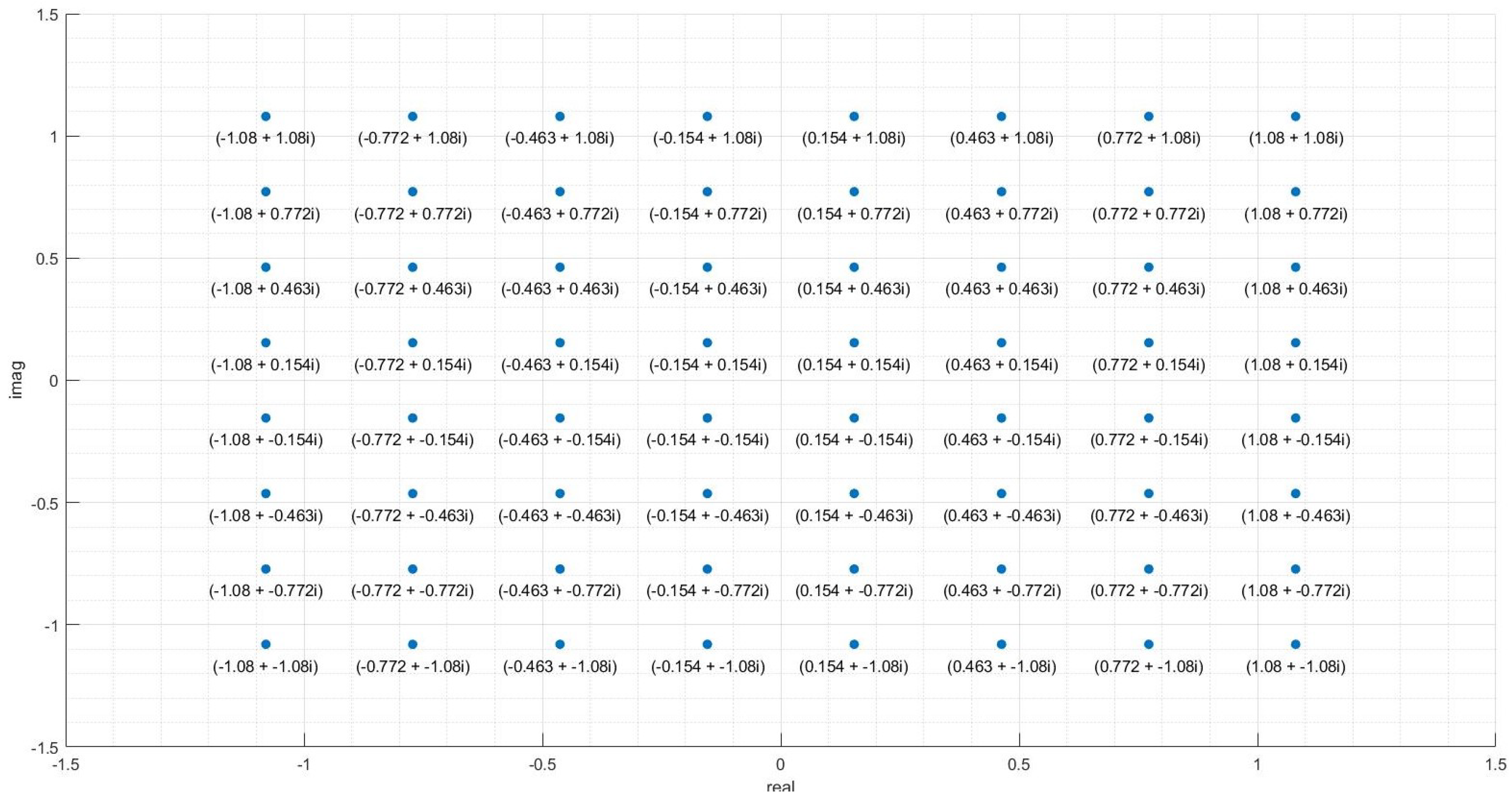
Figure A2.
The 4 datasets detected by the receiver with various launch powers corresponding to different noise levels. All 5 iterations of transmission are depicted together.
Figure A2.
The 4 datasets detected by the receiver with various launch powers corresponding to different noise levels. All 5 iterations of transmission are depicted together.
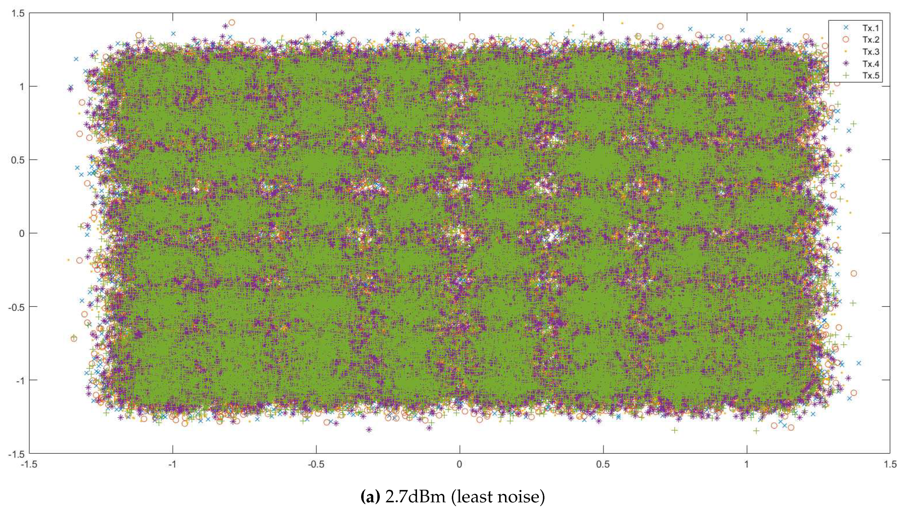
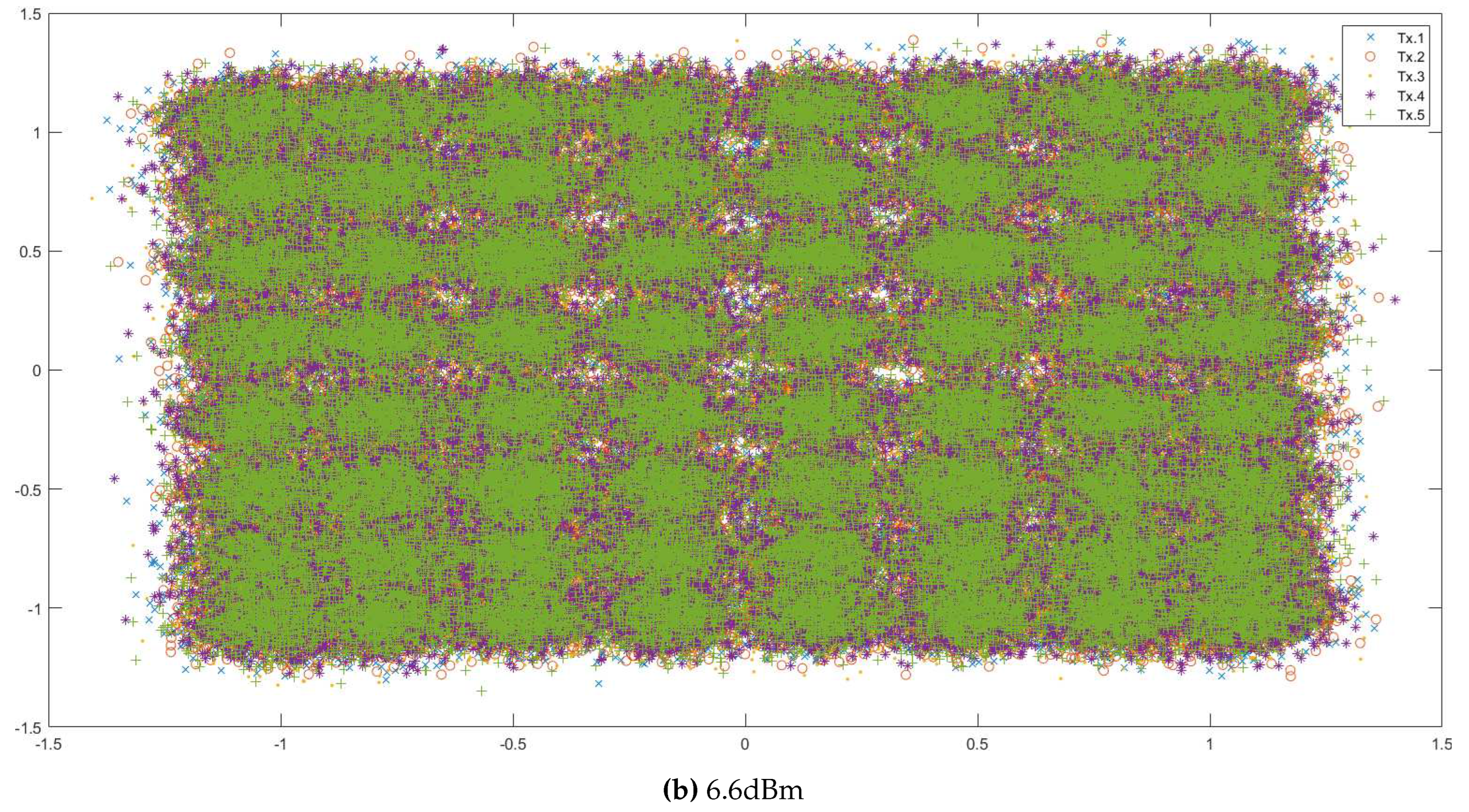
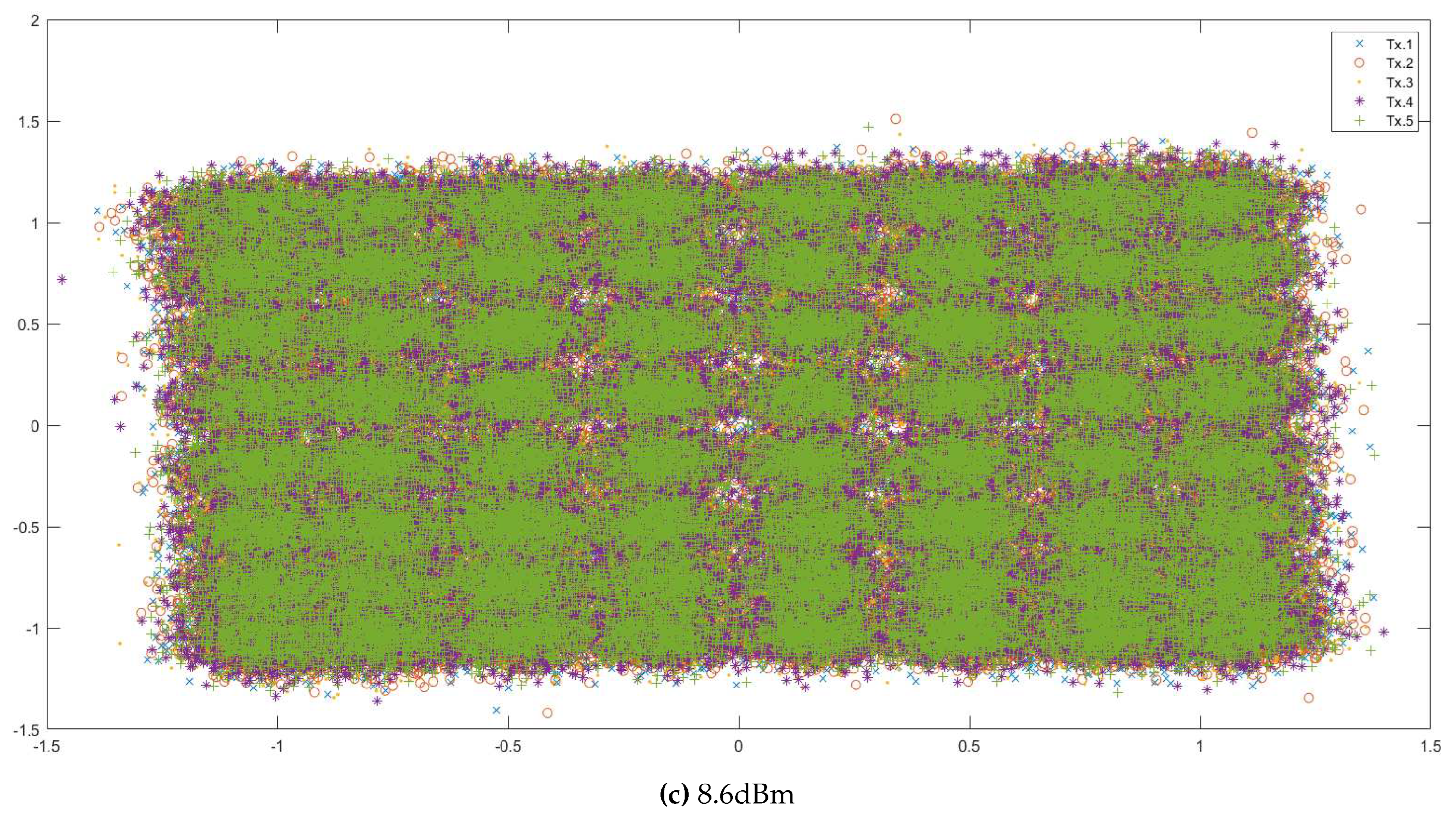
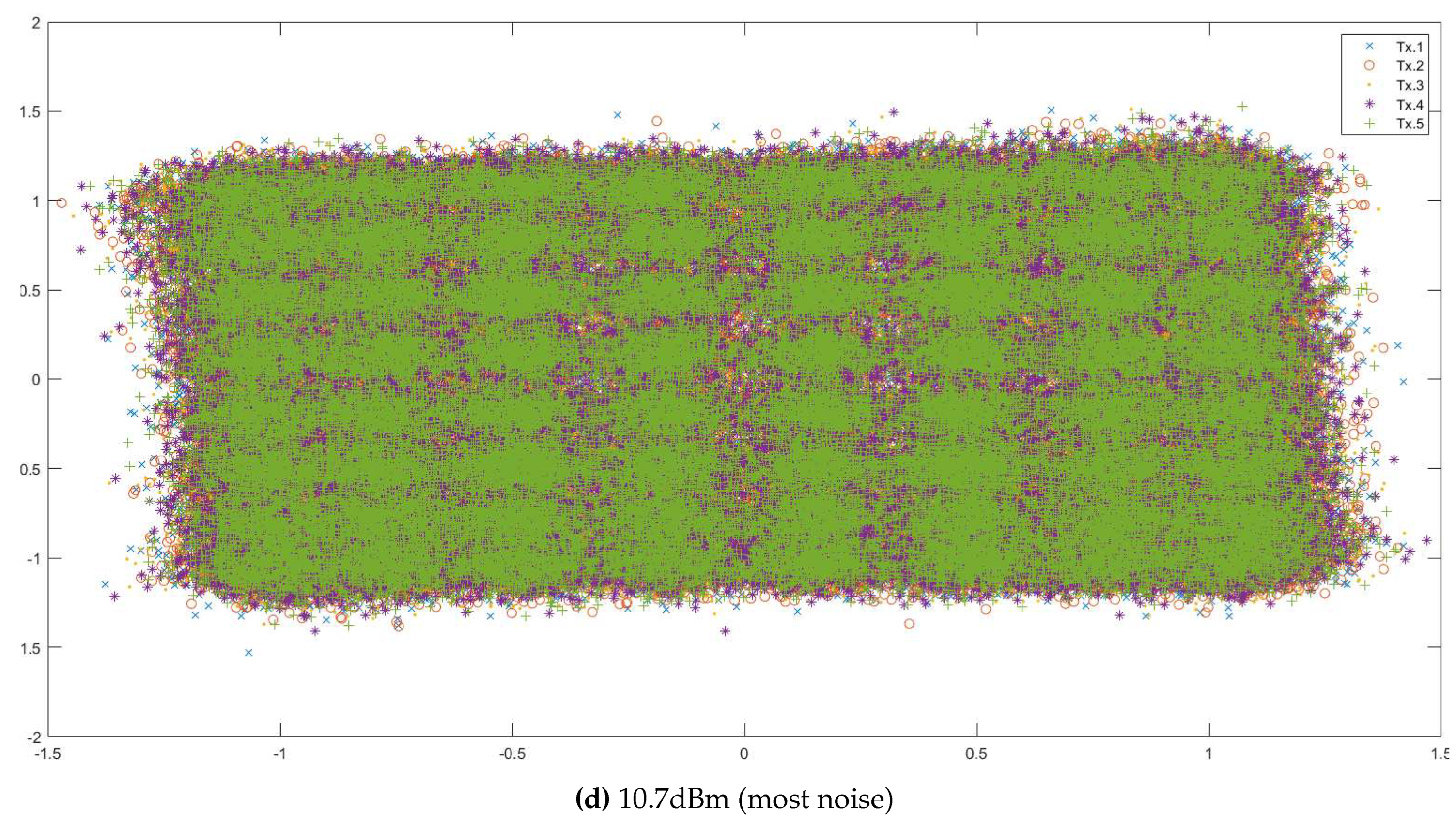
Figure A3.
The bitstring mapping and demapping alphabet.
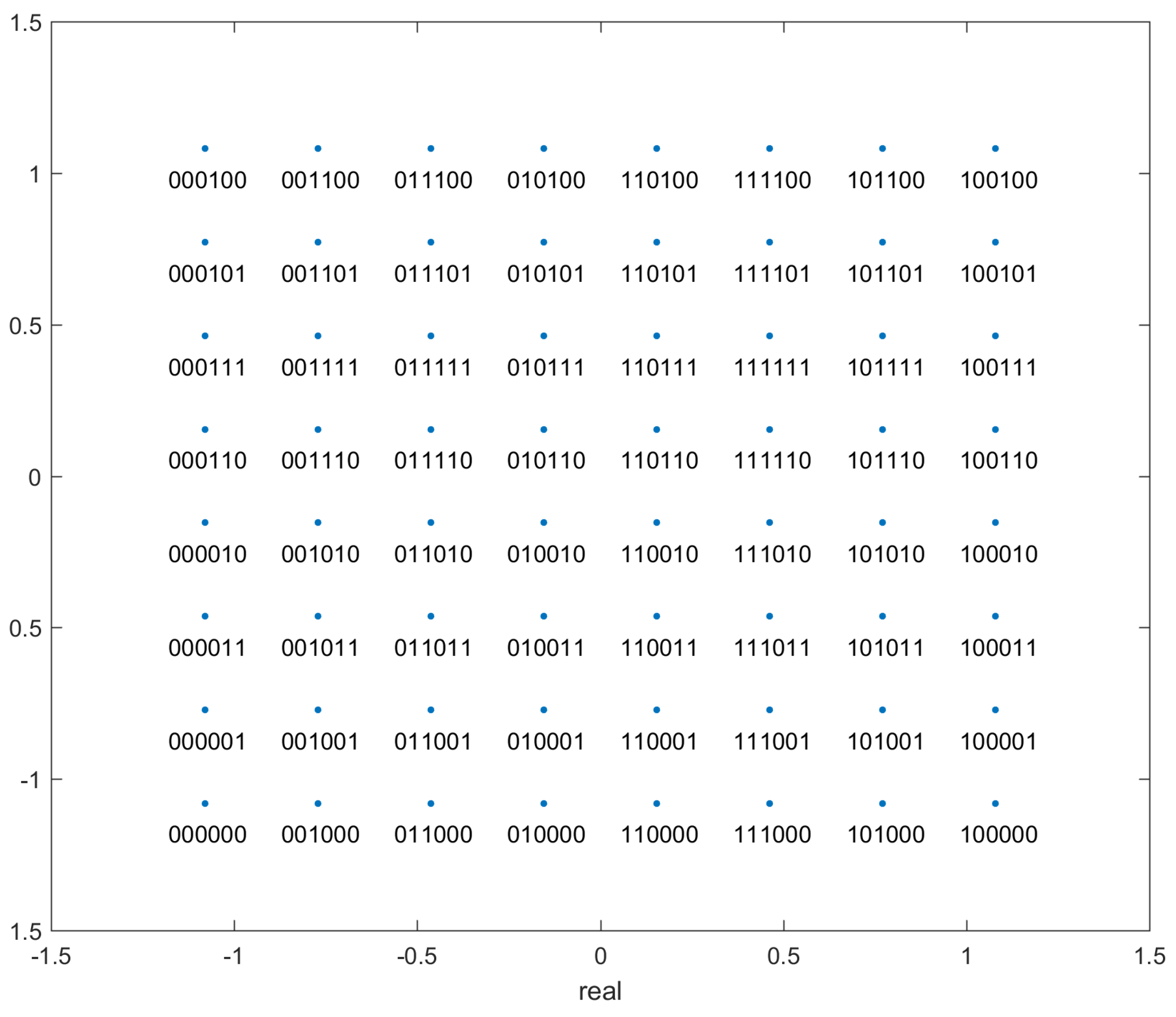
One can see from these figures that as the noise in the channel increases, the points are further scattered away from the initial alphabet. In addition, the non-linear noise effects also increase, causing distortion of the ‘shape’ of the data, most clearly visible in Figure A2d - especially near the ‘corners’. The birefringence phase noise also increases with an increase in the channel noise causing all the points to be ‘rotated’ about the origin.
Once the centroids have been found and the data has been clustered, as mentioned before, we need to ‘de-map’ the analog centroid values and clusters to bit-strings. For this, we need a de-mapping alphabet which maps the analog values of the alphabet to the corresponding bit strings. The de-mapping alphabet is depicted in Figure A3. It can be seen from the figure that, as in most cases, the points are Gray coded i.e. adjacent points differ in binary translation by only 1 bit. This helps minimise the number of bit errors per symbol error in case of misclassification or exceptionally high noise. In case a point is misclassified, with most probability, it will be assigned to a neighbouring cluster. Since the surrounding clusters differ by only 1 bit, it minimises the bit error rate. Due to Gray coding, the bit error rate is approximately of the symbol error rate.
Appendix B. Data Embedding
One needs data in the form of quantum states for processing in a Quantum Computer. However, due to the instability of current qubits, data can currently only be stored for an extended period of time in classical form. Hence, the need arises to convert classical data into a quantum form. NISQ devices have a very limited number of logical qubits, and these qubits are stable for a very limited period of time. The first step in Quantum Machine Learning is to load classical data by encoding it into qubits. This process is called data encoding or embedding. Classical data encoding for quantum computation plays a critical role in the overall design and performance of quantum machine learning algorithms. Table A1 summarizes the various forms of data embedding.

| Embedding | Encoding | Num. qubits required | Gate Depth |
|---|---|---|---|
| Basis | per data point | ||
| Angle | |||
| Amplitude | gates | ||
| QRAM | queries |
Appendix B.1. Angle Embedding
Angle encoding [47,53,54] is one of the most fundamental forms of encoding classical data into a quantum state. Each data point is represented as a separate qubit. The classical real number is encoded into the rotation angle of the qubit. This encoding, in its most basic form, requires N qubits to represent N dimensional data. It is quite cheap to prepare in terms of complexity – all that is needed is one rotation quantum gate for each qubit. This is one of the forms of encoding we have used in our implementation of quantum kNN clustering. It is generally useful for quantum neural networks and other such QML algorithms. Angle encoding encodes N features into the rotation angles of n qubits where .
The rotations can be chosen as either , or gates. As a first step, each data point of the input is normalized to the interval . To encode the data points, a rotation around the y-axis is used, for which the angle depends on the value of the normalized data point. This creates the following separable state:
It can easily be seen that one qubit is needed per data point, which is not optimal. To load the data, the rotations on the qubits can be performed in parallel; thus, the depth of the circuit is optimal [47].
The main advantage of this encoding is that it is very efficient in terms of operations – only a constant number of parallel operations are needed regardless of how many data values need to be encoded. This is not optimal from a qubit point of view (the circuit is very wide), as every input vector component requires one qubit. Another related encoding, called dense angle encoding, exploits an additional property of qubits (relative phase) to use only qubits to encode n data points. QRAM can be used to generate the more compact quantum state
Appendix C. Stereographic Projection
Appendix C.1. ISP for General Radius
In this appendix, the transformations for obtaining the cartesian co-ordinates of the projected point on a sphere of general radius are derived, followed by the derivation of polar and azimuthal angles of point on the sphere. First mentioned are 3 conditions that the point on the sphere must satisfy, and then follows the rest of the derivation. Refer to Figure A4 for better understanding of the conditions and calculations.
Figure A4.
ISP for a sphere of radius ‘r’. In this figure, the plane is the plane of angle with respect to the X-axis perpendicular to the XY plane, i.e. the plane containing the 2D point and it projection.
Figure A4.
ISP for a sphere of radius ‘r’. In this figure, the plane is the plane of angle with respect to the X-axis perpendicular to the XY plane, i.e. the plane containing the 2D point and it projection.
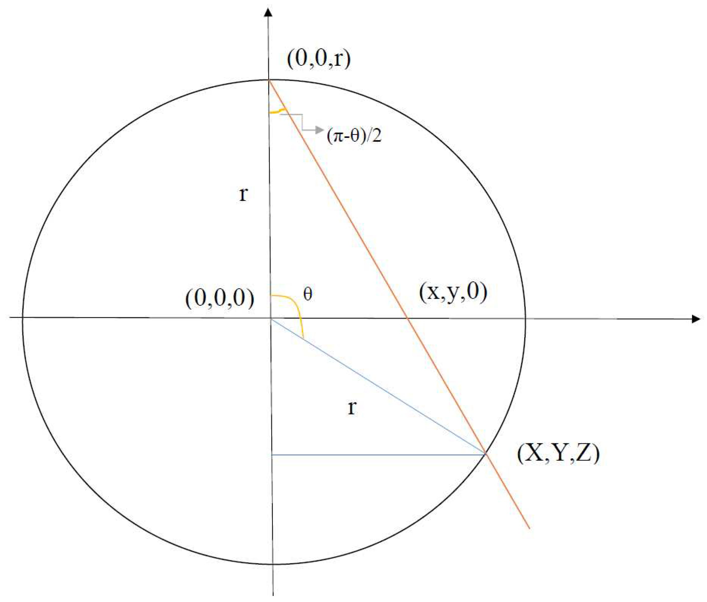
- 1.
- Azimuthal angle of the original point and the projected point must be the same, i.e. the original point, projected point, and the top of the sphere (the point from which all projections are drawn) lie on the same plane, which is perpendicular to the 2D plane.
- 2.
- The projected point lies on the sphere.
- 3.
- The triangle with vertices , and is similar to the triangle with vertices , and :
Using Equation (A7) and Equation (A5), we get
Substituting in Equation (A6) we get,
Hence one gets the set of transformations:
Calculating the polar angle () and azimuthal angle ():
Appendix C.2. Equivalence of displacement and scaling
Refer to Figure A5. Here, is the point from which all the projections originate; and are the centres of the projection spheres of radius and respectively; is the point on the 2D plane to be projected; and and are the ISP of P on the spheres of radius and centre and radius and centre respectively.
Figure A5.
ISP on a sphere displaced above the plane and a sphere centred at origin.
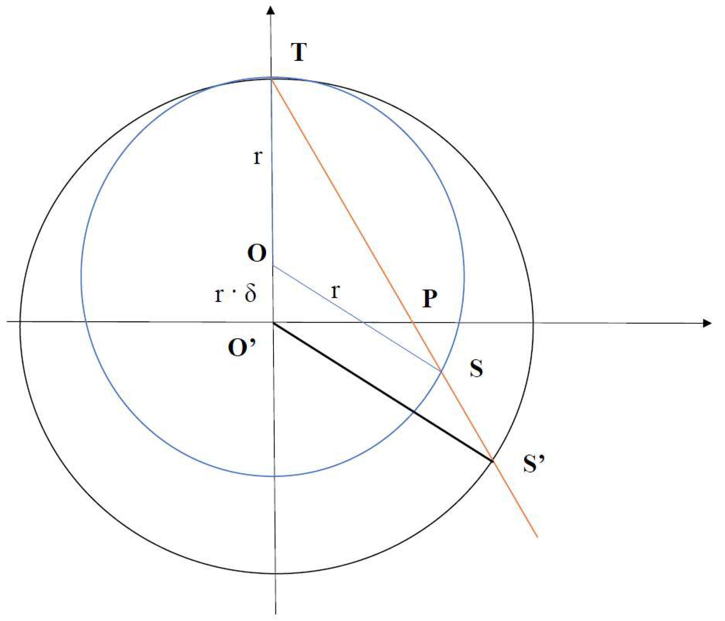
Also,
Hence
Since both and lie on the same plane, which is a vertical cross section of the sphere (plane perpendicular to the data plane and passing through the centre of both stereographic spheres), the azimuthal angle of both points is equal ().
Hence one can see that the azimuthal and the polar angle generated by ISP on a sphere of radius displaced above the 2D plane containing the points by is the same as the azimuthal and the polar angle generated by ISP on a sphere of radius centred at origin. This reduces the effective number of parameters that can be chosen for the embedding.
Appendix D. Ellipsoidal Embedding
Here, we first derive the transformations for obtaining the cartesian co-ordinates of the projected point on a general ellipsoid, followed by the derivation of polar and azimuthal angles for the point on the ellipsoid. First mentioned are three conditions that the point on the sphere must satisfy, and then follows the rest of the derivation. Refer to Figure A6 for a better understanding of the conditions and calculations.
Figure A6.
Ellipsoidal Projection: a generalisation of the ISP.
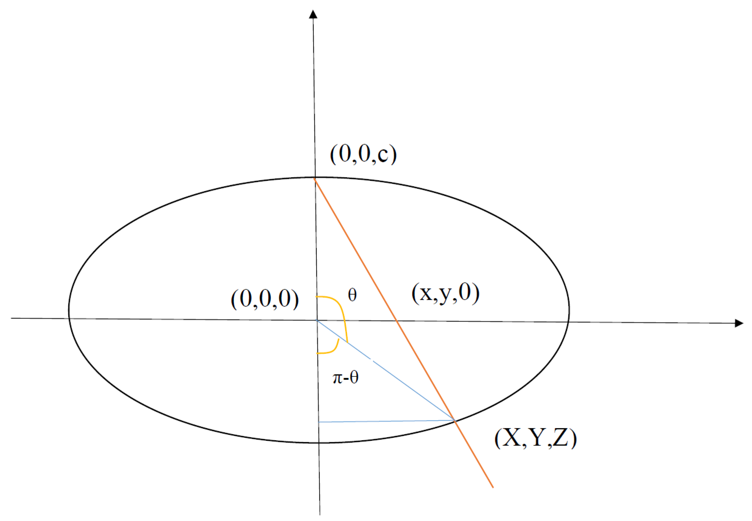
- 1.
- Azimuthal angle -
- 2.
- The projected point lies on the ellipsoid -
- 3.
- The triangle with vertices , and is similar to the triangle with vertices , and -
From the above conditions, we have
Substituting as before, we get
Hence one gets the set of transformations:
From Figure A6 one can see that
Now that we have these expressions, we have 2 methods of encoding the datapoint. We can either encode it as before, using the unitary which would correspond to projecting all the points on the ellipsoid to the surface of the sphere radially; or, we could use mixed states to represent the points on the surface of the ellipsoid after rescaling it to lie within the Bloch sphere.
Appendix E. Distance Estimation using Stereographic Embedding
In our proposed quantum algorithm (the SQ-kNN algorithm), we project the original 2-dimensional points into the stereographic sphere, before converting them into quantum states using angle embedding and then estimating the overlap with the Bell state measurement circuit. Due to the many steps of this procedure, it is insightful to calculate the final output in terms of the original input, the 2-dimensional datapoints. It also serves as a useful point of comparison with the 2DEC-kNN algorithm, where the Euclidean dissimilarity between the 2-dimensional points is used for classification.
Recall Equation (50) from Section 2.7. Then concatenating the ISP with the cosine dissimilarity, we get a new dissimilarity as follows.
As mentioned before, we begin with two 2D points , and compute
To calculate this, we compute using Equation (50):
Combining, we have:
where is the Euclidean dissimilarity from Equation (25).
It is illustrative to pick the point (origin) and see how this function varies as the other point varies. In this case, we have:
For Figure A7, the radius of the stereographic sphere is assumed to be one. Hence the quantum dissimilarity reduces to:
For Figures A8 and A9, the radius of the stereographic sphere is assumed to be 2 and respectively.
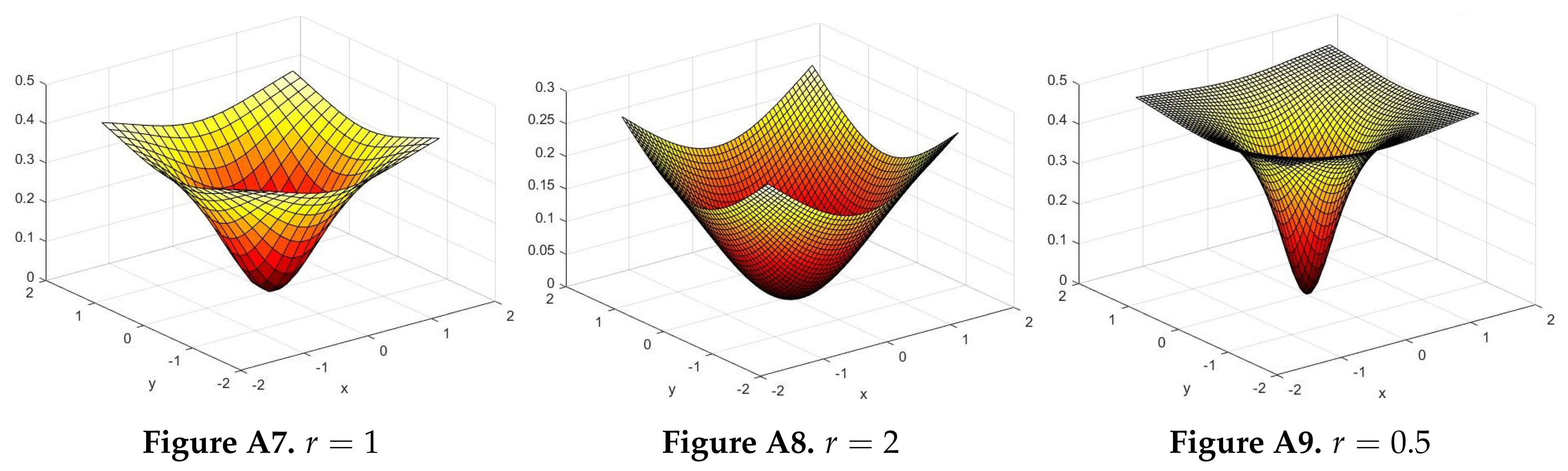 |
Appendix F. Rotation Gates and the UGate
The complete expression for the unitary UGate in Qiskit is as follows:
Using the state for encoding, we have
One can see that there is no dependence of this state on . On the other hand, if we use the state for encoding, we have
One can see that the term leads only to a global phase. A global phase will not affect the observable outcome of the SWAP test or Bell-state measurement (due to the modulus operator) - hence once again, no information can be encoded into the quantum state using .
For constructing the point () on the Bloch sphere, we can use rotation gates as well:
From Equation (A41) one can see that and only differ by a global phase (). Hence, the and operations can be used interchangeably for state preparation since a global phase will not affect the observable result of the SWAP test.
References
- Harrow, A.W.; Hassidim, A.; Lloyd, S. Quantum Algorithm for Linear Systems of Equations. Physical Review Letters 2009, 103. [Google Scholar] [CrossRef] [PubMed]
- Lloyd, S.; Mohseni, M.; Rebentrost, P. Quantum algorithms for supervised and unsupervised machine learning. arXiv 2013, arXiv:1307.0411 2013. [Google Scholar]
- Preskill, J. Quantum Computing in the NISQ era and beyond. Quantum 2018, 2, 79. [Google Scholar] [CrossRef]
- Tang, E. Quantum Principal Component Analysis Only Achieves an Exponential Speedup Because of Its State Preparation Assumptions. Physical Review Letters 2021, 127. [Google Scholar] [CrossRef]
- Arute, F.; Arya, K.; Babbush, R.; Bacon, D.; Bardin, J.; Barends, R.; Biswas, R.; Boixo, S.; Brandao, F.; Buell, D.; Burkett, B.; et al. Quantum Supremacy using a Programmable Superconducting Processor. Nature 2019, 574, 505–510. [Google Scholar] [CrossRef] [PubMed]
- Schuld, M.; Petruccione, F. Supervised Learning with Quantum Computers; Quantum Science and Technology; Springer International Publishing, 2018. [Google Scholar]
- Schuld, M.; Sinayskiy, I.; Petruccione, F. An introduction to quantum machine learning. arXiv 2014, arXiv:1409.3097. [Google Scholar] [CrossRef]
- Kerenidis, I.; Prakash, A. Quantum Recommendation Systems. In Proceedings of the 8th Innovations in Theoretical Computer Science Conference (ITCS 2017); Leibniz International Proceedings in Informatics (LIPIcs). Papadimitriou, C.H., Ed.; Schloss Dagstuhl–Leibniz-Zentrum fuer Informatik: Dagstuhl, Germany, 2017; Volume 67, pp. 49:1–49:21. [Google Scholar] [CrossRef]
- Kerenidis, I.; Landman, J.; Luongo, A.; Prakash, A. q-means: A quantum algorithm for unsupervised machine learning. arXiv 2018, arXiv:1812.03584 2018. [Google Scholar]
- Pakala, L.; Schmauss, B. Non-linear mitigation using carrier phase estimation and k-means clustering. Photonic Networks; 16. ITG Symposium. VDE. 2015; 1–5. [Google Scholar]
- Zhang, J.; Chen, W.; Gao, M.; Shen, G. K-means-clustering-based fiber nonlinearity equalization techniques for 64-QAM coherent optical communication system. Optics express 2017, 25, 27570–27580. [Google Scholar] [CrossRef]
- Tang, E. Quantum Principal Component Analysis Only Achieves an Exponential Speedup Because of Its State Preparation Assumptions. Phys. Rev. Lett. 2021, 127, 060503. [Google Scholar] [CrossRef]
- Gambetta, J. IBM’s roadmap for scaling quantum technology.
- Martyn, J.M.; Rossi, Z.M.; Tan, A.K.; Chuang, I.L. A grand unification of quantum algorithms. arXiv 2021, arXiv:2105.02859 2021. [Google Scholar] [CrossRef]
- Kopczyk, D. Quantum machine learning for data scientists. arXiv 2018, arXiv:1804.10068 2018. [Google Scholar]
- Esma Aimeur, G.B.; Gambs, S. Quantum clustering algorithms. ICML ’07: Proceedings of the 24th international conference on Machine learning June 2007. 2007; 1–8. [Google Scholar]
- Cruise, J.R.; Gillespie, N.I.; Reid, B. Practical Quantum Computing: The value of local computation. arXiv 2020, arXiv:2009.08513 2020. [Google Scholar]
- Johri, S.; Debnath, S.; Mocherla, A.; Singh, A.; Prakash, A.; Kim, J.; Kerenidis, I. Nearest centroid classification on a trapped ion quantum computer. npj Quantum Information 2021, 7, 122. [Google Scholar] [CrossRef]
- Khan, S.U.; Awan, A.J.; Vall-Llosera, G. K-Means Clustering on Noisy Intermediate Scale Quantum Computers. arXiv 2019, arXiv:1909.12183 2019. [Google Scholar]
- Cortese, J.A.; Braje, T.M. Loading classical data into a quantum computer. arXiv 2018, arXiv:1803.01958 2018. [Google Scholar]
- Giovannetti, V.; Lloyd, S.; Maccone, L. Quantum Random Access Memory. Physical Review Letters 2008, 100. [Google Scholar] [CrossRef]
- Buhrman, H.; Cleve, R.; Watrous, J.; De Wolf, R. Quantum fingerprinting. arXiv 2001. [Google Scholar] [CrossRef]
- Ripper, P.; Amaral, G.; Temporão, G. Swap Test-based characterization of decoherence in universal quantum computers. Quantum Information Processing 2023, 22, 1–14. [Google Scholar] [CrossRef]
- Foulds, S.; Kendon, V.; Spiller, T. The controlled SWAP test for determining quantum entanglement. Quantum Science and Technology 2021, 6, 035002. [Google Scholar] [CrossRef]
- Tang, E. A Quantum-Inspired Classical Algorithm for Recommendation Systems. In Proceedings of the 51st Annual ACM SIGACT Symposium on Theory of Computing; STOC 2019. Association for Computing Machinery: New York, NY, USA, 2019; pp. 217–228. [Google Scholar] [CrossRef]
- Chia, N.H.; Lin, H.H.; Wang, C. Quantum-inspired sublinear classical algorithms for solving low-rank linear systems. arXiv 2018, arXiv:1811.04852 2018. [Google Scholar]
- Gilyén, A.; Lloyd, S.; Tang, E. Quantum-inspired low-rank stochastic regression with logarithmic dependence on the dimension. arXiv 2018, arXiv:1811.04909 2018. [Google Scholar]
- Arrazola, J.M.; Delgado, A.; Bardhan, B.R.; Lloyd, S. Quantum-inspired algorithms in practice. Quantum 2020, 4, 307. [Google Scholar] [CrossRef]
- Chia, N.H.; Gilyén, A.; Li, T.; Lin, H.H.; Tang, E.; Wang, C. Sampling-based sublinear low-rank matrix arithmetic framework for dequantizing Quantum machine learning. In Proceedings of the 52nd Annual ACM SIGACT Symposium on Theory of Computing; 2020. [Google Scholar] [CrossRef]
- Arrazola, J.M.; Delgado, A.; Bardhan, B.R.; Lloyd, S. Quantum-inspired algorithms in practice. Quantum 2020, 4, 307. [Google Scholar] [CrossRef]
- Chia, N.H.; Gilyén, A.; Lin, H.H.; Lloyd, S.; Tang, E.; Wang, C. Quantum-Inspired Algorithms for Solving Low-Rank Linear Equation Systems with Logarithmic Dependence on the Dimension. In Proceedings of the 31st International Symposium on Algorithms and Computation (ISAAC 2020); Leibniz International Proceedings in Informatics (LIPIcs). Cao, Y., Cheng, S.W., Li, M., Eds.; Schloss Dagstuhl–Leibniz-Zentrum für Informatik: Dagstuhl, Germany, 2020; Volume 181, pp. 47:1–47:17. [Google Scholar] [CrossRef]
- Sergioli, G.; Santucci, E.; Didaci, L.; Miszczak, J.A.; Giuntini, R. A quantum-inspired version of the nearest mean classifier. Soft Computing 2018, 22, 691–705. [Google Scholar] [CrossRef]
- Sergioli, G.; Bosyk, G.M.; Santucci, E.; Giuntini, R. A quantum-inspired version of the classification problem. International Journal of Theoretical Physics 2017, 56, 3880–3888. [Google Scholar] [CrossRef]
- Subhi, G.M.; Messikh, A. Simple quantum circuit for pattern recognition based on nearest mean classifier. International Journal on Perceptive and Cognitive Computing 2016, 2. [Google Scholar] [CrossRef]
- Nguemto, S.; Leyton-Ortega, V. Re-QGAN: an optimized adversarial quantum circuit learning framework. arXiv 2022. [Google Scholar] [CrossRef]
- Eybpoosh, K.; Rezghi, M.; Heydari, A. Applying inverse stereographic projection to manifold learning and clustering. Applied Intelligence 2022, 52, 4443–4457. [Google Scholar] [CrossRef]
- Poggiali, A.; Berti, A.; Bernasconi, A.; Del Corso, G.; Guidotti, R. Quantum Clustering with k-Means: a Hybrid Approach. arXiv 2022, arXiv:2212.06691 2022. [Google Scholar]
- de Veras, T.M.L.; de Araujo, I.C.S.; Park, D.K.; da Silva, A.J. Circuit-Based Quantum Random Access Memory for Classical Data With Continuous Amplitudes. IEEE Transactions on Computers 2021, 70, 2125–2135. [Google Scholar] [CrossRef]
- Hornik, K.; Feinerer, I.; Kober, M.; Buchta, C. Spherical k-Means Clustering. Journal of Statistical Software 2012, 50, 1–22. [Google Scholar] [CrossRef]
- Feng, C.; Zhao, B.; Zhou, X.; Ding, X.; Shan, Z. An Enhanced Quantum K-Nearest Neighbor Classification Algorithm Based on Polar Distance. Entropy 2023, 25. [Google Scholar] [CrossRef] [PubMed]
- Diedolo, F.; Böcherer, G.; Schädler, M.; Calabró, S. Nonlinear Equalization for Optical Communications Based on Entropy-Regularized Mean Square Error. In Proceedings of the European Conference on Optical Communication (ECOC) 2022; Optica Publishing Group. 2022; p. We2C.2. [Google Scholar]
- Nielsen, M.A.; Chuang, I.L. Quantum Computation and Quantum Information; Cambridge University Press, 2000. [Google Scholar]
- Lloyd, S. Least squares quantization in PCM. IEEE Transactions on Information Theory 1982, 28, 129–137. [Google Scholar] [CrossRef]
- Schubert, E.; Lang, A.; Feher, G. Accelerating Spherical k-Means. Similarity Search and Applications; Reyes, N., Connor, R., Kriege, N., Kazempour, D., Bartolini, I., Schubert, E., Chen, J.J., Eds.; Springer International Publishing: Cham, 2021; pp. 217–231. [Google Scholar]
- Ahlfors, L.V. Complex Analysis, 2nd ed.; McGraw-Hill Book Company, 1996. [Google Scholar]
- LaRose, R.; Coyle, B. Robust data encodings for quantum classifiers. Physical Review A 2020, 102. [Google Scholar] [CrossRef]
- Weigold, M.; Barzen, J.; Leymann, F.; Salm, M. Expanding Data Encoding Patterns For Quantum Algorithms. Proceedings of the 2021 IEEE 18th International Conference on Software Architecture Companion (ICSA-C) 2021, 95–101. [Google Scholar] [CrossRef]
- Fanizza, M.; Rosati, M.; Skotiniotis, M.; Calsamiglia, J.; Giovannetti, V. Beyond the Swap Test: Optimal Estimation of Quantum State Overlap. Physical Review Letters 2020, 124. [Google Scholar] [CrossRef]
- Foulds, S.; Kendon, V.; Spiller, T. The controlled SWAP test for determining quantum entanglement. Quantum Science and Technology 2021, 6, 035002. [Google Scholar] [CrossRef]
- Microsystems, B. Digital modulation efficiencies.
- Frenzel, L.E. Electronics Explained: Fundamentals for Engineers, Technicians, and Makers; Newnes, 2018. [Google Scholar]
- Plesch, M.; Brukner, Č. Quantum-state preparation with universal gate decompositions. Physical Review A 2011, 83, 032302. [Google Scholar] [CrossRef]
- Quantum Computing Patterns. Available online: https://quantumcomputingpatterns.org/ (accessed on 30 October 2021).
- Roy, B. All about Data Encoding for Quantum Machine Learning. 2021. Available online: https://medium.datadriveninvestor.com/all-about-data-encoding-for-quantum-machine-learning-2a7344b1dfef.
| 1 | This might not be true for other definitions of quantum dissimilarity, as for example in Section 3.4 where we redefine it to include embedding into mixed states. |
| 2 | This is obtained as in Figure 2 where the Hadamard is replaced with the Fourier transform and the CNOT with . If instead of qudits we have multiple qubits then the solution is even simpler: just perform a qubit Bell measurement with each pair of qubits. This is because . |
Figure 1.
Experimental setup over a 80 km G.652 fiber link at optimal launch power of 6.6 dBm. Chromatic disperion (CD) and carrier frequency offset (CFO) compensation, multiple-input multiple-output (MIMO) equalizer, timing recovery (TR) and carrier phase estimation (CPE) [41].
Figure 1.
Experimental setup over a 80 km G.652 fiber link at optimal launch power of 6.6 dBm. Chromatic disperion (CD) and carrier frequency offset (CFO) compensation, multiple-input multiple-output (MIMO) equalizer, timing recovery (TR) and carrier phase estimation (CPE) [41].
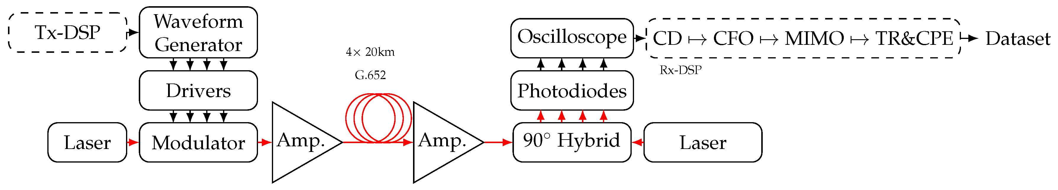
Figure 2.
Quantum circuit of the Bell-state measurement. The measurement is obtained by first transforming the Bell basis into the standard basis with and then measuring in the standard basis.
Figure 2.
Quantum circuit of the Bell-state measurement. The measurement is obtained by first transforming the Bell basis into the standard basis with and then measuring in the standard basis.
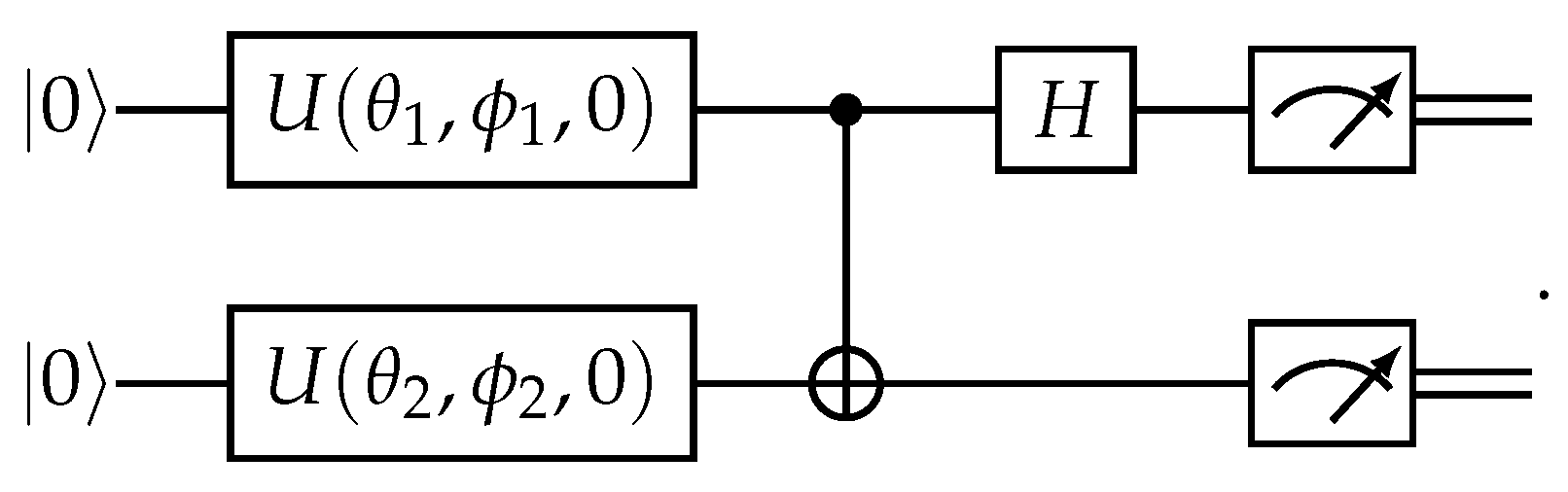
Figure 3.
Inverse Stereographic Projection (ISP) from [45] (left) and ISP with different radii (right).
Figure 3.
Inverse Stereographic Projection (ISP) from [45] (left) and ISP with different radii (right).
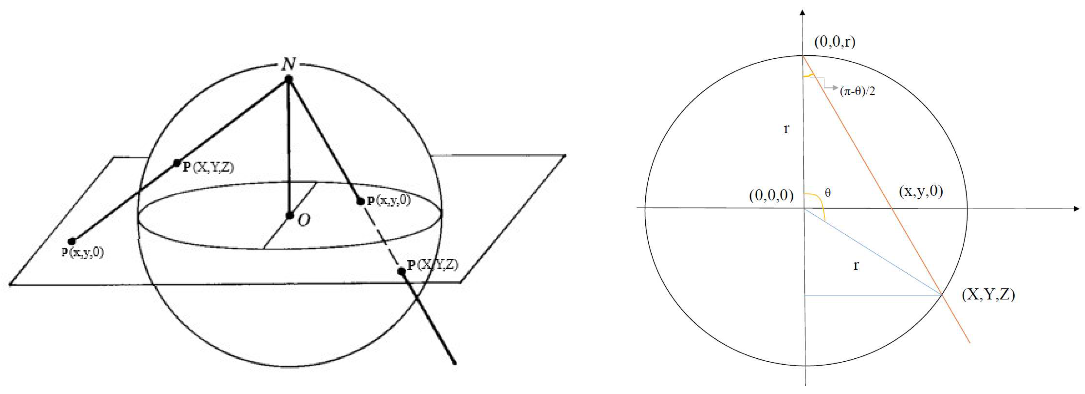
Figure 4.
A diagram providing a visual intuition for how the stereographic quantum k nearest-neighbour clustering quantum algorithm is equivalent to the 2DSC-kNN k nearest-neighbour clustering classical algorithm.
Figure 4.
A diagram providing a visual intuition for how the stereographic quantum k nearest-neighbour clustering quantum algorithm is equivalent to the 2DSC-kNN k nearest-neighbour clustering classical algorithm.
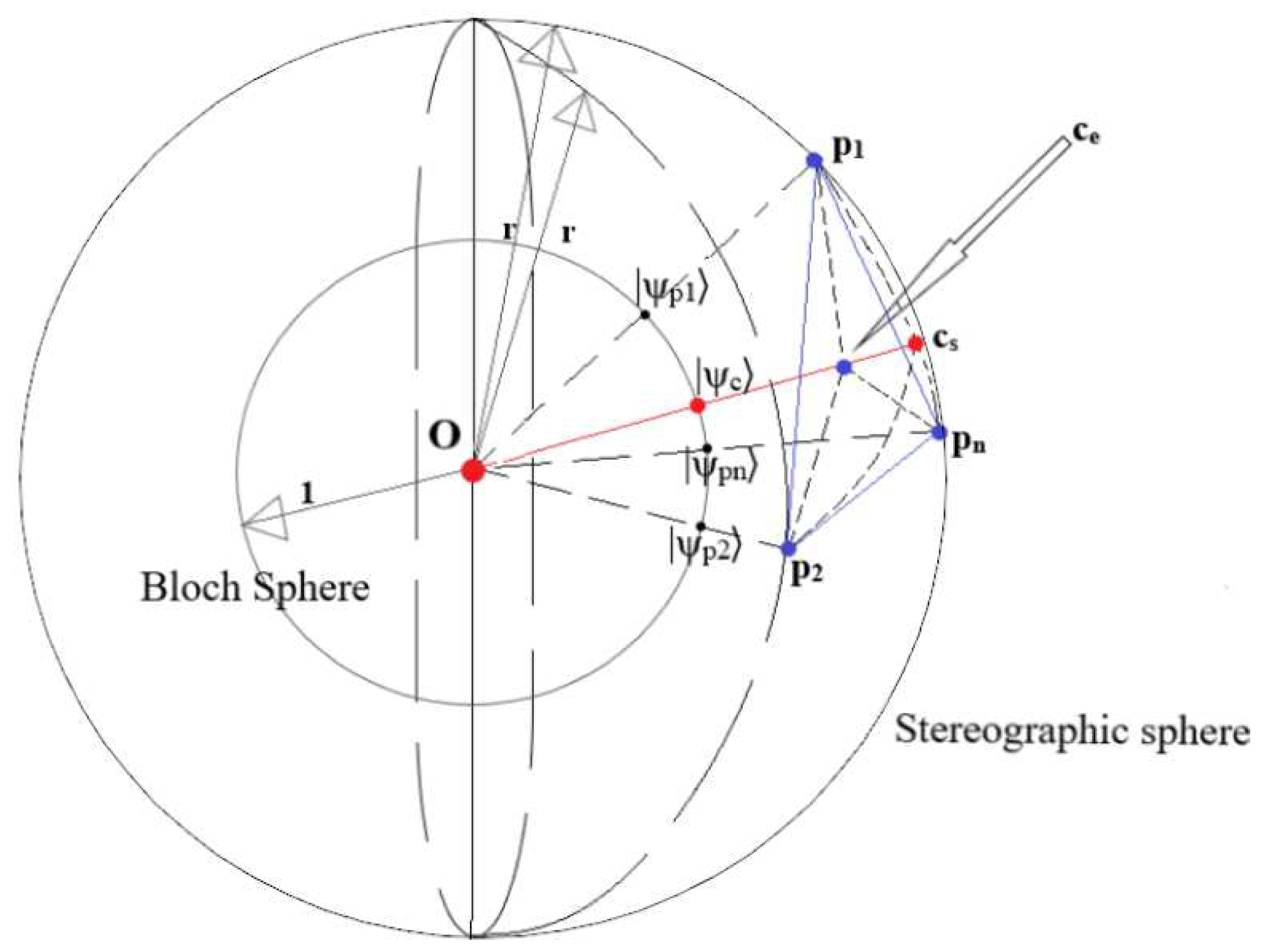
Figure 5.
Mean testing (top) and training (bottom) accuracy v/s ln(Number of points) v/s ln(projection radius) for the 2DSC-kNN algorithm acting upon the 2.7 dBm dataset. Full data on the left and a close-up on the right.
Figure 5.
Mean testing (top) and training (bottom) accuracy v/s ln(Number of points) v/s ln(projection radius) for the 2DSC-kNN algorithm acting upon the 2.7 dBm dataset. Full data on the left and a close-up on the right.
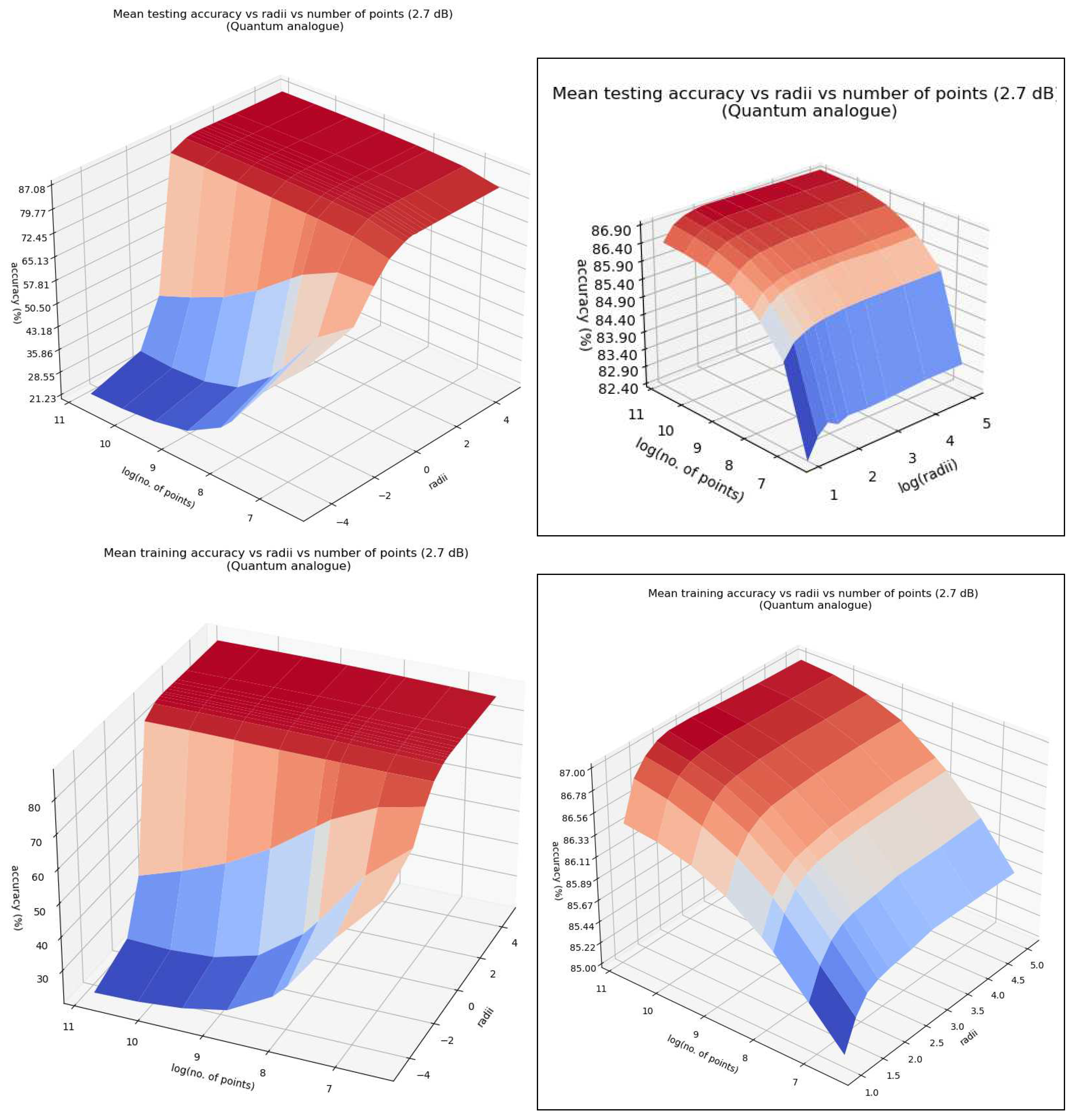
Figure 6.
Heat map of Mean accuracy v/s ln(Number of points) v/s projection radius for the 2DSC-kNN algorithm acting upon the 2.7 dBm dataset. Testing on the left, training on the right.
Figure 6.
Heat map of Mean accuracy v/s ln(Number of points) v/s projection radius for the 2DSC-kNN algorithm acting upon the 2.7 dBm dataset. Testing on the left, training on the right.
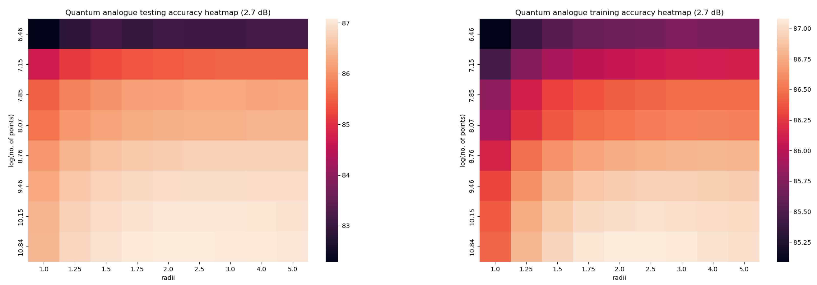
Figure 7.
Mean number of iterations in training v/s Number of points v/s log(projection radius) for the 2DSC-kNN algorithm acting upon the 10.7 dBm dataset. Two views on the top and a close up at the bottom.
Figure 7.
Mean number of iterations in training v/s Number of points v/s log(projection radius) for the 2DSC-kNN algorithm acting upon the 10.7 dBm dataset. Two views on the top and a close up at the bottom.
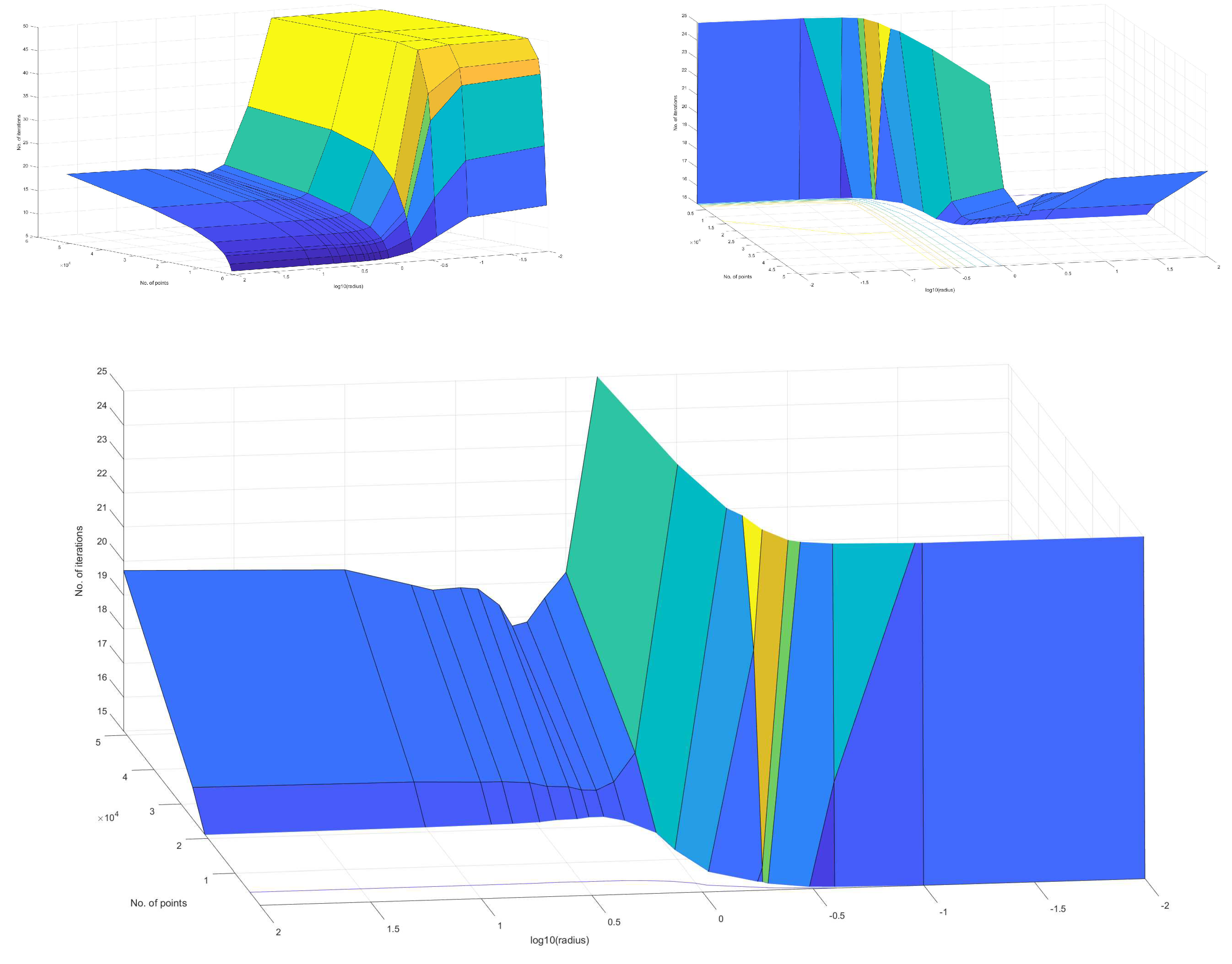
Figure 8.
Mean testing accuracy (top) and accuracy gain (bottom) v/s the natural log of the number of points for the 2.7 dBm (left) and 10.7 dBm (right) datasets.
Figure 8.
Mean testing accuracy (top) and accuracy gain (bottom) v/s the natural log of the number of points for the 2.7 dBm (left) and 10.7 dBm (right) datasets.
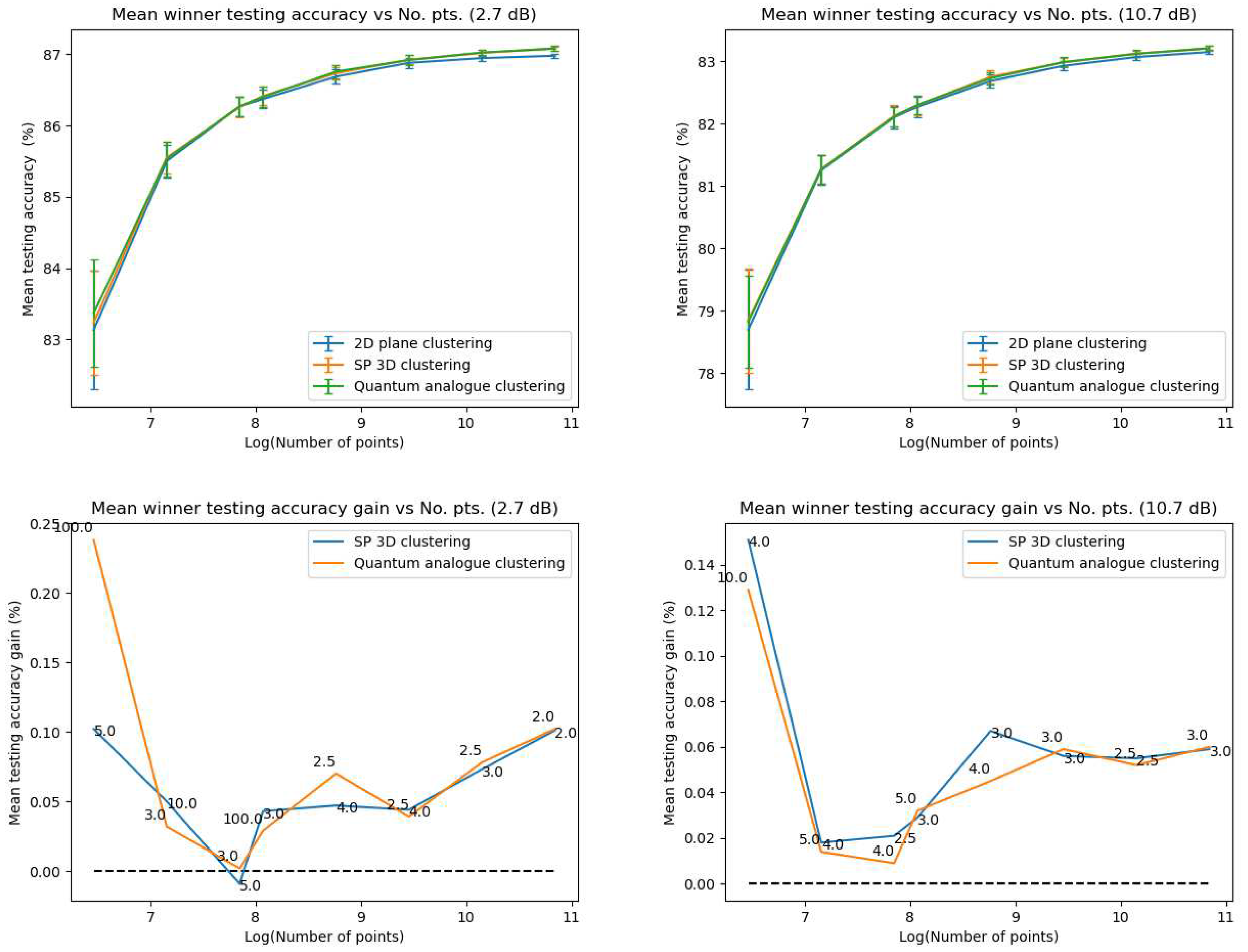
Figure 10.
Mean training iterations (top) and iteration gain (bottom) v/s the natural log of the number of points for the 2.7 and 10.7 dBm datasets.
Figure 10.
Mean training iterations (top) and iteration gain (bottom) v/s the natural log of the number of points for the 2.7 and 10.7 dBm datasets.
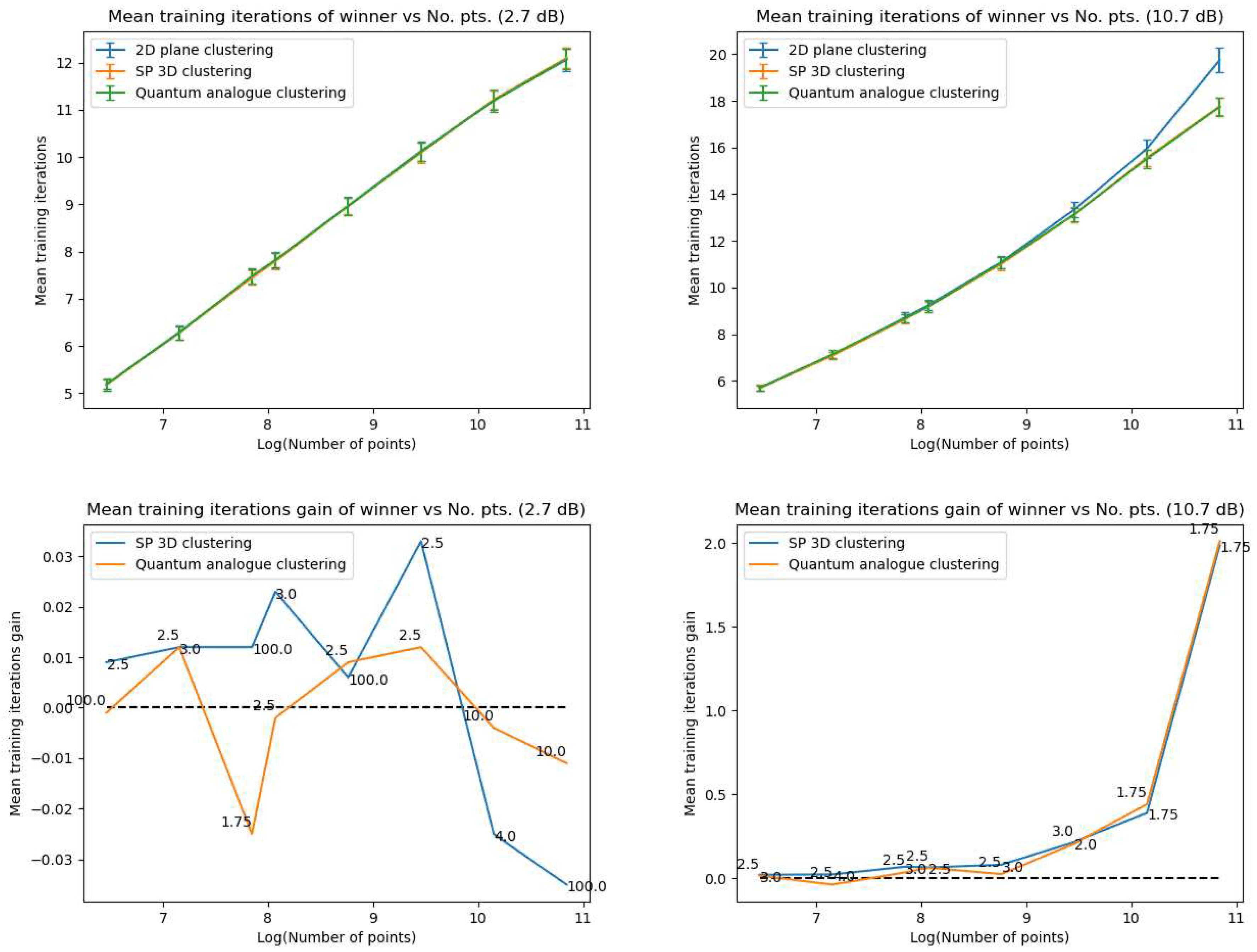
Figure 11.
Mean testing (top) and training (bottom) execution time v/s the logarithm of the number of points for the 2.7 dBm (left) and 10.7 dBm (right) datasets.
Figure 11.
Mean testing (top) and training (bottom) execution time v/s the logarithm of the number of points for the 2.7 dBm (left) and 10.7 dBm (right) datasets.
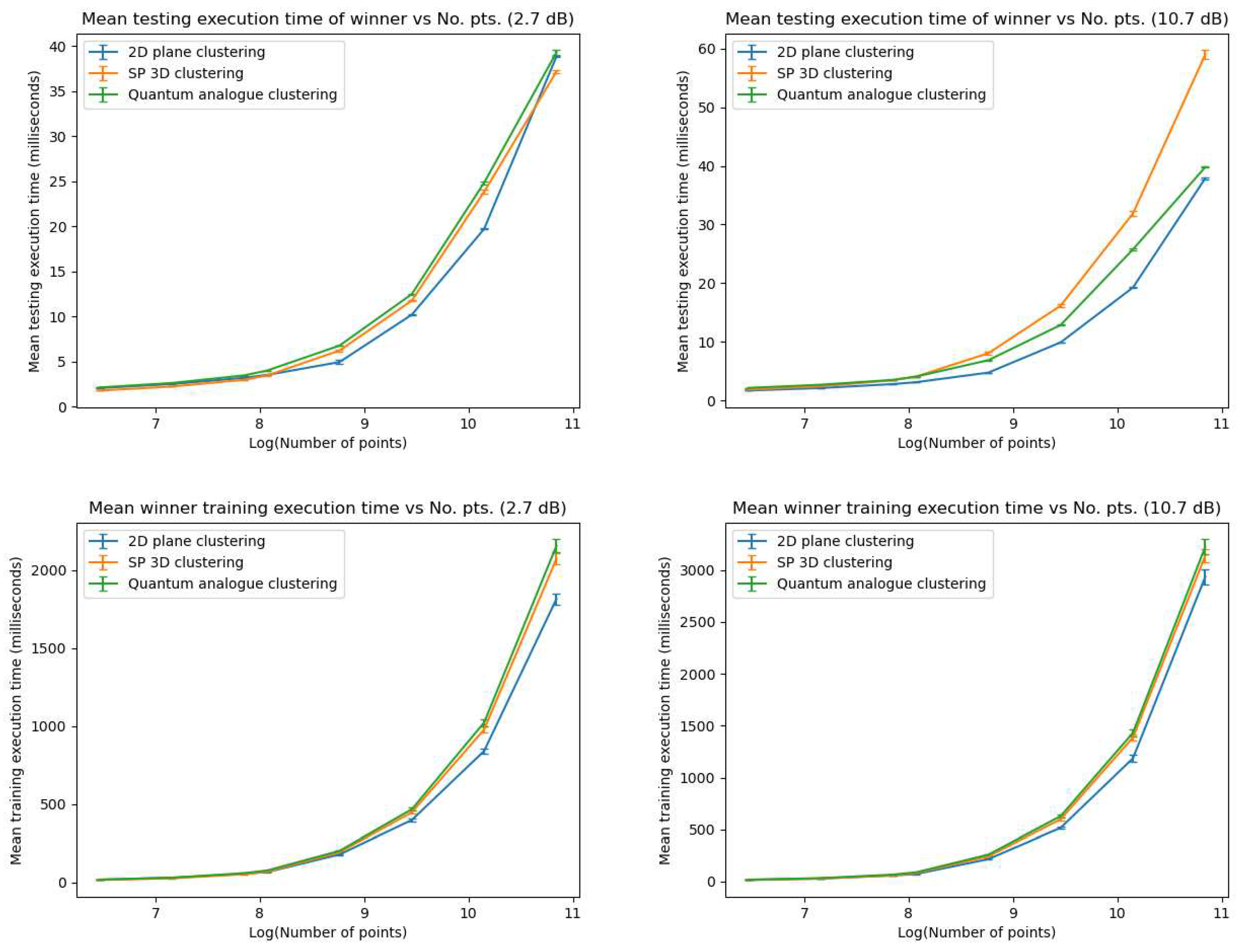
Figure 12.
Mean testing (top) and training (bottom) execution time gain v/s the logarithm of the number of points for the 2.7 dBm (left) and 10.7 dBm (right) dataset.
Figure 12.
Mean testing (top) and training (bottom) execution time gain v/s the logarithm of the number of points for the 2.7 dBm (left) and 10.7 dBm (right) dataset.
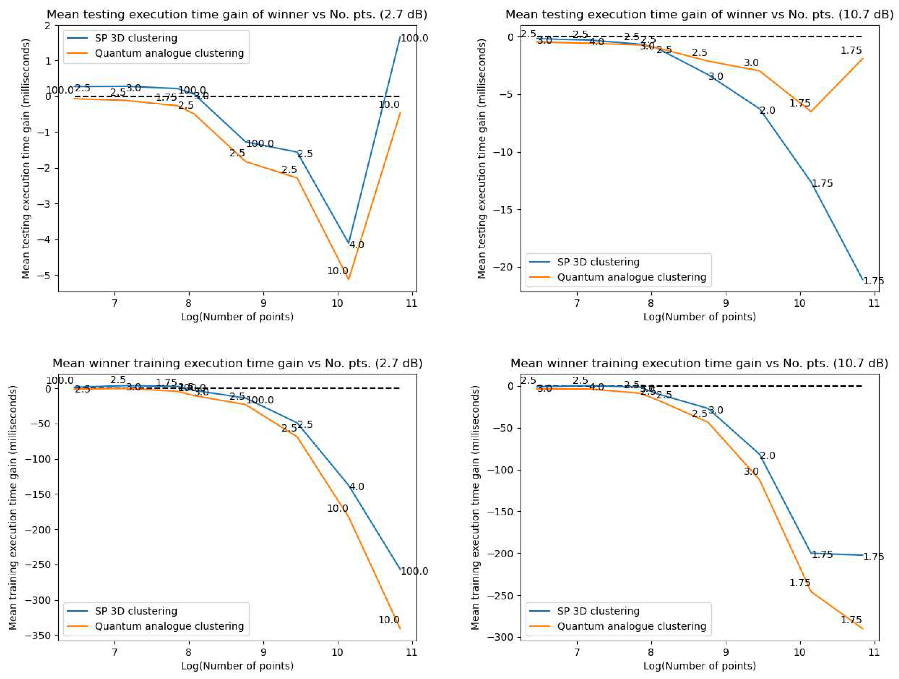
Figure 13.
Mean overfitting parameter v/s the natural log of the number of points for the four datasets.
Figure 13.
Mean overfitting parameter v/s the natural log of the number of points for the four datasets.
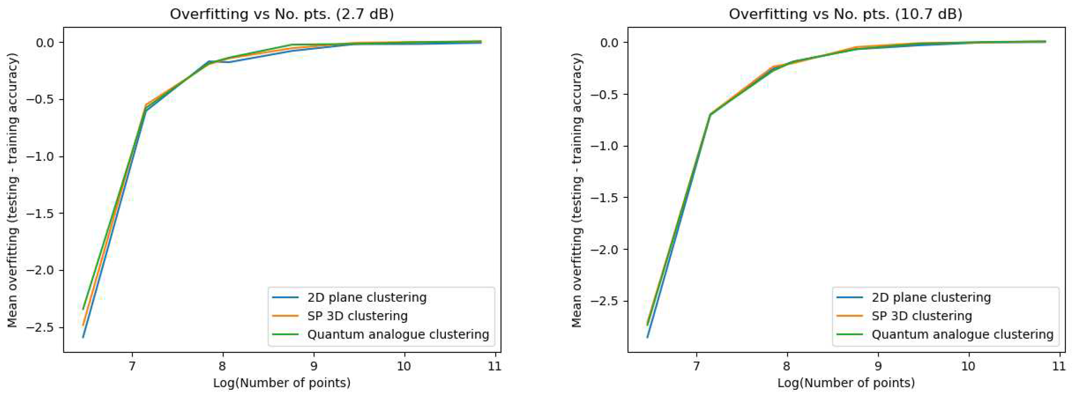
Figure 14.
Maximum Accuracy v/s iteration number v/s projection radius for the 2DSC-kNN algorithm acting upon the 2.7 dBm dataset. Close-up of the maximas at the bottom.
Figure 14.
Maximum Accuracy v/s iteration number v/s projection radius for the 2DSC-kNN algorithm acting upon the 2.7 dBm dataset. Close-up of the maximas at the bottom.
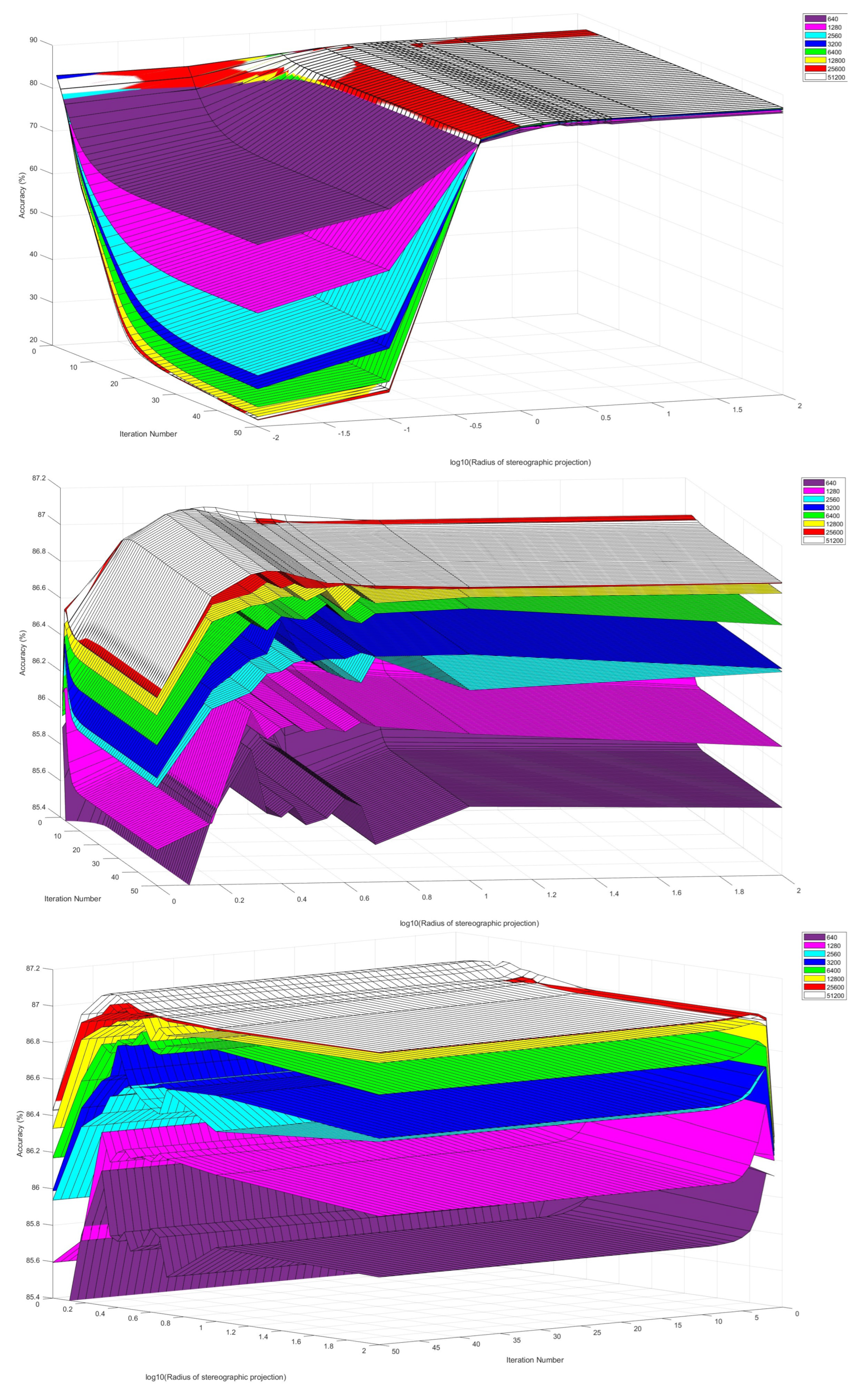
Figure 15.
Probability of stopping v/s projection radius v/s iteration number for 2DSC-kNN algorithm. Top: 2.7 dBm dataset with the number of points = 640. Bottom: 10.7 dBm dataset with the number of points = 51200.
Figure 15.
Probability of stopping v/s projection radius v/s iteration number for 2DSC-kNN algorithm. Top: 2.7 dBm dataset with the number of points = 640. Bottom: 10.7 dBm dataset with the number of points = 51200.
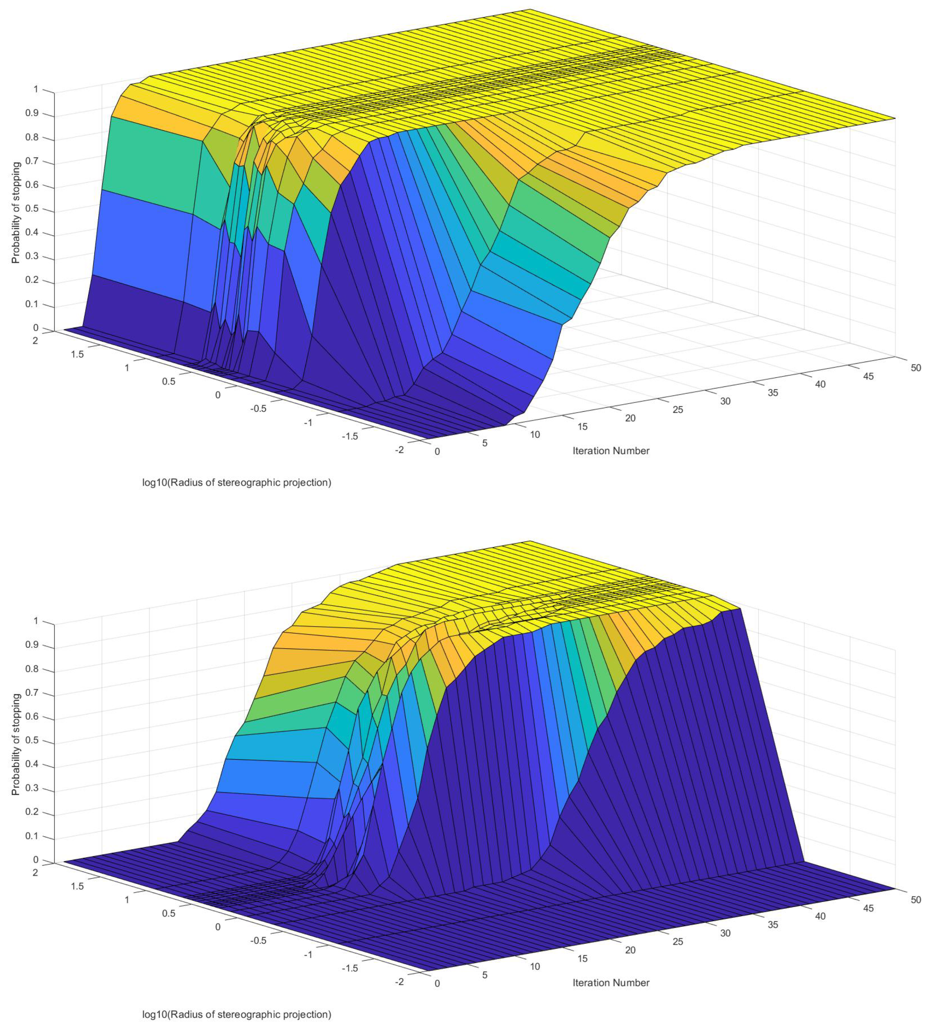
Figure 16.
Gain in iteration number at maximum accuracy (number of iterations at maximum accuracy of 2DEC-kNN minus the number of iterations at maximum accuracy of 3DSC-kNN (blue) and 2DSC-kNN (red)) v/s number of points for the 2.7 dBm (left) and 10.7 dBm (right) datasets.
Figure 16.
Gain in iteration number at maximum accuracy (number of iterations at maximum accuracy of 2DEC-kNN minus the number of iterations at maximum accuracy of 3DSC-kNN (blue) and 2DSC-kNN (red)) v/s number of points for the 2.7 dBm (left) and 10.7 dBm (right) datasets.
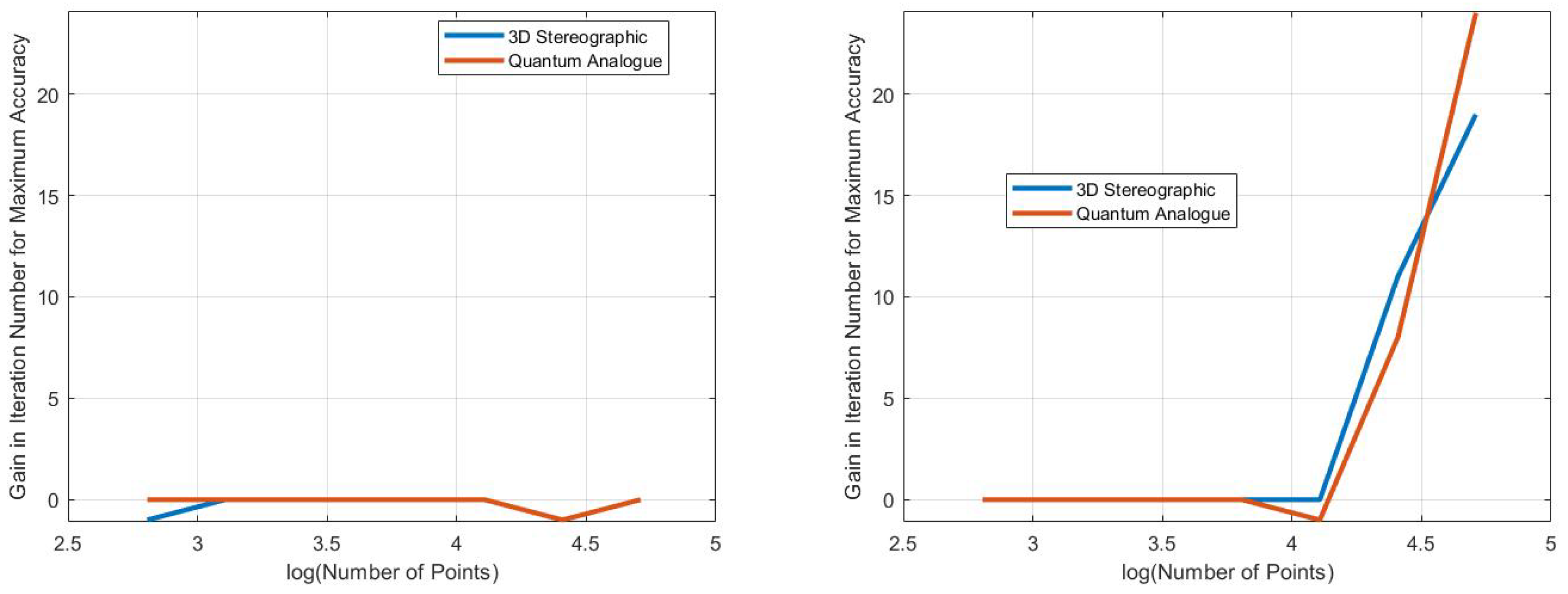
Figure 17.
Gain in maximum accuracy of 2dSC-kNN (red) and 3DSC-kNN (blue) algorithms v/s number of points for the 2.7 dBm (left) and 10.7 dBm (right) datasets.
Figure 17.
Gain in maximum accuracy of 2dSC-kNN (red) and 3DSC-kNN (blue) algorithms v/s number of points for the 2.7 dBm (left) and 10.7 dBm (right) datasets.
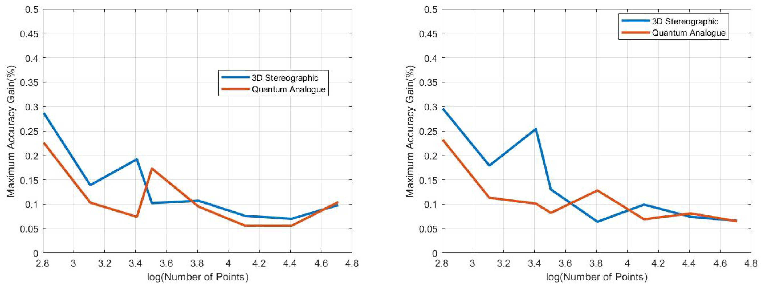
Figure 18.
Maximum accuracy of 2dSC-kNN (red), 3DSC-kNN (blue) and 2DEC-KNN (yellow) algorithms v/s number of points for the 2.7 dBm (left) and 10.7 dBm (right) datasets.
Figure 18.
Maximum accuracy of 2dSC-kNN (red), 3DSC-kNN (blue) and 2DEC-KNN (yellow) algorithms v/s number of points for the 2.7 dBm (left) and 10.7 dBm (right) datasets.
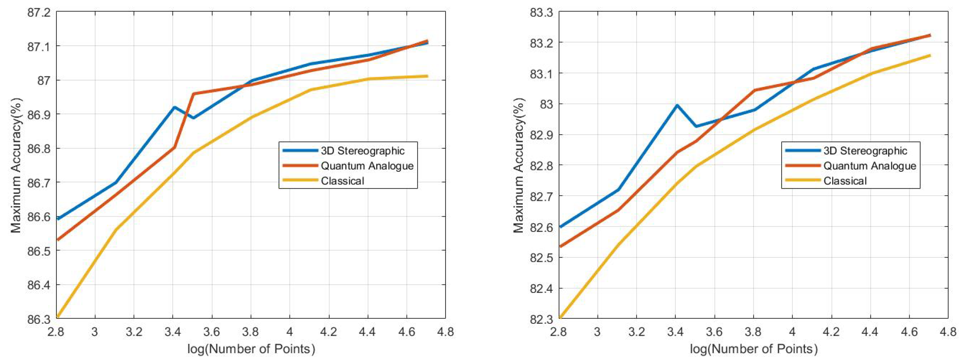
Table 1.
Summary of various kNN algorithms, where SC stands for “stereographic classical” (2D or 3D) and SQ for “stereographic quantum”. Here, D is the 2-dimensional dataset, are the 2-dimensional initial centroids (initial transmission points), is the ISP into , and the dissimilarities , and are defined in Equation (25) and Definitions 5 and 8, respectively. The option of using instead of in the 2DSC-kNN is due to Remark 3.
| Algorithm | Reference | Dataset | Initial | Dataspace | Dissimilarity | Centroid |
| Centroids | Update | |||||
| D | d | |||||
| 2DEC-kNN | Definition 4 | D | ||||
| 3DSC-kNN | Definition 6 | |||||
| 2DSC-kNN | Definition 12 | (or ) | ||||
| SQ-kNN | Definition 10 |
Disclaimer/Publisher’s Note: The statements, opinions and data contained in all publications are solely those of the individual author(s) and contributor(s) and not of MDPI and/or the editor(s). MDPI and/or the editor(s) disclaim responsibility for any injury to people or property resulting from any ideas, methods, instructions or products referred to in the content. |
© 2023 by the authors. Licensee MDPI, Basel, Switzerland. This article is an open access article distributed under the terms and conditions of the Creative Commons Attribution (CC BY) license (http://creativecommons.org/licenses/by/4.0/).
Copyright: This open access article is published under a Creative Commons CC BY 4.0 license, which permit the free download, distribution, and reuse, provided that the author and preprint are cited in any reuse.


