Delimitation of Ecological Corridor Using Technological Tools

Preprint

Article

Delimitation of Ecological Corridor Using Technological Tools

Altmetrics

Downloads

225

Views

Comments

A peer-reviewed article of this preprint also exists.

Submitted:

23 April 2023

Posted:

24 April 2023

You are already at the latest version

Alerts

Abstract

Ecological corridors function as a viable way to mitigate the environmental impact arising from forest fragmentation by interconnecting forest fragments through various techniques. In this context, the objective of this study is to propose a route for the implementation of an ecological corridor in the Itapemirim river watershed. The specific objectives were: (i) to delimit the permanent preservation areas (APP) of the Itapemirim river watershed and compare land use and land cover in the delimited areas; (ii) to calculate landscape ecology indices and select the forest fragments with the highest potential for ecological corridor implementation using Fuzzy logic; (iii) to assess costs and trace the best route for ecological corridor implementation, considering distance and physical impediments; (iv) to assess land costs and expropriation costs to delimit the ecological corridor in the study area. To map land use and land cover, the MapBiomas platform was used, based on Landsat 8 satellite images. The permanent preservation areas were delimited according to criteria established by Law No. 12.651 of May 25, 2012, which establishes parameters, definitions, and limits for APP. The characterization and structural quantification of some landscape ecology indices were performed using the QGIS 3.26 computational application, through the LecoS 3.0.1 plugin and Fragstats 4.2. The connected forest fragments were the Caparaó National Park, the Serra das Torres State Natural Monument, and the fragments selected through the application of Fuzzy logic to the landscape ecology indices. The corridor was delimited according to the lowest cost route, considering land use and land cover, APP, fragment potential, slope, and subnormal clusters. For each cost raster image, its respective statistical weights were calculated using the Analytic Hierarchy Process (AHP) hierarchical method, as well as for the analysis of priority areas for forest restoration, considering land use and land cover, APP, pedology, lithology, and biological importance. The interconnection between protected areas and fragments with the ecological corridor followed the orientation described by CONAMA nº 09/96. Based on the development of the work, the following results were identified: the highest land use and land cover class is pasture. Of the area designated for permanent preservation, 68.58% is in conflicting use with the legislation. The bare land value per hectare of the pasture class is the second highest among the bare land value per LULC values, representing 64.28% of the total. The priority area map showed that 31.86% of the area was classified as of very high or high importance and 42.97% as low or very low priority for forest restoration. Thus, it is concluded that the least cost path algorithm associated with the result generated by the multi-criteria decision method (AHP) constitutes an important tool for planning and implementing an ecological network by taking into account the primary factors for decision-making regarding the location of the best route.

Keywords:

Subject: Environmental and Earth Sciences - Ecology

1. Introduction

The Itapemirim River basin (BHRI) is one of the main ones in Espírito Santo, with an area of approximately 5,946 km² (594,599.095 ha). This watershed encompasses lands from the states of Minas Gerais (0.55% of its area) and Espírito Santo (99.45% of its area), and has various degrees of degradation due to territorial occupation marked mainly by livestock and coffee farming [1], as well as marble and granite mining industries [2,3].

The basin is fully located in the Atlantic Forest [4], with its remaining forest fragments assuming fundamental importance for maintaining the biome. The loss of natural forests, combined with a more recent process of intensification of fragmentation, has resulted in landscapes with little diversity of natural habitats [5].

One of the consequences of forest fragmentation is the loss of genetic diversity, caused by the reduction of natural ecosystem areas [6,7]. In addition, it increases the risks of inbreeding and favors the establishment of invasive species [8]. Fragmentation affects not only species but also the entire landscape structure, with implications for essential ecosystem services for maintaining biodiversity and human populations, such as climate regulation, air quality, changes in the hydrological regime, watershed flooding and siltation, soil erosion, floods, and epidemics [9,10,11].

In this way, ecological corridors can generate improvements in environmental services and the quality of natural resources, since they can be formed by forest and agroforestry systems, with economic returns to benefit both wildlife and local community residents [12].

Ecological corridors (EC) function as a viable way to mitigate the environmental impact resulting from forest fragmentation, through the interconnectivity of forest fragments, through different forms [13,14]. Some authors and environmental protection organizations recognize the importance of adopting corridors for landscape connectivity, through the restoration of biodiversity, reducing the risks of species extinction and maintaining the resilience of ecosystems in various parts of the planet [15,16,17,18].

It is important to consider spatial factors in the implementation of ecological corridors in a hydrographic basin, such as the distance between fragment edges, optimal paths for fauna translocation, distance to water bodies, availability of water in quality and quantity, and the presence of physical barriers such as roads and cities [19]. Some studies have shown that the paths chosen by animals between forest fragments take into account cost-benefit considerations, such as the presence of food, ground cover, and topographical obstacles [20].

One method to support the creation of ecological corridors across the landscape is the Least-Cost Path Analysis (LCP) algorithm, using Geographic Information Systems (GIS) [21]. Through LCP analysis, it is possible to determine the optimal flow route between two points within a cost matrix, which are assigned based on previously established criteria [18,22,23].

In addition to the LCP method, Fuzzy logic [24,25] corresponds to an extension of Boolean logic, which allows for flexibility in models that involve uncertainties regarding acceptable or unacceptable limits, acceptable and not acceptable, it allows for intermediate values between true and false, being suitable for problems that do not have well-defined boundaries [26].

The fuzzy concept has been implemented in various fields of knowledge with convincing results, such as mapping flood susceptibility [17] and developing fire risk maps [27,28]. Therefore, this study aims to benefit the Itapemirim River hydrographic basin through the implementation of ecological corridors, as it can bring a better use directly to the biota, as there is greater efficiency in the environmental management of protected areas, as well as benefits to the soil and water resources in the surrounding areas.

2. Materials and Methods

2.1. Characterization of the study area

The hydrographic basin of the Itapemirim river (BHRI) is located in the state of Espírito Santo (ES), Brazil, between latitudes 20°9’36’’ and 21°7’12’’ South and longitudes 40°46’13.08’’ and 41°52’19.92’’ West, with an area of 6,181 km² (Figure 1). It covers the municipalities of Alegre, Atílio Vivácqua, Castelo, Conceição de Castelo, Cachoeiro de Itapemirim, Itapemirim, Iúna, Irupi, Ibatiba, Jerônimo Monteiro, Marataízes, Muqui, Muniz Freire, Presidente Kennedy, Vargem Alta, Venda Nova do Imigrante, and part of the municipality of Lajinha in the state of Minas Gerais [29].

Two main types of climate are identified in the BHRI, namely subtropical highland climate with dry winter and mild summer (Cwb), with average temperatures below 22º C, subtropical with dry winter (with average temperatures below 18º C) and hot summers (with temperatures above 22º C) (Cwa), and tropical, with rainy season in the summer from November to April, and dry season in the winter from May to October (Aw) [30].

2.2. Database

2.2.1. Land use land cover (LULC)

The overall accuracy was obtained by MapBiomas (2020), (Table 1), where a cross-tabulation of sample frequencies of the mapped classes was performed. A sample evaluation of pixels, composed of approximately 75,000 samples, was conducted, in which the number of samples is pre-established by statistical sampling techniques, using metrics that compare the mapped class with the class evaluated by technicians in the reference database.

For the analysis of land use and land cover changes (LULC) (Table 1), the LULC data from MapBiomas for the year 2021, collection 7.0, with a spatial resolution of 30 m and annual temporal resolution, were used. The images were exported from the Google Earth Engine cloud platform and processed using QGIS software version 3.26.

MapBiomas is a dataset that provides annual dynamics of land use and land cover (LULC) in Brazilian biomes, where annual maps are produced from pixel-by-pixel classification of Landsat satellite images. The processing is done using machine learning algorithms through the Google Earth Engine platform [31,32]. The choice of the year 2021 is based on the characteristics of the satellite type, as the most recent collection was released from this period. The use of MapBiomas product is driven by its availability, accessibility, and applicability with pre-classified data.

The class of paved/unpaved roads described in Frame 1 was obtained through download from the open-source OpenStreetMap application, which contains paved and unpaved roads at a global level. These roads are generated through civilian use of the application.

The first step was to define the projection of the roads for compatibility with the Land Use and Land Cover (LULC) data, as well as delineate the watershed and conservation units. Subsequently, the selection of roads within the watershed area was performed, and a buffer of 15 meters on each side was created, totaling a width of 30 meters for paved/unpaved roads. This value does not represent the reality, as paved roads typically have an average width of 10 meters. However, a value of 30 meters was adopted due to the working scale, where the other LULC classes were generated with 30-meter pixels. The final step involved converting the vector data to raster, with cells of 30 meters, and updating this class in the LULC data.

2.3. Delimitation of permanent preservation areas (APP)

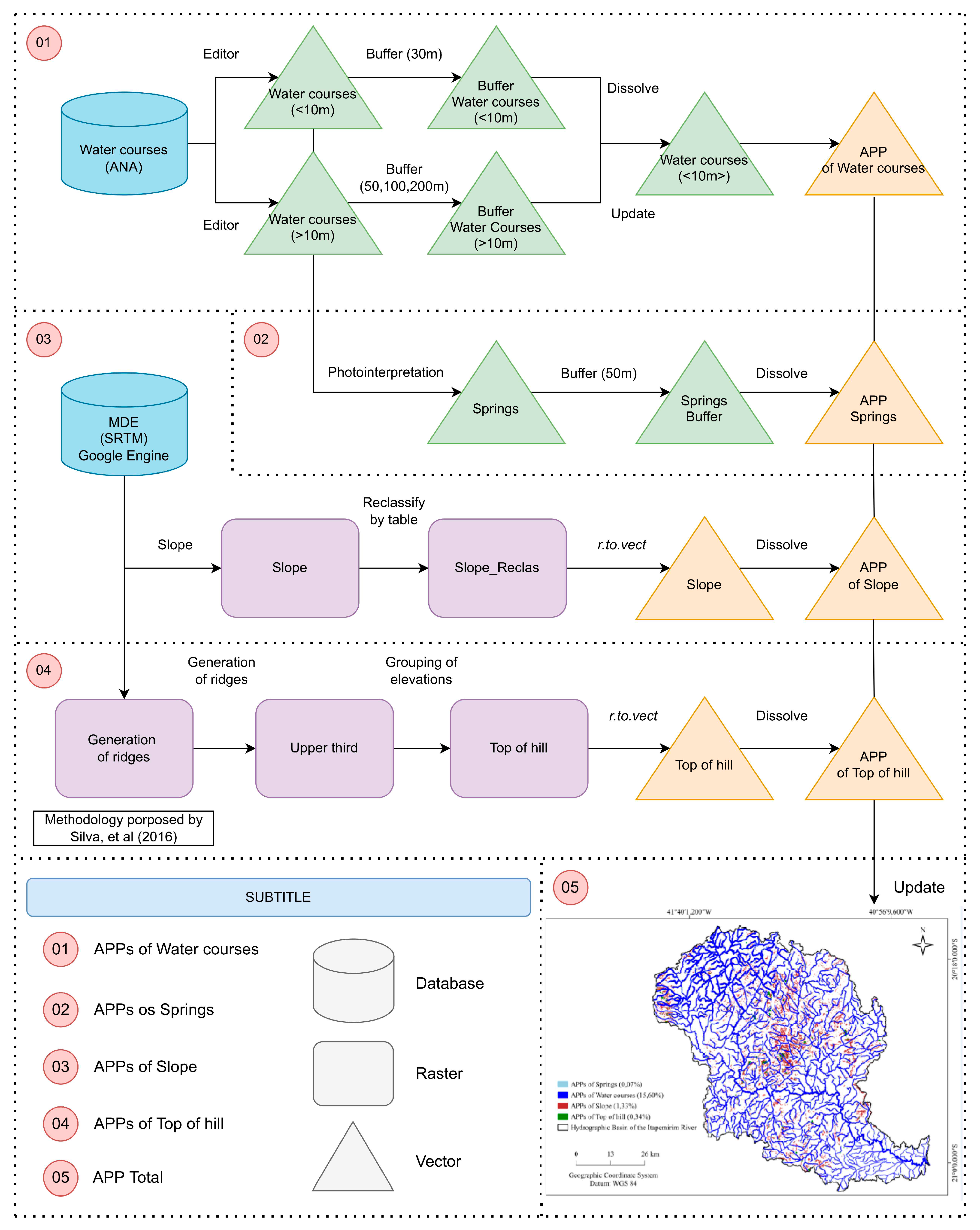
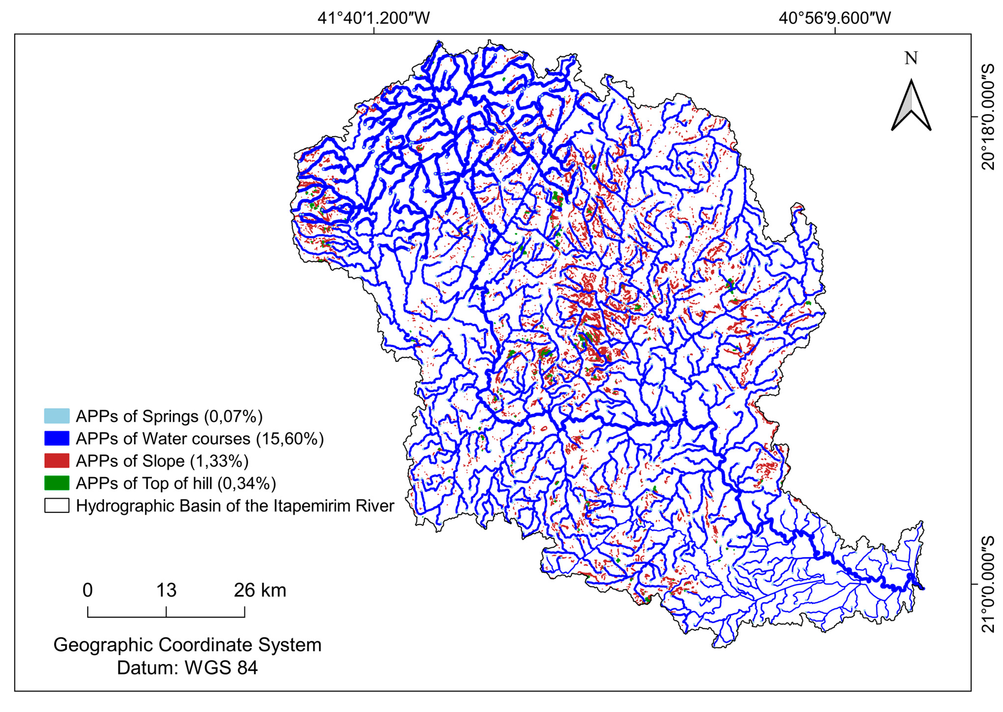
For the delimitation of APP, four classes were considered (Frame 2), according to the criteria established by Law No. 12,651 of May 25, 2012, which establishes criteria, definitions, and limits of APPs [33]. All methodological steps for mapping the APPs were carried out in the QGIS software, version 3.26, and are presented in Figure 2.

• Mapping of APP for watercourses:

For watercourses, the "buffer" command was applied to delimit buffer zones of 30 meters on each side, considering that during the rainy season, the width of each watercourse does not exceed 10 meters. However, the BHRI has watercourses that exceed 10 meters in width during the rainy season, and to map them, it was necessary to use land use and land cover data.

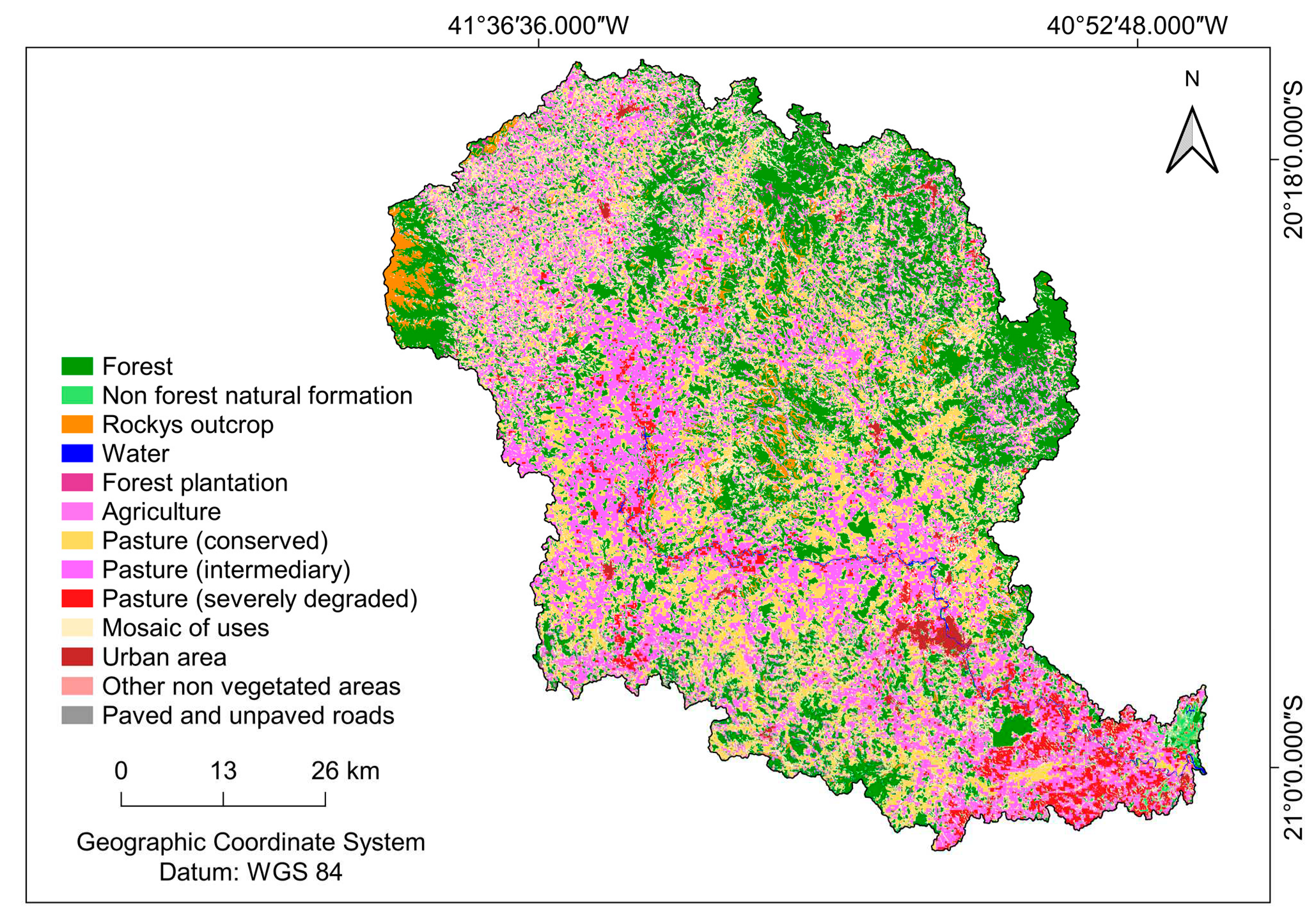
After obtaining the land use and land cover data for the BHRI, the Water Bodies were imported in polygonal format, and the Water Bodies class was edited to remove polygons of lakes, lagoons, reservoirs, among others. This allowed for the selection of polygons that delimit watercourses, where each segment with a width greater than 10 meters was re-applied the "buffer" command according to the width as per Table 3. Subsequently, the "union" command was applied after using the "buffer" command of 30 meters on the watercourses with different categories mentioned in Table 3, generating the final Watercourse APP results.

Table 2. Damping width to be used for APP generation according to the width of the water courses.

Width of the watercourse (meters)	Damping width for APP generation (meters)
30, 40 e 50	50
60, 80, 90, 100 e 190	100
220, 240 e 550	200

• Mapping of the APP for springs:

The springs were manually marked using the QGIS version 3.26 editor, based on the hydrography generated in the previous step. Each watercourse beginning was marked with a point, generating a point vector containing 576 springs. After this step, the "buffer" command available in QGIS version 3.26 was executed to delimit a 50-meter preservation radius around each of the springs, resulting in the delineation of the APP of springs.

• Mapping of the APP of slope:

Using the SRTM (Shuttle Radar Topography Mission) elevation data, specifically SRTM V3 provided by NASA, the Digital Elevation Model (DEM) of the study area was reprojected and added to QGIS version 3.26, where slope values of the BHRI (Base Hidrográfica do Rio Itapemirim) were calculated. Subsequently, slope values were classified, assigning NoData to slopes less than 45 degrees and a value of 1 to slopes greater than this threshold. The resulting raster from this processing was converted to vector, generating the APP of slope.

• Mapping of the APP of top of hill:

The methodology of Silva et al. (2016) was used within the QGIS software version 3.26, and it involves several steps, from image acquisition to obtaining the APP zones, including:

1. Download of SRTM scenes for the study área;

2. Removal of elevation values >= 1800 meters using the "Raster Calculator" tool;

3. Execution of the "r.fill.dir" algorithm to fill spurious depressions in the Digital Elevation Model (DEM) and obtain the Hydrologically Consistent Digital Elevation Model (HCDEM).

4. Inversion of the HCDEM using the following equation, executed via the "Raster Calculator", and obtaining the raster "mdehc_inv":

hcdem_inv = (HCDEM – 10000)*(-1)

5. Execution of the "r.terraflow" algorithm on the "mdehc_inv" raster to obtain the limits of the peaks’ base, resulting in the output raster "limite_bases";

6. Conversion of "limite_bases" to vector format, keeping the same name;

7. Execution of the "Zonal Statistics" tool, using the "limite_bases" vector on the "hcdem" raster. This tool calculates maximum, minimum, mean, range, and other values within the raster, considering the limits of the vector. Output: "zonal_statistics_hcdem";

8. Calculation of the slope, in degrees, from the "hcdem" raster. Output raster: "slope";

9. Execution of the "Zonal Statistics" tool, using the "limite_bases" vector on the "declividade" raster. This aims to obtain the average slope for each area. Output: "zonal_statistics_slope";

10. Selection and extraction of average slopes >= 25 degrees (from the "zonal_statistics_declividade");

11. Calculation of the range in the "zonal_statistics_hcdem" layer (adding the "amplitude" column):

amplitude = altitude_max - altitude_min

Note: after the execution of "Zonal Statistics", the "range" column can be used as equivalent to amplitude, as it represents the difference between the maximum and minimum values.

12. Selection and extraction of features where the value of "amplitude" >= 100 m;

13. Identification of areas where slope >= 25 degrees and amplitude >= 100 m using the "extract by location" tool, predicate "equal";

14. Calculating the minimum height for the upper third: adding a column "terco" to the previously extracted layer (item 13):

terco = altura_maxima - (amplitude/3)

15. Rasterizing the resulting layer from the previous step, using the column "terco" as the output value (output raster: "min_alt_terco"). This procedure can be done using the "v.to.rast" algorithm;

16. Extracting from "hcdem" the pixels where the values are greater than or equal to "min_alt_terco". Output: "app_topofhill";

17. Vectorizing "app_topofhill", exporting only the pixels with value = 1. Output: "app_topofhill_final".

• Mapping of the APP total:

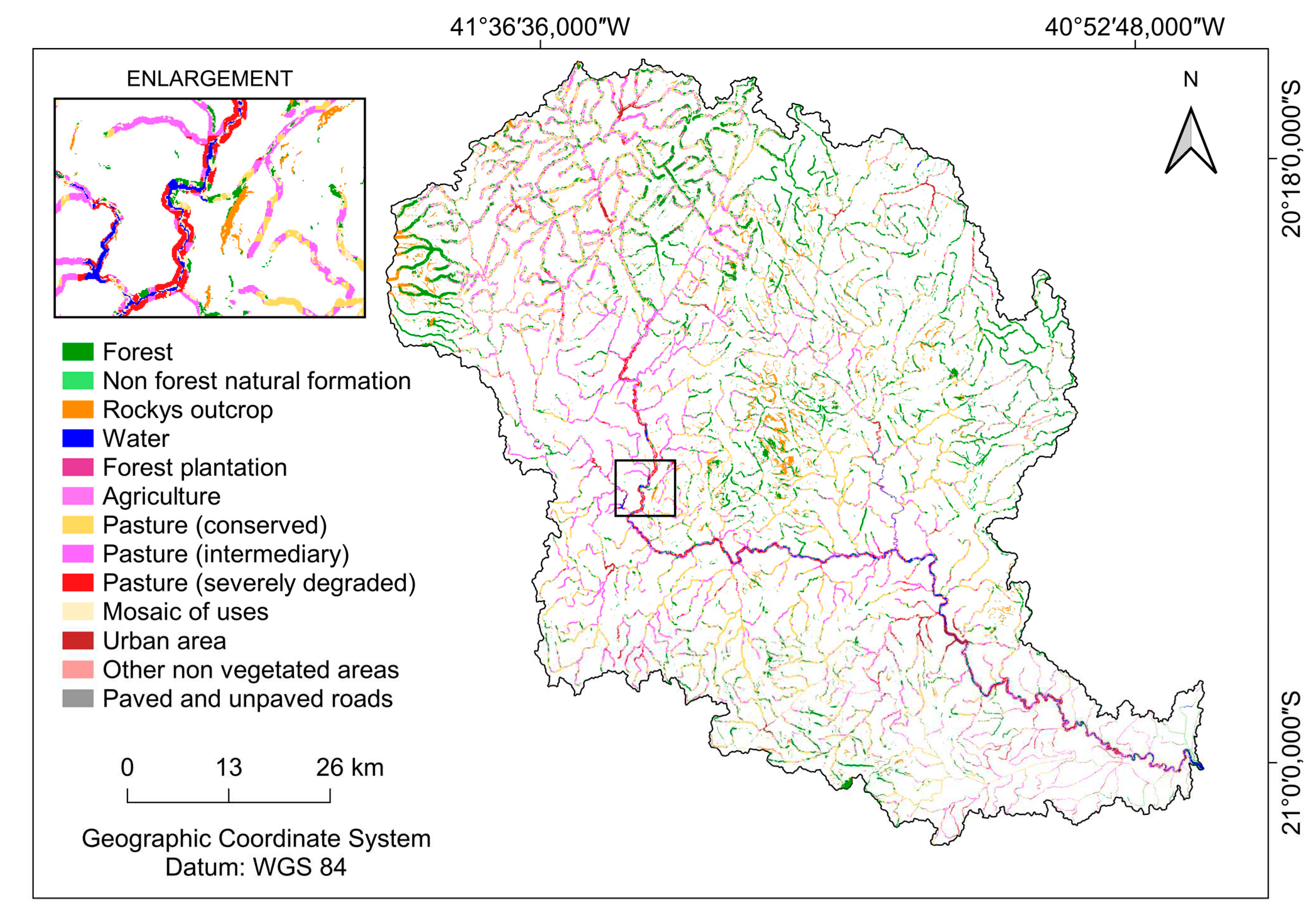
The map of the total APP of BHRI was generated by grouping the data acquired individually from each of the four APP classes. The tabular cross-tabulation technique was used to quantify and determine the percentage of each land use and land cover class in the APP total, through map overlay.

2.4. Comparison of land use and land cover with permanent preservation areas (APP)

The comparison between the thematic maps of LULC and the APP was carried out through the "clip" tool for analysis of the APP total in QGIS version 3.26. The classes of Forest, Non-forest natural formation, Rocky outcrop, and Water bodies were considered as suitable land use and land cover (non-conflicting) because these are natural land use and land cover classes, while the other classes were considered conflicting with the forest code.

2.5. Selection of forest fragments based on landscape ecology metrics índices

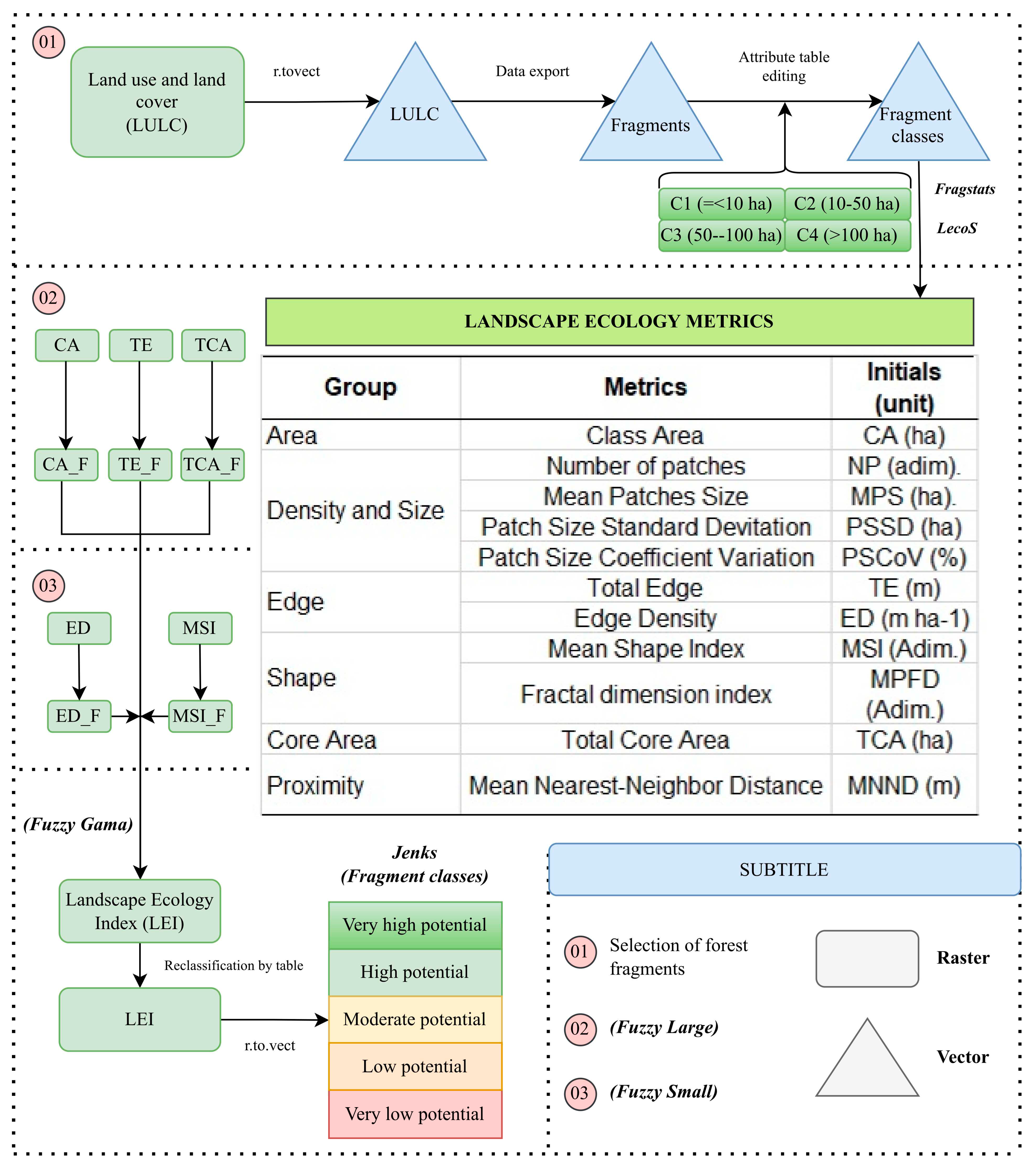
The characterization and evaluation of forest landscape ecology metrics were performed using the QGIS software version 3.26, Fragstats 4.2, and the LecoS plugin 3.0.1, as depicted in Figure 3.

2.5.1. Landscape ecology metrics indices

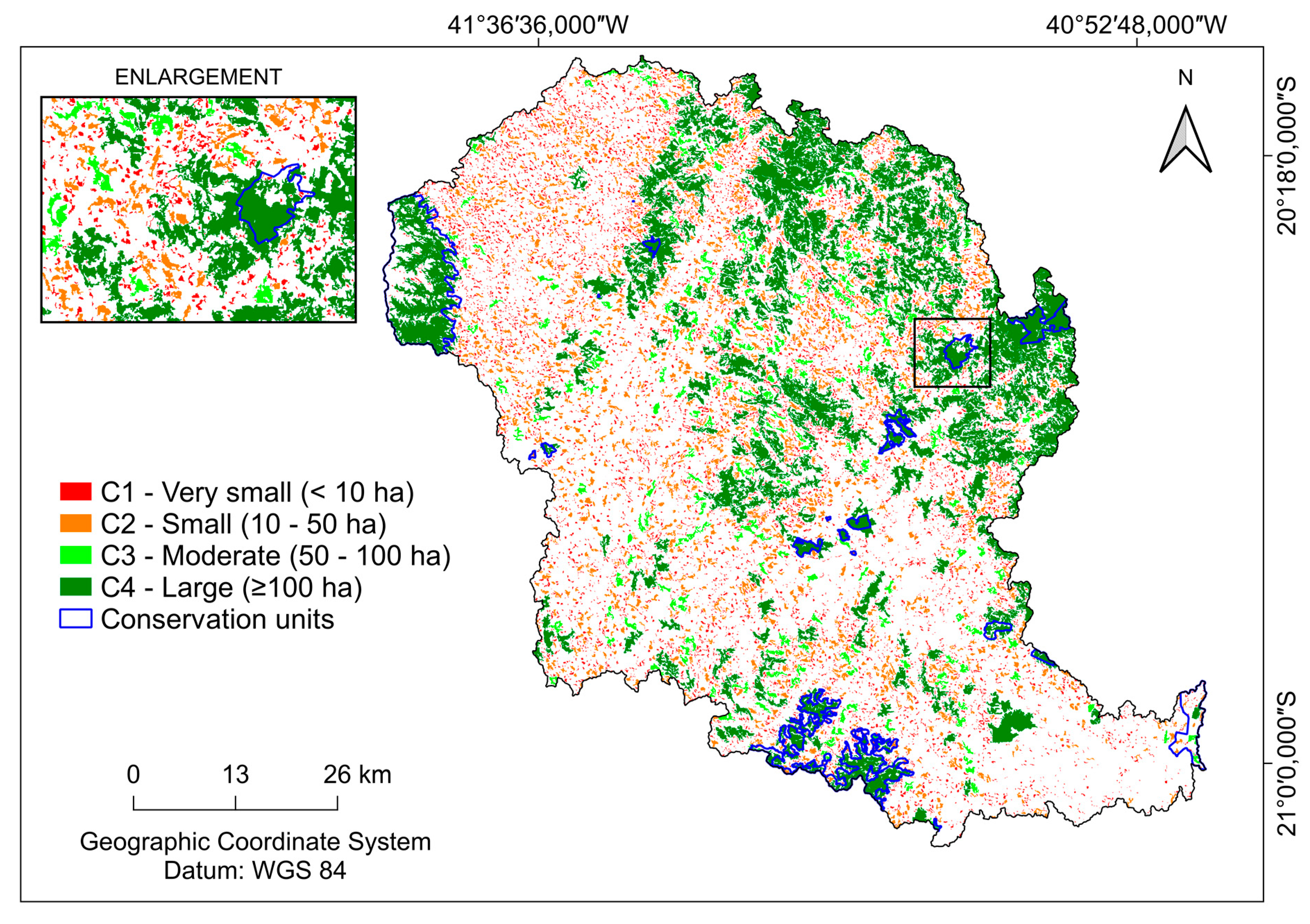
The polygons of forest fragments were selected from the land use and land cover map obtained from previous steps, resulting in a vector file of forest fragments. In order to compare conservation indices, the fragments were grouped based on their area, following the classification proposed by Santos et al. (2018), as very small (C1 < 10 ha), small (10 ≤ C2 < 50 ha), moderate (50 ≤ C3 < 100 ha), and large (C4 ≥ 100 ha). A buffer distance of 100 meters was adopted for measuring central area metrics (COUTO-SANTOS; CONCEIÇÃO; FUNCH, 2015). The metrics used for quantifying landscape structure are described in Frame 3.

The equations for landscape metrics used are described in Mcgarigal and Marks (1995), Lang and Blashke (2007), and Peluzio (2017), for the respective groups, as follows:

• Area metrics: Refers to the sum of the areas of all fragments of the study class (Equation 1).

C A = \sum_{i = 1}^{n} c_{i}

(1)

Where,

CA: sum of the areas of all fragments that belong to a certain class, in hectares; and,

c_{i}

: area of the i-th fragment corresponding to the evaluated class, in hectares.

• Density and size metrics: Represented by a set of equations that determine the Total number of patches or classes under study (Equation 2), Mean patch size (Equation 3), Standard deviation of mean patch size (Equation 4), and Coefficient of variation of mean patch size (Equation 5).

N P = \sum^{​} n_{i}

(2)

M P S = \frac{\sum_{j = 1}^{n} a_{i j}}{n_{i}}

(3)

P P S D = \sqrt{\frac{\sum_{j = 1}^{n} | a_{i j} - (\frac{\sum_{j - 1}^{n} a_{i j}}{n_{j}}) | ²}{n_{j}}}

(4)

P S C o V = \frac{P S S D}{M P S} * 100

(5)

Where,

NP: total number of patches within the same class or landscape (dimensionless);

number of patches of a class, if NP is at the landscape level, or one patch if NP is at the class level (dimensionless);

MPS: mean patch size, in hectares;

area of the i-th patch in the j-th class, in hectares;

j: number of patches in the class (dimensionless);

PSSD: standard deviation of mean patch size, in hectares;

number of patches in the j-th class (dimensionless); and,

PSCoV: oefficient of variation of mean patch size, in percentage.

• Metrics of edge: were represented by the sum of the perimeter of Total edge (Equation 6) and the Relative edge density in relation to the study area (Equation 7).

T E = \sum_{j = 1}^{n} e_{i}

(6)

E D = \frac{T E}{C A}

(7)

Where,

TE: sum of all edges of class or landscape, in meters;

e_{i} :

edge (perimeter) of the i-th fragment, in meters;

ED: edge density, in meters per hectare; and,

CA: total area of the class, in hectares.

• Shape metrics: were represented by the Mean Shape Index (Equation 8), which equals 1 when the fragments are circular and increases with the irregularity of the shape of the class, and by the Fractal Dimension (Equation 9), where values approach 1 for shapes with simple perimeters and increase with the complexity of the shape of the class.

M S I = \frac{\sum_{j = 1}^{n} | \frac{0, 25 p_{i f}}{\sqrt{a_{i j}}} |}{n_{i}}

(8)

M P F D = \frac{2 * \ln (0, 25 p_{i j})}{l n a_{i n}}

(9)

Where,

MSI: mean shape index (dimensionless);

p_{i f} :

perimeter of the fragment, in meters;

a_{i j} :

area of fragment i in class j, in hectares;

J: number of fragments (dimensionless);

n_{i} :

number of fragments in the class (dimensionless); and

MPFD: mean fragment perimeter fractal dimension (dimensionless).

• Metric of central area: It was presented by the total central area (Equation 10), which is the sum of all central areas of the class.

TCA = \sum_{j = 1}^{n} a_{i j}

(10)

In which,

TCA: total central area, in hectares; and,

a_{i j} :

interior area of fragment ij, in hectares.

• Proximity metric: It was presented by the average distance to the nearest neighbor (Equation 11).

MNND = \frac{\sum_{j = 1}^{n} h_{i j}}{n_{i}}

(11)

Where,

MNND: mean nearest neighbor distance, in meters;

h_{i j} :

minimum distance from fragment ij to its nearest neighbor, in meters; and,

n_{i} :

number of fragments in class i that have a nearest neighbor (adimensional).

2.5.2. Selection of forest fragments using Fuzzy logic

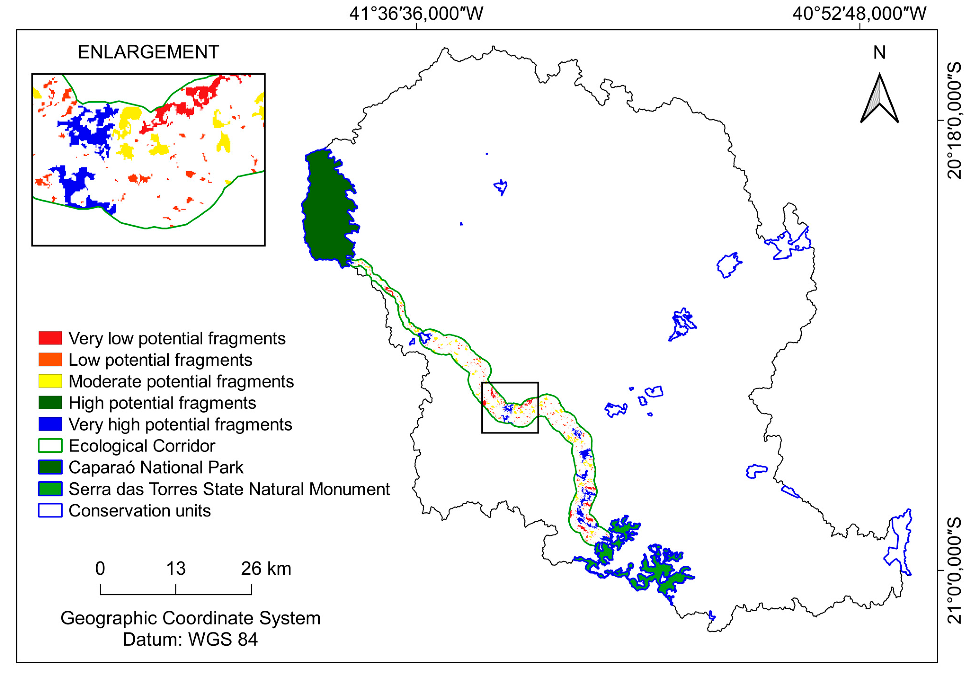
Were considered as having better preservation potencial, the fragments belonging to the “very high” class within the Fuzzy Gamma application.

The making of the database for the application of fuzzy logic was carried out in the computation applications Microsoft Excell® and QGIS 3.26. The database came from the previous methodological stage, using the metrics by fragmente and no longer by class. The landscape mtrics vectors área, border, shape and central area selected for characterization of the importance of the fragments were converted into a raster with a size of 30 meter cell. For each raster image, a pertinence function was defined with a degree of certainty that varies between “0 and 1”, in which the forest fragment with the highest degree of conservation and, consequently, the greatest potential for the passage of the ecological corridor was indicated when the real value of the variable assumes “1” and fragments with zero potential to integrate the ecological corridor were indicated when the real value of the variable assumes “0”, according to [26].

The structuring to be done with fuzzy logic allows a more realistic point of view when compared to other techniques due to its flexible description. There is less interference from the researcher, since the weight of each variable is not defined, but the maximum, average and minimum for the data to be accepted in the model [34].

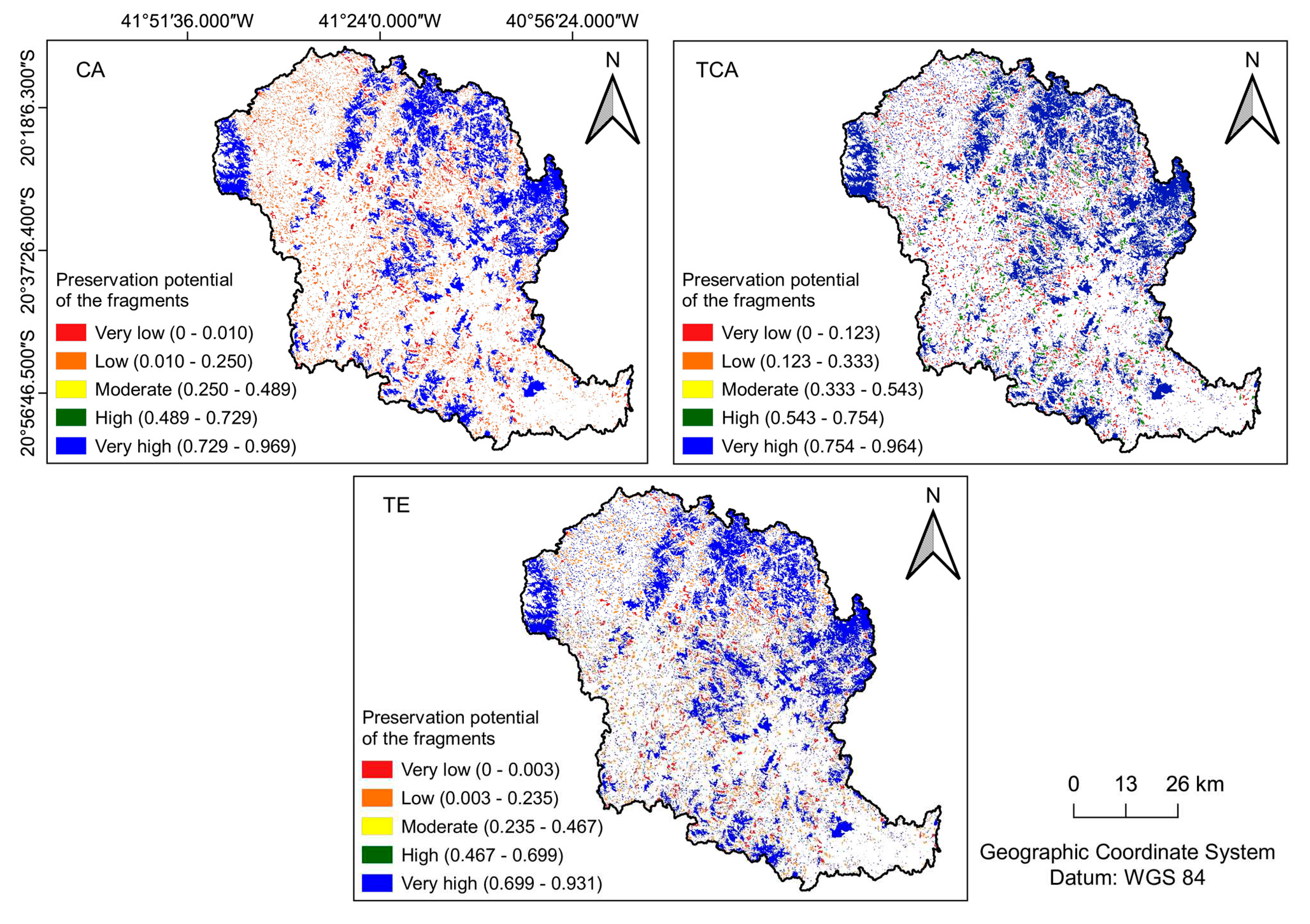
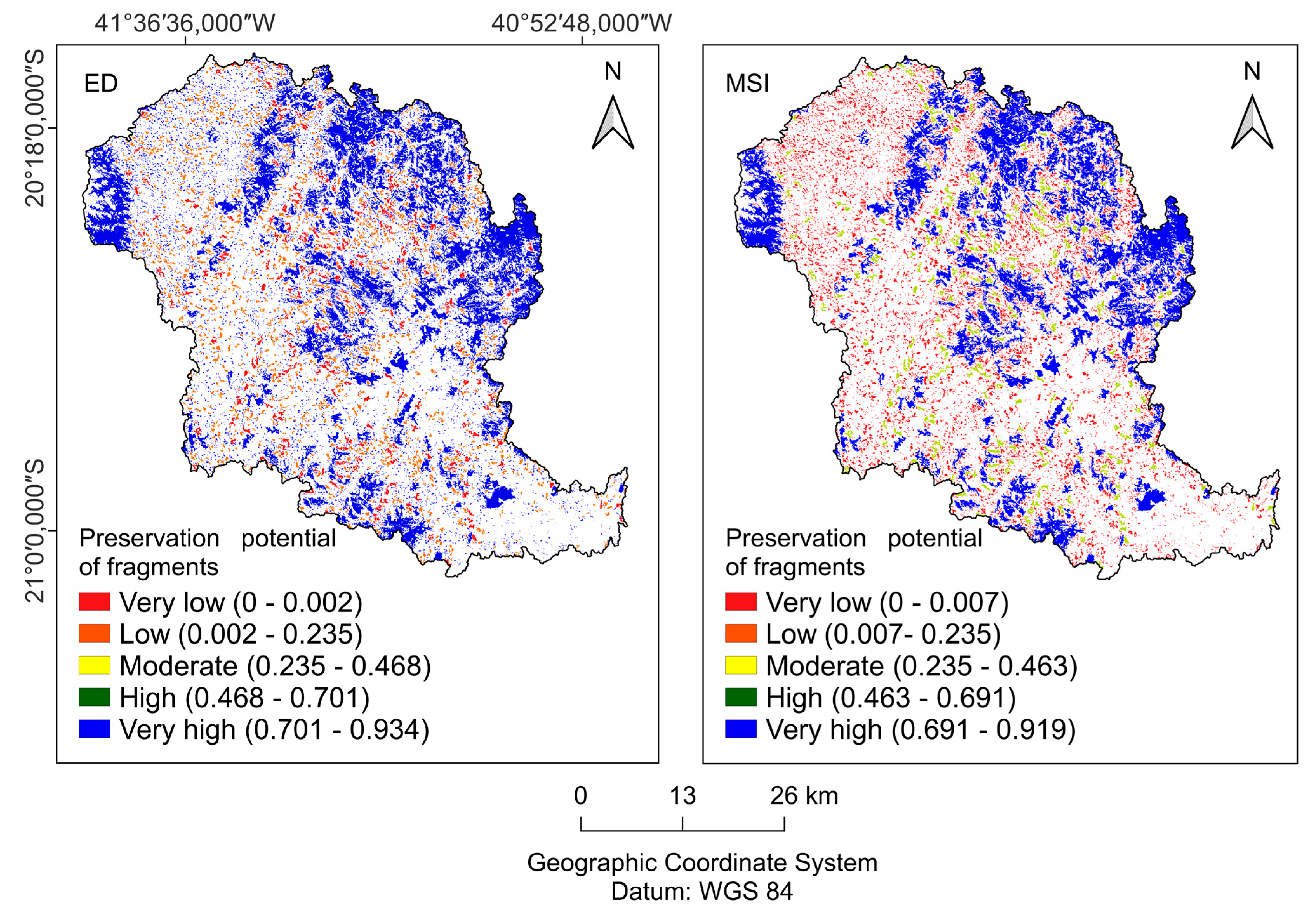
Metrics were selected by excluding redundant metrics and selecting representative metrics from the groups specified in Frame 3, with CA, TE, TCA, ED and MSI considered important for determining the degree of preservation of the fragments and, consequently, the relevance of adhesion of these fragments in the formation of EC.

For the CA, TE and TCA metrics, the increasing sigmoidal functions (Fuzzy Large) were adjusted for each fragment. This function makes it possible to represent the gradual variation around the matrix image, in which fragments that will come to be considered priority with larger area values have a greater chance of assuming a value of 1. The value to be defined at the central point was the one that confers a degree of relevance of 0.5 with a propagation value of 5, which defines the shape and characteristic of the transition zone (χ), expressed by Equation 12.

μ (X) = \frac{1}{1 + {(\frac{X}{c})}^{- a}}

(12)

Where,

μ(χ): corresponds to the degree of membership of the Large function from the variables;

a: parameter that determines the slope of the curve; and,

c: value at the midpoint where μ(χ) acquires 0.5.

The Fuzzy Small function was applied to the ED and MSI metrics, since for these variables, smaller input values will produce outputs closer to 1. The value defined at the central point was the one that gave a degree of membership of 0.5, with propagation value of 5, given Equation 13.

μ (X) = \frac{1}{1 + {(\frac{X}{c})}^{a}}

(13)

Where,

μ(χ): corresponds to the degree of membership of the Small function from the variables;

a: parameter that determines the slope of the curve; and,

c: value at the midpoint where μ(χ) acquires 0.5.

The Jenks optimization method, which has the spatial reclassification function, was applied to the matrix images of the metrics CA, TCA, TE, ED and MSI, generating the following classes of fragments: very high potential, high potential, moderate potential, low potential and very low potential.

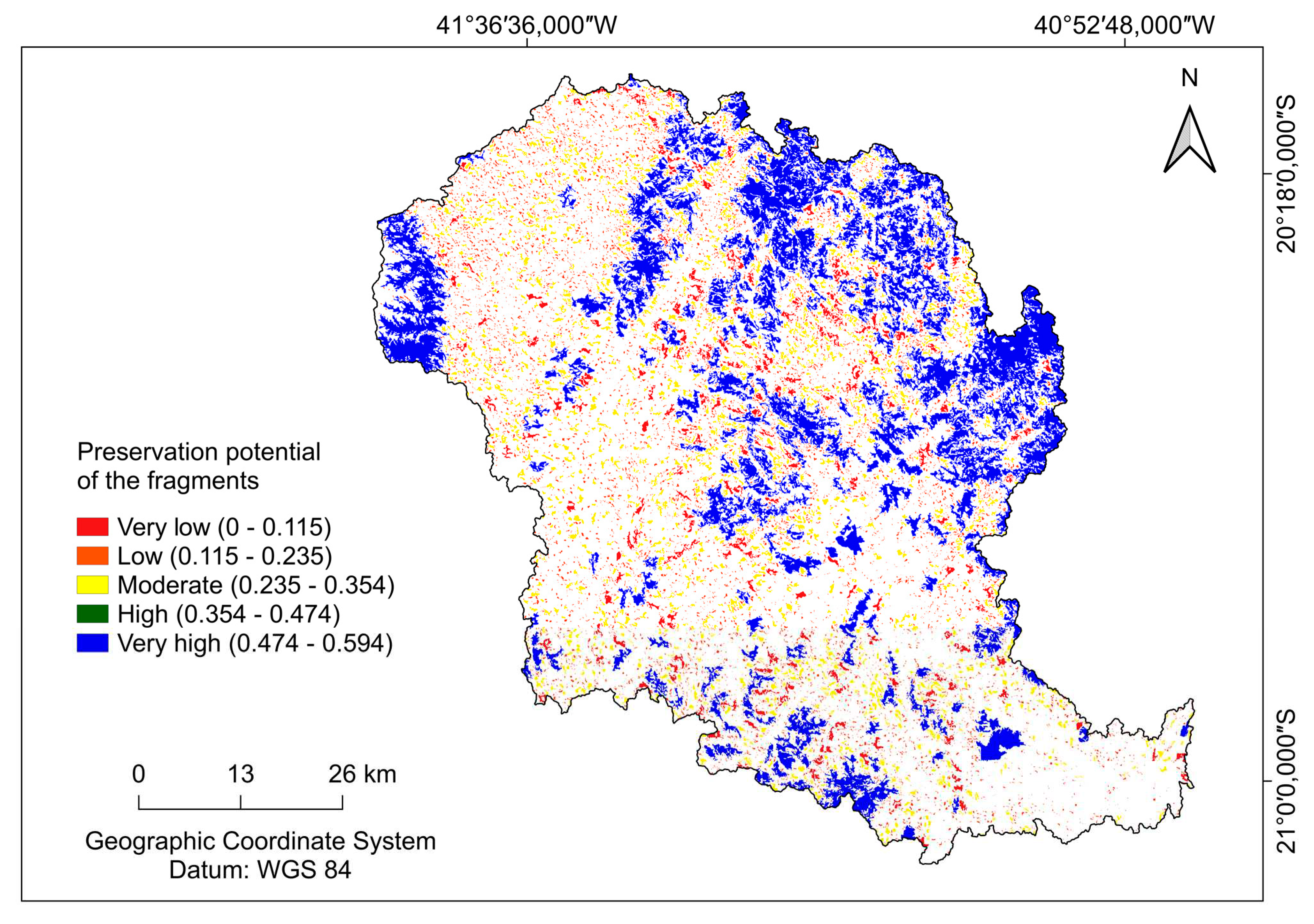
After the previous steps (Fuzzy small and Fuzzy large), Fuzzy Gamma was applied to combine the variables (CA, TE, TCA, ED and MSI). The Fuzzy Gamma operator makes it possible to handle a set of variables that have diffuse values through an overlay technique, in which it allows the increasing effect of the Fuzzy sum and the decreasing effect of the Fuzzy product to be combined [27,35]

As the objective of this stage is to select the fragments with the greatest potential for passing through the ecological corridor with values closer to 1, the value of the γ parameter used was 0.90, given by Equation 14.

μ (X) = {1 - \prod_{i - 1}^{n} (1 - μ_{i})}^{Y} * {\prod_{i - 1}^{n} μ_{i}}^{1 - y}

(14)

Where,

µᵢ: Fuzzy association values for i = 1, 2, ..., 5;

n: the raster data layer, that is, the number of variables in the study; and,

γ: a coefficient with values between 0 and 1.

The matrix resulting from the overlapping of variables was called the Landscape Ecology Index (LEI). Finally, the Jenks optimization method, which has the spatial reclassification function, was applied to the raster image resulting from the superimposition of variables (LEI), producing the following classes of fragments: very high potential, high potential, moderate potential, low potential and very low potential.

2.6. Delimitation of the ecological corridor (EC)

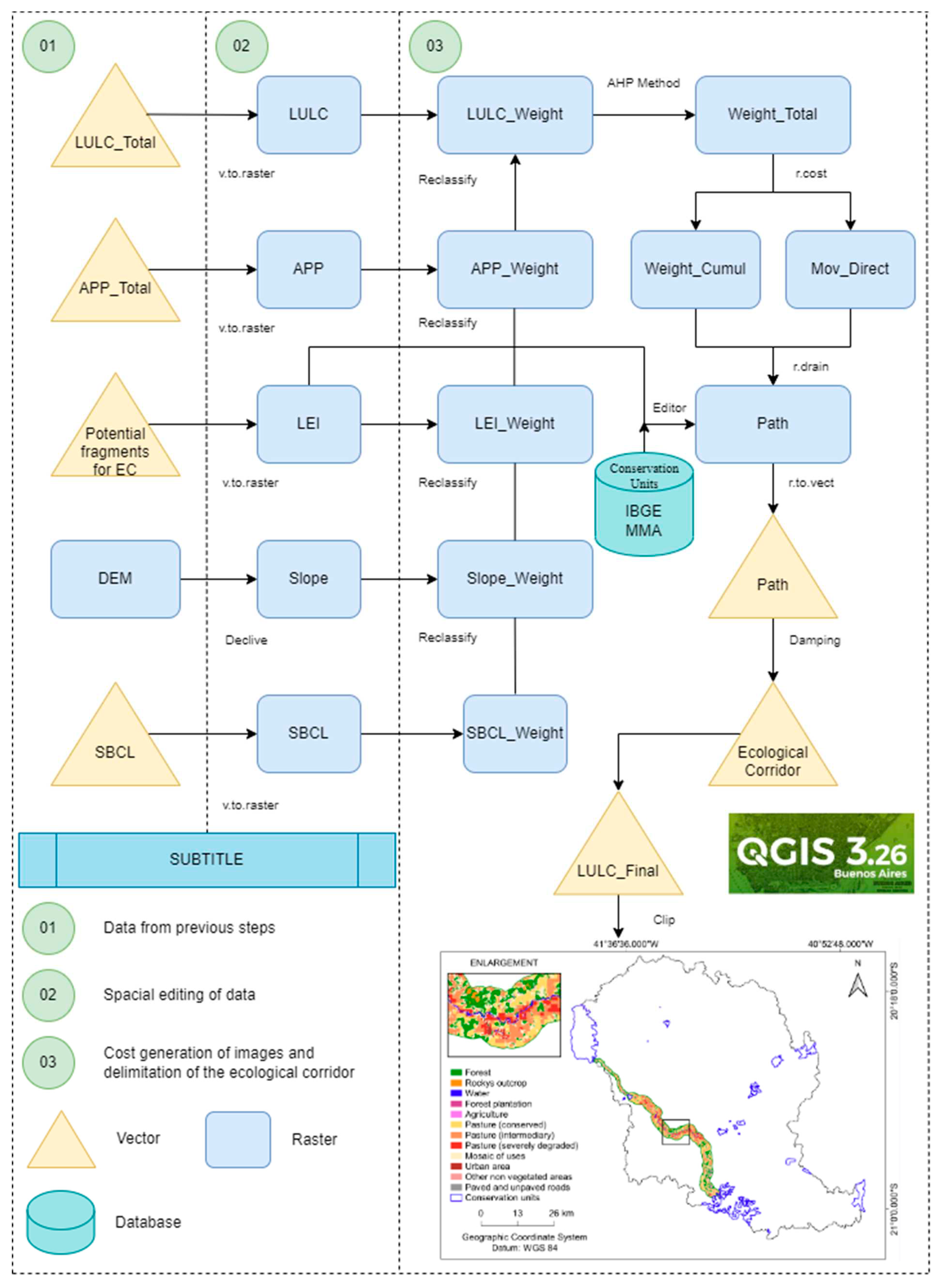
For the delimitation of the ecological corridor, an adaptation of the shortest course methodology, proposed by Santos et al (2022), was used, the width of the CE was established at 50% of the Brazilian resolution of CONAMA nº 09/96. The spatial basis used was derived from the previous steps, namely: a) boundary of the Itapemirim river basin, b) land use and occupation, c) permanent preservation areas defined in accordance with current Brazilian legislation, d) index of landscape ecology, e) digital elevation model, f) source polygon, Caparaó National Park, g) destination polygon, Serra das Torres State Natural Monument. In Figure 4 it is possible to visualize the flowchart containing the methodological steps used for the delimitation of the ecological corridor.

The choice of the UC, Caparaó National Park and Serra das Torres State Natural Monument, as a model area for the application of the methodology was made because both selected units have significant importance for the conservation of the region’s biodiversity, with the presence of endemic and endangered species. Caparaó National Park is known for housing Pico da Bandeira, the third highest point in Brazil, as well as remnants of Atlantic Forest and altitude fields. Serra das Torres State Natural Monument, on the other hand, is a conservation unit created with the objective of preserving a high-altitude cerrado area, also with rare and endangered species, which will allow for the evaluation of the effectiveness of ecological corridor proposals in the context of BHRI, contributing to conservation planning and management in the region.

For least cost path analysis, it will consist of determining the path of least resistance between two points (origin and destination). The resistance of each cell is represented by weights, based on some factor, or combination of factors, that affect the passage through the area.

Cost matrix images were generated, which represent some factor or combination of factors, as in the case of landscape metrics, which affect movement across an area. Costs will be defined in such a way as to prevent or limit the possibility of the corridor passing through undesirable areas such as built-up areas and roads. For each class, the suitability cost was determined, on a scale of 1 to 100, with the highest costs attributed to those where corridors should not pass, according to the different forms of use, giving rise to the friction map. Based on the UCT map, the costs were defined for each class, according to Moreira (2019), as shown in Frame 4. For Permanent Preservation Areas, springs, watercourses, slope and hill top, the complementary costs (SANTOS et al., 2022) (Table 3), in addition to areas of Subnormal Clusters (SBCL) (Table 4).

The selected forest fragments, through the analysis of the landscape ecology indices, received a cost value as follows (Table 5): very high potential received a cost of 1, since it generates a matrix image that allows the passage of the corridor through such areas, very low potential received cost 20, which makes the passage of the corridor in this area less interesting than in areas containing fragments of very high potential, but no less interesting than areas of forestry. The costs attributed to the different classes of forest fragments were based on the association of these classes with the land use and land cover costs in Frame 4.

The slope map was obtained using a 30m SRTM image, divided into three classes, namely: low (slope < 20º); moderate (slope between 20 to 45º) and high (slope > 45º). As terrains with gentler slopes demand less energy expenditure by the fauna, these areas had a lower cost (Table 6).

Based on the assigned weights, cost matrix images were generated for each parameter. For each raster image, its respective statistical weight was calculated using the Analytic Hierarchy process – AHP [36] hierarchical method, as shown in Table 7.

Using the matrix cost images of each parameter and their respective statistical weights, we obtained the total cost matrix image (Equation 15).

WC = P_{1} L U L C_{W} + P_{2} A P P_{W} + P_{3} L E I_{W} + P_{4} S l o p e_{W} + P_{5} S B L C_{w}

(15)

In which,

WT: total cost raster image (dimensionless);

P_{1}

: statistical weight of land use and land cover cost raster image (dimensionless);

P_{2}

: statistical weight of riparian forest protection cost raster image (dimensionless);

P_{3}

: statistical weight of landscape ecology index cost raster image (dimensionless);

P_{4}

: statistical weight of slope cost raster image (dimensionless);

P_{5}

: statistical weight of subnormal agglomerate cost raster image (dimensionless);

L U L C_{W}

: land use and land cover cost raster image (dimensionless);

A P P_{W}

: riparian forest protection cost raster image (dimensionless);

L E I_{W}

: landscape ecology index cost raster image (dimensionless);

S l o p e_{W}

: slope cost raster image (dimensionless); and,

S B L C_{w}

: subnormal agglomerate cost raster image (dimensionless).

2.7. Priority areas for forest recovery

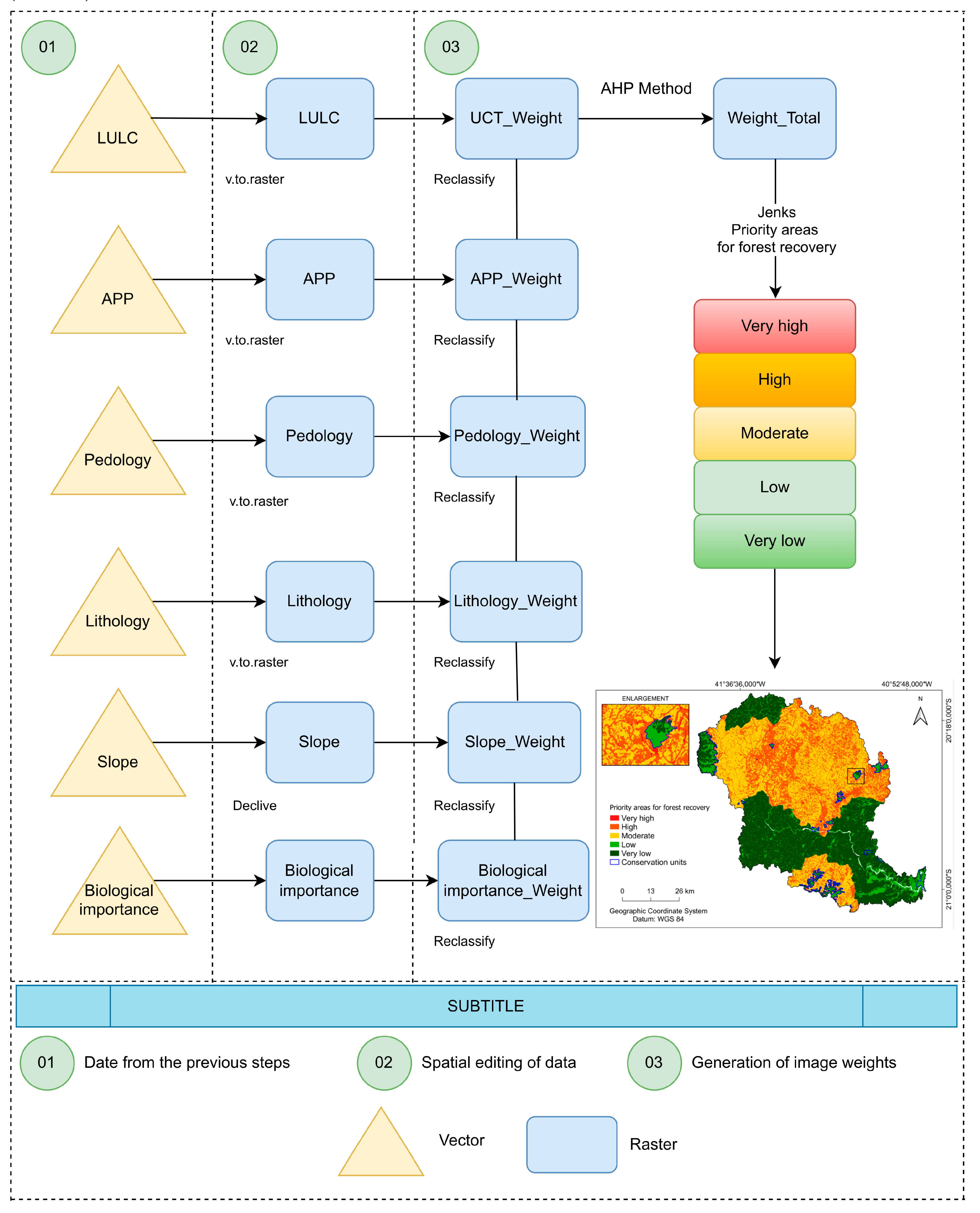
To define the priority areas for recovery and conservation at the BHRI, pedology and lithology data provided by GEOBASES and the thematic map of biological importance available by the Ministry of the Environment - MMA were used. were converted to matrix format (raster), and their respective statistical weight was calculated using the Analytic Hierarchy Process – AHP [36]. Weights from 1 to 100 were assigned to the degree of relevance that the Information Plans (IP) had regarding the conservation of forest fragments and water resources within the hydrographic basin and the ecological corridor, where the lowest values were considered as areas with greater interest for preservation and the highest value, the places with less interest for environmental conservation. In Figure 5 it is possible to visualize the flowchart containing the methodological steps used to delimit the priority areas for forest recovery. The weights for each IP were also defined, according to [37] (Frame 5).

The slope map was made from the Slope tool, using the DEM of the Itapemirim river basin, where it was subsequently reclassified into their respective classes.

With the assigned weights, cost matrix images were generated for each Information Plan (PI). For each raster image, its respective statistical weight was calculated using the Analytic Hierarchy Process – AHP [36]. The AHP is a multicriteria decision method for judging the relative weights of the different factors in the model. Pairwise comparison matrices are constructed and preferences summarized in terms of relative importance value [38] (Table 8).

With the cost matrix images of each parameter and their respective statistical weights, the total cost matrix image was obtained (Equation 16).

{WT}_{2} = P_{1} L U L C_{w} + P_{2} A P P_{w} + P_{3} P E D_{C} + P_{4} L i t_{C} + P_{5} S l o p e_{C} + P_{6} B i o I m p_{W}

(16)

In which,

CT: total cost raster image (dimensionless);

P_{1}

: statistical weight of land use and cover cost raster image (dimensionless);

P_{2}

: statistical weight of APP cost raster image (dimensionless);

P_{3}

: statistical weight of pedology cost raster image (dimensionless);

P_{4}

: statistical weight of lithology cost raster image (dimensionless);

P_{5}

: statistical weight of slope cost raster image (dimensionless);

P_{6}

: statistical weight of biological importance cost raster image (dimensionless);

L U L C_{w}

: land use and cover cost raster image (dimensionless);

A P P_{w}

: APP cost raster image (dimensionless);

P E D_{C}

: pedology cost raster image (dimensionless);

L i t_{C}

: lithology cost raster image (dimensionless);

S l o p e_{C}

: slope cost raster image (dimensionless);

B i o I m p_{W}

: biological importance cost raster image (dimensionless).

2.8. Confrontation of land use and land cover with priority areas for recovery within the EC

The thematic maps of land use and land cover and priority areas were compared using the tool cut to analyze the moderate, high and very high classes, in QGIS version 3.26, since these classes require greater planning and implementation of appropriate conservation measures than the low and very low priority classes.

2.8.1. Costs to define the EC

The values of bare land (VBL) per hectare were based on data from the Federal Revenue for the year 2022. Five classes of land use were considered, as shown in Table 9.

3. Results

The mapping of land use and land cover in the Itapemirim river basin for the year 2021 is shown in Figure 6. The quantification in hectares and the percentages in relation to the study area are shown in Table 10.

3.1. Classification of land use and land cover (LULC)

The predominant use of the basin is Forest, with 27.78% (168,601.94 ha) of the study area. The Forest class occupies 28.35% of the territory (168,601.936 hectares), formed mostly by hilltops, since they make it difficult to use agricultural machinery and implements, and Conservation Units.

3.2. Permanent Preservation Areas (APP)

The mapping of APP in the Itapemirim river basin is shown in Figure 7, and the areas of different types of APP and their respective percentages are shown in Table 11.

The areas close to the springs are of great importance for the supply of water to the watercourses. This APP category is the one that occupies the least area within the BHRI, being associated with the number of mapped springs (576).

Watercourse APPs guarantee the stability of the banks, control soil erosion and water quality, preventing the carry-over of sediments, nutrients and chemicals from the higher parts of the land. This category of APP has its width associated with the width of the water course, since the BHRI has water courses with a width greater than 10 meters. The APP area of watercourses were the ones that showed the greatest expression, constituting 89.88% of the APP area (92,772.71 hectares), equivalent to 15.6% of the basin’s territory.

The slope APPs were obtained through areas with a slope greater than 45º, which is equivalent to 1.332% of the basin area. Due to the topography of the basin, the hilltop APPs have the second lowest expression (2,070.247 hectares), equivalent to 0.35% of the basin’s territory.

3.3. Confrontation of LULC with APP

The results of the confrontation obtained through the tabular crossing of the APP and LULC maps are shown in Figure 8 and Table 12.

The total areas destined for APP, according to the forest code, 68.95% (72,006.311 hectares) are in conflicting use of LULC, while the classes of Forest, Non-Forest Natural Formation, Rocky Outcrops and Water are in accordance with the conserved LULC.

A large part of the APP is degraded due to the negative impact of the Mosaic classes of uses, Agriculture and Pasture (intermediate), since together they occupy 46.61% of the area destined for environmental protection.

The LULC in permanent preservation areas demonstrates the low degree of preservation in which the BHRI finds itself. Due to the low percentage of Forest in the APP (24.04%), in which one of its primary roles cannot be performed, such as soil stability, hydrological control, soil erosion control, avoiding the entrainment of sediments, nutrients and products chemicals.

3.4. Analysis of landscape ecology indices and selection of potential forest fragments using Fuzzy logic

The distribution of forest fragments in the BHRI, by size class, can be seen in Figure 8 and Table 13. 22,007 forest fragments were registered, with a total area of 168,601.936 ha, representing 28.35% of the BHRI area.

The amount of forest fragments present in the BHRI reveals the state of conservation in which the region is faced, in which the importance of diagnoses and practices that promote the conservation of the local flora species stands out.

The largest forest fragments of class C4 present in the BHRI are located in the Conservation Units (UC), namely Caparaó National Park, White Eagle Private Natural Heritage Reserve and Serra das Torres State Natural Monument. This demonstrates the relevance of the conservation units in environmental preservation. It is also noted that the classes of forest fragments C1 and C2 are homogeneously distributed throughout BHRI. In which it does not occur in the same way with forest fragments of larger size, classes C3 and C4, since they form more isolated groupings and with greater distances between fragments of the same class. The BHRI landscape ecology indices are presented in Table 14 by class size.

The edge metrics show the highest total edge value (TE) for the very small fragments class (10,787,900 meters), which is associated with the highest value for the C1 class. Because it is an absolute measure of the total edge length, the study of size classes for this metric may not be relevant for edge density.

Edge density (ED) expresses the value of edge size (TE) in relation to the area occupied by each size class (CA). It is inversely proportional to the area occupied by the size class. Class C4, which has the largest fragment area (100,907.0 ha), has the second highest border density (61.53 m.ha-¹). However, classes C2 and C3 have the lowest edge densities, 31.24 and 11.96 m.ha-¹, respectively.

The mean fractal dimension (MPFD) is the most common shape metric, of which the values of this variable are normally between 1 and 2, and the closer to 1, the simpler the shape of the fragment. Therefore, the greater the fractal dimension and the greater the shape index, the more irregular the fragments. This fact corroborates the results obtained in this study, since fragments from class C4 have the highest value for the fractal dimension, MPFD (1.44) and the highest MSI (6.25), while fragments from class C1 have the lowest values of MSI (1.43), and class C2 fragments had lower MPFD values (1.35). This reinforces that the fragments of class C4 are the ones with the most irregular shapes and those of classes C1 and C2 have more regular shapes. When analyzing the total central area (TCA) of each class, it was observed that class C4 had the highest value, with 73,942.94 ha and class C1 had the lowest TCA, with 4,851.81 ha, determining a smaller edge effect into larger fragments, even though they have a more complex shape.

The degree of isolation of the forest fragments, expressed by the average distance from the nearest neighbor (MNND), showed a direct correlation with the size of the fragment. Fragments of class C4 showed greater isolation (1,785.95 meters) than fragments of class C1 (215.55 meters), which strengthens the importance of fragments of class C1, as elements of connection and biological function, since they can function as ecological corridors and/or trampolines.

The Fuzzy Large function for the variables CA, TCA and TE, where higher values express greater conservation, consequently, greater potential for implementing the ecological corridor, as shown in Figure 10. The Fuzzy Small function allowed representing the gradual variation around the matrix image , in which lower input values are more likely to assume a value of 1, as evidenced in the ED and MSI variables (Figure 11).

The reclassified forest fragments generated from the matrix resulting from the overlapping of selected Landscape Ecology Index (IEP) variables are shown in Figure 12.

The fragments with the highest potential for ecological corridor implementation are present in the Conservation Units (UC) (Figure 11), including Caparaó National Park, Alto da Serra Private Natural Heritage Reserve, Forest of flowers State Park, Forno Grande State Park, Águia Branca Private Natural Heritage Reserve, Fazenda Boa Esperança Private Natural Heritage Reserve, Pacotuba National Forest, and Serra das Torres State Natural Monument.

The majority of the fragments belonging to BHRI were categorized as having low potential for ecological corridor implementation, totaling 18,162 (75.92%) forest fragments in this category.

3.5. Ecological corridor (CE)

The proposal for implementing the corridor to connect the forest fragments of BHRI is presented in Figure 13.

The least-cost path methodology, considering the raster images of UCT, slope, APP, SBCL, and LEI (Fuzzy Gamma), projected the path with the lowest resistance cost along the surface. Two ecological corridors were generated, one between Caparaó National Park and Cachoeira da Fumaça State Park, with a length of 21.27 km and a width of 1064 m, and a second corridor between Cachoeira da Fumaça State Park and Serra das Torres State Natural Monument, spanning 65.96 km in length and 3298 m in width.

The mapping of LULC in the CE of BHRI is presented in Figure 14. The quantification in hectares and the percentages relative to the total area of the CE are presented in Table 15.

The predominant LULC within the ecological corridor is the intermediate pasture class, representing 29.23% of the area (4,284.43 ha). The Forest class has 661 forest fragments within the ecological corridor, but it represents only 22.41% (3,284.19 ha) of the CE area. Over 70% of the territory designated for the ecological corridor is composed of LULC conflicting with the Forest Code, while just over 25% of the same territory is composed of LULC not conflicting with the Forest Code.

3.6. Analysis of priority areas for forest recovery

The mapping of priority areas for forest restoration in BHRI is presented in Figure 15. The quantification in hectares and the percentages relative to the study areas are presented in Table 16.

The criterion that received the highest weight from the application of the AHP method for defining priority areas for forest restoration in BHRI was the Permanent Preservation Areas (APP).

Slope was the fourth factor with the highest weight. Areas with steeper slopes result in increased water velocity and transport capacity, leading to higher susceptibility to erosion in BHRI. When combined with soil type, this vulnerability can be further exacerbated, as soil physical and chemical characteristics also influence erosion.

It is noticeable that a large portion of the areas designated as Conservation Units (UC) remain at Low and Very Low priority levels for restoration and conservation, as they are designated for the preservation of natural ecosystems, preservation of biota, and private areas with predominantly native vegetation cover.

The priority areas map indicated that 57.03% of the area was classified as Very High or High importance, and Moderate priority for forest restoration, while 42.97% (252,932.5 hectares) were considered as Low and Very Low priority for forest restoration.

3.7. Confrontation of LULC with priority areas for recovery within the EC

The results of the tabular cross-matching of the APP and UCT maps are presented in Table 17.

The predominant LULC in relation to the priority areas for restoration within the ecological corridor is the Forest class, followed by Preserved Pasture and Intermediate Pasture, comprising 1,235.75 ha, 1,175.10 ha, and 1,082.26 ha respectively. Non-conflicting classes with the Forest Code cover 1,260.40 ha, while conflicting classes encompass 3,729.74 ha.

3.7.1. Calculation of the Value of Bare Land (VBL) for delimitation of the CE

Based on Table 17, which contains the areas in hectares of land use and land cover (LULC) in relation to the priority areas for restoration within the proposed ecological corridor, and using the VBL values from Table 9, the total VBL was calculated for the delimitation of the proposed ecological corridor, as shown in Table 18.

The LULC with the highest total VBL is Pasture (conserved), followed by Pastagem (intermediary) and Mosaico de usos, where the sum of individual VBL among the classes of Moderate, High, and Very high corresponds to 15,172,747.87 reais, 13,974,071.63 reais, and 13,728,003.44 reais, respectively.

The total VBL per hectare of non-conflicting LULC classes in relation to the priority area for restoration considered "High" presents the highest VBL (3,868,057.47 reais), due to its larger extent (1,007.17 ha), as per Table 17, and the second highest total bare land value per hectare among conflicting LULC classes (21,977,965.57 reais), which reflects in the total VBL for the "High" priority class (25,846,023.04 reais).

The total VBL per hectare of non-conflicting LULC classes in relation to the priority area for restoration considered "Moderate" presents the lowest value of VBL (256,943.65 reais), due to its smaller extent (66.90 ha) as per Table 17, however, it has the highest total VBL per hectare among conflicting LULC classes (25,568,388.49 reais), which contributed to being the second highest total VBL (25,825,332.14 reais).

The total sum of VBL for the priority areas for restoration in the "Moderate," "High," and "Very High" classes corresponds to 52,727,575.02 reais.

4. Discussion

The Atlantic Forest is one of the most threatened regions in the world in terms of biodiversity, with much of its original forest cover already degraded or deforested. Only 12.4% remains as mature and well-preserved forests. It is necessary to monitor and restore the forest, as well as strengthen the legislation that protects it [39]. However, BHRI has 27.4% of its area covered by forest, which shows a higher degree of conservation.

Forests offer a wide range of habitats and resources for the species that inhabit them. Trees provide food, shelter, and breeding sites for many animals, such as birds, primates, felines, and insects [40,41]. The dense vegetation cover also helps to keep the soil moist, retains rainfall, and regulates local temperature, creating microclimates that are ideal for many plant and animal species [40,42].

The spatial distribution of forest fragments in BHRI aligns with the findings of [35], showing that the largest number of fragments (NP) belongs to the class of fragments with sizes smaller than 10 hectares. The moderate-sized fragments (C3) have the lowest values of CA and NP, meaning a smaller area of contact with the surrounding matrix (Table 14). The region surrounding the study area is immersed in a landscape dominated by different pasture classes [43], which enhances the edge effect. According to [44], the composition of the surrounding matrix should be considered when prioritizing measures to increase the area, such as reforestation or isolation of the area, for fragments smaller than 10 hectares.

The high number of C1 class fragments represents a threat to biodiversity conservation and the maintenance of ecosystem processes and services due to the effects of fragmentation. This is a result of the increase in forest edge and the decrease in habitat heterogeneity, which leads to the loss of the central area of these remnants [45,46,47,48]. Due to habitat fragmentation, populations of animals with lower mobility, such as arboreal primates, are most affected, as they depend on tree cover to move [49,50]. As a result, tropical landscapes are becoming a heterogeneous mosaic, and small forest fragments contribute to the simplification of animal communities and partial isolation of wildlife [51]. However, smaller fragments play important roles in the landscape [52], as they can serve as ecological links and stepping stones between large areas, as well as refuges for species [53]

The low predisposition of forest fragments in BHRI was mainly influenced by the metrics CA, TE, and TCA, as they are correlated with landscape ecology analysis. Therefore, it is possible to deduce that the Fuzzy concept can be applied in selecting potential forest fragments for the implementation of ecological corridors [35].

The scenario found in the proposed CE was dominated by the intermediate pasture class, which does not differ much from the historical process that occurred in different regions of the Atlantic Forest, which suffered from poor management of LULC and increased forest fragmentation [54], making it necessary to adopt land use management measures that facilitate the functioning of the corridor.

The maintenance and restoration of corridors are strategies that improve the ability of fauna to survive in small patches of tropical landscapes, which have already suffered from the deforestation process, such as the scenario of the Atlantic Forest [55]. Thus, a new conservation model is necessary for this basin, with a regional-level planning approach, as well as environmental protection or restoration [56].

The results presented for land use and land cover conflicts in APP show that the majority of conflicts were due to improper land use, indicating non-compliance with current environmental legislation (the Forest Code). These results are supported by other studies that analyze conflict zones in APP in the region [57,58]. The New Forest Code, Brazilian environmental legislation, establishes the obligation of landowners to maintain a proportion of forest on their properties, often requiring the restoration of degraded habitats. An additional option for the recovery of degraded pastures is the planting of agroforestry systems (AFS), which combine native species with exotic or fruit species, in compliance with the law [33,59]. The restoration of APP should be carried out through the natural regeneration of native species or the planting of native species, which can be interspersed with exotic species [33]. In addition, other preventive measures should be implemented, such as more effective monitoring by environmental agencies and public management policies focused on the recovery and preservation of these areas, especially APP.

In this study, LCP modeling was used to propose corridors based on land use and land cover classes, slope, APP, landscape ecology index, and subnormal clusters. The methodology allowed assigning greater importance to variables of higher priority for corridor passages. In practice, this is highly relevant for researchers, land managers, and landowners. One disadvantage is that it assumes that animals have a complete knowledge of the landscape and seek to move for specific purposes, however, animals may have their preferred habitat areas and choose travel routes based on other preferences, which may limit the effectiveness of the approach.

The value of land is related to the income that can be obtained from it [60], which explains the higher VBL for the Mosaic class of land use, since it is composed of temporary crops (soybeans, sugar cane, rice, cotton) and perennial crops (coffee and citrus), whether analyzed in terms of monetary productivity or agricultural production [61].

When analyzing the value of bare land for priority areas for restoration in relation to the LULC classes (Table 18), it is noted that the highest investment would be within the priority area for restoration class considered High (25,846,023.04 Brazilian reais), followed by the Moderate class (25,825,332.14 Brazilian reais). The creation of new conservation units in strategic areas within the study area can be effective in increasing landscape connectivity and permeability, favoring the movement of animals and consequently the conservation of biodiversity [62]. In addition, promoting ecological restoration actions in degraded areas can also contribute to improving landscape connectivity and the recovery of populations of species that depend on connectivity for their survival and reproduction, thereby reducing the investment for creating new ecological corridors.

For the conservation of this basin, it is necessary to adopt new concepts for the formation of ecological corridors that address political, social, and environmental aspects in regional-level planning, as well as the protection of landscapes linked to original or restored vegetation [56].

5. Conclusions

The landscape under analysis is mostly covered by forests, indicating a high degree of conservation of the Itapemirim river basin.

The dominant land use and land cover class is reflected in the permanent preservation areas, while in the proposed ecological corridor, the predominant class is pasture (intermediar), which has the majority of its areas in conflict with current legislation.

The forest fragments in the Itapemirim river basin are mostly represented by fragments smaller than 10 hectares.

The technique of associating landscape ecology indices through Fuzzy logic has proven to be an alternative for selecting potential fragments for determining ecological corridors.

The least-cost path algorithm correlated with the results generated by the multicriteria decision-making method (AHP) represents an important tool for planning and implementing ecological corridors.

The LULC class with the highest VBL per hectare within the ecological corridor is Pasture (conserved), followed by Pasture (intermediary) and Mosaic of uses, as they have the highest total VBL among all other LULC classes, due to the income that can be obtained from them.

The mapping of priority areas for forest restoration in the Itapemirim river watershed using specialized numerical levels optimizes the implementation of native forest cover restoration projects. The priority for forest restoration showed a significant intersection with the areas associated with permanent preservation areas (APP).

The proposed methodology for implementing ecological corridors and mapping priority areas for forest restoration can be applied to other basin, phytophysiognomies, and biomes.

Author Contributions

Conceptualization, V.D.N.M, H.M.D, T.R.M, R.C.F.C. and A.R.S.; methodology, V.D.N.M, H.M.D. T.R.M. and A.R.S.; validation, V.D.N.M., H.M.D, T.R.M, R.C.F.C and A.R.S.; formal analysis, H.M.D, A.R.S, T.R.M, R.C.F.C, E.C.S, C.P and C.U.Z.; investigation, V.D.N.M.and A.R.S.; resources, V.D.N.M; data curation, V.D.N.M, H.M.D, A.R.S, T.R.M, R.C.F.C, E.C.S, C.P and C.U.Z.; writing—original draft preparation, H.M.D, A.R.S, T.R.M, R.C.F.C, E.C.S, C.P and C.U.Z.; writing—review and editing, V.D.N.M.. and R.C.F.C.; supervision, H.M.D. and A.R.S; project administration, V.D.N.M, H.M.D and A.R.S.; funding acquisition, V.D.N.M.and H.M.D. All authors have read and agreed to the published version of the manuscript.

Funding

This research received no external funding.

Institutional Review Board Statement

Not applicable.

Informed Consent Statement

Not applicable.

Data Availability Statement

No new data were created or analyzed in this study. Data sharing is not applicable to this article.

Acknowledgments

The authors thank the following bodies for making the database available for the development of the research: The Coordination for the Improvement of Higher Education Personnel (CAPES). Finally, the authors would like to thank the Graduate Program in Forest Sciences at the Federal University of Espírito Santo and the research group Geotechnology Applied to the Global Environment (GAGEN), registered with CNPq.

Conflicts of Interest

The authors declare no conflict of interest.

References

Ferreira, P.A.; Boscolo, D.; Viana, B.F. What Do We Know about the Effects of Landscape Changes on Plant–Pollinator Interaction Networks? Ecol. Indic. 2013, 31, 35–40. [Google Scholar] [CrossRef]
Agência Estadual de Recursos Hídricos - AGERH Comitês de Bacias Hidrográficas. Available online: https://agerh.es.gov.br (accessed on 29 November 2021).
Frechiani, J.M.; Marchioro, E. Transformação No Uso e Cobertura Da Terra Associado a Mineração No Distrito de Itaoca, Cachoeiro de Itapemirim (ES). Rev. Geogr. 2012. [Google Scholar]
Pirovani, D.B.; da Silva, A.G.; dos Santos, A.R.; Cecílio, R.A.; Gleriani, J.M.; Martins, S.V.; da Silva, A.G.; dos Santos, A.R.; Cecílio, R.A.; Gleriani, J.M.; et al. Análise Espacial de Fragmentos Florestais Na Bacia Do Rio Itapemirim, ES. Rev. Árvore 2014, 38, 271–281. [Google Scholar] [CrossRef]
Fahrig, L. Effects of Habitat Fragmentation on Biodiversity. Annu. Rev. Ecol. Evol. Syst. 2003, 34, 487–515. [Google Scholar] [CrossRef]
Dias, P.; Gomes, L.; Callegaro, R.; Carvalho, F.; Dias, H. STRUCTURAL AND ENVIRONMENTAL VARIABILITY FROM THE EDGE TO THE INTERIOR OF AN ATLANTIC FOREST REMNANT IN BRAZIL. J. Trop. For. Sci. 2021, 33, 308–332. [Google Scholar] [CrossRef]
Magnago, L.F.S.; Edwards, D.P.; Edwards, F.A.; Magrach, A.; Martins, S. V.; Laurance, W.F. Functional Attributes Change but Functional Richness Is Unchanged after Fragmentation of Brazilian Atlantic Forests. J. Ecol. 2014, 102, 475–485. [Google Scholar] [CrossRef]
Pereira Gomes, L.; Borges Dias, P.; Machado Dias, H.; Horn Kunz, S. Growing at the Forest Edges: How Natural Regeneration Develops under Fragmentation. iForest - Biogeosciences For. 2022, 15, 248–255. [Google Scholar] [CrossRef]
Guimarães, H.; Braga, R.; Mascarenhas, A.; Ramos, T.B. Indicators of Ecosystem Services in a Military Atlantic Forest Area, Pernambuco—Brazil. Ecol. Indic. 2017, 80, 247–257. [Google Scholar] [CrossRef]
Taffarello, D.; Calijuri, M. do C.; Viani, R.A.G.; Marengo, J.A.; Mendiondo, E.M. Hydrological Services in the Atlantic Forest, Brazil: An Ecosystem-Based Adaptation Using Ecohydrological Monitoring. Clim. Serv. 2017, 8, 1–16. [Google Scholar] [CrossRef]
Tabarelli, M.; Aguiar, A.V.; Ribeiro, M.C.; Metzger, J.P.; Peres, C.A. Prospects for Biodiversity Conservation in the Atlantic Forest: Lessons from Aging Human-Modified Landscapes. Biol. Conserv. 2010, 143, 2328–2340. [Google Scholar] [CrossRef]
Gross, M. Brazil’s Fragmented Forests. Curr. Biol. 2017, 27, R681–R684. [Google Scholar] [CrossRef]
Ferrari, J.L.; Silva, S.F.; Santos, A.R.; Garcia, R.F. Corredores Ecológicos Potenciais Na Sub-Bacia Hidrográfica Do Córrego Horizonte, Alegre-ES, Indicados Por Meio de SIG. Rev. Bras. Ciências Agrárias - Brazilian J. Agric. Sci. 2012, 7, 133–141. [Google Scholar] [CrossRef]
Louzada Franciane, L.R. de O.; Dos Santos, A.R.; da Silva, A.G.; de Oliveira, O.M.; de Oliveira, G.G.; Paulo, S.V.; Batista Esteves, P.J. Proposta de Corredores Ecológicos Para Interligação de Parques Estaduais Utilizando Geotecnologia, Espirito Santo (ES)-Brasil. Rev. Geogr. Venez. 2013, 53, 239–254. [Google Scholar]
Dondina, O.; Kataoka, L.; Orioli, V.; Bani, L. How to Manage Hedgerows as Effective Ecological Corridors for Mammals: A Two-Species Approach. Agric. Ecosyst. Environ. 2016, 231, 283–290. [Google Scholar] [CrossRef]
Hofman, M.P.G.; Hayward, M.W.; Kelly, M.J.; Balkenhol, N. Enhancing Conservation Network Design with Graph-Theory and a Measure of Protected Area Effectiveness: Refining Wildlife Corridors in Belize, Central America. Landsc. Urban Plan. 2018, 178, 51–59. [Google Scholar] [CrossRef]
Hong, W.; Guo, R.; Su, M.; Tang, H.; Chen, L.; Hu, W. Sensitivity Evaluation and Land-Use Control of Urban Ecological Corridors: A Case Study of Shenzhen, China. Land use policy 2017, 62, 316–325. [Google Scholar] [CrossRef]
Liang, J.; He, X.; Zeng, G.; Zhong, M.; Gao, X.; Li, X.; Li, X.; Wu, H.; Feng, C.; Xing, W.; et al. Integrating Priority Areas and Ecological Corridors into National Network for Conservation Planning in China. Sci. Total Environ. 2018, 626, 22–29. [Google Scholar] [CrossRef]
ROCHA, M.A.M. Manejo de Plantas Daninhas. In Café Conilon; INCAPER: Vitória, ES, 2007; pp. 391–404. [Google Scholar]
Recio, M.R.; Seddon, P.J.; Moore, A.B. Niche and Movement Models Identify Corridors of Introduced Feral Cats Infringing Ecologically Sensitive Areas in New Zealand. Biol. Conserv. 2015, 192, 48–56. [Google Scholar] [CrossRef]
Ribeiro, M.P.; de Mello, K.; Valente, R.A. How Can Forest Fragments Support Protected Areas Connectivity in an Urban Landscape in Brazil? Urban For. Urban Green. 2022, 74, 127683. [Google Scholar] [CrossRef]
Peng, J.; Yang, Y.; Liu, Y.; Hu, Y.; Du, Y.; Meersmans, J.; Qiu, S. Linking Ecosystem Services and Circuit Theory to Identify Ecological Security Patterns. Sci. Total Environ. 2018, 644, 781–790. [Google Scholar] [CrossRef]
Santos, J.S.; Leite, C.C.C.; Viana, J.C.C.; dos Santos, A.R.; Fernandes, M.M.; de Souza Abreu, V.; do Nascimento, T.P.; dos Santos, L.S.; de Moura Fernandes, M.R.; da Silva, G.F.; et al. Delimitation of Ecological Corridors in the Brazilian Atlantic Forest. Ecol. Indic. 2018, 88, 414–424. [Google Scholar] [CrossRef]
Perkl, R.M. Geodesigning Landscape Linkages: Coupling GIS with Wildlife Corridor Design in Conservation Planning. Landsc. Urban Plan. 2016, 156, 44–58. [Google Scholar] [CrossRef]
Strnad, D.; Kohek, Š.; Kolmanič, S. Fuzzy Modelling of Growth Potential in Forest Development Simulation. Ecol. Inform. 2018, 48, 80–88. [Google Scholar] [CrossRef]
Teixeira, T.R.; Soares Ribeiro, C.A.A.; Rosa dos Santos, A.; Marcatti, G.E.; Lorenzon, A.S.; de Castro, N.L.M.; Domingues, G.F.; Leite, H.G.; da Costa de Menezes, S.J.M.; Santos Mota, P.H.; et al. Forest Biomass Power Plant Installation Scenarios. Biomass and Bioenergy 2018, 108, 35–47. [Google Scholar] [CrossRef]
Biazatti, L.D.; Fiedler, N.C.; Ramalho, A.H.C.; Moreira, T.R.; Rezende, G.F. MAPPING THE RISK OF FOREST FIRES IN THE RIO PRETO NATIONAL FOREST IN THE ATLANTIC FOREST. FLORESTA 2021, 51, 1062. [Google Scholar] [CrossRef]
Ramalho, A.H.C.; Santos, A.R. dos; Fiedler, N.C.; Biazatti, L.D.; Menezes, R.A.S.; Lucas, F.M.F.; Aragão, M. Aragão, M. de A.; Júnior, A.O.N. Zoneamento de Risco de Ocorrência de Incêndios Florestais - Passo a Passo; Antônio Henrique, 2021; ISBN 9786500322040.
Agência Estadual de Recursos Hídricos - AGERH Manual Operativo Dos Planos de Recursos Hídricos Capixabas: Bacia Hidrográfica Do Rio Itapemirim: De Olho No Rio: Do Plano Ao MOP; Espírito Santo, 2020.
Senhorelo, A.P.; Sousa, E.F. de; Santos, A.R. dos; Ferrari, J.L.; Peluzio, J.B.E.; Zanetti, S.S.; Carvalho, R. de C.F.; Camargo Filho, C.B.; Souza, K.B. de; Moreira, T.R.; et al. Application of the Vegetation Condition Index in the Diagnosis of Spatiotemporal Distribution of Agricultural Droughts: A Case Study Concerning the State of Espírito Santo, Southeastern Brazil. Diversity 2023, 15, 460. [Google Scholar] [CrossRef]
Anderson, L.O.; Ribeiro Neto, G.; Cunha, A.P.; Fonseca, M.G.; Mendes de Moura, Y.; Dalagnol, R.; Wagner, F.H.; de Aragão, L.E.O. e C. Vulnerability of Amazonian Forests to Repeated Droughts. Philos. Trans. R. Soc. B Biol. Sci. 2018, 373, 20170411. [Google Scholar] [CrossRef]
MapBiomas MapBiomas Collection - Coleção 6 Available online:. Available online: https://mapbiomas.org (accessed on 26 November 2021).
BRASIL Novo Código Florestal Brasileiro, Lei N^o 12.651, de 25 de Maio de 2012; 2012.
Jiang, H.; Eastman, J.R. Application of Fuzzy Measures in Multi-Criteria Evaluation in GIS. Int. J. Geogr. Inf. Sci. 2000, 14, 173–184. [Google Scholar] [CrossRef]
Moreira, T.R. Proposta de Implantação de Corredores Ecológicos Como Estratégia Para Mitigação de Impactos Ambientais Na Bacia Hidrográfica Do Rio Doce, Brasil, Universidade Federal do Espírito Santo, 2019.
Saaty, T.L. A Scaling Method for Priorities in Hierarchical Structures. J. Math. Psychol. 1977, 15, 234–281. [Google Scholar] [CrossRef]
De Almeida, F.C.; Silveira, E.M.D.O.; Acerbí Junior, F.W.; França, L.C.D.J.; Bueno, I.T.; Terra, B.J.O. ANÁLISE MULTICRITÉRIO NA DEFINIÇÃO DE ÁREAS PRIORITÁRIAS PARA RECUPERAÇÃO FLORESTAL NA BACIA DO RIO DOCE, EM MINAS GERAIS. Nativa 2020, 8, 81. [Google Scholar] [CrossRef]
Li, H.; Li, D.; Li, T.; Qiao, Q.; Yang, J.; Zhang, H. Application of Least-Cost Path Model to Identify a Giant Panda Dispersal Corridor Network after the Wenchuan Earthquake—Case Study of Wolong Nature Reserve in China. Ecol. Modell. 2010, 221, 944–952. [Google Scholar] [CrossRef]
SOSMA - Fundação, S.O. S Mata Atlântica Relatório Anual 2021. Relatório Anu. 2021 2021, 1, 80. [Google Scholar]
Goatley, C.H.R.; Bellwood, D.R. The Roles of Dimensionality, Canopies and Complexity in Ecosystem Monitoring. PLoS One 2011, 6, e27307. [Google Scholar] [CrossRef] [PubMed]
Gómez-Creutzberg, C.; Lagisz, M.; Nakagawa, S.; Brockerhoff, E.G.; Tylianakis, J.M. Consistent Trade-offs in Ecosystem Services between Land Covers with Different Production Intensities. Biol. Rev. 2021, 96, 1989–2008. [Google Scholar] [CrossRef]
Dale, A.G.; Frank, S.D. Urban Warming Trumps Natural Enemy Regulation of Herbivorous Pests. Ecol. Appl. 2014, 24, 1596–1607. [Google Scholar] [CrossRef]
Pirovani, D.B.; Silva, A.G. da; Santos, A.R. dos ANÁLISE DA PAISAGEM E MUDANÇAS NO USO DA TERRA NO ENTORNO DA RPPN CAFUNDÓ, ES. CERNE 2015, 21, 27–35. [Google Scholar] [CrossRef]
Santos, J.S.; Leite, C.C.C.; Viana, J.C.C.; dos Santos, A.R.; Fernandes, M.M.; de Souza Abreu, V.; do Nascimento, T.P.; dos Santos, L.S.; de Moura Fernandes, M.R.; da Silva, G.F.; et al. Delimitation of Ecological Corridors in the Brazilian Atlantic Forest. Ecol. Indic. 2018, 88, 414–424. [Google Scholar] [CrossRef]
Haddad, N.M.; Brudvig, L.A.; Clobert, J.; Davies, K.F.; Gonzalez, A.; Holt, R.D.; Lovejoy, T.E.; Sexton, J.O.; Austin, M.P.; Collins, C.D.; et al. Habitat Fragmentation and Its Lasting Impact on Earth’s Ecosystems. Sci. Adv. 2015, 1. [Google Scholar] [CrossRef]
Moraes, M.C.P. de; Mello, K. de; Toppa, R.H. ANÁLISE DA PAISAGEM DE UMA ZONA DE AMORTECIMENTO COMO SUBSÍDIO PARA O PLANEJAMENTO E GESTÃO DE UNIDADES DE CONSERVAÇÃO. Rev. Árvore 2015, 39, 1–8. [Google Scholar] [CrossRef]
Pfeifer, M.; Lefebvre, V.; Peres, C.A.; Banks-Leite, C.; Wearn, O.R.; Marsh, C.J.; Butchart, S.H.M.; Arroyo-Rodríguez, V.; Barlow, J.; Cerezo, A.; et al. Creation of Forest Edges Has a Global Impact on Forest Vertebrates. Nature 2017, 551, 187–191. [Google Scholar] [CrossRef]
Silva, V.L.; Mehltreter, K.; Schmitt, J.L. Ferns as Potential Ecological Indicators of Edge Effects in Two Types of Mexican Forests. Ecol. Indic. 2018, 93, 669–676. [Google Scholar] [CrossRef]
Estrada, A.; Garber, P.A.; Rylands, A.B.; Roos, C.; Fernandez-Duque, E.; Di Fiore, A.; Nekaris, K.A.-I.; Nijman, V.; Heymann, E.W.; Lambert, J.E.; et al. Impending Extinction Crisis of the World’s Primates: Why Primates Matter. Sci. Adv. 2017, 3. [Google Scholar] [CrossRef] [PubMed]
Moraes, A.M.; Ruiz-Miranda, C.R.; Galetti Jr., P. M.; Niebuhr, B.B.; Alexandre, B.R.; Muylaert, R.L.; Grativol, A.D.; Ribeiro, J.W.; Ferreira, A.N.; Ribeiro, M.C. Landscape Resistance Influences Effective Dispersal of Endangered Golden Lion Tamarins within the Atlantic Forest. Biol. Conserv. 2018, 224, 178–187. [Google Scholar] [CrossRef]
Ripperger, S.P.; Tschapka, M.; Kalko, E.K.V.; Rodríguez-Herrera, B.; Mayer, F. Resisting Habitat Fragmentation: High Genetic Connectivity among Populations of the Frugivorous Bat Carollia Castanea in an Agricultural Landscape. Agric. Ecosyst. Environ. 2014, 185, 9–15. [Google Scholar] [CrossRef]
Fletcher, R.J.; Didham, R.K.; Banks-Leite, C.; Barlow, J.; Ewers, R.M.; Rosindell, J.; Holt, R.D.; Gonzalez, A.; Pardini, R.; Damschen, E.I.; et al. Is Habitat Fragmentation Good for Biodiversity? Biol. Conserv. 2018, 226, 9–15. [Google Scholar] [CrossRef]
Pütz, S.; Groeneveld, J.; Alves, L.F.; Metzger, J.P.; Huth, A. Fragmentation Drives Tropical Forest Fragments to Early Successional States: A Modelling Study for Brazilian Atlantic Forests. Ecol. Modell. 2011, 222, 1986–1997. [Google Scholar] [CrossRef]
Ribeiro, M.C.; Metzger, J.P.; Martensen, A.C.; Ponzoni, F.J.; Hirota, M.M. The Brazilian Atlantic Forest: How Much Is Left, and How Is the Remaining Forest Distributed? Implications for Conservation. Biol. Conserv. 2009, 142, 1141–1153. [Google Scholar] [CrossRef]
Pardini, R.; Bueno, A. de A.; Gardner, T.A.; Prado, P.I.; Metzger, J.P. Beyond the Fragmentation Threshold Hypothesis: Regime Shifts in Biodiversity Across Fragmented Landscapes. PLoS One 2010, 5, e13666. [Google Scholar] [CrossRef]
da Silva, J.M.C.; Tabarelli, M. Tree Species Impoverishment and the Future Flora of the Atlantic Forest of Northeast Brazil. Nature 2000, 404, 72–74. [Google Scholar] [CrossRef]
Luppi, A.S.L.; dos Santos, A.R.; Eugenio, F.C.; Feitosa, L.S.A.; Luppi, A.S.L.; Rosa dos Santos, A.; Eugenio, F.C.; Feitosa, L.S.A. Utilization of Geotechnology for the Mapping of Permanent Preservation Areas in João Neiva, Espirito Santo State, Brazil. Floresta e Ambient. 2015, 22, 13–22. [Google Scholar] [CrossRef]
Moreira, T.R.; Santos, A.R. dos; Dalfi, R.L.; Campos, R.F. de; Santos, G.M.A.D.A. dos; Eugenio, F.C. Confronto Do Uso e Ocupação Da Terra Em APPs No Município de Muqui, ES. Floresta e Ambient. 2015, 22, 141–152. [Google Scholar] [CrossRef]
Brasil Lei Federal N° 12.854, de 26 de Agosto de 2013; Brasil, 2013.
Ferro, A.B.; Castro, E.R. de Determinantes Dos Preços de Terras No Brasil: Uma Análise de Região de Fronteira Agrícola e Áreas Tradicionais. Rev. Econ. e Sociol. Rural 2013, 51, 591–609. [Google Scholar] [CrossRef]
Marques, F.C.; Telles, T.S. Os Efeitos Espaciais São Fatores Determinantes Dos Preços Das Terras Agrícolas No Brasil. Rev. Econ. e Sociol. Rural 2023, 61. [Google Scholar] [CrossRef]
Pardini, R.; de Souza, S.M.; Braga-Neto, R.; Metzger, J.P. The Role of Forest Structure, Fragment Size and Corridors in Maintaining Small Mammal Abundance and Diversity in an Atlantic Forest Landscape. Biol. Conserv. 2005, 124, 253–266. [Google Scholar] [CrossRef]

Figure 1. Hidrographic basin of the Itapemirim river, with emphasis on forest remnants and protected areas.

Figure 2. Flowchart containing the methodology used for delimitation of APP in the BHRI, according to the legislation.

Figure 3. Metodological flowchart for the characterization of landscape ecology indices and selection of forest fragments in the BHRI.

Figure 4. Methodological flowchart for delimitation of the ecological corridor.

Figure 5. Methodological flowchart for delimitation of priority areas for forest recovery.

Figure 6. Classes of use and land cover of the Itapemirim river basin for the year 2021.

Figure 7. Permanent preservation areas of the Itapemirim river basin, ES, Brazil.

Figure 8. Confrontation of LULC in relation to APP Total.

Figure 9. Forest fragments by size class, in the Itapemirim river basin.

Figure 10. Spatial discretization of the fuzzy variables of CA, TCA and TE at BHRI.

Figure 11. Spatial discretization of the fuzzy variables of ED and MSI in the BHRI.

Figure 12. Classification of potential forest fragments to constitute the ecological corridor at BHRI.

Figure 13. Proposed ecological corridor between Caparaó National Park and Serra das Torres State Natural Monument.

Figure 14. LULC in the proposed CE between Caparaó National Park and Serra das Torres State Natural Monument.

Figure 15. Priority areas for forest restoration in BHRI.

Table 1. Accuracy analysis of land use and land cover.

Year 2021	Porcentage (%)
Overall accuracy	90.99
Area Disagreement	2.33
Allocation disagreement	6.67

Table 3. Costs attributed to permanent preservation areas, with the aim of generating a cost surface to trace the path of the ecological corridor.

Permanent Preservation Areas	Costs
No permanent preservation areas	100
With areas of permanent preservation	1

Table 4. Costs attributed to subnormal agglomerations, with the aim of generating a cost surface to trace the paths of the ecological corridor.

Subnormal clusters (SBCL)	Costs
With subnormal clusters	100
No subnormal clusters	1

Table 5. Costs attributed to forest fragments, with the aim of generating a cost surface to trace the paths of the ecological corridor.

Forest fragments	Costs
No forest fragments	30
Very low potential forest fragments	20
Low potential forest fragments	10
Moderate potential forest fragments	5
High potential forest fragments	2
Very high potential forest fragments	1

Table 6. Costs attributed to the different slope classes, with the aim of generating a cost surface to trace the paths of the ecological corridor.

Slope	Classes	Costs
>45º	High	100
20 – 45º	Moderate	50
<20º	Low	1

Table 7. Paired comparison matrix and the statistical weights obtained by the AHP method for the elaboration of the ecological corridor.

	Slope	APP	LEI	LULC	SBCL	Statistical weights
Slope	1	1/3	1/5	1/9	1/3	0.0453
APP	3	1	1/3	1/5	1	0.1148
LEI	5	3	1	1/3	1	0.2123
LULC	9	5	3	1	1	0.4223
SBCL	3	1	1	1	1	0.2050

Table 8. Paired comparison matrix and the statistical weights obtained by the AHP method for the elaboration of priority areas for recovery and conservation.

	Slope	APP	LULC	Pedology	Lithology	Biological importance	Statistical weight
Slope	1	1/3	1/5	1	1/3	1/5	0.0524
APP	3	1	1/5	1	1	1/3	0.0986
LULC	5	5	1	1	1	1/5	0.1877
Pedology	1	1	1	1	1	1/5	0.0964
Lithology	3	1	1	1	1	1/5	0.1122
Biological importance	5	3	5	5	5	1	0.4523

Table 9. Bare land values assigned to land cover classes.

LULC classes	Bare land values ($)
Mosaic of uses	15,239.52
Pasture	12,911.90
Forest plantation	6,400.88
Preservation of Fauna and Flora	3,840.54
Others	8,511.52

Table 10. Land use and land cover of the Itapemirim river basin for the year 2021.

	Land use and land cover
	Classes	Area (ha)	Porcentage (%)
	Forest	168601.94	27.781
	Non forest natural formation	3846.444	0.634
	Forest plantation	4951.021	0.816
	Rocky outcrop	14054.74	2.316
	Agriculture	51860.467	8.545
	Pasture (conserved)	106947.098	17.622
	Pasture (intermediary)	115902.160	19.098
	Pasture (severely degraded)	21695.150	3.575
	Mosaico f uses	110185.474	18.156
	Urban area	5703.274	0.940
	Wate	2145.61	0.354
	Other non vegetated áreas	982.28	0.162
	Paved and unpaved roads	21.51	0.004
Total		606897.167	100

Table 11. Areas of different types of APP and their percentages in relation to the total APP areas for the basin.

Classes of APP		Area (ha)	Porcentagem (%)	Percentage of Itapemirim river basin (%)
	APP of springs	444.685	0.431	0.075
	APP of water courses	92,772.71	89.889	15.603
	APP of slope	7,919.98	7.674	1.332
	APP of top of hill	2,070.247	2.006	0.348
Total		103,207.626	100	17.358

Table 12. Confrontation of LULC in relation to the total APP.

LULC in the total APP
Classes		Year 2021
Classes		Area (ha)	Porcentage (%)
Non-conflicting		Area (ha)	Porcentage (%)
	Forest	25,104.37	24.04
	Formação natural não florestal	560.74	0.54
	Rockys outcrop	4981.81	4.77
	Water	1786.43	1.71
Total non-conflicting		32433.34	31.05
Conflicting		Area (ha)	Porcentage (%)
	Forest plantation	497.556	0.48
	Agriculture	7,230.84	6.92
	Pasture (conserved)	17,645.60	16.90
	Pasture (intermediary)	17,086.10	16.36
	Pasture (severely degraded)	3,433.81	3.29
	Mosaic of uses	24,367.03	23.33
	Urban área	1,551.71	1.49
	Other non vegetated áreas	193.173	0.18
	Paved and unpaved roads	0.485	0.00
Total conflicting		72,006.311	68.95
Total		104,439.65	100

Table 13. Areas of different sizes of forest fragments and their percentages in relation to the sum of the area of fragment classes.

Fragment size classes		Area (ha)	Porcentage (%)
	C1 – Very small (< 10 ha)	26,403.941	15.67
	C2 - Small (10 - 50 ha)	27,912.638	16.557
	C3 - Moderate (50 - 100 ha)	13,417.911	7.96
	C4 - Large (≥ 100 ha)	100,845.648	59.82
Total		168,580.138	100

Table 14. Landscape ecology indices calculated for the Itapemirim river basin area.

Group	Initials	Unit	Class size (ha)
Group	Initials	Unit	C1(< 10)	C2(10 - 50)	C3(50 - 100)	C4(≥ 100)
Area	CA	ha	26,422.7	27,932.4	13,426.8	100,907.0
Density and Size	NP	Adim.	20.311	1.328	197	171
	MPS	ha	1.80	21.67	68.85	668.25
	PSSD	ha	1.86	10.18	13.36	1,292.83
	PSCoV	%	143.09	48.38	19.61	219.09
Edge	TE	m	10,787,900.0	5,269,320.0	2,017,620.0	10,379,300.0
Edge	ED	m.ha-¹	63.95	31.24	11.96	61.53
Shape	MSI	Adim.	1.43	2.45	3.50	6.25
Shape	MPFD	Adim.	1.36	1.35	1.37	1.44
Central area	TCA	ha	4,851.81	13,860.81	78,88.41	73,942.94
Proximity	MNND	m	215.55	1,061.01	2,693.49	1,785.95

CA (Area of all fragments of the class); NP (Number of fragments); MPS (Average fragment size); PSSD (Standard Deviation of Fragment Size); PSCoV (Coefficient of Variation of Fragment Size); TE (Total edges); ED (Edge Density); MSI (Average Shape Index); MPFD (Average Fractal Dimension); NCA (Total number of central areas); TCA (Total central area); MNND (Average Nearest Neighbor Distance).

Table 15. LULC in the proposed ecological corridor in the Itapemirim river basin.

Classes		Year 2021
Classes		Area (ha)	Porcentage (%)
Non-conflicting		Area (ha)	Porcentage (%)
	Forest	3,284.19	22.41
	Rockys outcrop	170.79	1.17
	Water	245.22	1.67
Total non-conflicting		3,700.20	25.25
Conflicting		Area (ha)	Porcentage (%)
	Forest plantation	89.54	0.61
	Agriculture	458.15	3.13
	Pasture (conserved)	2,780.87	18.97
	Pasture (intermediary)	4,284.43	29.23
	Pasture (severely degraded)	1041.14	7.10
	Mosaic of uses	2,237.85	15.27
	Urban area	60.15	0.41
	Other non vegetated area	4.59	0.03
Total conflicting		10,956.72	74.75
Total		14,656.92	100

Table 16. Priority areas for forest recovery at BHRI.

Jenks		Area (ha)	Porcentage (%)
	Very high	16,817.1	2.86
	High	170,709.0	29.01
	Moderate	148,078.0	25.16
	Low	97,299.5	16.53
	Very low	155,633.0	26.44
Total		588,536.6	100

Table 17. Comparison of LULC with priority areas for restoration within the CE.

LULC		Priority areas for recovery
Non-conflicting		Moderate (ha)	High(ha)	Very High (ha)	(∑)
	Forest	48.557	1000.87	186.33	1235.75
	Rockys outcrop	18.256	3.598	0	21.85
	Water	0.09	2.697	0	2.79
Total non-conflicting		66.90	1.007.17	186.33	1260.40
Conflicting		Moderate (ha)	High (ha)	Very high (ha)	(∑)
	Forest plantation	16.451	4.765	0.09	21.31
	Agriculture	349.177	77.437	14.654	441.27
	Pasture (conserved)	598.976	574.593	1.529	1,175.10
	Pasture (intermediary)	610.964	468.782	2.517	1,082.26
	Pasture (severely degraded)	20.41	23.29	0	43.70
	Mosaic of uses	409.198	480.917	10.701	900.82
	Urban area	42.085	20.321	0	62.41
	Other non vegetated areas	1.169	1.619	0	2.79
	Paved and unpaved roads	0.09	0	0	0.09
Total conflicting		2,048.52	1,651.72	29.49	3,729.74
(∑)		2,115.42	2,658.89	215.82	4,990.13

Table 18. Bare land value per priority areas for restoration in relation to LULC classes.

LULC		Bare land value (VBL) per priority area for restoration
Non-conflicting		Moderate ($)	High ($)	Very high ($)
	Forest	186,485.10	3,843,881.27	715,596.30
	Rockys outcrop	70,112 .90	1,381.26	0
	Water	345.65	10,357.94	0
Total non-conflicting		256,943.65	3,868,057 .47	715,596.30
Conflicting		Moderate ($)	High ($)	Very high ($)
	Forest plantation	105,300.88	30,500.19	576.08
	Agriculture	2,972,027 .02	659,106.57	124,727.81
	Pasture (conserved)	7,733,918.21	7,419,087.36	19,742.30
	Pasture (intermediary)	7,888,706.07	6,052,866.31	32,499.25
	Pasture (severeçy degraded)	263,531.88	300,718.15	0
	Mosaic of uses	6,235,981.10	7,328,944 .24	163,078.10
	Urban area	358,207.32	172,962.60	0
	Other non vegetated areas	9,949.97	13,780.15	0
	Paved and unpaved roads	766.04	0	0
Total conflicting		25,568,388.49	21,977,965.57	340,623.54
Summation		25,825,332.14	25,846,023.04	1,056,219.84

Disclaimer/Publisher’s Note: The statements, opinions and data contained in all publications are solely those of the individual author(s) and contributor(s) and not of MDPI and/or the editor(s). MDPI and/or the editor(s) disclaim responsibility for any injury to people or property resulting from any ideas, methods, instructions or products referred to in the content.

© 2023 by the authors. Licensee MDPI, Basel, Switzerland. This article is an open access article distributed under the terms and conditions of the Creative Commons Attribution (CC BY) license (https://creativecommons.org/licenses/by/4.0/).

Copyright: This open access article is published under a Creative Commons CC BY 4.0 license, which permit the free download, distribution, and reuse, provided that the author and preprint are cited in any reuse.

MDPI Initiatives

Important Links

Choose an area of interest and we will send you notifications of new preprints at your preferred frequency.

Disclaimer

Delimitation of Ecological Corridor Using Technological Tools

Abstract

1. Introduction

2. Materials and Methods

2.1. Characterization of the study area

2.2. Database

2.2.1. Land use land cover (LULC)

2.3. Delimitation of permanent preservation areas (APP)

2.4. Comparison of land use and land cover with permanent preservation areas (APP)

2.5. Selection of forest fragments based on landscape ecology metrics índices

2.5.1. Landscape ecology metrics indices

2.5.2. Selection of forest fragments using Fuzzy logic

2.6. Delimitation of the ecological corridor (EC)

2.7. Priority areas for forest recovery

2.8. Confrontation of land use and land cover with priority areas for recovery within the EC

2.8.1. Costs to define the EC

3. Results

3.1. Classification of land use and land cover (LULC)

3.2. Permanent Preservation Areas (APP)

3.3. Confrontation of LULC with APP

3.4. Analysis of landscape ecology indices and selection of potential forest fragments using Fuzzy logic

3.5. Ecological corridor (CE)

3.6. Analysis of priority areas for forest recovery

3.7. Confrontation of LULC with priority areas for recovery within the EC

3.7.1. Calculation of the Value of Bare Land (VBL) for delimitation of the CE

4. Discussion

5. Conclusions

Author Contributions

Funding

Institutional Review Board Statement

Informed Consent Statement

Data Availability Statement

Acknowledgments

Conflicts of Interest

References

MDPI Initiatives

Important Links

Subscribe