Submitted:
09 April 2023
Posted:
11 April 2023
Read the latest preprint version here
Abstract
The makeup of human microbiota has been linked to a number of autoimmune disorders. Recent developments in whole metagenome sequencing and 16S rRNA sequencing technology have considerably aided research into the microbiome and its relationship to disease. Due to the inherent high dimensionality and complexity of data generated by high-throughput platforms, conventional bioinformatics techniques could only provide an inadequate explanation for the most relevant changes and seldom provide correct predictions. Machine learning, on the other hand, is a subset of artificial intelligence applications that enable the untangling of high-dimensional systems and intricate knots in correlation by learning complex patterns and improving automatically from training data without being explicitly programmed. Machine learning is increasingly being utilized to research the influence of microbes on the onset of illness and other clinical features since computer power has increased dramatically in the last few decades. In this review paper, we focused on emerging methodological approaches of supervised machine learning algorithms for identification of autoimmune disorders utilizing metagenomics data, as well as the potential benefits and limitations of machine learning models in clinical applications.
Keywords:
Gut microbiome
; Machine learning
; Deep learning
; Metagenomics
; Autoimmune diseases
; Biomarkers discovery
; Diagnostic models
1. Introduction:
Clinically autoimmune diseases are defined as scenarios in which the immune system gets triggered by healthy cells of the body instead of diseased cells or foreign particles. Autoimmune diseases occur due to genetic susceptibility, environmental triggers, and auto reactivity toward healthy cells or cell products [1]. Human body system maintains a high level of vigilance against autoreactive immune cells. The central and peripheral control carries out the vigilance. During the formation in the thymus, autoreactive lymphocytes are negatively selected and removed in the thymic medulla due to central tolerance. After maturity, the lymphocytes that enter the bloodstream undergo peripheral tolerance, where autoreactive cells are negatively selected and removed [2]. Despite a strong check system, some autoimmune cells survive and can cause allergic reactions or inflammation.
An autoimmune disease can occur by chance, but several factors increase the possibility of the disease. For example, the microbiome and epigenome have been explored for their role in triggering autoimmune responses [3]. Studies have indicated that autoimmune disease pathogenesis is highly associated with gut dysbiosis, a phenomenon of microbiota imbalance [3], suggest that microbiome changes result in epigenetic changes that ultimately trigger autoimmunity. The microbiome is highly sensitive to environmental triggers and diet. For example, in the case of inflammatory bowel disease, an autoimmune disease, the microbiome undergoes a shift in terms of population and causes inflammation. Sometimes, the microbiome can also come in contact with the damaged lining of intestines, which can also cause an infection or inflammation [4]. Similarly, imbalances in liver microbiota result in autoimmune diseases like primary sclerosing cholangitis (PSC), primary biliary cholangitis (PBC), and an autoimmune hepatitis (AH) [5]. Liver microbiota is also known to interact with its intestinal counterparts. As the microbiome and host interactions are still poorly understood, the field of metagenomics becomes extremely important in diagnosing and treating autoimmune diseases. Recent approaches like metagenomics, meta-transcriptomic, and high-throughput sequencing have made it possible to diagnose autoimmune disorders as well understanding the role of microbiomes in development of autoimmune disorder [6].
Due to the heterogeneity of onset and progression, diagnosis and prognosis for autoimmune diseases are unpredictable. The diagnosis and prognosis of autoimmune diseases remain uncertain because of the complexity of symptoms and progression of the disease. Unfortunately, studies have indicated that diagnosing chronic autoimmune diseases like systemic lupus erythematosus (SLE), multiple sclerosis (MS), and rheumatoid arthritis (RA) may still be challenging and depend on a specific set of criteria [7,8], To make a definitive diagnosis, several criteria must be satisfied, such as clinical symptoms, functional outcomes, and biochemical and imaging evidence [9,10]. Misdiagnosis and delayed diagnosis of such disorders are quite typical when using imprecise and insensitive criteria [11]. Typically time required from the emergence of symptoms to the confirmation of the autoimmune diseases reported as two years [12]. Patients can thereby miss the appropriate timeframe required for disease intervention. Numerous improvements have been achieved in the detection and treatment of autoimmune disorders during the last decade. To improve scientists’ ability for the early detection of autoimmune disorders, several novel molecular or immunological biomarkers have been identified [13,14,15]. However, due to the extremely heterogeneous nature of these disorders and the inadequate understanding of their pathogenesis, the outcomes remained unsatisfactory [16]. Therefore, more work remains to be done to ensure accurate and timely identification of auto-immune illnesses. The diagnosis and follow-up of some diseases, including autoimmune disorders, have shown significantly improvement during the same period thanks to developments in machine learning [17,18].
Machine learning is an application of Artificial intelligence (AI) that enables computing systems to automatically learn from experience (a training cohort) and improve over time. It can therefore analyze high dimensionality and intricate correlational challenges [19]. Machine learning is also widely used with today’s computational power to investigate the association of microorganisms to the onset of disease and other clinical aspects [20]. It could help in the investigation and discovery of new biomarkers or increase the precision of disease diagnosis. Figure 1 show the procedure to obtain diagnostic model with machine learning algorithms using high-throughput data. In current review article we summarized the most recent literature that used metagenomics and supervised machine learning techniques for studying microbial role in autoimmune diseases, which may aid in the development of personalized medical strategies and precise and early diagnosis. This review is intended for novices in the field of machine learning, therefore fundamental principles underlying algorithms are discussed in details including potential challenges and pitfalls in development of ML based diagnostic models.
1.1. Metagenomics and Machine Learning for Diagnosis of Diseases
The total number of microbes in the human body is a controversial topic but it is widely agreed among researchers that abundance of microbes in human body are at least equal to the number of body cells [21]. These microbes play an important role in many bodily functions, including people’s health and mood [22]. Several microorganism species have mutually beneficial relationships with body cells; however, there are many species that are pathogens or opportunists that become activated by exploiting a compromised immune system, hence studying these microbes is essential to understand their influence in human health and development of diseases [23]. The conventional approach for researching microorganisms from a certain habitat is the in-vitro culture method, however it is impractical for every microorganism and therefore has limitations when dealing with unknown microbes as well for microbes with complex habitats [24]. Microbes that cannot be cultured in laboratories due to limitations in replicating the complex environment (i.e., human tissue) can be accessed using metagenomics sequencing methods, which involves isolation and sequencing of microbial genetic material [24]. Whole genome sequencing (WGS), also known as shotgun metagenomics sequencing or untargeted sequencing, and targeted genome sequencing (also known as Amplicon sequencing), are the two primary methods used for sequencing microbial DNA [25]. Figure 2 demonstrate the key steps involve in targeted and untargeted microbial sequence method and machine learning for analyses of patterns from metagenomics data.
Microbial profile based on 16s rRNA and 18s rRNA using targeted sequencing approach widely used for microbial studies previously, however whole genome sequence is become more popular these days with significantly decrement in cost of sequencing and providing information for unknown microbial species. Advantages and disadvantages of targeted and untargeted sequences are mentioned in Table 1.
Targeted and untargeted sequences methods drive a new generation of enormous data to investigate how microorganisms interact with the human body as well their role in development of diseases and treatment. For instance, the Human Microbiome Project (HMP) by the National Institutes of Health (NIH) [26] assessed the human body’s microbiota and generated over 35 billion reads using 16S rRNA MG data, utilizing 690 samples from various body sites. In addition to the HMP study, two additional projects, the American Gut Project [27] and the Human Intestinal Tract [28], have greatly expanded the knowledge of the composition and function of the human microbiome with generation of huge amount of data. To investigate the microbiome’s unique nature, composition, function, and heterogeneity, sophisticated analytics methods for analyzing and interpreting microbial data are still required [29]. The development of robust tools for analyzing microbial data is critical for understanding the host-microbiome relationship, which aids in disease diagnosis and the development of treatment strategies to improve personal health [30].
Machine learning, on the other hand, is an area of artificial intelligence that allows the development of algorithms that can learn from historical data and make predictions based on trained data. Due to advantage of finding patterns from big dimensional data with variety of algorithms, machine learning is widely used for diagnosis purpose using clinical as well omics data [31,32,33,34]. Machine learning is mainly divided into four subfields including supervised learning, unsupervised learning, semi-supervised learning and reinforcement learning. Supervised learning deal with labelled dataset whereas unsupervised learning, cluster unknown data samples according to similarities or dissimilarities while semi-learning deal with both labelled data and unlabeled data. Machine learning has the potential to provide new insights into the underlying causes of disease and to develop more precise diagnostic and therapeutic methods when combined with metagenomics data [35] using several approaches including dimension reduction techniques to obtain influential biomarkers and stratification of groups based on obtained biomarkers.
2. Biomarker Discovery with Machine Learning Approaches
Omics data produced by using high-throughput methods typically contains hundreds to thousands of features; thus, omics data are characterized by a large number of features relative to the sample ratio; for example, microarray data generate more than 50,000 features for a single sample that represents an individual’s gene expression, and proteomic data contain 10,000 features to represent protein abundance. The interpretation of the biological meanings underlying big dimensional data is becoming increasingly difficult as a result of the presence of redundant and irrelevant information, which also contributes to an increase in the cost of computational power and an increase in the risk of overfitting [36].
Dimension reduction approach, on the other hand, is a subfield of machine learning that involves the removal of redundant and unnecessary features with selection of important features that may also serve in the development of trustworthy and interpretable ML models [37]. Dimension reduction employs two strategies, using conventional statistical methods and machine learning based algorithms. ML-based dimension reduction comprises both supervised and unsupervised reduction techniques. In current review we discussed only dimension reduction techniques using conventional statistical methods and supervised machine learning. However unsupervised based dimension reduction is beyond the scope of current review and can be studied in following well summarized review paper [38].
In the literature, four basic feature selection types are widely reported: filter method-involves conventional statistical approaches while wrapper, embedded and hybrid feature selection method involves supervised machine learning approaches. Figure 3 shows the types of supervised based dimension reduction techniques along with their variants.
2.1. Filter Method
The filter technique selects a subset of features based on statistical criteria such as, Pearson correlation, mutual information, chi-square, analysis of variance (ANOVA) etc. To deal with curse of dimensionality, statistically significant features are extracted to provide a subset of features used to train a classifier model [39]. Filter methods are basically divided into two types. Univariate methods which evaluate each feature’s relevance to the group individually, whereas multivariate methods evaluate a subset of features. Even though the filters method can successfully reduce the dimensionality of data with having less computational time advantage, there are some constraints that must be overcome. The problem of collinearity, for example, emerges in the univariate technique because each independent variable is evaluated independently to identify a relationship with the dependent variable, but the fact that independent variables are correlated to each other is disregarded [40]. Collinearity problems can be solve using multivariate filter methods that can eliminate features having correlation with other feature [40]; however, these approaches have limitations when it comes to considering interactions between independent features. On the other hand, more recent advance approaches of filter method have demonstrated the ability to find interactions between features and eliminate redundant features [41,42].
The relief family-based algorithms (RBA) are a separate category of filter method that is used to cope with the issue of the curse of dimensionality. The RBAs approach does not function as an exhaustive search for feature interactions and statistical relationship of independent variable with dependent variable; rather, it ranks features according to their relevance within each class and a feature’s importance is assessed by how much it distinguishes both classes [43].
2.2. Wrapper Method
In contrast to the filter approach, wrapper method rather depending on statistical score makes use of classifier algorithms to select subset of features; as a result, ultimately selects best subset that fares better accuracy in the classification of groups. For the wrapper method, exhaustive search is computationally impractical with big dimensional data for all the feature combinations in space; therefore, other approaches such as heuristic search and sequential search method utilized. Heuristic method includes Genetic algorithm approach [44] and ant colony search optimization [45] whereas sequential search utilizes two methods including sequential forward selection (SFS) and sequential backward selection (SBS) to generate a subset of features [46]. Wrapper methods are not confined to any specific classifier methodology hence any classifier can be use for evaluation of features. In wrapper methods, feature importance is determined by their contribution to the performance of models such as an area under the curve and an accuracy scores of model are commonly used as evaluation criteria in heuristic and sequential search. However recursive feature elimination method, which is another type of wrapper approach, uses feature weight (i.e Gini impurity score) to select subset of features.
When choosing the appropriate feature subset, wrapper methods inherently take feature dependencies, including interactions and redundancies into account which is main advantage over filter method. Nonetheless, wrapper approaches are computationally intensive in contrast to filter and embedded approach because of the numerous calculations necessary to design and assess the feature subsets [47]. The wrapper approach is among widely used dimension reduction strategy for developing diagnostic models. However, it has a number of drawbacks, for example, wrapper techniques select features based on certain classifier models, and there is no guarantee that the feature would perform best with other classifiers as well. Another significant difficulty for wrapper approaches is the risk of overfitting since, feature selection is based on specific data and cannot be guaranteed to stay optimum with additional high variance data.
2.3. Embedded Method
Embedded feature selection method carries out feature selection and model building simultaneously. Classifier model adjusts its internal settings and chooses the proper weights/importance given to each feature to generate the best classification accuracy during the training phase. Consequently, with an embedded method, finding the ideal feature subset and building the model are merged in a single phase.
There are several algorithms work as embedded feature selection algorithms such as decision-trees based models including random forest, gradient boosting trees which give weight/importance to feature by mean decrease impurity (MDI) [48] and regularization model such as logistic regression and its variant (lasso and elastic net) determine importance of features with penalization or shrinkage of coefficients that do not enhance classification accuracy of models or meaningfully interact with models [49]. The output of the embedded technique includes feature rankings determined by factors that make significant contributions to classification model accuracy.
2.4. Hybrid Search
Hybrid method contain combination of filter and wrapper method. Filter method first utilize in data to reduce dimension in space and then wrapper method applied to subset of features selected by filter method. Because hybrid methods inherit filter and wrapper characteristics, features selected using hybrid methods typically attain high accuracy from the wrapper approach and high efficacy from the filter method. Several approaches for achieving hybrid feature selection purposed recently, such as hybrid genetic algorithm [50], fuzz random forest for feature selection [51], hybrid ant colony optimization [52]. Table 2 contain the dimension reduction algorithm types along with advantage and disadvantages.
3. Supervised Learning Algorithms
3.1. Linear Regression
Linear Regression is a simple statistical method used for predictive analysis, when outcome class in data exist in continuous values rather than binary outcomes [53,54]. Linear regression algorithm predicts possible outcomes by establishing a linear relationship between an independent variable and a dependent variable. The dependent variable must be continuous, but the independent variables can be binary continuous or categorical. There are two types of linear regression 1) Simple linear regression 2) Multiple linear regression. A simple linear regression model consists of one independent variable and one dependent variable. In contrast, multiple linear regression model use more than one independent variable to predict outcome of dependent variable.
The equation for a simple linear regression is:
Whereas, Y is dependent variable or outcome, X is independent variable or predictor, i is intercept (value of Y when X = 0) and c = coefficient of X (slope line)
In order to construct the best-fitted regression line, cost function (the difference of error between the actual and predicted value of outcome variable) must be at a minimum. The cost function of linear regression is most commonly estimated by the root mean squared error (RMSE) method. It is pivotal to adjust the values of i and c to obtain a minimum cost function. So, the model uses gradient descent to reduce the RMSE by adjusting i and c values and constructing the best-fit regression line.
3.2. Logistic Regression
Due to straightforward mathematical structure, logistic regression is one of the most popular algorithms for classification tasks. Basically, LR predicts the likelihood that an event will occur. For example, whether or not obesity leads to autoimmune disorder? Logistic regression is classified into three types. 1) Binary-When there are only two possible outcomes, such as in the preceding example, obesity leads to autoimmune disorders? Is it yes or not? 2) Multinomial- When there are multiple possible outcomes, such as whether obesity leads to diabetes, IBD or RA? 3) Ordinal- When the outcome variables are ordered, for example, does obesity associated with organ specific- or systemic specific- autoimmune disorder? Logistic regression employs the sigmoid or logit function to compute probabilities. In the case of binary classification, the logit function used which is simply an S-shaped curve (sigmoid curve) that transform dependent variables into value of 0 and 1 [55]. To fit best logistic regression, a few assumptions must be met: the dependent or outcome variable must be categorical or dichotomous. Multi-collinearity between independent variables must be minimal or zero [56]. To train the logistic regression model, a relatively large sample size is needed.
3.3. Naïve Bayes
The Naïve Bayes (Nb) is a simple probabilistic ML classifier based on the Naive Bayes theorem that expressed as,
Where, P(A) = Probability of occurrence of event A, P(B) = Probability of occurrence of event B, P(A|B) = Probability of occurrence of event A with conditional event B, & P(B|A) = Probability of occurrence of event B with conditional event A
Naïve Bayes assume that predictor variables are independent of the outcome variables that is, the presence/absence of one variable has no influence on the presence/absence of another variable. Thus, it is referred to term “naïve”. Since the crux of the Bayesian method is to estimate the means and differences of each variable in the input data, NB requires a small training set to solve the classification task [57]. As NB implementation is easy with no complicated hyper parameters tuning, thus it can handle large sample size.
Additionally, during model training it is possible to incorporate new variables that can enhance the probability followed by classification improvement. Thus, this simple classifier method can efficiently handle high dimensional data for binary or multiclass classification.
3.4. Random Forest
Random forest is a popular algorithm for classification and regression task with high dimensional data in machine learning domain. Random forest consists of ensemble of trees [58]. Each individual tree in RF trained on training data with random subset of features and make prediction on unseen sample called out-of-bag samples (OOBs). For new sample predictions, random forest method uses a number of different decision trees trained on data and averages their outputs and decides the outcome based on the prediction with the most votes. As random forest chooses feature’s subset randomly, it reduces the correlation between decision trees [59]. This is also a distinctive characteristic of RF forest that discriminate RF to decision trees, as RF select subset of features whereas decision trees tend to include all features. Random forest can handle both regression and classification tasks with advantage of robustness with outliers and missing value data, thus most widely used classifier found in literature [60]. Despites random forests flexibility in parameters adjustment, hyper parameter tuning of certain parameters are needed to be set prior to model training. Including, number of trees, node size and number of features subset.
3.5. Support Vector Machine
Support vector machine was introduced by Vladimir Vapnik [61] which, due to its benefit of resilience in noisy data and outliers, is among the widely used algorithms in omics domain. Support vector machine strive to locate the hyperplane (decision boundary) that most effectively establishes a separation between data points belonging to distinct classes or groups. Support vectors are data points placed near decision borders that are used to find the optimal hyperplane. Margin is utilized in SVM to optimize the distance between hyperplanes of each class. There are 2 types of margins: 1) Hard margin 2) Soft margin. Hard margins are suitable when two class (support vectors) are clearly separated, whereas soft margin allows SVM to loosen strict boundaries and misclassify certain data points so that other data points can be properly classified [62]. As data points frequently overlap in metagenomics data, soft margins are the ideal choice in this situation but increment in soft margin leads to overfitting of model hence optimal number of soft margin adjustment should be determined. SVM was originally developed as a linear classifier, but subsequently, the Kernel function was added to address non-linear classification issues [62]. In non-linear task, kernel introduce additional dimension to data points, where non-linear data can be separated linearly [63]. There are several kernels for SVM model including Polynomial kernel, Radial basis function kernel, sigmoidal kernel yet there is no definitive method for selecting the optimal kernel; rather, this choice is determined by the nature of the data as well as the classification or regression problem at hand. However, RBF is frequently utilized in omics research [64].
3.6. Artificial Neural Network
The biological interactions that exist between neurons in the organic brain inspired the development of artificial neural network algorithm. Artificial neurons, like actual brain neurons, are the fundamental unit of an ANN and follow three different and simple sets of rules: multiplication, summation, and activation [65]. In the first multiplication step, neurons are weighted by multiplying the input value (protein expression level, metabolites, and abundances of micro-organisms in metagenomics case) by individual weights. The following stage of the artificial neuron’s model contains a sum function that sums all of the weighted inputs and introduces a bias term (a value that change the result of the activation function toward a negative or positive threshold) and passes the output to an activation function that sum up previously weighted inputs and bias to determine whether or not a specific neuron should be activate. To address complex issues, the activation function simply changes linear input into nonlinear [66]. There are several well-known activation functions for non-linear transformations, including sigmoid activation function, ReLU (Rectified linear unit) activation function, and Tanh (hyperbolic tangent activation function) [66].
Artificial neurons in a neural network are frequently organized in a multi-layer structure, such as a simple feed forward neural network with an input layer, a hidden layer, and an output layer. Data with features are introduced at the input layer of a simple feed forward neural network. This layer contains no mathematical calculation performance. Following that, the input data is transferred to a hidden layer, which is in charge of performing all computations such as adding weights, bias, and activation functions, before the outcome layer determines the class of given samples. Hidden layer can vary according to topology of neural network model and tasks. Neural network model can have one or more hidden layers as well hundreds of hidden layers in case of deep learning models [67].
3.7. Deep Learning
Deep learning is an area of machine learning that has gained notoriety for its ability to handle challenging real-world problems, such as defeating top human players in the ‘’Go’’ game [68]. While both deep learning and conventional neural network such as feedforward use a neural network structure with multiple layers of neurons to learn patterns, the key distinction between the two is the complexity and large number of hidden layers that deep learning employs [69]. By contrast, feedforward neural networks have fewer hidden layers and are constrained in their ability to build sophisticated representations of the data. Using deep learning techniques, state-of-the-art results have been achieved in a number of different areas, including picture classification, speech recognition, and natural language processing. However, the incomprehensibility of deep learning models—often called “black box” models—restricts their applicability in many morally fraught contexts, such as in clinical settings [70]. Figure 4 shows supervised learning algorithms used for linear and non-linear tasks.
4. Validation Strategies and Performance Metrics for Machine Learning Models
4.1. Data for training and validation of models
Without reliable validation data, machine learning model performance and generalization cannot be accurately assessed hence it is necessary to evaluate the performance of machine learning model on independent data which should not be available at the time of model training. Common methods for generating accurate validation data includes simple holdout validation technique that divides data into training sets for models to be trained and validation sets for models to be evaluated. However, using a small number of samples makes this strategy impractical [71] thus, another validation approach called “K-fold cross-validation” is popular with small amount of data to train and validate ML models [72]. K-fold cross-validation necessitates the partitioning of the dataset into K folds, where K is a user-defined variable. The model is trained on the first K-1 folds and assessed on the last fold. This procedure is done K times, with each fold representing the validation set exactly once. Then, the performance of the model is determined by averaging all K simulations. K-fold validation has limits with class imbalance data and can lead to over optimism outcomes. Instead, stratified K-fold cross-validation should be employed, which divides samples equally by class or groups and ensures that each fold has a balanced representation of all class labels in training and validation set. However, research study with small data using cross validation demonstrated that K-fold CV can lead to biased results [73].
Nested cross-validation on the other hand is another type of cross-validation that uses many layers of cross-validation to evaluate the performance of a machine learning model. The outer layer of nested cross-validation is used to evaluate the model’s performance by dividing the data into training and testing sets, while the inner layer is used for model selection and hyper parameter tuning. The model is trained on a portion of the training data in the inner layer, and its performance is evaluated using cross-validation. This enables the optimal model and hyper parameters to be determined, as well as an evaluation of their generalization performance. The results of the inner layer are then utilized to adjust the model and hyper parameters for the next outer layer iteration. Model’s performance with the optimal hyper parameters is then evaluated using an independent set of data in the outer layer of cross-validation. Because the model not exposed to the test data throughout the hyper parameter tuning phase, this provides a more accurate estimate of the model’s generalization performance. Nested cross validation is more robust against overfitting in comparison with k-fold cross validation in small samples [73].
4.1. Performance Score of Machine Learning Models
In supervised machine learning, the performance of a model is evaluated by applying a range of different metrics. There are various methods for evaluating models when performing classification tasks and regression tasks. For example, classification performance of the model is measured by accuracy, sensitivity, specificity, recall, F1 score, and area under curve (AUC). Whereas R2 (correlation) score, adjusted R2 score, MSE (mean squared error), and RMSE (root mean squared error) are preferred while doing regression tasks.
5. Machine Learning-Based Metagenomics Analysis for Autoimmune Disorders
5.1. Machine Learning in IBD Diagnosis
Several research have been conducted to investigate autoimmune disease using metagenomics and machine learning technologies, such as Forbes et al. using 16S rRNA sequencing data compared the gut microbiome association with different autoimmune diseases including ulcerative colitis, Crohn’s disease, rheumatoid arthritis and multiple sclerosis. Gut microbiome from healthy controls were also examined. Sequencing data of rRNA was clustered into OTUs and Naïve bayes classifier was used to classify different taxonomic features. Furthermore, RF model was used to classify overall OTUs as well as OTUs at genus level and attained a highest AUC in between 93% to 99%. This analysis found significant difference in microbial abundance in different cohorts. Relative abundance of Actinomyces, Clostridium III, Eggerthella, Faecalicoccus, and Streptococcus were found higher all diseases group than healthy individuals [74].
Similarly, to identify IBD-related microbial biomarkers, 16S rRNA sequencing data were amplified into ASVs by using the multi-taxonomic assignment (MTA) method. The fecal microbiome from a geographically distinct cohort of 654 healthy subjects, as well as that from 274 CD and 175 UC patients, underwent taxonomic and functional analysis. The principal component analysis (PCA) and principal coordinate analysis (PCoA) methods were used to estimate metabolic and taxonomic features from IBD patients, respectively. Study revealed that each patient from different geographical regions had different microbial compositions. The acquired taxonomic genus-level features and metabolic features were used to assess the ability of the microbiome to predict clinical subtypes of IBD by using a random forest model. dBacteroides, Bifidobacterium, and Blautia were the most predictive genera with five metabolic phenotypes [75].
In order to build a predictive model that can differentiate IBD patients from healthy subjects, Manandhar et al. analyzed gut microbiomes of 729 IBD patients and 700 non-IBD samples using 16S rRNA metagenomics data and five supervised machine learning based algorithms. To find out the relative abundance, metagenomics data underwent OTU clustering. In order to construct a predictive model to classify IBD patients from non-IBD subjects, ML models were trained with 50 taxonomic markers and RF achieved AUC of 80% on test dataset. The individuals with IBD and those without IBD showed significant differences in the intestinal microbiota. These taxonomic features were either overexpressed or under expressed in IBD and non-IBD samples. For instances, Acinetobacter, Alistipes, Paraprevotella, Phascolarctobacterium, Pseudomonas, and Stenotrophomonas found more abundant in non-IBD and relative abundance of Akkermansia, Bifidobacterium, Blautia, Coprococcus, Dialister, Fusobacterium, Lachnospira, Morganella, Oscillospira and Ruminococcus were observed in IBD. Along this, researchers also identified 117 taxonomic biomarkers that were significantly differentiated IBD subtypes into CD and UC [76].
Several health determinants, such as diet, lifestyle, and environmental factors, influenced the composition of the gut microbiome at disease onset. To assess the compositional differences of the gut microbiome in the development of IBD, Clooney et al. analyzed 16S rRNA metagenomic sequences of IBD patients (228 UC and 303 CD) and 161 healthy subjects from two different geographical regions. 16S rRNA sequencing data were clustered into OTUs, and 200 taxonomic species underwent machine learning analysis. Analysis revealed that 27 species in UC and 35 species in CD were considerably high compared to healthy controls. Eggerthella lenta, Holdemania filiformis, and Clostridium innocuum were found higher in UC patients, and abundances of E. lenta and Ruminococcus gnavus were found higher in CD patients than in healthy subjects. Gradient boosted trees and hierarchical clustering was applied for machine learning based classification. Results showed that ML models could classify IBD and control samples as well as distinguished active and inactive states of CD and UC with highest AUC of 88% and 91% for IBD vs HC and inactive vs active IBD respectively [77].
Similarly, a work published by Liñares-Blanco, Jose, et al. analyzed relative microbial abundance at taxonomic genus level to distinguish IBD subtypes. 16 rRNA amplicons were sequenced from ulcerative colitis (UC) and Crohn’s disease (CD) patients. After the initial pre-processing of raw OTU counts, to obtain the most influential features that discriminate IBD subtypes, four feature selection techniques were applied on taxonomic profiles. This study identified that following representative genus including Rhodoplanes, Streptococcus, Xenorhabdus, Janthinobacterium, Propionivibrio/Limnohabitans and representative phyla including, Bacteroidetes, Firmicutes and Proteobacteria with potential to classify IBD subtypes with highest AUC by using random forest algorithm [78].
5.2. Machine Learning in T1D Diagnosis
Researchers examined the association of gut microbiomes with the development of T1D in children. For this purpose, 16S metagenomics data obtained from 7 different polymorphic regions from 31 children diagnosed with T1D and 25 healthy children were analyzed via random forest and l1 l2 regularization-based machine learning. The samples identified 1606 OTUs in the T1D group and 1552 OTUs in control group with significant different in composition of gut microbiome in both groups. The relative abundances of B. stercoris, B. fragilis, B. intestinalis, B. bifidum, Gammaproteobacteria, Holdemania, and Synergistetes species were higher, while B. vulgatus, Deltaproteobacteria, Parasutterella, Lactobacillus, and Turicibacter species were lower in children with T1D compared to healthy children. Furthermore, diverse microbial flora was found in healthy subjects then T1D subjects. Upon analysis, researchers concluded that machine learning methods along with taxonomic relative abundance analysis identified Bacteroidetes stercoris specie and phylum Synergistetes as a significant taxonomic signature of T1D [79].
Similar to this, taxonomic genus level profiles of 124 newborns were acquired from a public dataset for the diagnosis of pediatrics T1D. Using the random forest classification approach, investigators were able to effectively identify 45 genera with the ability to predict T1D status with an area under the ROC Curve of 91.5%. Prevotella, Anaerotruncus, Scherichia, Eubacterium and Odorib were the high abundant taxonomic genera of T1D [80].
In another study, research conducted on the gut microbiomes of a cohort of 33 infants divided into three groups, including four cases of type 1diabetes (T1D), seven seroconverted infants, who were not clinically diagnosed with T1D but positive for at least two autoantibodies and twenty-two non-seroconverted infants.16S RNA sequencing metagenomics profiles clustered into different taxonomic profiles and analyzed. Researchers were capable to identify 25 biomarkers at the taxonomic species level with the knack to predict T1D with an AUC of 98.7% by using the random forest classification algorithm. Bacteroides vulgatus and Prevotella copri found enriched in T1D patients. Subsequently, based on those specific species-level metagenomics biomarkers, RF model was able to predict seroconverted patients with an AUC of 99%. As a result, the authors concluded that the ML model could stratify the T1D cohort accurately and that the acquired metagenomics markers were strongly associated with the onset of T1D [81].
5.3. Machine Learning in other Autoimmune Diseases Diagnosis
Likewise, to identify disease related microbial biomarkers, shotgun metagenomics were sequenced from 123 rheumatoid arthritis (RA), 130 liver cirrhosis, 170 type 2 diabetes (T2D) patients and 383 healthy controls. This analysis successfully identified overall 594 taxonomic biomarkers including, 257 biomarkers of rheumatoid arthritis, 220 of liver cirrhosis and 117 of T2D. DOF003_GL0053139 identified as a topmost marker which is belong to the genus Clostridium and phylum Firmicutes relatively found with high abundance in RA then the other phenotypes whereas, 469590.BSCG_05503 was enriched in liver cirrhosis patients. Moreover, research showed that none of the three phenotypes had shared biomarkers. Wu, Honglong, et al. in their experiment used seven different machine learning algorithms and mRMR was used for feature selection. The selected features from mRMR were evaluated by using 7 different ML classifiers and the most predictive algorithm was a logistic regression with a ROC of 94% [82].
Bang, Sohyun, et al. investigated 696 samples of intestinal microbiome obtained from 6 different diseases including multiple sclerosis (MS), juvenile idiopathic arthritis (JIA), colorectal cancer (CRC), acquired immune deficiency syndrome (AIDS), myalgic encephalomyelitis/chronic fatigue syndrome (ME/CFS), and stroke as well as healthy controls. 16 rRNA amplicons were sequenced and clustered into different OTUs. In this analysis author considered two feature selection algorithms, forward feature selection (FS) and backward feature elimination (BE), along with four efficient multi-classifier algorithms, including K nearest neighbor (KNN), support vector machine (SVM), Logit Boost and logistic model tree (LMT). Logit Boost was the most predictive model in terms of accuracy. Predictive models were trained using taxonomic markers and identified 17 genera commonly. This analysis concluded that the identified taxonomic genus markers were capable to distinguished different diseases, which conferred the potential of ML and metagenomics to multi-class classification which aid in the diseases diagnosis and identification of disease related taxonomic markers. For instance, PSBM3 from the family of Erysipelotrichaceae were identified as candidate biomarker that potentially distinguished different diseases [83].
Recent work by Volkova and Ruggles reanalyzed 42 papers connecting gut microbiota with 12 autoimmune diseases, including multiple sclerosis (MS), inflammatory bowel disease (IBD), rheumatoid arthritis (RA), and general autoimmune disease. In this study, 16s RNA sequencing and shotgun metagenomics data were used with following four machine learning methods: support vector with radial kernel (SVM-RBF), ridge regression, random forest, and XGBoost. RFE was used for feature selection. ML was utilized in order to classify autoimmune diseases in contrast to controls and compare each condition on an individual basis. The overall experiment revealed that both XGBoost and RF out-performed other classifiers [20]
Another research was conducted on the gut microbiomes of 162 patients divided into 3 groups including 62 healthy, 36 mild Graves’ disease and 64 severe Graves’ disease subjects. Metagenome assembled genomes (MAGs), metagenome annotated genes (MAG) with metabolic function, and metabolite profiles underwent taxonomic and functional investigation. Researchers were able to successfully identify a set of overall 32 biomarkers, including 4 microbiological species, 19 MAGs, six related genes, and 3 SNPs, with ability to predict Graves’s diseases status with area under curve score of 88% by using the random forest classification method. Among these 32 biomarkers, five MAGs markers under the family Erysipelotrichaceae and the genera Coprobacillus, Streptococcus and Rothia found enriched in all Grave disease patients [84].
Vinod K., et al. examined the intestinal flora that are linked with the minimum clinically important improvement (MCII) in RA patients. Author considered multiple linear regression models and deep learning neural networks to identify most influential microbial signatures associated with MCII. In this experiment shotgun metagenomics sequencing data was examined for disease classification. Neural network was applied to classify RA patients into MCHII positive and MCHII negative and it demonstrated good accuracy of 90% in identifying individuals in predicting which patients might acquire MCII. Along taxonomic investigation they also measured alpha and beta diversity and revealed that MCII patients possessed intestinal microbiome with high alpha diversity. Researchers also efficiently acknowledged Bacteroidaceae a most representative family, Bacteroidales and Clostridiales as an order and Firmicutes and Bacteroidetes as a phylum [85]. Table 3 presents studies on autoimmune diseases using metagenomics data with supervised machine learning algorithms.
6. Challenges and Risks Inherent in Developing ml-Based Diagnosis Models
6.1. Explanation Matters
Artificial intelligence (AI) methods may be useful in deciphering intricate disease patterns, but the reasoning behind the algorithms’ decisions is not always obvious, earning them the “black box” label. Deep learning is top of the list in black box models where calculations done in hundreds of hidden layers while training and predicting a certain condition which are beyond human understanding [86], followed by random forest where prediction is determined by hundreds of trees and non-linear SVM models where several dimensions introduced to data for classification. Increasing model complexity reduces model interpretability. Therefore, it is possible that black box models do not fulfill the high standards of accountability, transparency, and dependability required in medical decisions [87]. It has been fiercely argued whether or not AI models are truly unintelligible, with examples of models achieving great accuracy using means that are of little help in predictive analysis.
Explainable Artificial Intelligence (XAI) on the other hand, seeks to train AI systems to explain their predictions and actions in a way that humans can understand. The goal of XAI models is to create AI models capable of explaining their logic and consequences to humans [88]. Given the complexity and sometimes inexplicable outcomes of conventional AI models such as deep learning, XAI models are gaining traction. XAI models would lead to higher acceptance of AI in traditionally skeptical professions such as medicine, finance, and law. Some examples of XAI approaches include feature significance analysis, saliency maps [89], decision trees [90], and simplistic models such as linear and logistic regression [91] are already being widely used to build interpretable models. Nevertheless, the accuracy of XAI models might be restricted when complicated modeling is required rather than simple models based on traditional statistical and mathematical methodologies [92]. Other recent developed tools such as SHAPLY based on game theory [93] and LIME (Local Interpretable Model-agnostic Explanations) [94] are widely used to interpret the decision of complex non-linear ML models.
6.2. Pitfalls to Avoid in Development of Diagnostic Models
6.2.1. Data Collection and Data Representation for Machine Learning Models
When it comes to developing a ML based diagnostic models, many factors overlooked, including the importance of starting with the collection of data. Some exploratory analysis, such as the proportion of missing values, inconsistency of the sample, etc., should be performed prior to developing ML models. The phenomenon known as “garbage in, garbage out” occurs, when a model is fed inaccurate or incomplete data during its training phase and ultimately lead to a bad model and inaccurate conclusions. Another consideration is that most machine learning-based models trained on data contain specific races or geographical areas, which can result in biased results for other populations [95].
6.2.2. Imputations of Missing Values
Metagenomics data, like other types of omics data, typically contain missing values due to the inherent imprecision of biological processes or various experimental reasons. These missing values not only reduce the reliability of statistical analyses, but also increase the likelihood of discovering false-positive biomarkers [96]. There are numerous ways available for researchers to address the issue of missing values; nevertheless, incorrect implementation of imputing missing values can possibly lead to overfitting and biased results [97], for example it is possible for information from the testing set to be leaked into the training set if imputation is performed before the data is partitioned into training and testing sets for building ML model. This is due to the fact that the imputed values are generated with information from all samples in dataset such as imputation of missing values done by taking mean, median of all samples in data. As a consequence of this, the test set’s information effectively integrated into the training set, which can result in an unduly optimistic evaluation of the model’s performance on data that has not yet been seen.
Another potential pitfall is to obtain a subset of features by using a feature selection technique on the complete dataset, which might lead to overfitting owing to the leakage of information from the test set [98].
Usage of correct performance matrices to characterize results is another important aspect of ML studies that is often overlooked. When building models for imbalanced classes, for instance, it is not sufficient to depend just on the model’s accuracy score; instead, one must also account for the model’s other scores such as Precision, Recall, F1 and area under the curve (AUC) to determine the true efficacy of the model for each group class. Similarly, when analyzing data with a regression task, many authors only report the R-squared score of regression models, which often lead to misleading results because the R-squared score does not reveal whether the added variable increases the model’s predictive ability is statistically significant. Therefore, along with the R-squared score, adjusted R-squared must additionally be mentioned, which accounts for significance change by adding independent variables in model.
7. Conclusion
For the diagnosis of autoimmune diseases, machine learning and metagenomics offer a powerful way, particularly for the performance of early diagnosis and the stratification of groups for personalized therapies. Recent studies have shown that machine learning may be successfully apply to the analysis of metagenomics data in order to accurately diagnose autoimmune disorders. Although the majority of research were carried out with a certain demographic or ethnicity, it is still necessary to collect more data from a wider variety of sources in order to validate models as well statistical reliability of discovered biomarkers.
Nonetheless, there are a number of problems that require more research in machine learning domain to be widely accepted in medical field, such as transparency and interpretability of the models along with reproducibility of biological findings, which is the most important consideration in clinical settings and remains the main drawback of using machine learning algorithms in clinical applications.
Author Contributions
Conceptualization, S.K.; methodology, S.K; writing—original draft preparation, S.K and I.Z; writing—review and editing, S.K., I.Z., U.H., M.P., S.B., U.R., and O.H. All authors have read and agreed to the published version of the manuscript.
Funding
This research received no external funding.
Conflicts of Interest
The authors declare no conflict of interest.
References
- Davidson, A.; Diamond, B. , Autoimmune diseases. N. Engl. J. Med. 2001, 345, 340–50. [Google Scholar] [CrossRef]
- Wang, L.; Wang, F.; Gershwin, M.E. Human autoimmune diseases: a comprehensive update. J. Intern. Med. 2015, 278, 369–395. [Google Scholar] [CrossRef] [PubMed]
- Chen, B.; Sun, L.; Zhang, X. Integration of microbiome and epigenome to decipher the pathogenesis of autoimmune diseases. J. Autoimmun. 2017, 83, 31–42. [Google Scholar] [CrossRef] [PubMed]
- Hacilar, H.; Nalbantoglu, O. U.; Bakir-Güngör, B. , Machine Learning Analysis of Inflammatory Bowel Disease-Associated Metagenomics Dataset. 2018 3rd International Conference on Computer Science and Engineering (UBMK) 2018, 434–438. [Google Scholar]
- Biewenga, M.; Sarasqueta, A.F.; Tushuizen, M.E.; de Jonge-Muller, E.S.; van Hoek, B.; Trouw, L.A. The role of complement activation in autoimmune liver disease. Autoimmun. Rev. 2020, 19, 102534. [Google Scholar] [CrossRef]
- Zheng, Y.; Ran, Y.; Zhang, H.; Wang, B.; Zhou, L. The Microbiome in Autoimmune Liver Diseases: Metagenomic and Metabolomic Changes. Front. Physiol. 2021, 12. [Google Scholar] [CrossRef]
- Narváez, J. , Lupus erythematosus 2020. Medicina Clínica (English Edition) 2020, 155, 494–501. [Google Scholar] [CrossRef]
- Onuora, S. , Rheumatoid arthritis: Methotrexate and bridging glucocorticoids in early RA. Nat Rev Rheumatol 2014, 10, 698. [Google Scholar] [CrossRef]
- Psarras, A.; Emery, P.; Vital, E. M. , Type I interferon-mediated autoimmune diseases: pathogenesis, diagnosis and targeted therapy. Rheumatology (Oxford) 2017, 56, 1662–1675. [Google Scholar] [CrossRef]
- Ghorbani, F.; Abbaszadeh, H.; Mehdizadeh, A.; Ebrahimi-Warkiani, M.; Rashidi, M.-R.; Yousefi, M. Biosensors and nanobiosensors for rapid detection of autoimmune diseases: a review. Microchim. Acta 2019, 186, 838. [Google Scholar] [CrossRef]
- Solomon, A.J. Diagnosis, Differential Diagnosis, and Misdiagnosis of Multiple Sclerosis. Contin. Lifelong Learn. Neurol. 2019, 25, 611–635. [Google Scholar] [CrossRef] [PubMed]
- Lazar, S.; Kahlenberg, J.M. Systemic Lupus Erythematosus: New Diagnostic and Therapeutic Approaches. Annu. Rev. Med. 2023, 74, 339–352. [Google Scholar] [CrossRef] [PubMed]
- Cuenca, M.; Sintes, J.; Lányi. ; Engel, P. CD84 cell surface signaling molecule: An emerging biomarker and target for cancer and autoimmune disorders. Clin. Immunol. 2018, 204, 43–49. [Google Scholar] [CrossRef] [PubMed]
- Rönnblom, L.; Leonard, D. Interferon pathway in SLE: one key to unlocking the mystery of the disease. Lupus Sci. Med. 2019, 6, e000270. [Google Scholar] [CrossRef] [PubMed]
- Capecchi, R.; Puxeddu, I.; Pratesi, F.; Migliorini, P. New biomarkers in SLE: from bench to bedside. Rheumatol. 2020, 59, v12–v18. [Google Scholar] [CrossRef] [PubMed]
- Ziemssen, T.; Akgün, K.; Brück, W. Molecular biomarkers in multiple sclerosis. J. Neuroinflamm. 2019, 16, 272. [Google Scholar] [CrossRef]
- Zhang, A.; Xing, L.; Zou, J.; Wu, J.C. Shifting machine learning for healthcare from development to deployment and from models to data. Nat. Biomed. Eng. 2022, 6, 1330–1345. [Google Scholar] [CrossRef]
- Pei, Q.; Luo, Y.; Chen, Y.; Li, J.; Xie, D.; Ye, T. Artificial intelligence in clinical applications for lung cancer: diagnosis, treatment and prognosis. cclm 2022, 60, 1974–1983. [Google Scholar] [CrossRef]
- Stafford, I.S.; Kellermann, M.; Mossotto, E.; Beattie, R.M.; MacArthur, B.D.; Ennis, S. A systematic review of the applications of artificial intelligence and machine learning in autoimmune diseases. npj Digit. Med. 2020, 3, 1–11. [Google Scholar] [CrossRef]
- Volkova, A.; Ruggles, K.V. Predictive Metagenomic Analysis of Autoimmune Disease Identifies Robust Autoimmunity and Disease Specific Microbial Signatures. Front. Microbiol. 2021, 12. [Google Scholar] [CrossRef]
- Sender, R.; Fuchs, S.; Milo, R. Revised Estimates for the Number of Human and Bacteria Cells in the Body. PLOS Biol. 2016, 14, e1002533. [Google Scholar] [CrossRef]
- Huang, T.-T.; Lai, J.-B.; Du, Y.-L.; Xu, Y.; Ruan, L.-M.; Hu, S.-H. Current Understanding of Gut Microbiota in Mood Disorders: An Update of Human Studies. Front. Genet. 2019, 10, 98. [Google Scholar] [CrossRef] [PubMed]
- Dey, P.; Ray Chaudhuri, S. The opportunistic nature of gut commensal microbiota. Crit. Rev. Microbiol. 2022, 1–25. [Google Scholar] [CrossRef] [PubMed]
- Streit, W. R.; Schmitz, R. A. , Metagenomics--the key to the uncultured microbes. Curr Opin Microbiol 2004, 7, 492–8. [Google Scholar] [CrossRef] [PubMed]
- Brumfield, K.D.; Huq, A.; Colwell, R.R.; Olds, J.L.; Leddy, M.B. Microbial resolution of whole genome shotgun and 16S amplicon metagenomic sequencing using publicly available NEON data. PLOS ONE 2020, 15, e0228899. [Google Scholar] [CrossRef] [PubMed]
- Turnbaugh, P.J.; Ley, R.E.; Hamady, M.; Fraser-Liggett, C.M.; Knight, R.; Gordon, J.I. The Human Microbiome Project. Nature 2007, 449, 804–810. [Google Scholar] [CrossRef] [PubMed]
- McDonald, D.; Hyde, E.; Debelius, J.W.; Morton, J.T.; Gonzalez, A.; Ackermann, G.; Aksenov, A.A.; Behsaz, B.; Brennan, C.; Chen, Y.; et al. American Gut: an Open Platform for Citizen Science Microbiome Research. mSystems 2018, 3, e00031–18. [Google Scholar] [CrossRef] [PubMed]
- Qin, J.; Li, R.; Raes, J.; Arumugam, M.; Burgdorf, K.S.; Manichanh, C.; Nielsen, T.; Pons, N.; Levenez, F.; Yamada, T.; et al. A human gut microbial gene catalogue established by metagenomic sequencing. Nature 2010, 464, 59–65. [Google Scholar] [CrossRef]
- Lugli, G.A.; Ventura, M. A breath of fresh air in microbiome science: shallow shotgun metagenomics for a reliable disentangling of microbial ecosystems. Microbiome Res. Rep. 2022, 1, 8. [Google Scholar] [CrossRef]
- Bokulich, N. A.; Ziemski, M.; Robeson, M. S., 2nd; Kaehler, B. D. , Measuring the microbiome: Best practices for developing and benchmarking microbiomics methods. Comput Struct Biotechnol J 2020, 18, 4048–4062. [Google Scholar] [CrossRef]
- Barberis, E.; Khoso, S.; Sica, A.; Falasca, M.; Gennari, A.; Dondero, F.; Afantitis, A.; Manfredi, M. Precision Medicine Approaches with Metabolomics and Artificial Intelligence. Int. J. Mol. Sci. 2022, 23, 11269. [Google Scholar] [CrossRef] [PubMed]
- Kwon, Y.W.; Jo, H.-S.; Bae, S.; Seo, Y.; Song, P.; Song, M.; Yoon, J.H. Application of Proteomics in Cancer: Recent Trends and Approaches for Biomarkers Discovery. Front. Med. 2021, 8. [Google Scholar] [CrossRef] [PubMed]
- Barberis, E.; Amede, E.; Khoso, S.; Castello, L.; Sainaghi, P. P.; Bellan, M.; Balbo, P. E.; Patti, G.; Brustia, D.; Giordano, M.; Rolla, R.; Chiocchetti, A.; Romani, G.; Manfredi, M.; Vaschetto, R. Metabolomics Diagnosis of COVID-19 from Exhaled Breath Condensate Metabolites [Online], 2021.
- Avanzo, M.; Stancanello, J.; Pirrone, G.; Sartor, G. Radiomics and deep learning in lung cancer. Strahlenther. und Onkol. 2020, 196, 879–887. [Google Scholar] [CrossRef] [PubMed]
- Mreyoud, Y.; Song, M.; Lim, J.; Ahn, T.-H. MegaD: Deep Learning for Rapid and Accurate Disease Status Prediction of Metagenomic Samples Life [Online], 2022.
- Jia, W.; Sun, M.; Lian, J.; Hou, S. Feature dimensionality reduction: a review. Complex Intell. Syst. 2022, 8, 2663–2693. [Google Scholar] [CrossRef]
- Cantini, L.; Zakeri, P.; Hernandez, C.; Naldi, A.; Thieffry, D.; Remy, E.; Baudot, A. Benchmarking joint multi-omics dimensionality reduction approaches for the study of cancer. Nat. Commun. 2021, 12, 1–12. [Google Scholar] [CrossRef]
- Solorio-Fernández, S.; Carrasco-Ochoa, J.A.; Martínez-Trinidad, J.F. A review of unsupervised feature selection methods. Artif. Intell. Rev. 2020, 53, 907–948. [Google Scholar] [CrossRef]
- Hopf, K.; Reifenrath, S. Filter Methods for Feature Selection in Supervised Machine Learning Applications - Review and Benchmark. ArXiv 2021, abs/2111.12140.
- Rajab, M.; Wang, D. Practical Challenges and Recommendations of Filter Methods for Feature Selection. J. Inf. Knowl. Manag. 2020, 19. [Google Scholar] [CrossRef]
- Wang, L.; Jiang, S.; Jiang, S. , A feature selection method via analysis of relevance, redundancy, and interaction. Expert Syst. Appl. 2021, 183, 11. [Google Scholar] [CrossRef]
- Anitha, M. A.; Sherly, K. K. In A Novel Forward Filter Feature Selection Algorithm Based on Maximum Dual Interaction and Maximum Feature Relevance(MDIMFR) for Machine Learning, 2021 International Conference on Advances in Computing and Communications (ICACC), 21-23 Oct. 2021; 2021; pp 1-7.
- Urbanowicz, R.J.; Meeker, M.; La Cava, W.; Olson, R.S.; Moore, J.H. Relief-based feature selection: Introduction and review. J. Biomed. Informatics 2018, 85, 189–203. [Google Scholar] [CrossRef]
- Yang, J.; Honavar, V. Feature subset selection using a genetic algorithm. IEEE Intell. Syst. 1998, 13, 44–49. [Google Scholar] [CrossRef]
- Forsati, R.; Moayedikia, A.; Jensen, R.; Shamsfard, M.; Meybodi, M.R. Enriched ant colony optimization and its application in feature selection. Neurocomputing 2014, 142, 354–371. [Google Scholar] [CrossRef]
- Xiong, M.; Fang, X.; Zhao, J. Biomarker Identification by Feature Wrappers. Genome Res. 2001, 11, 1878–1887. [Google Scholar] [CrossRef]
- Chandrashekar, G.; Sahin, F. , A survey on feature selection methods. Computers & Electrical Engineering 2014, 40, 16–28. [Google Scholar]
- Liu, H.; Zhou, M.; Liu, Q. An Embedded Feature Selection Method for Imbalanced Data Classification. IEEE/CAA J. Autom. Sin. 2019, 6, 703. [Google Scholar] [CrossRef]
- Okser, S.; Pahikkala, T.; Airola, A.; Salakoski, T.; Ripatti, S.; Aittokallio, T. Regularized Machine Learning in the Genetic Prediction of Complex Traits. PLOS Genet. 2014, 10, e1004754–e1004754. [Google Scholar] [CrossRef]
- Oh, I.-S.; Lee, J.-S.; Moon, B.-R. , Hybrid Genetic Algorithms for Feature Selection. IEEE transactions on pattern analysis and machine intelligence 2004, 26, 1424–37. [Google Scholar]
- Cadenas, J.M.; Garrido, M.C.; Martínez, R. Feature subset selection Filter–Wrapper based on low quality data. Expert Syst. Appl. 2013, 40, 6241–6252. [Google Scholar] [CrossRef]
- Ali, S.; Shahzad, W. , A FEATURE SUBSET SELECTION METHOD BASED ON CONDITIONAL MUTUAL INFORMATION AND ANT COLONY OPTIMIZATION. International Journal of Computer Applications 2012.
- Stanton, J.M. Galton, Pearson, and the Peas: A Brief History of Linear Regression for Statistics Instructors. J. Stat. Educ. 2001, 9. [Google Scholar] [CrossRef]
- Schneider, A.; Hommel, G.; Blettner, M. , Linear regression analysis: part 14 of a series on evaluation of scientific publications. Dtsch Arztebl Int 2010, 107, 776–82. [Google Scholar]
- Yoo, C.; Ramirez, L.; Liuzzi, J. Big Data Analysis Using Modern Statistical and Machine Learning Methods in Medicine. Int. Neurourol. J. 2014, 18, 50–57. [Google Scholar] [CrossRef] [PubMed]
- Prabhat, A.; Khullar, V. , Sentiment classification on big data using Naïve bayes and logistic regression. 2017 International Conference on Computer Communication and Informatics (ICCCI) 2017, 1–5. [Google Scholar]
- Vijayarani, D. S.; Dhayanand, M. S. In Liver Disease Prediction using SVM and Naïve Bayes Algorithms, 2015.
- Breiman, L. , Random Forests. Machine Learning 2001, 45, 5–32. [Google Scholar] [CrossRef]
- Ibrahim, M. , Reducing correlation of random forest–based learning-to-rank algorithms using subsample size. Computational Intelligence 2019, 35, 774–798. [Google Scholar] [CrossRef]
- Touw, W. G.; Bayjanov, J. R.; Overmars, L.; Backus, L.; Boekhorst, J.; Wels, M.; van Hijum, S. A. F. T. , Data mining in the Life Sciences with Random Forest: a walk in the park or lost in the jungle? Brief. Bioinform. 2013, 14, 315–326. [Google Scholar] [CrossRef] [PubMed]
- Cortes, C.; Vapnik, V. , Support-vector networks. Machine Learning 1995, 20, 273–297. [Google Scholar] [CrossRef]
- Cristianini, N.; Shawe-Taylor, J. An Introduction to Support Vector Machines and Other Kernel-based Learning Methods; Cambridge University Press: Cambridge, 2000. [Google Scholar]
- Huang, S.; Cai, N.; Pacheco, P.P.; Narandes, S.; Wang, Y.; Xu, W. Applications of Support Vector Machine (SVM) Learning in Cancer Genomics. Cancer Genom. - Proteom. 2018, 15, 41–51. [Google Scholar] [CrossRef]
- Debik, J.; Sangermani, M.; Wang, F.; Madssen, T.S.; Giskeødegård, G.F. Multivariate analysis of NMR-based metabolomic data. NMR Biomed. 2021, 35, e4638. [Google Scholar] [CrossRef]
- Andrej, K.; Janez, B. t.; Andrej, K. , Introduction to the Artificial Neural Networks. In Artificial Neural Networks, Kenji, S., Ed. IntechOpen: Rijeka, 2011; p Ch. 1.
- Parhi, R.; Nowak, R.D. The Role of Neural Network Activation Functions. IEEE Signal Process. Lett. 2020, 27, 1779–1783. [Google Scholar] [CrossRef]
- He, K.; Zhang, X.; Ren, S.; Sun, J. In Deep Residual Learning for Image Recognition, 2016 IEEE Conference on Computer Vision and Pattern Recognition (CVPR), 27-; 2016; pp 770-778. 30 June.
- Silver, D.; Huang, A.; Maddison, C.J.; Guez, A.; Sifre, L.; van den Driessche, G.; Schrittwieser, J.; Antonoglou, I.; Panneershelvam, V.; Lanctot, M.; et al. Mastering the game of Go with deep neural networks and tree search. Nature 2016, 529, 484–489. [Google Scholar] [CrossRef]
- Mohamed, E.A.; Rashed, E.A.; Gaber, T.; Karam, O. Deep learning model for fully automated breast cancer detection system from thermograms. PLOS ONE 2022, 17, e0262349. [Google Scholar] [CrossRef] [PubMed]
- Yang, G.; Ye, Q.; Xia, J. Unbox the black-box for the medical explainable AI via multi-modal and multi-centre data fusion: A mini-review, two showcases and beyond. Inf. Fusion 2021, 77, 29–52. [Google Scholar] [CrossRef] [PubMed]
- Eertink, J.J.; Heymans, M.W.; Zwezerijnen, G.J.C.; Zijlstra, J.M.; de Vet, H.C.W.; Boellaard, R. External validation: a simulation study to compare cross-validation versus holdout or external testing to assess the performance of clinical prediction models using PET data from DLBCL patients. EJNMMI Res. 2022, 12, 1–8. [Google Scholar] [CrossRef] [PubMed]
- Raschka, S. , Model Evaluation, Model Selection, and Algorithm Selection in Machine Learning. 2018.
- Vabalas, A.; Gowen, E.; Poliakoff, E.; Casson, A.J. Machine learning algorithm validation with a limited sample size. PLoS ONE 2019, 14, e0224365. [Google Scholar] [CrossRef] [PubMed]
- Forbes, J. D.; Chen, C.-y.; Knox, N. C.; Marrie, R.-A.; El-Gabalawy, H.; de Kievit, T.; Alfa, M.; Bernstein, C. N.; Van Domselaar, G. , A comparative study of the gut microbiota in immune-mediated inflammatory diseases—does a common dysbiosis exist? Microbiome 2018, 6, 221. [Google Scholar] [CrossRef] [PubMed]
- Iablokov, S.N.; Klimenko, N.S.; Efimova, D.A.; Shashkova, T.; Novichkov, P.S.; Rodionov, D.A.; Tyakht, A.V. Metabolic Phenotypes as Potential Biomarkers for Linking Gut Microbiome With Inflammatory Bowel Diseases. Front. Mol. Biosci. 2020, 7. [Google Scholar] [CrossRef] [PubMed]
- Manandhar, I.; Alimadadi, A.; Aryal, S.; Munroe, P.B.; Joe, B.; Cheng, X. Gut microbiome-based supervised machine learning for clinical diagnosis of inflammatory bowel diseases. Am. J. Physiol. Liver Physiol. 2021, 320, G328–G337. [Google Scholar] [CrossRef]
- Clooney, A.G.; Eckenberger, J.; Laserna-Mendieta, E.; A Sexton, K.; Bernstein, M.T.; Vagianos, K.; Sargent, M.; Ryan, F.J.; Moran, C.; Sheehan, D.; et al. Ranking microbiome variance in inflammatory bowel disease: a large longitudinal intercontinental study. Gut 2021, 70, 499–510. [Google Scholar] [CrossRef]
- Liñares-Blanco, J.; Fernandez-Lozano, C.; Seoane, J.A.; López-Campos, G. Machine Learning Based Microbiome Signature to Predict Inflammatory Bowel Disease Subtypes. Front. Microbiol. 2022, 13, 872671. [Google Scholar] [CrossRef]
- Biassoni, R.; Di Marco, E.; Squillario, M.; Barla, A.; Piccolo, G.; Ugolotti, E.; Gatti, C.; Minuto, N.; Patti, G.; Maghnie, M.; et al. Gut Microbiota in T1DM-Onset Pediatric Patients: Machine-Learning Algorithms to Classify Microorganisms as Disease Linked. J. Clin. Endocrinol. Metab. 2020, 105, e3114–e3126. [Google Scholar] [CrossRef]
- Fernández-Edreira, D.; Liñares-Blanco, J.; Fernandez-Lozano, C. , Identification of Prevotella, Anaerotruncus and Eubacterium Genera by Machine Learning Analysis of Metagenomic Profiles for Stratification of Patients Affected by Type I Diabetes. Proceedings 2020, 54, 50. [Google Scholar]
- Fernández-Edreira, D.; Liñares-Blanco, J.; Fernandez-Lozano, C. Machine Learning analysis of the human infant gut microbiome identifies influential species in type 1 diabetes. Expert Syst. Appl. 2021, 185, 115648. [Google Scholar] [CrossRef]
- Wu, H.; Cai, L.; Li, D.; Wang, X.; Zhao, S.; Zou, F.; Zhou, K. Metagenomics Biomarkers Selected for Prediction of Three Different Diseases in Chinese Population. BioMed Res. Int. 2018, 2018, 1–7. [Google Scholar] [CrossRef] [PubMed]
- Bang, S.; Yoo, D.; Kim, S.-J.; Jhang, S.; Cho, S.; Kim, H. Establishment and evaluation of prediction model for multiple disease classification based on gut microbial data. Sci. Rep. 2019, 9, 1–9. [Google Scholar] [CrossRef] [PubMed]
- Zhu, Q.; Hou, Q.; Huang, S.; Ou, Q.; Huo, D.; Vázquez-Baeza, Y.; Cen, C.; Cantu, V.; Estaki, M.; Chang, H.; et al. Compositional and genetic alterations in Graves’ disease gut microbiome reveal specific diagnostic biomarkers. ISME J. 2021, 15, 3399–3411. [Google Scholar] [CrossRef]
- Gupta, V.K.; Cunningham, K.Y.; Hur, B.; Bakshi, U.; Huang, H.; Warrington, K.J.; Taneja, V.; Myasoedova, E.; Davis, J.M.; Sung, J. Gut microbial determinants of clinically important improvement in patients with rheumatoid arthritis. Genome Med. 2021, 13, 1–20. [Google Scholar] [CrossRef] [PubMed]
- Tjoa, E.; Guan, C. A Survey on Explainable Artificial Intelligence (XAI): Toward Medical XAI. IEEE Trans. Neural Networks Learn. Syst. 2021, 32, 4793–4813. [Google Scholar] [CrossRef]
- Gilvary, C.; Madhukar, N.; Elkhader, J.; Elemento, O. The Missing Pieces of Artificial Intelligence in Medicine. Trends Pharmacol. Sci. 2019, 40, 555–564. [Google Scholar] [CrossRef]
- Vilone, G.; Longo, L. , Explainable Artificial Intelligence: a Systematic Review. 2020.
- Lu, X.; Tolmachev, A.; Yamamoto, T.; Takeuchi, K.; Okajima, S.; Takebayashi, T.; Maruhashi, K.; Kashima, H. , Crowdsourcing Evaluation of Saliency-based XAI Methods. ArXiv 2021, abs/2107.00456.
- Estivill-Castro, V.; Gilmore, E.; Hexel, R. Constructing Explainable Classifiers from the Start—Enabling Human-in-the Loop Machine Learning Information [Online], 2022.
- Guleria, P.; Naga Srinivasu, P.; Ahmed, S.; Almusallam, N.; Alarfaj, F. K. XAI Framework for Cardiovascular Disease Prediction Using Classification Techniques Electronics [Online], 2022.
- Xu, F.; Uszkoreit, H.; Du, Y.; Fan, W.; Zhao, D.; Zhu, J. Explainable AI: A Brief Survey on History, Research Areas, Approaches and Challenges, Natural Language Processing and Chinese Computing, Cham, 2019//; Tang, J., Kan, M.-Y., Zhao, D., Li, S., Eds.; Zan, H., Eds. Springer International Publishing: Cham, 2019. [Google Scholar]
- Lundberg, S.; Lee, S.-I. , A Unified Approach to Interpreting Model Predictions. 2017.
- Ribeiro, M. T.; Singh, S.; Guestrin, C. , “Why Should I Trust You? In ”: Explaining the Predictions of Any Classifier. In Proceedings of the 22nd ACM SIGKDD International Conference on Knowledge Discovery and Data Mining, Association for Computing Machinery: San Francisco, California, USA; 2016; pp. 1135–1144. [Google Scholar]
- Ntoutsi, E.; Fafalios, P.; Gadiraju, U.; Iosifidis, V.; Nejdl, W.; Vidal, M. E.; Ruggieri, S.; Turini, F.; Papadopoulos, S.; Krasanakis, E.; Kompatsiaris, I.; Kinder-Kurlanda, K.; Wagner, C.; Karimi, F.; Fernandez, M.; Alani, H.; Berendt, B.; Kruegel, T.; Heinze, C.; Staab, S. , Bias in data-driven artificial intelligence systems—An introductory survey. WIREs Data Mining and Knowledge Discovery 2020, 10. [Google Scholar] [CrossRef]
- Ou, F.-S.; Michiels, S.; Shyr, Y.; Adjei, A.A.; Oberg, A.L. Biomarker Discovery and Validation: Statistical Considerations. J. Thorac. Oncol. 2021, 16, 537–545. [Google Scholar] [CrossRef]
- Harrell, F. E., Jr.; Lee, K. L.; Mark, D. B. , Multivariable prognostic models: issues in developing models, evaluating assumptions and adequacy, and measuring and reducing errors. Stat Med 1996, 15, 361–87. [Google Scholar] [CrossRef]
- Demircioğlu, A. Measuring the bias of incorrect application of feature selection when using cross-validation in radiomics. Insights into Imaging 2021, 12, 1–10. [Google Scholar] [CrossRef] [PubMed]
Figure 1.
Steps involved in development of diagnostic model using machine learning for diseases using high-throughput (metagenomics) data.
Figure 1.
Steps involved in development of diagnostic model using machine learning for diseases using high-throughput (metagenomics) data.
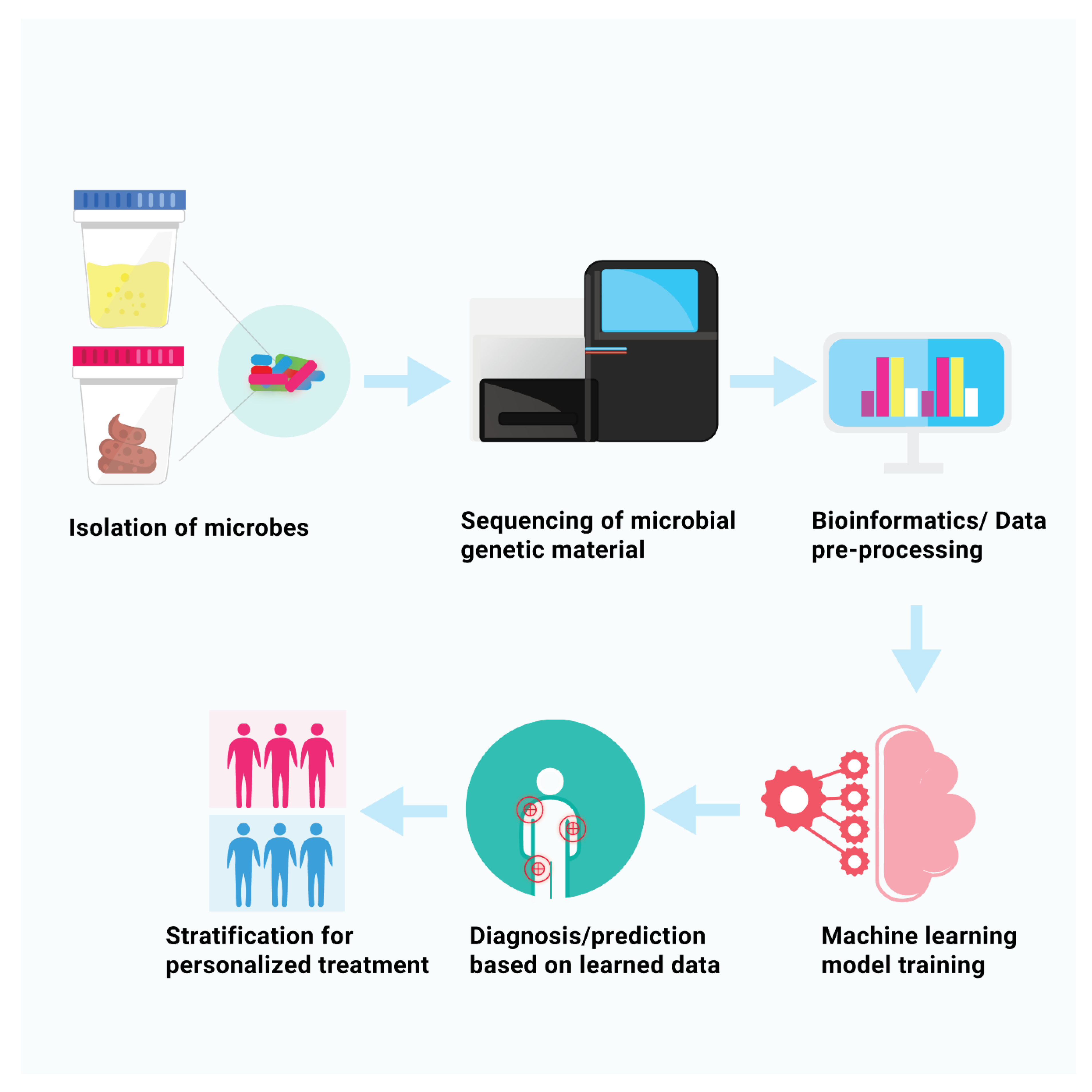
Figure 2.
Isolation and fragmentation of genetic material to produce raw readings is the first stage in the microbial sequencing process, which is used to identify microbes. (A) Amplicon technology begins with the extraction of genetic material and then amplifies DNA. Clean amplicon reads can be generated by first using amplicon sequencing libraries to add barcodes to the ends of raw amplicons, followed by the removal of low-quality amplicons and chimera sequencing. Then, depending on sequence dissimilarity or dissimilarity, the sequenced reads are projected to Operational Taxonomic Units (OTUs) or the Amplicon sequence variant (ASV) technique, and the obtained OTUs are given a taxonomic profile by comparing them to reference databases. (B) To prepare the sequencing library in shotgun metagenomics, DNA is first extracted, then fragmented. Quality inspection of the raw reads is the first stage since clean data is essential for Shotgun sequencing analysis. In cleaning stage, low-quality reads, host DNA sequences, primers, and adapter contaminations are removed from the raw sequencing data. After this, shotgun analysis can be performed with reference-based or assembly-based techniques. Clean readings are mapped using the reference-based technique to curated databases of genomic sequencing to get Taxonomic classification. In contrast, the assembly-based approach groups comparable sequences into contigs, which are then clustered into OTUs or contig bins (binning). The following phase, refinement, entails the discovery of possible microbial genes and the elimination of redundant genes. (C) Table data with taxonomic profile can be projected to machine learning for building diagnostic model and biomarker selection where data split into training and test set and model build on using training data and evaluated on test data.
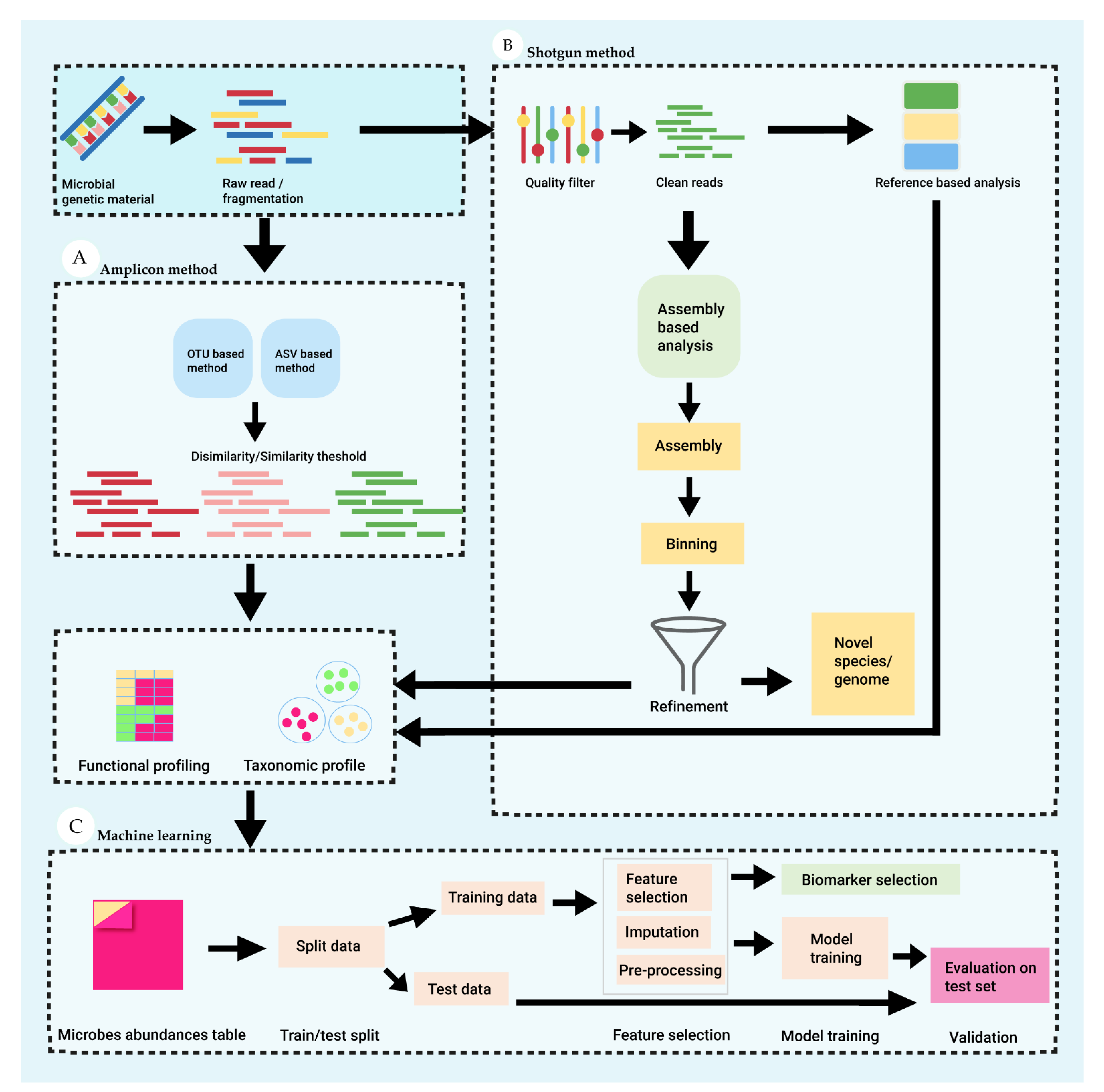
Figure 3.
Types of supervised learning based dimension reduction techniques.
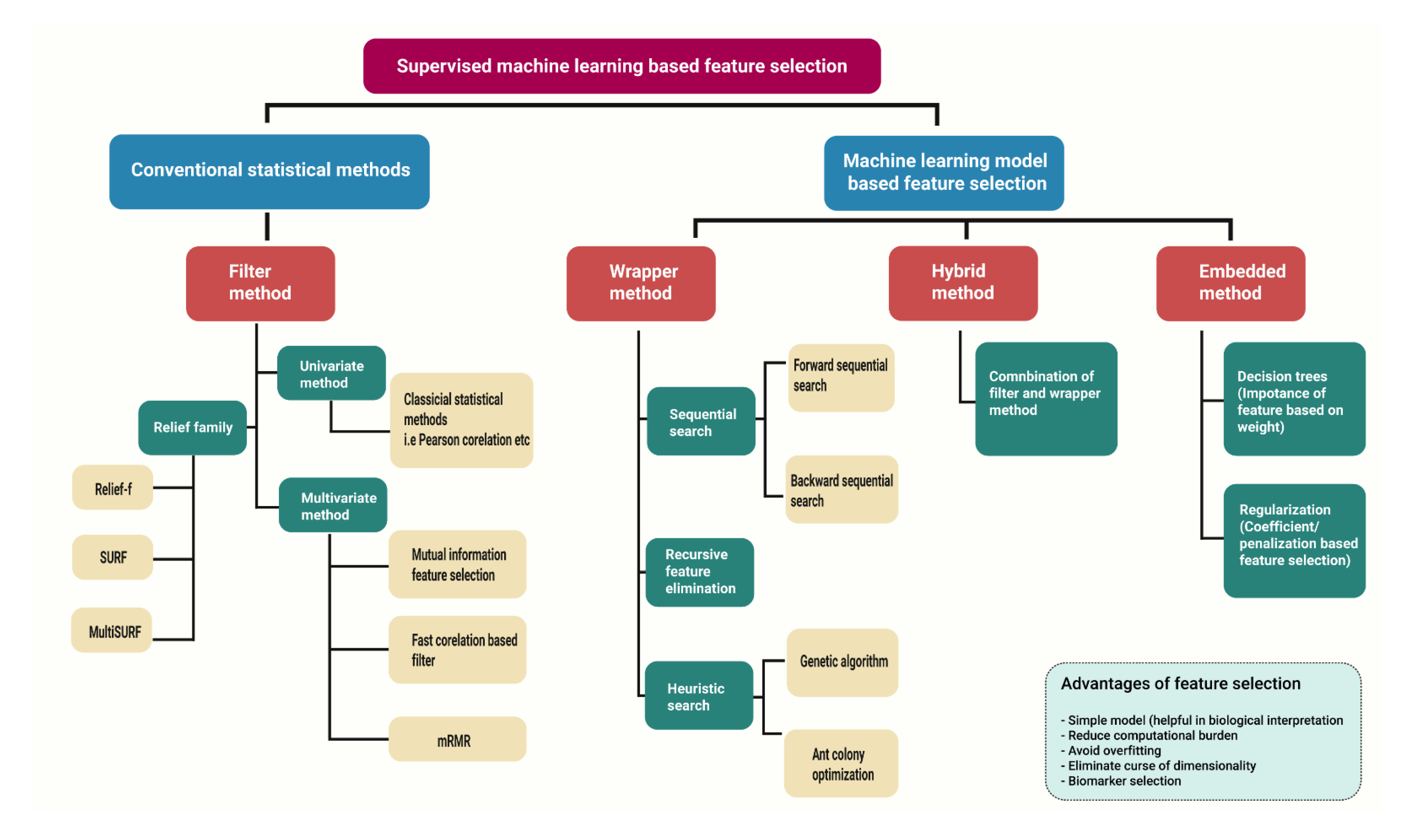
Figure 4.
Supervised machine learning algorithms for linear and non-linear task.
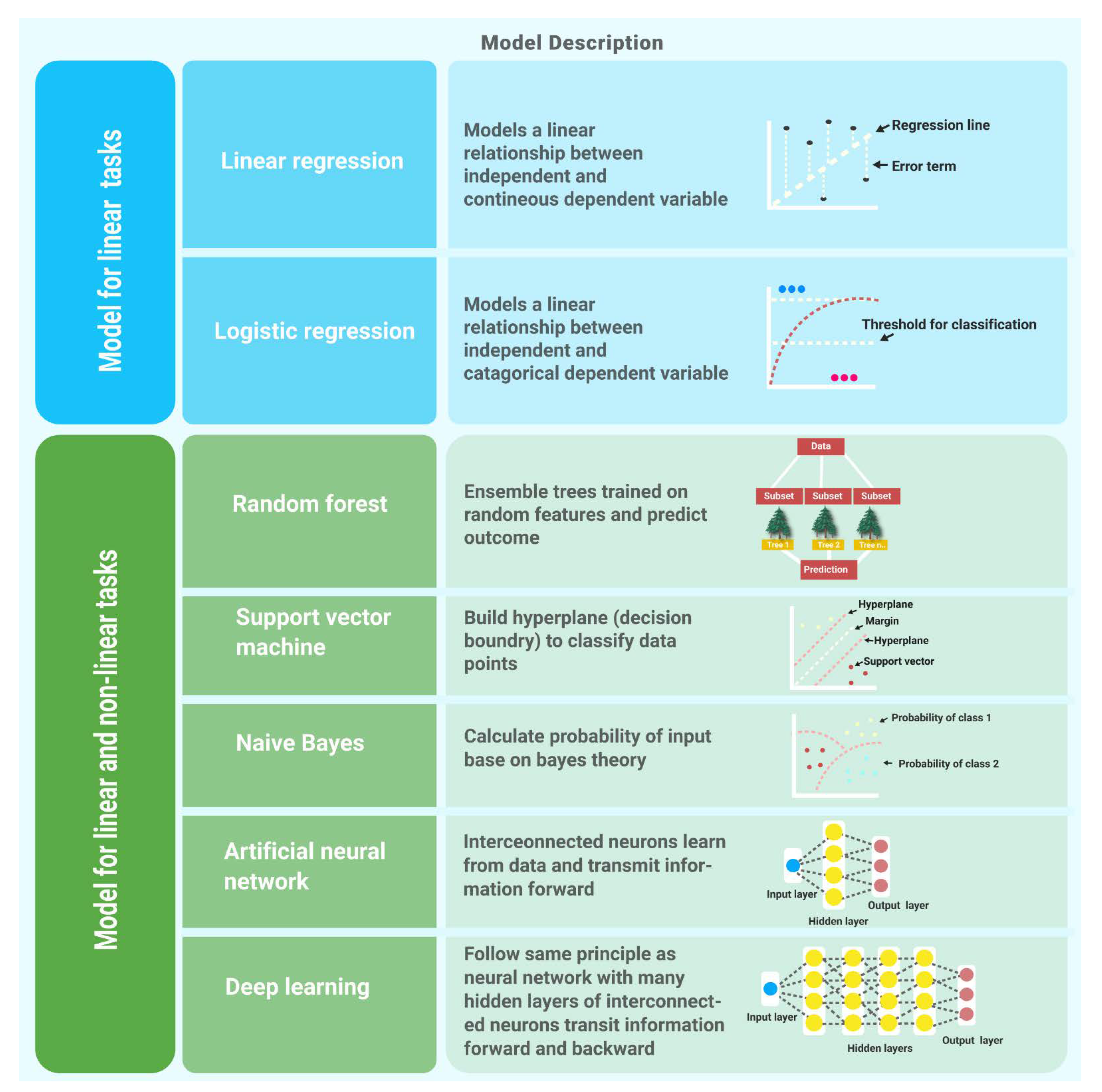

Table 1.
Advantages and disadvantages of amplicon and shotgun microbial sequencing methods.
| Methods | Advantages | Disadvantages |
|---|---|---|
| Amplicon sequencings | Great depth | Uneven amplification |
| More precise | Focus on specific fragment of genes (rRNA/ITS sequencing) | |
| Sequence a specific region (16s-, or 18s- rRNA) | Low enough resolution for species/subspecies identification-OTUs instead | |
| ITS and entire operon introduce more info | Not assess microbe’s function directly | |
| Shotgun sequencing | Theoretically sequence 100% of specimen | Rarely sequence everything of specimen |
| Greater resolution to genetic content | Sequence host/contaminant DNA | |
| Assess functional profiling | Produce very complex dataset | |
| Identify novel organisms/genes/genomic features | Costly | |
| Sequence host/contaminant DNA |
Table 2.
Dimension reduction techniques with advantages and disadvantages along with subtypes.
| Feature selection methods |
Subtype | Advantage | Disadvantage | Examples |
|---|---|---|---|---|
| Filter method | Univariate | Computational inexpensive High efficacy Scalable Independent of any classifier |
Multi-collinearity Lack of interaction of feature with classifier |
Fisher’s exact test |
| χ2 test, | ||||
| Information gain | ||||
| Euclidean distance | ||||
| Mann-Whitney U test | ||||
| Multivariate | Feature dependencies Independent of any classifier High efficacy |
Computational expensive in comparison with univariate Lack of interaction of features with classifier |
Minimal-redundancy-maximal-relevance (mRMR) | |
| Fast correlation-based filter (FCBF) | ||||
| Mutual information feature selection (MIFS) | ||||
| Conditional mutual information maximization (CMIM) | ||||
| Relief based family | Can handle non-linear relationships. Computational efficient Interaction between variables |
Sensitivity to the choice of distance metric Sensitive to parameter tuning. Limited to nearest neighbors |
Relief-f | |
| MultiSURF | ||||
| SURF | ||||
| Wrapper method | Heuristically search approach. | Less prone to local optima | High risk of overfitting Computational expensive |
Genetic algorithm |
| Ant colony optimization | ||||
| Sequential search method | High performance in contrast to filter method Feature dependencies Feature interaction with classifiers |
High risk of overfitting Computational expensiveMore likely to stuck at local optima |
Sequential forward selection (SFS) | |
| Sequential backward selection (SBS) | ||||
| Recursive feature elimination | More robust against stuck in local optima then sequential methods. Can handle noisy data. Can remove multiple features with less accuracy |
Sensitive to hyperparameters Limited interpretability |
Recursive feature elimination with random forest | |
| Recursive feature elimination with SVM | ||||
| Recursive feature elimination with logistic regression | ||||
| Embedded method | Penalization/shrinkage-based feature selection. | More robust against stuck in local optima then sequential methods. Can handle noisy data. Can remove multiple features with less accuracy. More effective than wrapper method in handling noisy data and handling inter-correlation between variables. Automatic feature selection |
Sensitive to hyperparameters Limited interpretability Difficult to select optimal regularization strength or penalization type. Not robust again non-linear relationship between variable and class |
Lasso |
| Elastic net | ||||
| Weight-based feature selection | Robust against handling complex relationship between dependent and independent variable More interpretable than penalization-based models |
Sensitive to hyper-parameters Sensitive to non-linear relationship |
Decision tree | |
| Random forest | ||||
| Naïve Bayes | ||||
| Hybrid method | Filter and wrapper combination | Efficient in accuracy than filter method Less complexity in comparison to wrapper Robust for high dimensional data |
Classifier dependent Inherit wrapper techniques complexities (overfitting) |
Hybrid genetic algorithm |
| Hybrid ant colony | ||||
| Fuzz random forest |
Table 3.
Study of autoimmune diseases using metagenomics and supervised machine learning approaches.
Table 3.
Study of autoimmune diseases using metagenomics and supervised machine learning approaches.
| Disease | Input | Aim of the study | Feature selection Algorithm | Classifier | References |
|---|---|---|---|---|---|
| Different autoimmune diseases such as ulcerative colitis, Crohn’s disease, rheumatoid arthritis and multiple sclerosis. | 16s RNA sequencing | To compare the gut microbiome associated with different autoimmune diseases such as ulcerative colitis, Crohn’s disease, rheumatoid arthritis and multiple sclerosis. | Feature importance determined by Gini score using random forest | Random Forest | [74] |
| IBD | 16s RNA sequencing | To identify IBD-related microbial biomarkers | Principal component analysis (PCA) and principal coordinate analysis (PCoA) | Random Forest | [75] |
| IBD & Subtypes | 16s RNA sequencing | To discriminate IBD from non-IBD and distinguish IBD subtypes as well | Linear discriminant analysis | Random Forest, SVM radial kernel, NNET, EN | [76] |
| IBD | 16S rRNA sequencing | Assess the compositional differences of the gut microbiome associated with lifestyle, diet and environmental factors in the development of IBD | Feature importance determined by Gradient boosted trees t | Gradient boosted trees | [77] |
| Inflammatory bowel diseases subtypes | 16S rRNA sequencing | To distinguish IBD subtypes: ulcerative colitis (UC) from Crohn’s disease (CD). | Kruskal-Wallis Tests, Fast Correlation Based Filter for Feature Selection (FCBF), Linear decomposition model, Differential abundance | Random Forest, Generalized linear model (glmnet) | [78] |
| T1D | 16S rRNA sequencing | To determine the association of gut microbes in T1D onset in children | Embedded feature selection with random forest | Random forest | [79] |
| T1D | 16S rRNA sequencing | Identified a potential genus for T1D Classification | - | Glmnet, Random Forest | [80] |
| T1D | 16s RNA sequencing | Categorise risk factors associated with the development of type 1 diabetes in infants. | Wilcoxon test | SVM, Random Forest, Glmnet | [81] |
| rheumatoid arthritis, liver cirrhosis and type 2 diabetes | Shotgun metagenomics | To identify biomarkers for three different diseases by multiclass classification | mRMR. | Random forest, SVM, logistic regression, KNN, gradient boosting decision tree (GBDT), AdaBoost, and stochastic gradient descent (SGD) were employed in this study. | [82] |
| Colorectal cancer (CRC), Multiple sclerosis (MS), Juvenile idiopathic arthritis (JIA) | 16s RNA sequencing | To distinguish gut microbiome from six different diseases using multiclass classification | Forward feature selection, Backward feature elimination | KNN, SVM, Logistic model tree, Logiboost | [83] |
| Inflammatory bowel disease, Multiple sclerosis, Rheumatoid arthritis, and general autoimmune diseases. | Shotgun sequence and 16s rRNA sequence | Compare and classify each autoimmune diseases by using machine learning algorithms | RFE used for feature selection in the study | XGBoost, Random Forest, SVM Radial, Ridge regression were employed for classification | [20] |
| Grave’s disease | Shotgun metagenomic sequence | To investigate the relation between gut microbiota and Grave diseases with four layers data derived from shotgun metagenomics. | Wilcoxon rank-sum test, two-tailed | Random Forest | [84] |
| Rheumatoid arthritis | Shotgun metagenomic sequencing | To examine the gut microbiomes that are linked with the minimum clinically important improvement (MCII) in RA patients. | Multiple regression model | Deep neural network, Random Forest, SVM & Logistic regression | [85] |
Disclaimer/Publisher’s Note: The statements, opinions and data contained in all publications are solely those of the individual author(s) and contributor(s) and not of MDPI and/or the editor(s). MDPI and/or the editor(s) disclaim responsibility for any injury to people or property resulting from any ideas, methods, instructions or products referred to in the content. |
© 2023 by the authors. Licensee MDPI, Basel, Switzerland. This article is an open access article distributed under the terms and conditions of the Creative Commons Attribution (CC BY) license (http://creativecommons.org/licenses/by/4.0/).
Copyright: This open access article is published under a Creative Commons CC BY 4.0 license, which permit the free download, distribution, and reuse, provided that the author and preprint are cited in any reuse.


