
Submitted:
05 April 2023
Posted:
06 April 2023
You are already at the latest version
Abstract
In the context of intelligent and integrative lighting, in addition to the need for color quality and brightness, the non-visual effect is essential. This refers to the retinal ganglion cells (ipRGCs) and their function, first proposed in 1927. The melanopsin action spectrum has been published in CIE S 026/E: 2018 with the corresponding melanopic equivalent daylight (D65) illuminance (mEDI), melanopic daylight (D65) efficacy ratio (mDER) and 4 other parameters. Due to the importance of mEDI and mDER, this work synthesizes a simple computational model of mDER as the main research objective, based on a database of 4214 practical spectral power distributions (SPDs) of daylight, conventional, LED, and mixed light sources. In addition to the high correlation coefficient R2 of 0.96795 and the 97% confidence offset of 0.0067802, the feasibility of the mDER model in intelligent and integrated lighting applications has been extensively tested and validated. The uncertainty between the mEDI calculated directly from the spectra and that obtained by processing the RGB sensor and applying the mDER model has reached ± 3.3% after an appropriate matrixing process and proper illumination characterization combined with the successful mDER calculation model. This result opens the potential of low-cost RGB sensors for applications in intelligent and integrative lighting systems to optimize and compensate the non-visual effective parameter mEDI using daylight and artificial light in indoor spaces. The goal of the research on RGB sensors and the corresponding processing method are also presented and their feasibility is methodically demonstrated. A comprehensive investigation with a huge amount of color sensor sensitivities is necessary in a future work of other researches.
Keywords:
Non-visual effects of light
; Melanopic equivalent daylight (D65) illuminance
; mEDI
; Melanopic equivalent daylight (D65) efficacy ratio
; mDER
; Intelligent and integrated lighting
; mDER calculation model
; mEDI measurement
; mEDI determination
1. Introduction
The development of lighting technology from the beginning of the 20th century to the present can be roughly divided into three stages, some of which overlap. Until the end of the 20th century, with thermal radiators and discharge lamps as light sources, the first component of integrative HCL ("Human Centric Lighting") lighting technology was about "visual performance" (e.g. reaction time, contrast perception, reading speed, visual acuity) to enable visibility, improve work performance and minimize error rates in industrial processes, educational and healthcare facilities and offices, among others [2,3,4,5,6,7,8,9,10]. Since the 1970s and even more so since the mid-1990s, with the growing importance of education and the information society, the psychological effects of light (e.g. scene preference, room preference, user satisfaction, spatial perception, attractiveness and color preference) have become more and more important. Recent results of lighting, color and visual perception research lead to the results in Table 1 [10,11,12,13,14,15,16,17].
Since the beginning of the 21st century with the quantitative discovery of intrinsically photosensitive retinal ganglion cells (ipRGCs), other non-visual effects of light have been considered, such as circadian rhythm, hormone production and suppression, sleep quality, alertness, and mood. The overall picture of light effects on humans in the three contexts of "visual performance", "psychological light effects" and "non-visual light effects" is shown in Figure 1, attempting to describe a chain of signal processing from the optical and temporal input parameters to the light users with influencing parameters to the output parameters expressing the physiological, behavioral and human biological effects of light and lighting. In recent years, there has been a large amount of research and publications on non-visual lighting effects analyzed and reviewed in books and literature reviews [18,19,20,21]. In the majority of scientific publications cited in these reviews, the input parameters describing lighting conditions were photometric metrics (illuminance, luminance) and/or color temperature. In addition to the optimal lighting design of buildings and the development of modern luminaires according to the criteria of visual performance and psychological lighting effects, it is necessary to define suitable input parameters for the description of non-visual lighting effects, to determine their optimal values and to measure these parameters in a wide variety of applications in the laboratory and in the field. To achieve the above goal, the following three research questions for lighting research must be formulated in general terms:
- Which input parameters can be used to describe the non-visual effects of light in their variety of manifestations (alertness, sleep quality, hormone production and suppression, phase shift)?
- What values of these input variables are currently considered in the literature to be minimum, maximum, or optimal?
- Which measuring devices, sensor systems and measuring methods can be used to measure the input quantities for the non-visual lighting effects and process them in the context of smart lighting in the course of the control and regulation of LED or OLED luminaires on the basis of the definition of personal and room-specific applications?
To define the parameters of non-visual lighting effects (Research Question 1), the International Commission on Illumination (CIE) and scientists in the fields of neurophysiology, sleep research, and lighting technology have recently made efforts to find effective parameters based on the evaluation of the five photoreceptor signals (LMS cones, rods, and ipRGC cells) and the corresponding calculation tool [22]. This scientific process resulted in the definitions of "Melanopic Equivalent Daylight (D65) Illuminance (mEDI)" and "Melanopic Daylight (D65) Efficacy Ratio (mDER)". These definitions have been recognized and used by international experts for several years and form the basis of Section 2 of this paper.
To answer Research Question 2, recognized international sleep researchers and neuroscientists in 2022 made some recommendations regarding non-visual light effects, physiological aspects, sleep and wakefulness based on their literature reviews [23]. Physiological aspects included hormonal regulation cycles, heart rate, core body temperature, and certain brain activities. The main findings were as follows,
- (a)
- “Daytime light recommendations for indoor environments: Throughout the daytime, the recommended minimum melanopic EDI is 250 lux at the eye measured in the vertical plane at approximately 1.2 m height (i.e., vertical illuminance at eye level when seated)”.
- (b)
- “Evening light recommendations for residential and other indoor environments: During the evening, starting at least 3 hours before bedtime, the recommended maximum melanopic EDI is 10 lux measured at the eye in the vertical plane approximately 1.2 m height. To help achieve this, where possible, the white light should have a spectrum depleted in short wavelengths close to the peak of the melanopic action spectrum”.
- (c)
- “Nighttime light recommendations for the sleep environment: The sleep environment should be as dark as possible. The recommended maximum ambient melanopic EDI is 1 lux measured at the eye”.
The first recommendation, with a minimum value of "melanopic EDI = Melanopic Equivalent Daylight (D65) Illuminance, mEDI" of 250 lx measured vertically at the observer’s eye, is relevant and of great interest for the professional sector during the day (offices, industrial halls, educational and health facilities). The other two recommendations are for the dark hours in the home.
For the solution of Research Question 3 "Determination and measurement of input parameters for non-visual lighting effects", which builds the focus of this present paper, two application areas can be targeted:
- Determination and measurement of non-visual parameters after completion of the new lighting installations and comparison with the specifications of the previous lighting design; or verification of the results of the development of new luminaires for HCL lighting in the lighting laboratory or in the field. For this purpose, absolute spectroradiometers for spectral radiance or spectral irradiance are used to calculate the parameters and at different locations in the building. These two non-visual parameters cannot be measured directly with integral colorimeters and illuminance-luminance meters.
- Control or regulation of modern semiconductor based lights (LED - OLED) and window systems (daylight systems) with the help of sensors in the room (e.g. presence sensors, position sensors, light and color sensors). In order to achieve a predefined value of non-visual parameters such as at a specific location in the room (e.g. in the center of the room or at locations further away from the windows), taking into account dynamically changing weather conditions and the whereabouts of the room users, in practice relatively inexpensive but sufficiently accurate optical sensors ( sensors) are required. The goal is to obtain not only the target photometric and colorimetric parameters such as illuminance (in lx), chromaticity coordinates (x, y, z) or correlated color temperature ( in K), but also the non-visual parameters and . The principle of this Smart Lighting concept using color sensors is illustrated in Figure 2. The methods for measuring non-visual parameters with low-cost but well-qualified color sensors are the content of Section 3 and Section 4 and the focus of this paper.
The notations "integrative lighting" and "human-centric-lighting" used in this publication have been defined by the ISO/CIE publication [24] and mean a lighting concept and practice that integrates both visual and non-visual effects and produces physiological psychological benefits for light users. The terms "smart lighting" or "intelligent lighting" are used in the same way and mean a framework that combines the above-mentioned integrative lighting as a goal and content of lighting practice with the technological aspects of lighting (signal communication, Internet of Things, sensor systems, control electronics, software including the methods of artificial intelligence, LED luminaires), taking into account the individual needs of light users in dependence on weather conditions, individual human characteristics, time and context of application.
2. Definition of non-visual input parameters [1]
The extensive mathematical treatment and definition of the non-visual input parameters is described in detail in the CIE publication S 026/E:2018 "CIE System for Metrology of Optical Radiation for ipRGC-Influenced Responses to Light" [1] and is summarized in this paper. The purpose of this CIE publication is to define spectral response curves, quantities and metrics to describe optical radiation for each of the five photoreceptors in the human eye that may contribute to nonvisual processes. The spectral sensitivity functions of the five receptor types are specified as follows (see Figure 3):
- S-cone-opic,
- M-cone-opic,
- L-cone-opic,
- Rhodopic, , rods
- Melanopic, , ipRGCs
The CIE defined the -opic quantities in Table 2 by the aid of the spectral sensitivities in Figure 3, the spectral radiant flux , the spectral radiance and the spectral irradiance ( represents one of the five photoreceptor types).
From this, further parameters can be derived for assessing the non-visual effect of light, where is the spectral sensitivity function of one of the five receptor types, is the known photometric radiation equivalent (= 683.002 lm/W) and is the spectrum of standard daylight type D65, see the equations 4 - 5. The quantity "" is the -opic - Efficacy of the luminous radiation.
Equation 5 is similar to Equation (3.7) on Page 5 of [1]. For melanopic efficacy ( = mel), the parameter value equals 1.3262 mW/lm. So the parameters and can be set up as shown in Table 3. If one wants to interpret the meaning of or for lighting engineering, there are two main aspects:
The melanopically effective parameters and can be calculated from the equations 15, 5, 16 and 19 if the spectral irradiance is known from a spectroradiometric measurement. The key question in this publication is whether these two parameters can also be determined with sufficient accuracy in practical lighting technology using a well-characterized and inexpensive sensor in the sense of intelligent lighting technology (smart lighting). Section 3 deals with the description of the sensor and how the sensor signals can be transformed into tristimulus values ( ) and into chromaticity coordinates () by means of a comprehensive spectral analysis.
3. color sensors: Characterization and Signal transformation
After the definition of the non-visual input parameters [1] in Section 2, we can understand the main concepts and mathematical forms of and . In Section 4, the prediction of a simple computational model of the non-visual quantities and will be carried out, as well as the verification of the feasibility of a sensor using this model will be implemented to check the synthesized prediction model for lighting applications. And it is also to confirm that the model is not only in the mathematical calculations, but can be applied in the lighting systems with low-cost color sensors. Therefore, Section 3 must attempt to describe color sensors, their characterization, and appropriate signal transformation techniques. This section serves as a link between Section 2 and Section 4, as well as to balance the essential material for the verification of the prediction model using a color sensor as an example in Section 4 later. As a demonstration of the methodology for processing RGB sensors, it is not necessary to collect all color sensor sensitivities, synthesize and compare them, but the most important thing here is to prove that the methodology can work well in this approach. Consequently, the future work can be implemented more comprehensively for different color sensor families by other researches.
3.1. Characterisation of color sensors
Color sensors (see Figure 4) are arrays of individual sensors or a group of sensors based on semiconductors with silicon as the semiconductor material, most commonly used for the visible spectral range between 380 nm and 780 nm.
In order to generate the corresponding spectral sensitivity curves of the individual color channels in the red, green and blue range (so-called . channels), optical color filters based on thin-film technology (interference filters), absorption glass filters or color varnishes are microstructured and applied to the respective silicon sensor. For the correct spatial evaluation of the optical radiation according to the cosine law, a so-called cos prefix (usually a small diffuser plate made of optical scattering materials) is applied to the sensor. The photons of each wavelength are absorbed by the sensor and photon currents are generated, which are then converted into voltages in an amplifier circuit. These voltages are then digitized in different bit depths (8 bits, 12 bits, 16 bits) by an A/D converter (analog-digital). The spectral sensitivity of each color channel R - G - B is therefore made up of the components shown in the equations 10, 11 and 12.
with,
- is the spectral sensitivity of the silicon sensor;
- is the spectral transmittance of the cos diffusor;
- is the spectral transmittance of the color filter layer for the respective color channel i = R, G, B;
- , , are absolute factors to account for current-to-voltage conversion and voltage digitization;
- are output signals (analog or digital) of the respective R - G - B color sensor at wavelength .
If a certain spectral irradiance ) is present on the sensor, three corresponding output signals R, G and B are generated in the three color channels R, G and B (see the equations 13, 14 and 15).
For the calculation of the channel signals it is therefore necessary to know or to determine the spectral sensitivity function of each individual color channel R, G, B by laboratory measurements. The spectral apparatus for determining the spectral sensitivity of the semiconductor sensors in the authors’ light laboratory (see Figure 5) therefore consists of a high-intensity xenon ultrahigh-pressure lamp, a grating monochromator (spectral half-width = 2 nm, spectral measuring steps for the entire spectrum between 380 nm and 780 nm, = 2 nm), and an integrating sphere for homogenizing the quasi-monochromatic radiation coming out of the monochromator. The color sensor and a known calibrated reference sensor are located at two different locations on the inner wall of the sphere behind a shutter.
During the spectral measurement of the sensor, one can determine the spectral sensitivity for the red color channel, for example, according to Equation 16.
With as the output signal of the red color channel and as the spectral irradiance at the inner wall of the sphere when the monochromator is set to the wavelength , which in turn can be determined from the measured output photocurrent and the known spectral sensitivity of the reference sensor , we can write Equation 17.
The absolute spectral sensitivity of each color channel R, G, B can be determined from the equations 16 and 17.
Figure 6 and Figure 7 show examples of the spectral response curves of some color sensors measured in the authors’ light laboratory. In Figure 6, the two data sets of the same type, SeS1 and SeS2, differ by the different peak heights of the R channel and by the different slopes of the G and B curves, because the two sensors and come from different production sets. The and spectral sensitivity curves in Figure 6 are fundamentally different from the spectral sensitivity curves of the color sensor type in Figure 7.
3.2. Method of signal transformation from to
Figure 6 and Figure 7 show that the curves of the real color sensors differ more or less strongly from the curves of the CIE color matching function for a field of view of 2° [25]. In order to obtain the tristimulus values, the generated signals must be transformed into digital form using matrixing (Equation 18).
Since the sensor technology, the amplification electronics and the A/D conversion often have a more or less pronounced non-linear behavior, it may be necessary to use different matrixing types from 3 x 3 to 3 x 22, see Table 4.
If the sensor electronics are linear and the spectral response curves have a similar relative shape to the color matching functions or sensitivity spectra of the retinal photoreceptors, 3 x 3 to 3 x 8 matrices will yield contributions from signals as a function of the first term. The more the sensor electronics deviate from linear behavior and the shape of the spectral curves of the real sensors deviate from the color matching functions, matrices with contributions in quadratic or cubic functions (see Table 4) should be set up. The procedure for finding the optimal matrix based on the chromaticity difference is shown in Figure 8.
The goal of the optimization is to get the chromaticity (x, y, z) of the sensor as close as possible to that derived from the CIE calculation. Instead of working with the non-uniform xy color diagram, it is better to work with the more uniform u’v’ diagram (CIE, 1964). Bieske [27] had shown in her dissertation that when is less than , the color difference is not perceived by the subjects. From to the color difference can be perceived but is still acceptable. If this value is higher than , the color difference is unacceptable to the subjects. Based on this scientific contribution, the optimization with not only gives the best z-value, but can also be directly checked and compared with the obtained perception thresholds.
3.3. Matrix transformation in practice, verification with a real color sensor
For the color sensor type whose spectral sensitivity curves are shown in Figure 7, the optimization processes are carried out according to the scheme in Figure 8 with a series of matrix types from 3 x 3 to 3 x 22 with 9 different lamp spectra (as a training set). These nine lamp spectra are tabulated in Table 5 and shown in Figure 9. The illuminance for the optimization of the matrix was chosen to be = 750 lx. In this training set, the following lamp types were selected to reflect the variety of types used in practice today: fluorescent lamps between 2640 K and 4423 K with many spectral lines (see Figure 9), a halogen incandescent lamp, two phosphor-converted white LEDs, and a combination of LEDs and warm white LEDs (RGBWW4500K).
The calculation with different matrix types and with individual lamp spectra yields color differences of varying magnitude, with the 3 x 3 matrix form yielding the smallest color difference (see Table 6). Optimization with more lamp types did not bring any significant improvement in this case. The final 3 x 3 optimized matrix for the transformation from to as well as the formula for the calculation of the illuminance from the signals are shown in Table 7.
To verify the prediction quality of the formula in Table 7, 13 lamp spectra were selected in the next step. These were white phosphor converted LEDs (pc-LEDs) and a mixture of daylight spectra with white phosphor converted LEDs (TL-pc-LEDs), as is often the case in practical indoor lighting (see Figure 10). The illuminance was again set to 750 lx. The results of the check are shown in Table 8. From Table 8 it can be seen that,
- (a)
- The deviation of the illuminances, once calculated directly from the lamp spectra and once via the color sensor signals and via the formula in Table 7, is below 0.65% in percentage terms;
- (b)
- For the majority of pc-LEDs and for the combinations daylight-white LEDs, the chromaticity difference is in a small or moderately small range from the point of view of practical lighting technology. An exception is the spectrum R12GB12-5000 K (green curve in Figure 10) with the three distinct peaks of the three LEDs (B around 455 nm, G around 525 nm, R around 660 nm). There, the color difference is .
For the case of daylight spectra a special matrix was found and described in Table 9. For the investigated color sensor type, 185 daylight spectra were measured absolutely on a sunny summer day (August 19th, 2020 in Darmstadt, Central Europe) from 6:32:00 in the early morning to 20:35:32 in the late evening. The chromaticity and illuminance values were calculated and used as a training set for the matrix. The largest color difference with a 3 x 3 matrix was found to be in the last minutes of the evening before sunset, when the correlated color temperature was very high, approximately in the range of 17000 K on the day of measurement. Most of the color differences were well below this value.
To verify the 3 x 3 matrix for daylight, 24 daylight spectra measured on a rainy day (September 23rd, 2020 in Darmstadt, Germany) were considered. The verification results are shown in Table 10 with 9 out of 24 spectra as examples. There the chromaticities and illuminances determined from the measured spectra are compared with the data obtained by matrixing the color sensor (processed data). The calculated color difference is very small and lies in the range of .
The determination of the optimal matrix for the transformation of sensor signals into values and the illuminance described so far, as well as the verification results with an actual color sensor type, prove that it is possible to obtain the colorimetric and photometric values , and with relatively good results in the sense of a reliable, relatively accurate and adaptive lighting technology using inexpensive and commercially available color sensors. The next section deals with the accurate determination of the non-visual input quantities and indoors (daylight and artificial light combined or separated) and outdoors during the day (with daylight only) from the tristimulus values and the illuminance of a qualified color sensor, because in practical lighting technology a spectroradiometer is often too expensive and too cumbersome to handle.
4. Prediction of a simple computational model of the non-visual quantity and verification of the feasibility of a sensor using this model
Once the matrices for electric light sources and for daylight spectra have been optimized and found, the tristimulus values , the chromaticity coordinates as well as the color temperature and the illuminance can be obtained from the color sensors used (see the Table 7, Table 8, Table 9 and Table 10). To obtain the melanopic equivalent daylight illuminance , one only needs to know the value of and the illuminance (in lx) according to equation 17, where the illuminance can be formed from the signals (see formula in the Table 7 and Table 9) and is therefore determinable. Consequently, the most important task is to calculate the dimensionless input quantity (see Equation 19) from the chromaticity coordinates x, y, z (z turned out to be the most predictive, so it will be used).
For this transformation from z to , a large number of measured and simulated light source spectra were analyzed (see Table 11). The first 4 light source groups are real measured light sources from thermal radiators (28 light sources), compact and linear fluorescent lamps (252 light sources), different LED configurations (419 light sources) and 185 measured daylight spectra. These 884 light source spectra are shown in Figure 12. In order to simulate the combination of daylight with white LEDs or daylight with white fluorescent lamps, which can correspond to the lighting conditions of interiors with white LEDs or white fluorescent lamps with windows over a longer period of use, the authors of this paper took 185 measured daylight spectra and mixed them with a market-typical white LED spectrum or with a typical fluorescent lamp spectrum in 9 different mixing ratios from 10% to 90%. This can be seen in Figure 13 for the case of combining daylight spectra with white LEDs. For the fluorescent lamps it is similar, so a graphical representation of the mixing spectra is omitted here. The 185 daylight spectra with 9 mixing ratios each result in 1665 simulated spectra each for LED and fluorescent lamps (185 x 9 = 1665).
Using the 4214 light source spectra summarized in Table 11, 4214 values and 4214 z values were calculated, from which their relation was determined. The formula for is given in Equation 25.
The parameters a, b, c and d for the fitting function and the correlation coefficients are given in Table 12. The course of the correlation between (ordinate) and the chromaticity coordinate z (abscissa) is shown in Figure 14, where the fitting function follows the green course of the curve.
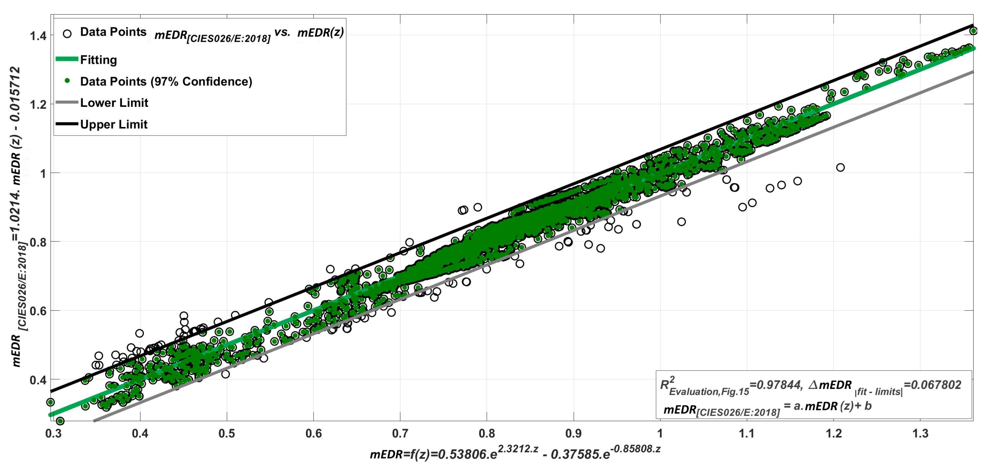
To check the predictive quality of Equation 25 and the transformation from z to , the 4214 spectra in Table 11 were first used to calculate the 4214 values from the spectra themselves (denoted as ) and then another 4214 values indirectly via Equation 25 with z as the independent variable (denoted as ), see Figure 15. The goodness of fit () was 0.97844, the linear constants are 1.0214 and -0.05712. Compared to the ideal constants of 1 and 0, the quality of the fit is very good.
To verify the quality of the characterization of the color sensor under test (see Figure 7), the quality of the "matrixing" in the transformation from to and (see Table 7) and the quality of the transformation from z to (see Equation 25) and finally the calculation of (see the equations 16 and 19), we set each of the 13 light source spectra in Figure 10 to 750 lx. From these 13 spectra, the chromaticity coordinates x and y and the quantities , , , , and were calculated. They are listed in Table 13. For these 13 spectra, the chromaticity coordinates and , the value of , and the values and were also calculated from the color sensor values by matrixing and transforming z to and , respectively. The maximum relative deviations (in %) and (in %) were found to be in the range of ± 3.3%.
5. Conclusion and Discussion
In indoor lighting technology, including daylight components during the day, the daily task is to evaluate the lighting systems after completion of the building or after reconstruction, to assess the photometric and colorimetric quality of the newly developed interior luminaires and, in the context of intelligent lighting (smart lighting, HCL lighting, integrative lighting), to adaptively control the lighting systems in order to provide the room users with the best visual and non-visual conditions and room atmosphere at all times. In addition to the criteria of visual performance according to current national and international standards (e.g. EN DIN 12464 [10]), aspects of psychological-emotional lighting effects as well as the evaluation and adaptive control of lighting systems according to non-visual quality characteristics should be considered. For this purpose, non-visual input parameters such as and need to be measured and processed with sufficient accuracy, reliability and reasonable effort.
Existing illuminance meters, luminance meters, color and luminance cameras, and small portable colorimeters are currently only capable of measuring photometric quantities such as illuminance Ev, luminance , colorimetric parameters such as chromaticity coordinates , and correlated color temperature (). To measure the non-visual parameters, a transformation is needed to convert the tristimulus values to the non-visual parameters, and a sensor platform is needed to convert the sensor signals to the tristimulus values and (in lx).
The authors of this paper have characterized some exemplary color sensors on the basis of laboratory measurements, calculations and optimizations, by creating one or more matrices for optimal transformation of sensor signals to the tristimulus values, and then, on the basis of extensive calculations, have achieved a transformation of the chromaticity coordinate z to and, via , also to with good accuracy. This work and the methodology described therein allow an accurate and financially justifiable assessment of lighting installations according to non-visual criteria, which will become increasingly important in the coming decades.
The goal of this paper was to provide a framework and a general methodology for using commercially available sensors and qualifying them for measuring the metrics for non-visual effects. The results have some limitations because only one type of sensor was used in this work. Other sensor types may have different spectral, optical, and electronic characteristics with different dark currents, signal-to-noise ratios, and crosstalk effects, which should require different forms of matrices (e.g., matrices with higher-order signals). Further studies are planned to compare the accuracies of several commercial sensor types with the measurement results of an absolute spectroradiometer for different test conditions (e.g. outdoor and indoor lighting conditions with different mixing ratios of daylight and artificial light sources).

Table 13.
Chromaticity difference for different matrix types for the lamp types of the training set
| Name | pcLED-WWG6 | pcLED-WWG3 | pcLED-WWVG1 | pcLED-WWVG3 | pcLED-WWVG8 | pcLED-WWEX4 | pcLED-NWVG1 | pcLED-NWEXCV2 | pcLED-CWVG1 | pcLED-CWEX2 | R12GB12-5000 K | TL-pcLED-30% | TL-pcLED-60% |
|---|---|---|---|---|---|---|---|---|---|---|---|---|---|
| CCT (K) | 3134 | 2801 | 3105 | 2782 | 2998 | 2969 | 4614 | 3942 | 5112 | 5059 | 5001 | 4391 | 4571 |
| CIE Ra | 80.27 | 84.06 | 85.63 | 88.10 | 90.56 | 94.41 | 90.91 | 93.09 | 90.06 | 95.99 | 89.73 | 89.85 | 92.48 |
| x | 0.4285 | 0.4434 | 0.4217 | 0.4557 | 0.4352 | 0.4252 | 0.3569 | 0.3764 | 0.3424 | 0.3439 | 0.3449 | 0.3644 | 0.3581 |
| y | 0.4025 | 0.3929 | 0.3841 | 0.4135 | 0.4003 | 0.3765 | 0.3608 | 0.3550 | 0.3537 | 0.3557 | 0.3495 | 0.3650 | 0.3605 |
| Ev (lx) | 750 | 750 | 750 | 750 | 750 | 750 | 750 | 750 | 750 | 750 | 750 | 750 | 750 |
| 0.47 | 0.46 | 0.51 | 0.40 | 0.48 | 0.53 | 0.75 | 0.67 | 0.81 | 0.83 | 0.83 | 0.71 | 0.75 | |
| 349.06 | 347.67 | 383.55 | 300.60 | 358.27 | 395.93 | 562.91 | 500.06 | 610.69 | 625.10 | 625.79 | 532.40 | 563.22 | |
| (lx) | 750.35 | 752.29 | 752.54 | 750.90 | 751.14 | 754.17 | 751.40 | 754.79 | 751.31 | 750.01 | 747.60 | 751.94 | 751.91 |
| 0.4285 | 0.4434 | 0.4217 | 0.4557 | 0.4352 | 0.4252 | 0.3546 | 0.3779 | 0.3361 | 0.3368 | 0.3319 | 0.3665 | 0.3572 | |
| 0.4025 | 0.3929 | 0.3841 | 0.4135 | 0.4003 | 0.3765 | 0.3643 | 0.3698 | 0.3545 | 0.3571 | 0.3529 | 0.3696 | 0.3640 | |
| 0.47 | 0.46 | 0.53 | 0.39 | 0.46 | 0.54 | 0.74 | 0.66 | 0.82 | 0.81 | 0.83 | 0.69 | 0.73 | |
| 353.75 | 346.28 | 396.00 | 295.19 | 346.92 | 403.79 | 554.58 | 500.85 | 612.52 | 604.47 | 621.78 | 521.19 | 550.29 | |
| 3.15 | 8.76 | 4.50 | 5.32 | 10.1 | 2.42 | 2.51 | |||||||
| in % | 0.05 | 0.31 | 0.34 | 0.12 | 0.15 | 0.56 | 0.19 | 0.64 | 0.17 | 0.00 | -0.32 | 0.26 | 0.25 |
| in % | 1.3 | -0.7 | 2.9 | -1.9 | -3.3 | 1.4 | -1.7 | -0.5 | 0.1 | -3.3 | -0.3 | -2.4 | -2.5 |
| in % | 1.35 | 0.40 | 3.25 | 1.80 | 3.17 | 1.99 | 1.48 | 0.16 | 0.30 | 3.30 | 0.64 | 2.10 | 2.30 |
Author Contributions
Conceptualization, V.Q.T., P.B. and T.Q.K.; Data curation, V.Q.T.; Formal analysis, V.Q.T., P.B.; Methodology, Q.V.T. and T.Q.K; Software, V.Q.T.; Supervision, T.Q.K.; Validation, V.Q.T and P.B.; Visualization, V.Q.T.; Writing—original draft, V.Q.T. and P.B.; Writing—review & editing, V.Q.T., P.B, and T.Q.K; Project administration, V.Q.T. All authors have read and agreed to the published version of the manuscript.
Funding
This work received no specific grant from any funding agency in the public, commercial, or not-for-profit sectors. The publication of the manuscript is supported by the Open Access Publishing Fund of the Technical University of Darmstadt.
Institutional Review Board Statement
Not applicable
Informed Consent Statement
Not applicable
Data Availability Statement
All data generated or analyzed to support the findings of the present study are included this article. The raw data can be obtained from the authors, upon reasonable request.
Conflicts of Interest
The authors declare no conflict of interest.
References
- Commission International de l’Eclairage (CIE). CIE S 026/E: 2018: CIE System for Metrology of Optical Radiation for ipRGC-Influenced Responses to Light. Vienna, Austria: CIE Central Bureau, 2018. [CrossRef]
- Rea, M.S.; Ouellette, M.J. Relative visual performance: A basis for application; Vol. 23, SAGE Publications Sage UK: London, England, 1991; pp. 135–144. [Google Scholar] [CrossRef]
- Rea, M.S.; Ouellette, M.J. Visual performance using reaction times. Lighting Research & Technology 1988, 20, 139–153. [Google Scholar] [CrossRef]
- Weston, H.C. ; others. The Relation between Illumination and Visual Efficiency-The Effect of Brightness Contrast. The Relation between Illumination and Visual Efficiency-The Effect of Brightness Contrast. 1945.
- Boyce, P.R. Human factors in lighting; Crc press, 2014. [CrossRef]
- Lindner, H. Beleuchtungsstärke und Arbeitsleistung–Systematik experimenteller Grundlagen (Illumination levels and work performance–systematic experimental principles). Zeitschrift für die gesamte Hygiene und ihre Grenzgebiete (Journal of hygiene and related disciplines) 21 1975, pp. 101–107.
- Schmidt-Clausen, H.J.; Finsterer, H. Beleuchtung eines Arbeitsplatzes mit erhöhten Anforderungen im Bereich der Elektronik und Feinmechanik; Wirtschaftsverl. NW, 1989.
- Blackwell, H.R. Contrast thresholds of the human eye. Josa 1946, 36, 624–643. [Google Scholar] [CrossRef] [PubMed]
- Commission Internationale de l’Éclairage (CIE). An analytical model for describing the influence of lighting parameters upon visual performance. CIE-Publication 1981.
- DIN-EN-12464-1-2021-11. Licht und Beleuchtung – Beleuchtung von Arbeitsstaetten, Teil 1: Arbeitsstaetten in Innenraeumen, 2021.
- Houser, K.W.; Tiller, D.K.; Bernecker, C.A.; Mistrick, R. The subjective response to linear fluorescent direct/indirect lighting systems. Lighting Research & Technology 2002, 34, 243–260. [Google Scholar] [CrossRef]
- Tops, M.; Tenner, A.; Van Den Beld, G.; Begemann, S. The effect of the length of continuous presence on the preferred illuminance in offices. Proceedings CIBSE Lighting Conference, 1998.
- Juslén, H. Lighting, productivity and preferred illuminances: field studies in the industrial environment; Helsinki University of Technology Helsinki, 2007.
- Moosmann, C. Visueller Komfort und Tageslicht am Bueroarbeitsplatz: Eine Felduntersuchung in neun Gebaeuden; KIT Scientific Publishing, 2015.
- Park, B.C.; Chang, J.H.; Kim, Y.S.; Jeong, J.W.; Choi, A.S. A study on the subjective response for corrected colour temperature conditions in a specific space. Indoor and Built Environment 2010, 19, 623–637. [Google Scholar] [CrossRef]
- Lee, C.W.; Kim, J.H. Effect of LED lighting illuminance and correlated color temperature on working memory. International Journal of Optics 2020, 2020, 1–7. [Google Scholar] [CrossRef]
- Fleischer, S.E. Die psychologische Wirkung veränderlicher Kunstlichtsituationen auf den Menschen. PhD thesis, ETH Zurich, 2001.
- Khanh, T., Q.; Bodrogi, P.; Trinh, Q. V. Khanh; T. Q.; Bodrogi, P.; Trinh, Q. V. Beleuchtung in Innenräumen – Human Centric Integrative Lighting Technologie, Wahrnehmung, nichtvisuelle Effekte; Wiley-VCH (Verlag), 2022.
- Lok, R.; Smolders, K.C.; Beersma, D.G.; de Kort, Y.A. Light, alertness, and alerting effects of white light: a literature overview. Journal of biological rhythms 2018, 33, 589–601. [Google Scholar] [CrossRef] [PubMed]
- Souman, J.L.; Tinga, A.M.; Te Pas, S.F.; Van Ee, R.; Vlaskamp, B.N. Acute alerting effects of light: A systematic literature review. Behavioural brain research 2018, 337, 228–239. [Google Scholar] [CrossRef] [PubMed]
- Dautovich, N.D.; Schreiber, D.R.; Imel, J.L.; Tighe, C.A.; Shoji, K.D.; Cyrus, J.; Bryant, N.; Lisech, A.; O’Brien, C.; Dzierzewski, J.M. A systematic review of the amount and timing of light in association with objective and subjective sleep outcomes in community-dwelling adults. Sleep health 2019, 5, 31–48. [Google Scholar] [CrossRef] [PubMed]
- Commission Internationale de l’Éclairage (CIE). User Guide to the α-opic Toolbox for implementing CIE S 026 2020.
- Brown, T.M.; Brainard, G.C.; Cajochen, C.; Czeisler, C.A.; Hanifin, J.P.; Lockley, S.W.; Lucas, R.J.; Münch, M.; O’Hagan, J.B.; Peirson, S.N.; others. Recommendations for daytime, evening, and nighttime indoor light exposure to best support physiology, sleep, and wakefulness in healthy adults. PLoS biology 2022, 20, e3001571. [Google Scholar] [CrossRef] [PubMed]
- ISO/CIE TR 21783:2022 | ISO/CIE TR 21783. Light and lighting - Integrative lighting - Non-visual effects, 2022.
- Commission Internationale de l’Éclairage (CIE). Colourimetry, 2018.
- Westland, S.; Ripamonti, C.; Cheung, V. Computational colour science using MATLAB; John Wiley & Sons, 2012.
- Bieske, K. Uber die Wahrnehmung von Lichtfarbenanderungen zur Entwicklung dynamischer Beleuchtungssysteme; Der Andere Verlag, 2010.
Figure 1.
Input variables, influencing factors and output variables in a comprehensive view of the effects of light on humans.
Figure 1.
Input variables, influencing factors and output variables in a comprehensive view of the effects of light on humans.
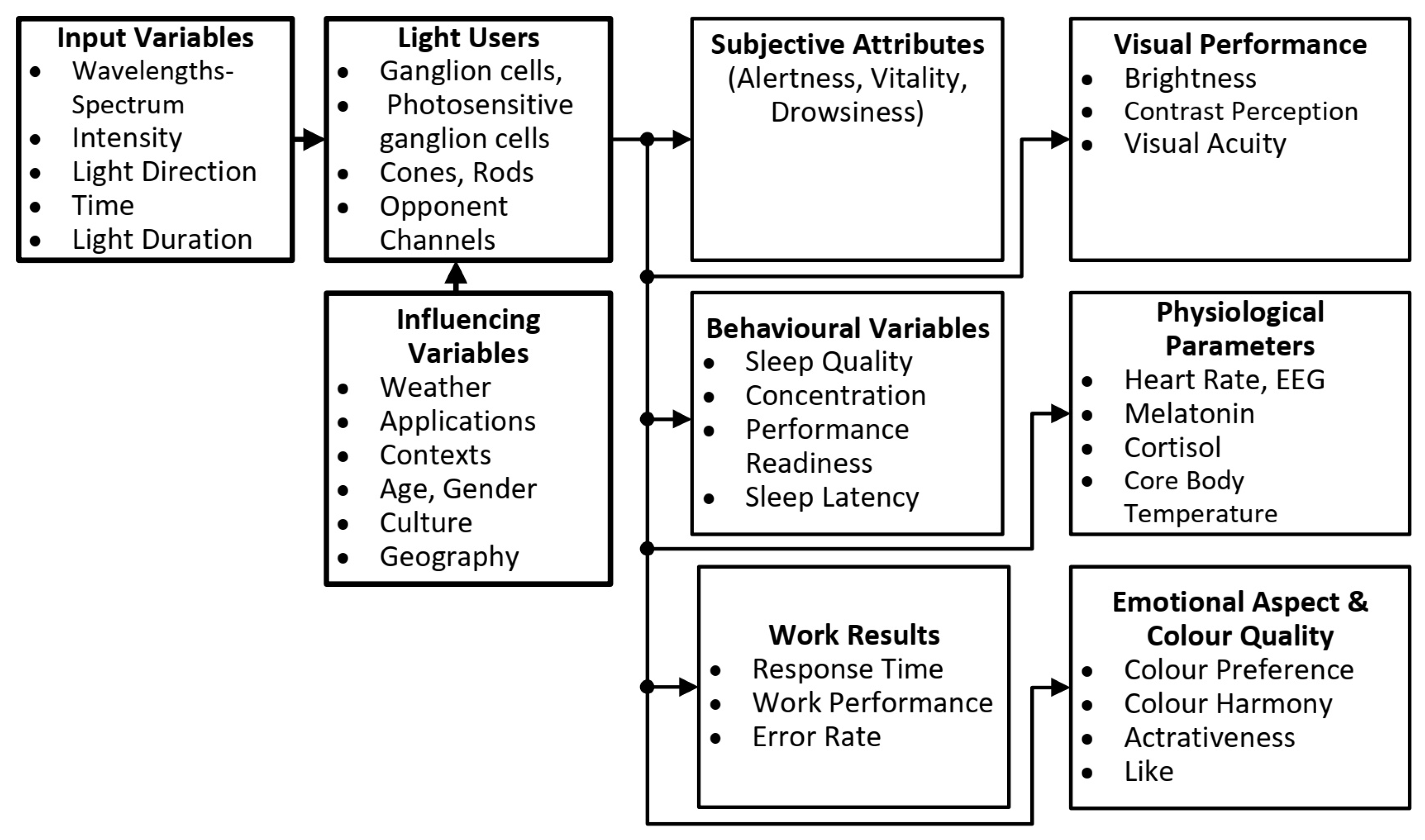
Figure 2.
Principle of a Smart Lighting concept with color sensors.
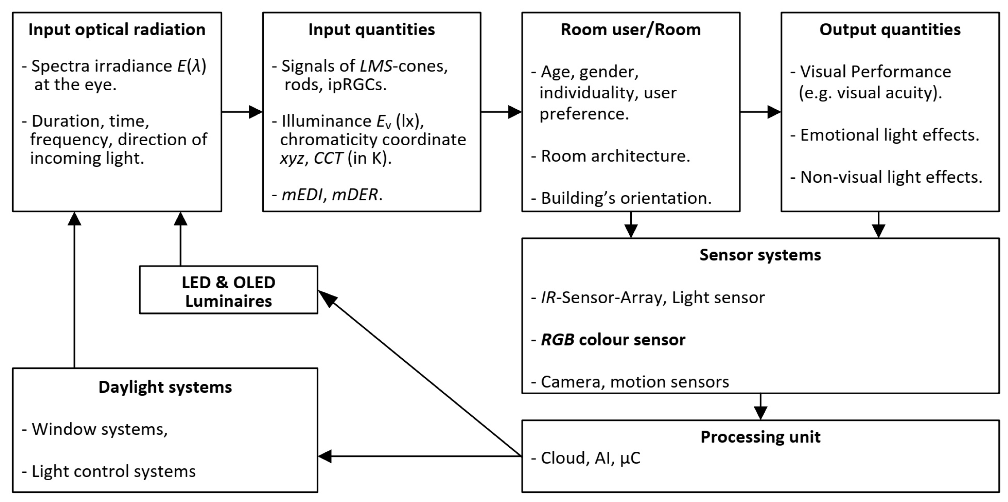
Figure 3.
System of relative photoreceptor sensitivities in CIE S 026/E:2018 [1].
Figure 3.
System of relative photoreceptor sensitivities in CIE S 026/E:2018 [1].
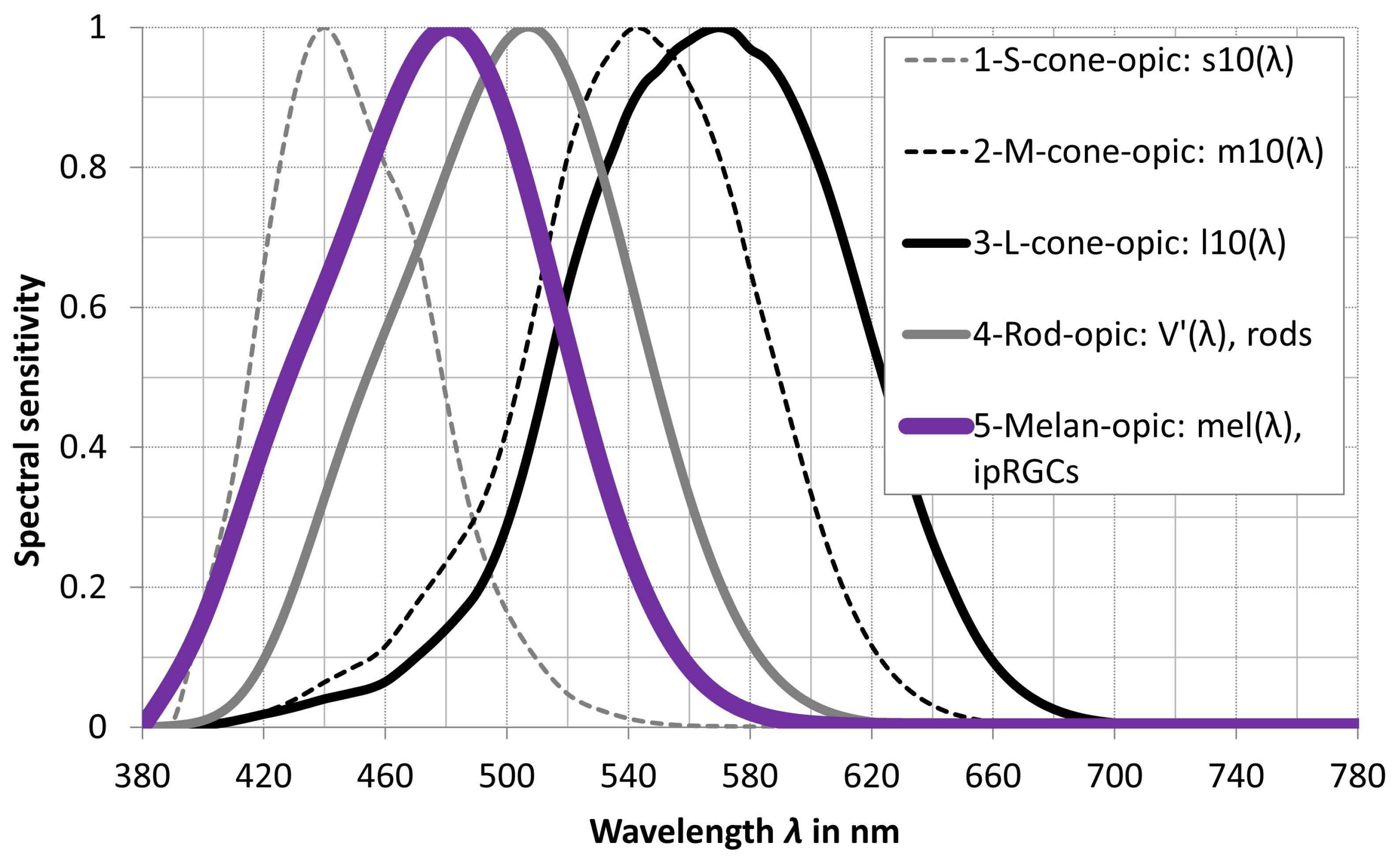
Figure 4.
4 Examples of color sensors - From left to right the color sensor chips MTCS-CDCAF, MRGBiCS and S11059 are shown. (Image Source: TU Darmstadt).
Figure 4.
4 Examples of color sensors - From left to right the color sensor chips MTCS-CDCAF, MRGBiCS and S11059 are shown. (Image Source: TU Darmstadt).
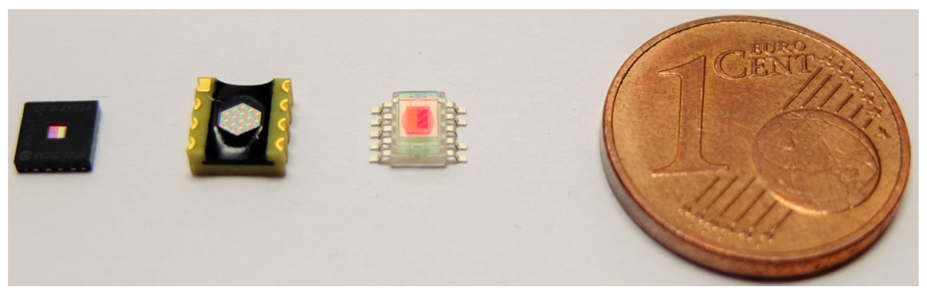
Figure 5.
Schematic arrangement for measuring the spectral sensitivity of sensors.
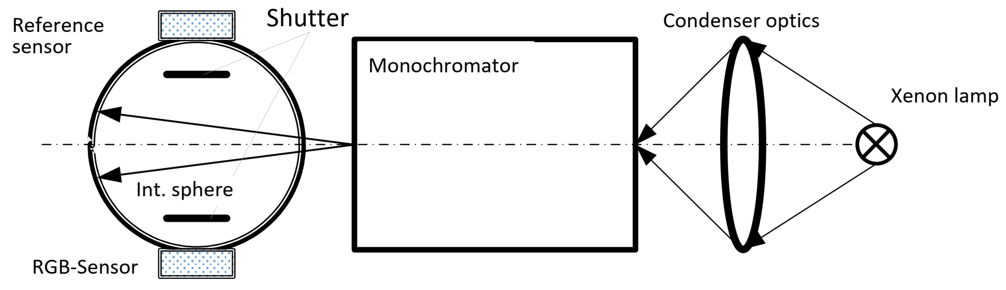
Figure 6.
Examples of the spectral sensitivity curves of some color sensors.
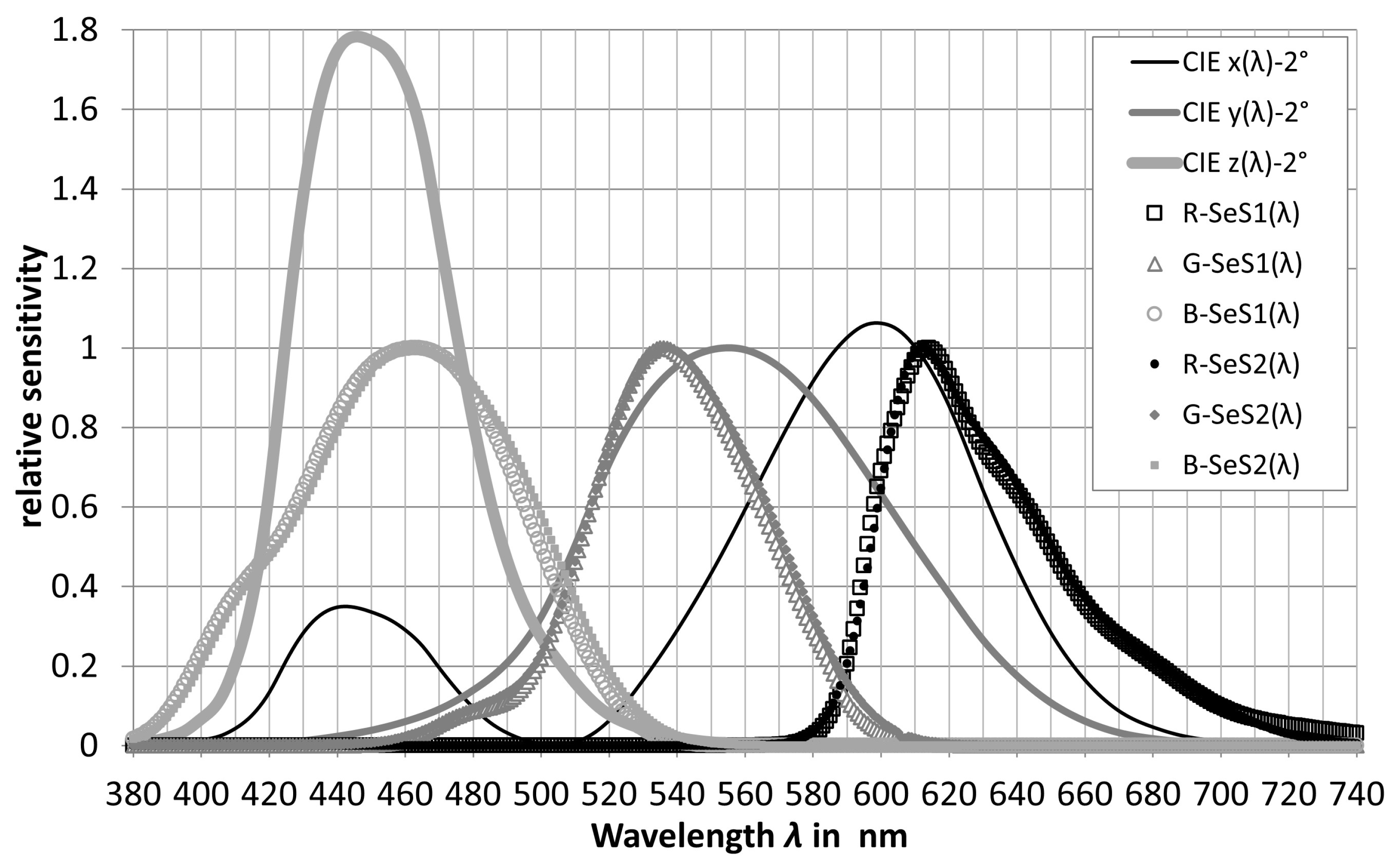
Figure 7.
Spectral sensitivity curves of another color sensor type.
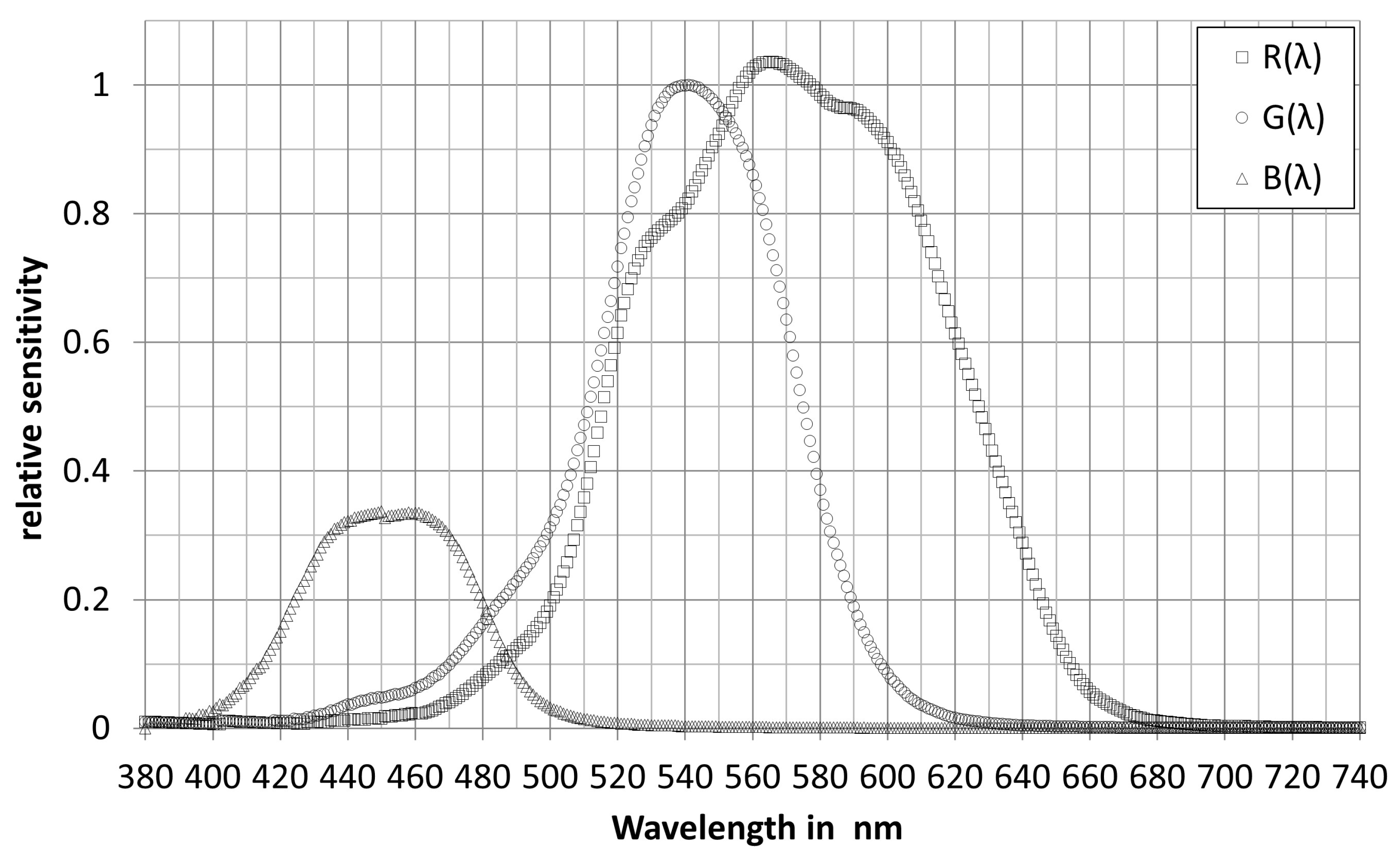
Figure 8.
Flowchart of the optimization of a transformation matrix from to based on the chromaticity difference [25].
Figure 8.
Flowchart of the optimization of a transformation matrix from to based on the chromaticity difference [25].
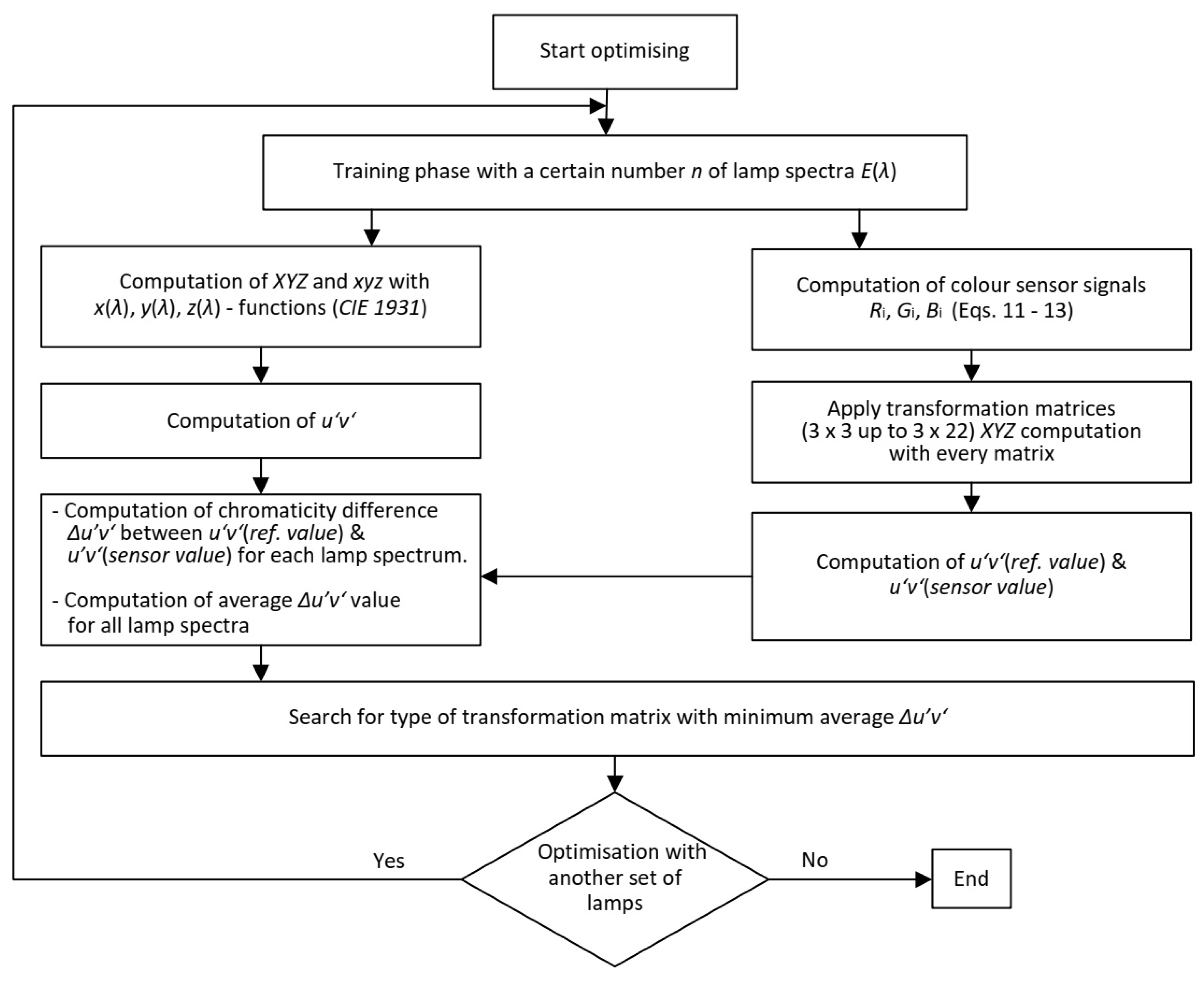
Figure 9.
Spectra of the lamp types for matrix optimization.
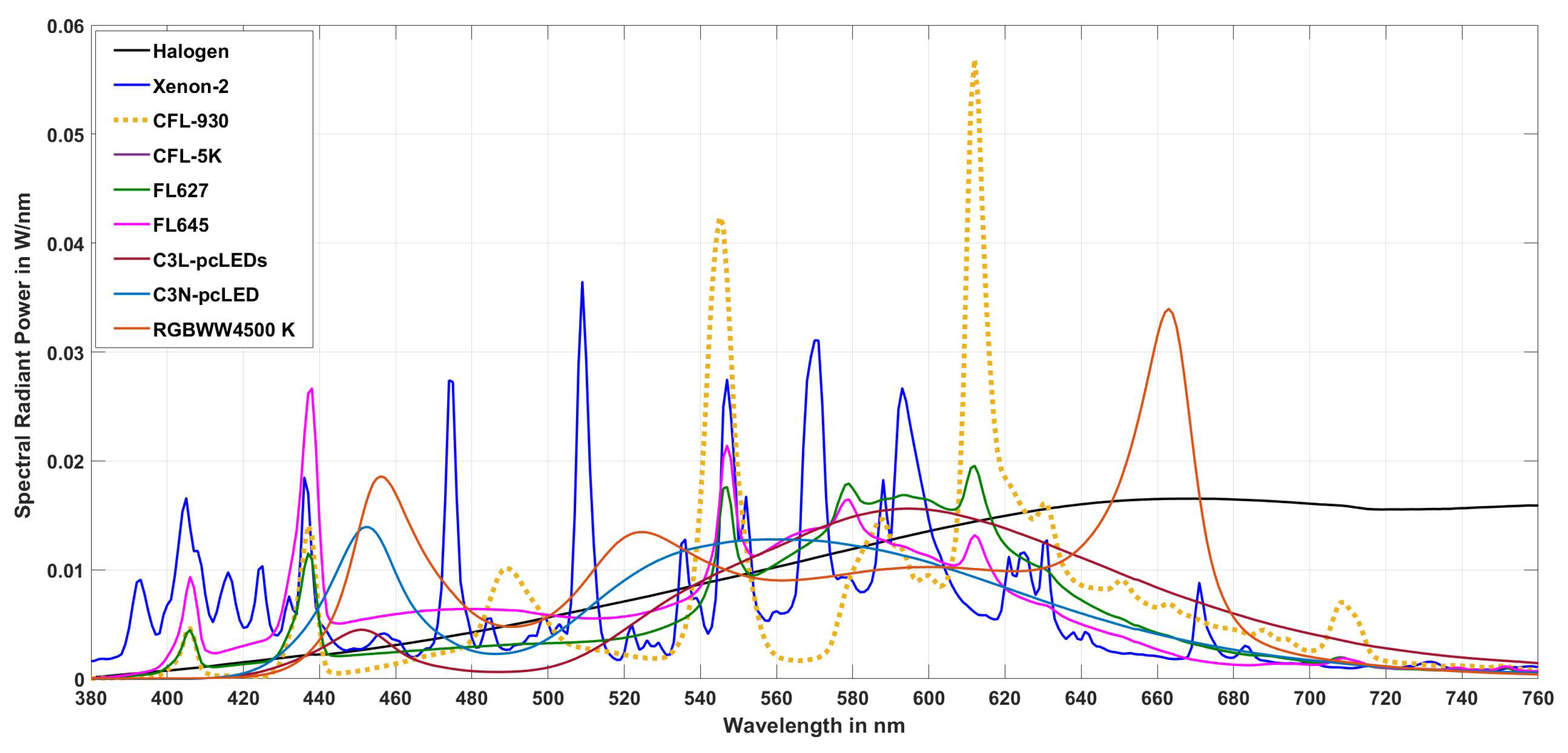
Figure 10.
Lamp spectra of 13 light source types for the validation of the 3 x 3 matrix in Table 7.
Figure 10.
Lamp spectra of 13 light source types for the validation of the 3 x 3 matrix in Table 7.
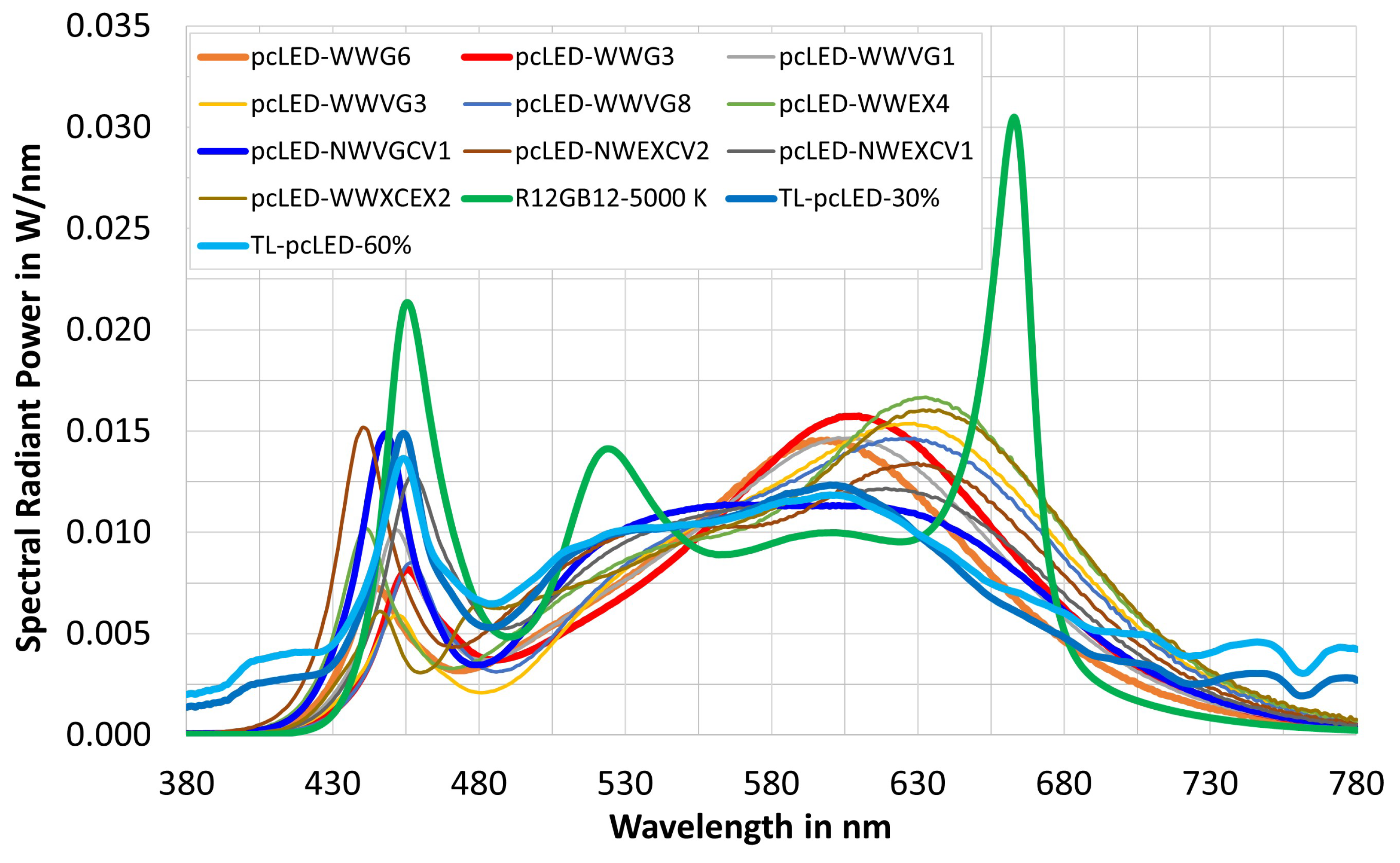
Figure 11.
Some daylight spectra on a sunny day in Darmstadt, Germany (on August 19th, 2020).
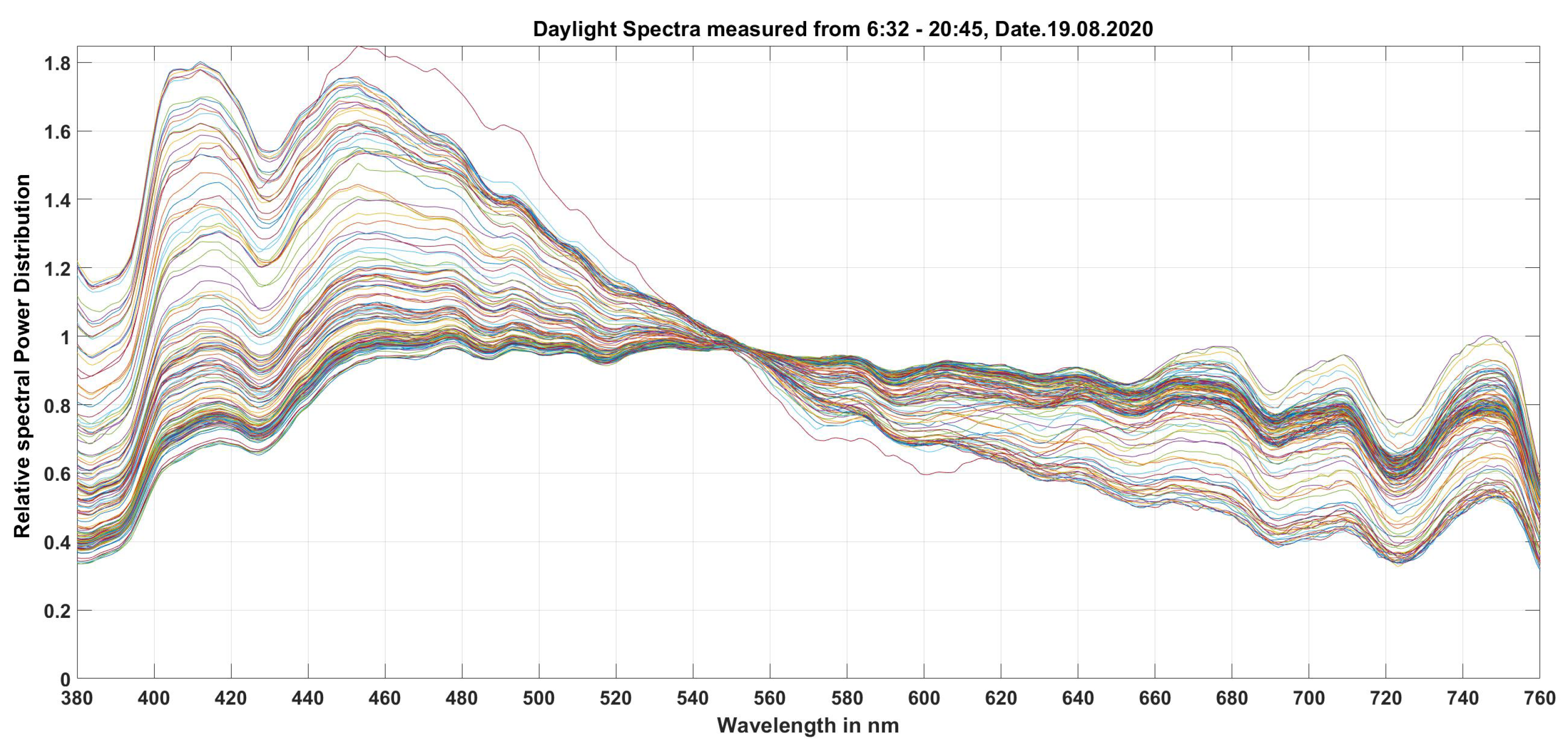
Figure 12.
Spectra of 884 measured light source spectra.
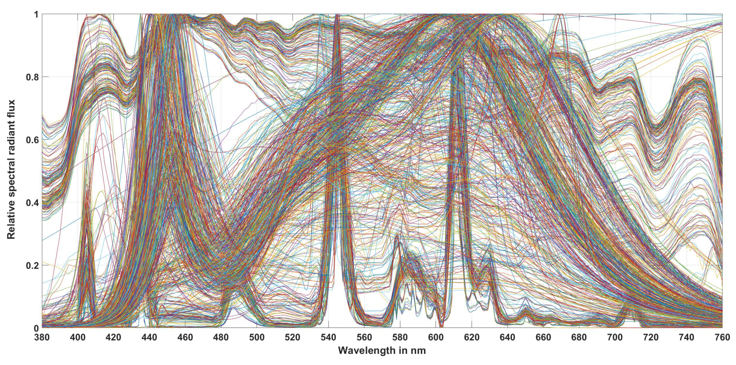
Figure 13.
Spectra of 185 phases of daylight, mixed with white LEDs in 9 mixture ratios from 10% until 90%.
Figure 13.
Spectra of 185 phases of daylight, mixed with white LEDs in 9 mixture ratios from 10% until 90%.
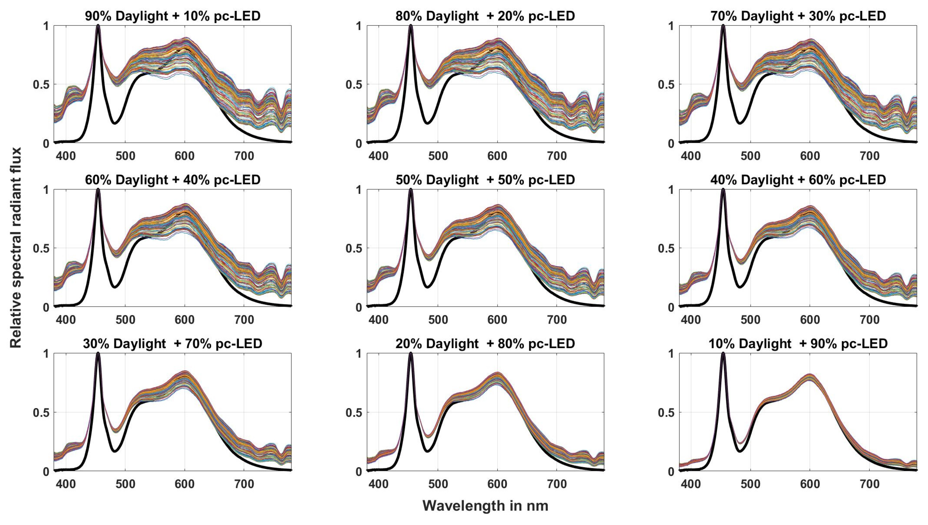
Figure 14.
Correlation between (ordinate) and the chromaticity coordinate z (abscissa).
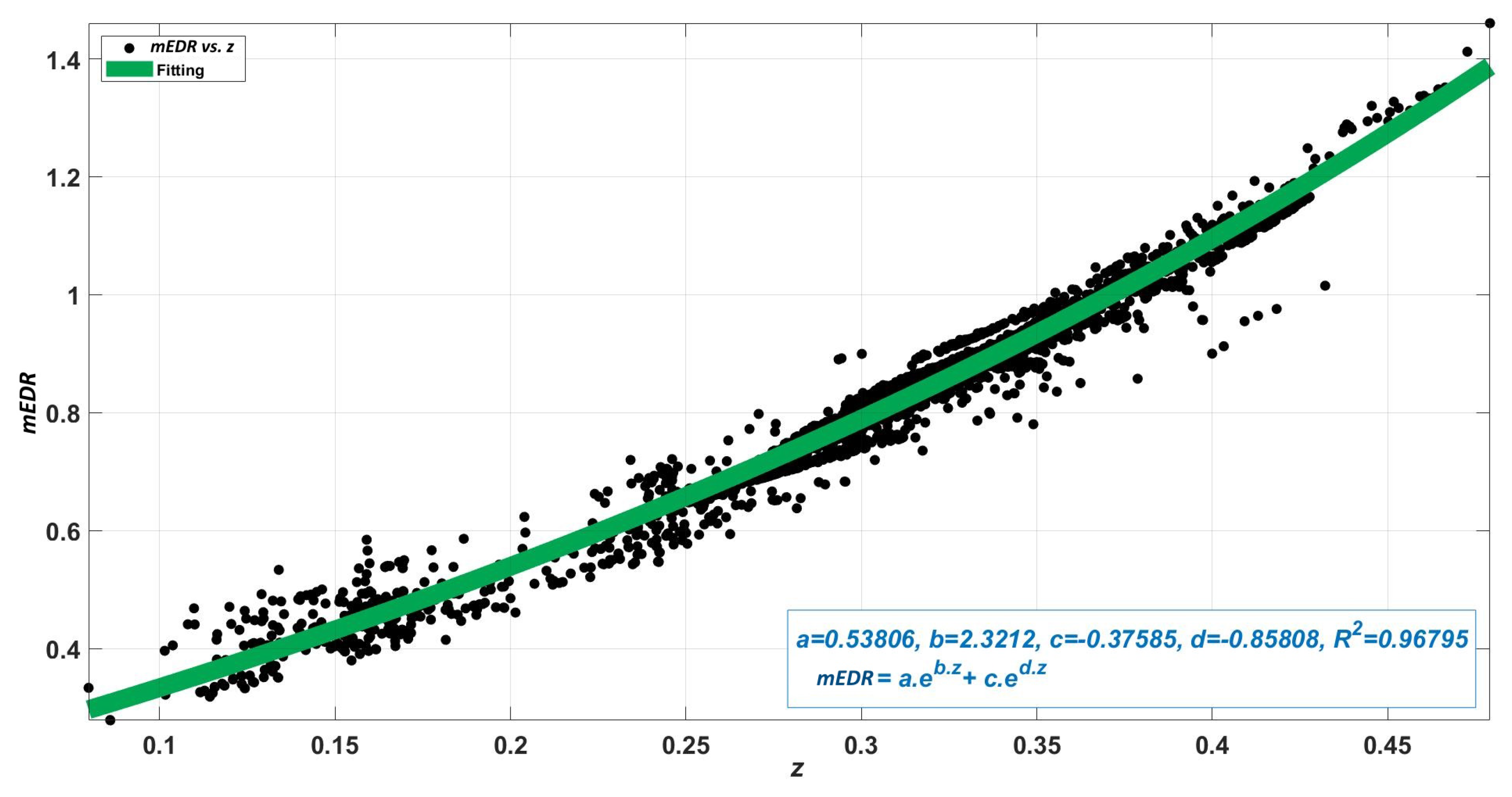
Figure 15.
Comparison of the 4214 values on the ordinate, calculated from the spectra themselves (denoted as ), with the 4214 values calculated using Equation 25. , the linear constants , compared to the ideal constants 1 and 0 and the 97% confidence interval of 0.067802 shows a good quality.
Figure 15.
Comparison of the 4214 values on the ordinate, calculated from the spectra themselves (denoted as ), with the 4214 values calculated using Equation 25. , the linear constants , compared to the ideal constants 1 and 0 and the 97% confidence interval of 0.067802 shows a good quality.
| No. | Parameter | Preferred values |
|---|---|---|
| 1 | Horizontal illuminance in lux [12,13,14] |
Greater than 850 lx; Recommended range: 1300 lx – 1500 lx |
| 2 | Correlated color temperature in K [15,16] | 4000 K - 5000 K |
| 3 | Color rendering index [10] | > 80 |
| 4 | Indirect to total illuminance ratio [11,17] | > 0.6 - 0.8 |
Table 2.
-opic quantities in CIE S 026/E:2018 [1]
Table 2.
-opic quantities in CIE S 026/E:2018 [1]
| -opic quantities | ||
|---|---|---|
| Parameter | Equation | Equation No. |
| -opic-radian flux | like (3.1) Page 4 [1] | |
| -opic-radiance | like (3.5) Page 4 [1] | |
| -opic-irradiance | like (3.6) Page 5 [1] | |
Table 3.
Melanopic equivalent D65 quantities of CIE S 026/E:2018 [1]
Table 3.
Melanopic equivalent D65 quantities of CIE S 026/E:2018 [1]
| -opic quantities | ||
|---|---|---|
| Parameter | Equation | Equation No. |
|
Melanopic Equivalent Daylight (D65) Illuminance (mEDI) in lx |
like (3.9) Page 6 [1] with =mel. |
|
|
Melanopic daylight (D65) efficacy ratio () |
↓ | |
| ↓ | ||
| like (3.10) Page 7 [1] with =mel. |
||
|
(*) Note: For the parameter (indices x, y according to the corresponding definitions), see Equation 4 and Euation 5 when α = mel. and apply Equation 15 when the calculated parameter is the mel-opic irradiance. | ||
Table 4.
Different matrix types for color sensing according to [26]
Table 4.
Different matrix types for color sensing according to [26]
| Nr. | Size | Content |
|---|---|---|
| 1 | 3 x 3 | [R G B] |
| 2 | 3 x 5 | [R G B 1] |
| 3 | 3 x 7 | [R G B RG RB GB 1] |
| 4 | 3 x 8 | [R G B RG RB GB 1] |
| 5 | 3 x 10 | [R G B RG RB GB 1] |
| 6 | 3 x 11 | [R G B RG RB GB 1] |
| 8 | 3 x 14 | [R G B RG RB GB 1] |
| 9 | 3 x 16 | [R G B RG RB GB G B R ] |
| 10 | 3 x 17 | [R G B RG RB GB G B R 1] |
| 11 | 3 x 19 | [R G B RG RB GB G B R B R G ] |
| 12 | 3 x 20 | [R G B RG RB GB G B R B R G 1] |
| 13 | 3 x 22 | [R G B RG RB GB G B R B R G GB RB RG] |
Table 5.
Properties of the lamp types for matrix optimization
| Lamp type | Tungsten halogen | Xenon-2 | CFL 3000K | CFL 5000 K | FL 627 | FL 645 | LED C3L | LED c3N | LED RGBWW4500 |
|---|---|---|---|---|---|---|---|---|---|
| CCT (in K) | 2762 | 4100 | 2640 | 4423 | 2785 | 4423 | 2640 | 4580 | 4500 |
| Duv () | 3 | 7.2 | 0.61 | 2.2 | 1.8 | 2.2 | 6.3 | 1.3 | -1.0 |
| Ev (in lx) | 750 | 750 | 750 | 750 | 750 | 750 | 750 | 750 | 750 |
| CIE R9 | 85 | -86 | 48 | -60 | -72 | -60 | -28 | -39 | 36 |
| CIE Ra | 97 | 67 | 90 | 68 | 64 | 68 | 67 | 69 | 90 |
Table 6.
Chromaticity difference for different matrix types for the lamp types of the training set
| Name | Xenon-2 | CFL-930 | CFL-5K | FL627 | FL645 | C3L-pcLEDs | C3N-pcLED | RGBWW4500 K | Max |
|---|---|---|---|---|---|---|---|---|---|
| 7.4 | 7.7 | 1.5 | 4.5 | 1.5 | 0.42 | 2.7 | 8.3 | 8.3 | |
| 4.8 | 48 | 12 | 41 | 12 | 51 | 16 | 16 | 51 | |
| 8.5 | 5.3 | 1.6 | 7.0 | 20 | 6.4 | 20 | |||
| 6.9 | 32 | 11 | 40 | 11 | 48 | 7.0 | 16 | 48 | |
| 2.9 | 4.5 | 0.92 | 12 | 3.8 | 12 | ||||
| 7.9 | 2.2 | 37 | 2.2 | 42 | 12 | 8.1 | 42 | ||
| 7.1 | 10 | 7.8 | 1.7 | 6.7 | 10 | ||||
| 8.4 | 5.7 | 3.0 | 2.5 | 1.9 | 10 | 10 | |||
| 8.4 | 5.7 | 3.0 | 2.5 | 1.9 | 10 | 10 | |||
| 7.2 | 9.1 | 4.3 | 5.7 | 7.5 | 9.1 | ||||
| 7.2 | 9.1 | 4.3 | 5.7 | 7.5 | 9.1 | ||||
| 6.6 | 8.9 | 2.2 | 3.2 | 7.2 | 8.9 |
Table 7.
Optimum matrix (3 x 3) for the transformation to as well as the formula for the calculation of the illuminance Ev from the signals
Table 7.
Optimum matrix (3 x 3) for the transformation to as well as the formula for the calculation of the illuminance Ev from the signals
| (lx) from R, G, B | |
|---|---|
| ; | |
| Matrix 3 x 3 in case of the 9 light sources of training set |
Table 8.
Verification of optimal matrix (3 x 3) in Table 7 with 13 LEDs plus mixed daylight spectra
Table 8.
Verification of optimal matrix (3 x 3) in Table 7 with 13 LEDs plus mixed daylight spectra
| Name | pcLED-WWG6 | pcLED-WWG3 | pcLED-WWVG1 | pcLED-WWVG3 | pcLED-WWVG8 | pcLED-WWEX4 | pcLED-NWVG1 | pcLED-NWEXCV2 | pcLED-CWVG1 | pcLED-CWEX2 | R12GB12-5000 K | TL-pcLED-30% | TL-pcLED-60% |
|---|---|---|---|---|---|---|---|---|---|---|---|---|---|
| (K) | 3134 | 2801 | 3105 | 2782 | 2998 | 2969 | 4614 | 3942 | 5112 | 5059 | 5001 | 4391 | 4571 |
| 80.27 | 84.06 | 85.63 | 88.10 | 90.56 | 94.41 | 90.91 | 93.09 | 90.06 | 95.99 | 89.73 | 89.85 | 92.48 | |
| x | 0.4285 | 0.4434 | 0.4217 | 0.4557 | 0.4352 | 0.4252 | 0.3569 | 0.3764 | 0.3424 | 0.3439 | 0.3449 | 0.3644 | 0.3581 |
| y | 0.4025 | 0.3929 | 0.3841 | 0.4135 | 0.4003 | 0.3765 | 0.3608 | 0.3550 | 0.3537 | 0.3557 | 0.3495 | 0.3650 | 0.3605 |
| (lx) | 750 | 750 | 750 | 750 | 750 | 750 | 750 | 750 | 750 | 750 | 750 | 750 | 750 |
| 750.35 | 752.29 | 752.54 | 750.90 | 751.14 | 754.17 | 751.40 | 754.79 | 751.31 | 750.01 | 747.60 | 751.94 | 751.91 | |
| 0.4285 | 0.4434 | 0.4217 | 0.4557 | 0.4352 | 0.4252 | 0.3546 | 0.3779 | 0.3361 | 0.3368 | 0.3319 | 0.3665 | 0.3572 | |
| 0.4025 | 0.3929 | 0.3841 | 0.4135 | 0.4003 | 0.3765 | 0.3643 | 0.3698 | 0.3545 | 0.3571 | 0.3529 | 0.3696 | 0.3640 | |
| 3.15 | 8.76 | 4.5 | 5.32 | 10.1 | 2.42 | 2.51 | |||||||
| in % | 0.05 | 0.31 | 0.34 | 0.12 | 0.15 | 0.56 | 0.19 | 0.64 | 0.17 | 0.00 | -0.32 | 0.26 | 0.25 |
Table 9.
Optimal matrix (3 x 3) for transforming to and formula for calculating illuminance from signals in case of pure daylight.
Table 9.
Optimal matrix (3 x 3) for transforming to and formula for calculating illuminance from signals in case of pure daylight.
| (lx) from R, G, B | |
|---|---|
| ; | |
| Matrix 3 x 3 in the case of the 9 light sources of the training set |
Table 10.
Verification of the 3 x 3 matrix for daylight spectra (trained on a sunny day, verified on a rainy day)
Table 10.
Verification of the 3 x 3 matrix for daylight spectra (trained on a sunny day, verified on a rainy day)
| Sampling Time | 07:27:17 | 10:03:31 | 11:06:01 | 12:03:19 | 13:05:50 | 14:07:40 | 15:10:10 | 16:12:41 | 19:14:58 |
|---|---|---|---|---|---|---|---|---|---|
| in K | 12464 | 8033 | 6313 | 5651 | 5914 | 5853 | 5470 | 8174 | 16066 |
| in lx | 401 | 9397 | 23940 | 58212 | 39463 | 43150 | 71006 | 15058 | 461 |
| 0.2652 | 0.2942 | 0.3163 | 0.3291 | 0.3236 | 0.3248 | 0.3332 | 0.2919 | 0.2568 | |
| 0.2831 | 0.3066 | 0.3293 | 0.3413 | 0.3364 | 0.3376 | 0.3449 | 0.3081 | 0.2705 | |
| in lx | 400.60 | 9403.02 | 23944.07 | 58205.57 | 39465.20 | 43149.59 | 70987.13 | 15070.62 4 | 60.41 |
| 4.75 | 1.74 | 1.20 | 1.82 | 1.96 | 0.596 | 4.03 | 8.57 |
Table 11.
Measured and simulated spectra (4214 in total)
| No. | Type of light sources and their parameter ranges = 2201 – 17815 K; -1.467 < < 1.529 0.0797 < z < 0.4792; 80 < < 100; 0.2784 < < 1.46 |
|---|---|
| 1. | Conventional incandescent lamps + filtered incandescent lamps |
| 2. | Fluorescent tubes + Compact fluorescent lamps |
| 3. | LED lamps + LED luminaires |
| 4. | Daylight (CIE-model + measurements) |
| 5. | Mixtures (DL+LED) - [ mixture ratio = 10%-90% ] |
| 6. | Mixtures (DL+FL) - [ mixture ratio = 10%-90% ] |
Table 12.
Parameter a, b, c and d for the fit function in Equation 25 and the correlation coefficient
Table 12.
Parameter a, b, c and d for the fit function in Equation 25 and the correlation coefficient
| Parameter | a | b | c | d | |
|---|---|---|---|---|---|
| Value | 0.53806 | 2.3212 | -0.37585 | -0.85808 | 0.968 |
Disclaimer/Publisher’s Note: The statements, opinions and data contained in all publications are solely those of the individual author(s) and contributor(s) and not of MDPI and/or the editor(s). MDPI and/or the editor(s) disclaim responsibility for any injury to people or property resulting from any ideas, methods, instructions or products referred to in the content. |
© 2023 by the authors. Licensee MDPI, Basel, Switzerland. This article is an open access article distributed under the terms and conditions of the Creative Commons Attribution (CC BY) license (https://creativecommons.org/licenses/by/4.0/).
Copyright: This open access article is published under a Creative Commons CC BY 4.0 license, which permit the free download, distribution, and reuse, provided that the author and preprint are cited in any reuse.


