Submitted:
05 April 2023
Posted:
06 April 2023
You are already at the latest version
Abstract
Deep learning has been applied in many areas that have had a significant impact on applications that improves real-life challenges. The success of deep learning in a wide range of areas is due in part to the use of activation functions, which are particularly effective at solving non-linear problems. Activation functions are a key focus for researchers in artificial intelligence who aim to improve the performance of neural networks. This article provides a comprehensive explanation and comparison of different activation functions, with a focus on the arc tangent and its variations specifically. The paper presents experimental results that show that variations of the arc tangent using irrational numbers such as pi, the golden ratio, and Euler’s number, as well as a self-arctan function, produce promising results. Since we experimented with promising activation functions on two different problems, and datasets, we reached a result that different irrationals work well for different problems. In other words, arctan ϕ gives the best results mostly for multiclass classification and arctan e gives the best results for time series prediction problems. The paper focuses on a multi-class classification problem applied to the Reuters Newswire dataset and a time-series prediction problem on Türkiye energy trade value to show the impacts of activation functions.
Keywords:
Deep neural networks
; Activation functions
; Multi-class classification
; Time-Series prediction
; Reuters data
; Energy trade value
1. Introduction
Deep learning is a powerful and versatile methodology that has a wide range of applications in various fields, such as healthcare [8], natural language processing applications [7], drug discovery [5], autonomous vehicles [6], finance [9], cyber security [2], and many others. It is a class of machine learning algorithms that go beyond traditional methods, such as multilayer neural networks with many hidden units, to learn complex predictive models [20]. When learning to approximate complex problems, activation functions play a crucial role by introducing nonlinearity, which is essential for many tasks. Some examples of activation functions include sigmoid, ReLU, and tanh, which have been widely used in deep learning due to their ability to model complex and nonlinear relationships between input and output data [19]. Overall, deep learning has become a promising approach for solving many real-world problems thanks to activation functions.
According to the modifications of the universal approximation theorem for neural networks, under certain conditions on the activation function, a single-hidden layer neural network can approximate any continuous function arbitrarily well [12,13,14,15,16]. This means that, given enough data and suitable network architecture, a neural network can learn to approximate complex functions and make accurate predictions for a wide range of tasks. However, the effectiveness and performance of a neural network can vary depending on the specific problem and the characteristics of the data, as well as the choice of the activation function [18]. For example, some activation functions may be more effective for certain tasks or data types, while others may perform better for other tasks or data. Therefore, selecting the appropriate activation function is an important aspect of neural network design and can significantly impact the accuracy and efficiency of the model. In our work, we experimented with time series prediction and multiclass classification problems to find out how activation functions range affects the training time and models’ success. Different ranges were obtained by dividing irrational numbers like pi, the golden ratio, and the Euler number, specifically applied to the arctan function. As a result of the experiments, we observed remarkable results.
2. Related Work
While developing more optimized algorithms, there are many researches focusing on activation functions. It is a common research problem that develops optimized models with the help of activation functions. There is a wide range of research that presents the efficiency of activation functions on different datasets and problems. Firstly, we proposed the arctan function’s variations with irrational numbers such as pi and the golden ratio and the self-arctan function applied to multiclass classification problem with Reuters news wire classification dataset [1]. Skoundrianos and Tzafestas (2004) [24] developed a sigmoidal activation function for modeling dynamic, discrete time systems. Efe (2008) [23] proposed activation functions which are sinc and cosc experimented on eight different datasets.
An activation function was developed by Liew et al. (2016) [22] which sets a boundary from the positive side of the ReLU applied on MNIST handwritten digit dataset. Sharma (2019) [21] proposed an activation function that is a combination of the sigmoid and ReLU (Rectified Linear Unit) applied to the ionosphere dataset which is a radar system dataset with continuous values. Misra et al. (2020) [17] proposed a non-monotonic self-regularized activation function which is a composition of tanh and softplus functions and a multiplication of input values. It experimented on CIFAR-10, ImageNet-1k, and MS-COCO Object Detection. The recent research made by Jin et al. (2022) [28] focuses on solving the Time-varying Sylvester equation using Zeroing Neural Network based on the Versatile Activation Function (VAF) variations which include exponential convergence characteristic and adjustable parameter. Another recent work proposed a function called Smish by Wang et al. (2022) [29]. It was experimented on the CIFAR-10 dataset with the EfficientNetB3 network, on the MNIST dataset with the EfficientNetB5 network, and on the SVHN dataset with the EfficientnetB7 network. Furthermore, Shui-Long et al. (2022) [25] developed an activation function, named as tanhLU which it uses the symmetry feature of tanh and the unbounded feature of ReLU. It experimented on seven different benchmark datasets which are MNIST, CASIA-webface, Penn Treebank Dataset (PTB), LFW, CIFAR-10, CIFAR-100, datasets and neural network architectures like Fully Connected Neural Network (FCNN), Long Short-Term Memory (LSTM), and Convolutional Neural Network (CNN).
In this article, we present a novel approach that focuses on using variations of the arctan function, specifically those that are based on the combination of input and tanh function and the irrational numbers pi, the golden ratio, and the Euler number. Our experiments demonstrate that this approach can significantly improve training time compared to the topic classification problem. Furthermore, experiments show that promised activation functions produced better and closer results for both problems. Overall, our results indicate that this new approach has great potential for improving the performance of machine learning models.
3. Activation Functions
Activation functions are used in artificial neural networks to determine whether a neuron should be activated or not. These functions take the input from the previous layer of the neural network, sum the weighted input, and then transform it into an output that will be passed to the next layer of the network. Activation functions are often referred to as transfer functions in deep learning because they help to transfer the input to the next layer of the network [26]. In other words, they act as a mathematical gate between the input and the current neuron, allowing the network to decide which information is relevant and should be passed on to the next layer. Overall, the activation function plays a crucial role in the process of deep learning, as it determines which information is important and should be used to make predictions or decisions.
The activation function is a key component of a neural network. Its primary role is to introduce non-linearity into the network [19], which is necessary for the network to be able to learn complex tasks. Without non-linearity, the network would only be able to perform linear transformations and would not be able to tackle more complicated problems. Non-linearity allows the network to make decisions based on conditional relationships, rather than just relying on a linear function to solve all problems. In addition to adding non-linearity, the activation function must also be differentiable [11]. This property is important because it allows the network to use gradient-based optimization algorithms, which are essential for training the network. Differentiability also enables the network to learn by making small adjustments to the weights and biases of the network, rather than having to start from scratch every time. Overall, the activation function plays a critical role in enabling neural networks to learn and make decisions in a way that is flexible and adaptable to different types of tasks. It allows the network to process and analyze complex data, and to find solutions that are numerically close to the original function, even if the exact function is unknown.
There are three types of activation functions used in Deep Neural Networks (DNN): binary step functions [4], linear activation functions, and nonlinear activation functions. First of all, binary step functions are not useful for solving deep learning problems because they only output a single value (either 0 or 1). They also have a zero gradient, which can cause problems when using backpropagation to update the weights in the network. The second is linear activation functions. They are not effective at approximating complex, nonlinear relationships. This is because their derivative is constant, meaning that they will not learn any new information during training. Lastly, nonlinear activation functions, on the other hand, are able to approximate a wide range of complex, nonlinear relationships and can be used for multiclass classification and regression tasks. Some examples of nonlinear activation functions include sigmoid, tanh, and ReLU. Each function has its own pros and cons according to the problem they consider. In this work, the purpose is to give a comparison of the arctan function and its variations with the others showing and explaining their effectiveness while playing with arctan’s range. In the following sections, activation functions and experiments are explained in detail.
3.1. Rectified Linear Unit (ReLU)
Rectified Linear Unit (ReLU) [4] is a widely used activation function in deep learning models. It is defined as in Table 1. In other words, the output of the ReLU function is the maximum of 0, and the input value x. If x is greater than 0, the output is equal to x. If x is less than or equal to 0, the output is 0. The ReLU function has a simple, piecewise linear form and has several desirable properties for use in neural networks. It and its gradient, see Table 1, are computationally efficient because they do not require any expensive operations such as exponentiation or logarithms, and ReLU has a fast convergence rate during training. It also does not saturate for large input values, which can lead to vanishing gradients and slow training. ReLU is often used as an activation function in hidden layers of deep neural networks and has been found to work well in a wide range of applications. However, it can sometimes produce outputs that are "dead" (i.e., the output is always 0) if the network is not properly initialized or trained, or if the input data is not properly normalized. Variations like Leaky ReLU, Exponential Linear Unit (ELU), Scaled Exponential Linear Unit (SELU), parametric ReLU, etc. can be a solution to the vanishing gradient problem depending on the problem.
3.2. Leaky ReLU
Leaky ReLU [4] is a variant of the standard ReLU activation function that has a small, non-zero slope for negative input values. This helps address the issue of "dying ReLUs," which is a problem that can occur when using the standard ReLU function in neural networks. In other words, neurons that have negative weights will be updated unlike ReLU, and it allows a small, non-zero gradient for negative input values, see Table 1. For positive input values, leaky ReLU behaves like the standard ReLU function, mapping the input to itself. For negative input values, leaky ReLU maps the input to a small, non-zero value determined by the constant , see Table 1. Leaky ReLU has been shown to improve the performance of neural networks in certain tasks and is often used as an alternative to the standard ReLU function. However, it is important to carefully tune the value of the constant a to ensure that the model is not overfitting the training data.
3.3. Sigmoid
The sigmoid function [4] is a mathematical function that maps values from an input space to a range between 0 and 1. It is often used as an activation function in neural networks, particularly in binary classification tasks, where the output of the network is interpreted as a probability. The sigmoid function is defined as in Table 1, where x is the input value and e is the base of the natural logarithm. It has an S-shaped curve, with an output of 0.5 when the input is 0. One of the main advantages of the sigmoid function is that its output is always bounded between 0 and 1, which makes it well-suited for modeling probabilities. However, the sigmoid function can also suffer from some limitations. For example, the output of the sigmoid function is not zero-centered, which can make it difficult to model certain types of relationships. In addition, the derivative of the sigmoid function (see Table 1) becomes very small for large positive or negative input values, which can make it difficult to train deep neural networks using the sigmoid function. Despite these limitations, the sigmoid function remains a popular choice for activation functions in neural networks and is often used in conjunction with other activation functions to achieve good performance on a wide range of tasks.
3.4. Hyperbolic Tangent (tanh)
The hyperbolic tangent (tanh) function [4], shown in Table 1, is a mathematical function that maps values from an input space to a range between -1 and 1. It is often used as an activation function in neural networks, particularly in tasks where the output of the network needs to be interpreted as a continuous value. One of the main advantages of the tanh function is that its output is zero-centered, which makes it well-suited for modeling certain types of relationships. In addition, the derivative of the tanh function, see Table 1, is relatively large for most input values, which can make it easier to train deep neural networks using the tanh function. However, the tanh function can also suffer from some limitations. For example, the output of the tanh function is not bounded, which can make it difficult to model probabilities. In addition, the tanh function can saturate for very large positive or negative input values, which can slow down the training process.
3.5. Swish
Swish [4] is a modified sigmoid function introduced by Google researchers, see Table 1. It has no upper limit but a lower limit. It is smooth and continuously differentiable, which can make it easier to optimize the model using gradient-based methods, see Table 1. Additionally, negative values are captured and large negative values are disabled from the pattern. It provides sparsity. However, it can saturate and produce very small gradients when the input is very large or very small, which can slow down the training process. It provides sparsity.
Figure 1.
Activation functions and derivatives

3.6. Arctan
The arctan function [3], also known as the inverse tangent function, is a mathematical function that takes a value as input and returns the angle in radians that has a tangent equal to that value, see Table 1. It is also S-shaped function like sigmoid; however arctan’s range is wider, i.e., . Additionally, a convex error surface is provided by its monotonicity (faster backpropagation).
4. Promised Activation Functions
Activation functions are powerful gates for solving a problem with deep learning models. In this section, we provide promised activation functions in detail. Specifically, the arctangent function’s variations are explained. These functions use irrational numbers like the golden ratio, the Euler number, and pi. Also, we defined a self-arctan function that uses the input directly in computations. Promised activation functions are designed to show the effect of functions’ range manipulation with irrational numbers and the power of symmetry. Variations of arctan functions and their derivatives can be observed in Figure 2 and Figure 2 respectively.
4.1. Arctan
Arctan is a variation of arctan where arctan is divided with , see Table 1. With purpose is to give a narrower range to arctan using the irrationality of . So, range become . Other properties are the same as the arctan function.
4.2. Arctan Golden Ratio ()
Arctan with golden ratio is a variation of arctan where arctan is divided with , see Table 1. In this activation function, a narrower range is the purpose according to arctan using the irrationality of the golden ratio. Thus, range become . Other properties are the same as the arctan function.
4.3. Arctan Euler
Arctan with Euler number is another variation that we used to experiment with how the Euler number affects the range of arctan to train a neural network architecture, see Table 1 for details of it. Dividing arctan function with Euler number stacks the range between . Other properties are the same as the arctan function.
4.4. Self Arctan
Using the input itself with arctan is used to obtain symmetry according to the y-axis, see Table 1. Thus, negative and positive outputs will be treated similarly. Also, negative weights will not be lost like ReLU. Furthermore, it is smooth, i.e., differentiable at every point. It acts like a second-degree polynomial around zero.
Figure 2.
Graphs of functions and derivatives of arctan and its variations. Figure 2 shows the functions graphs and Figure 2 shows the functions derivatives. These graphs enable us to compare the ranges of variations.
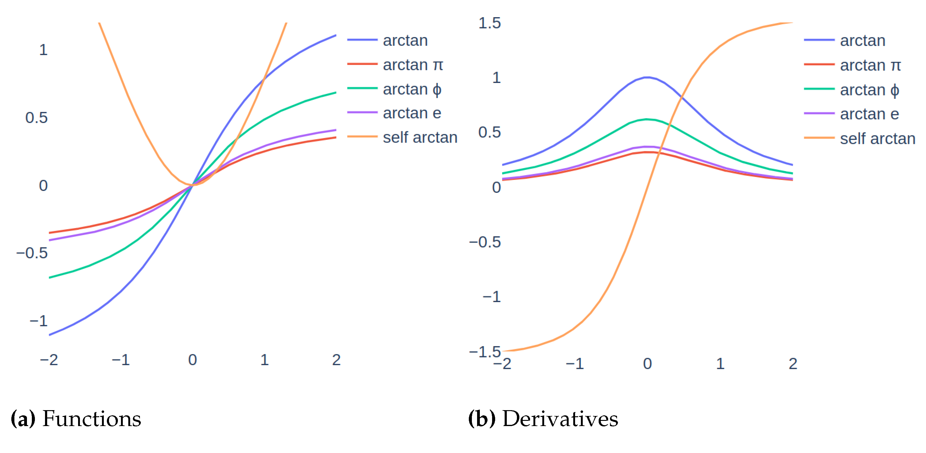

Table 1.
Activation functions
| Function name | Function | Derivative | Range |
|---|---|---|---|
| ReLU | |||
| leaky ReLU | |||
| sigmoid | |||
| tanh | |||
| swish | |||
| arctan | |||
| arctan | |||
| arctan | |||
| arctan e | |||
| self arctan |
5. Experiment
As we mentioned in the previous sections, deep learning can be used for solving different problems. While training the models, the effectiveness of activation functions can be different according to the problem and the data. In order to see the impacts of promised activation functions, we experimented with two different problems which are topic classification and time series prediction. While solving the problem we implemented two different models for each problem. The details are explained in the following sections.
5.1. Topic Classification
Topic classification is a widely used problem in machine learning. Reuters news wire classification dataset was used in the experiments. It is a multiclass dataset with 46 different topics. It contains 11.228 news-wires from Reuters. The dataset was generated by preprocessing and parsing the classic Reuters-21578 dataset. Furthermore, it is an unbalanced dataset, i.e., the class example numbers are not close. For example, there are approximately 4000 samples for one label and there are approximately 20 samples for more than one label.
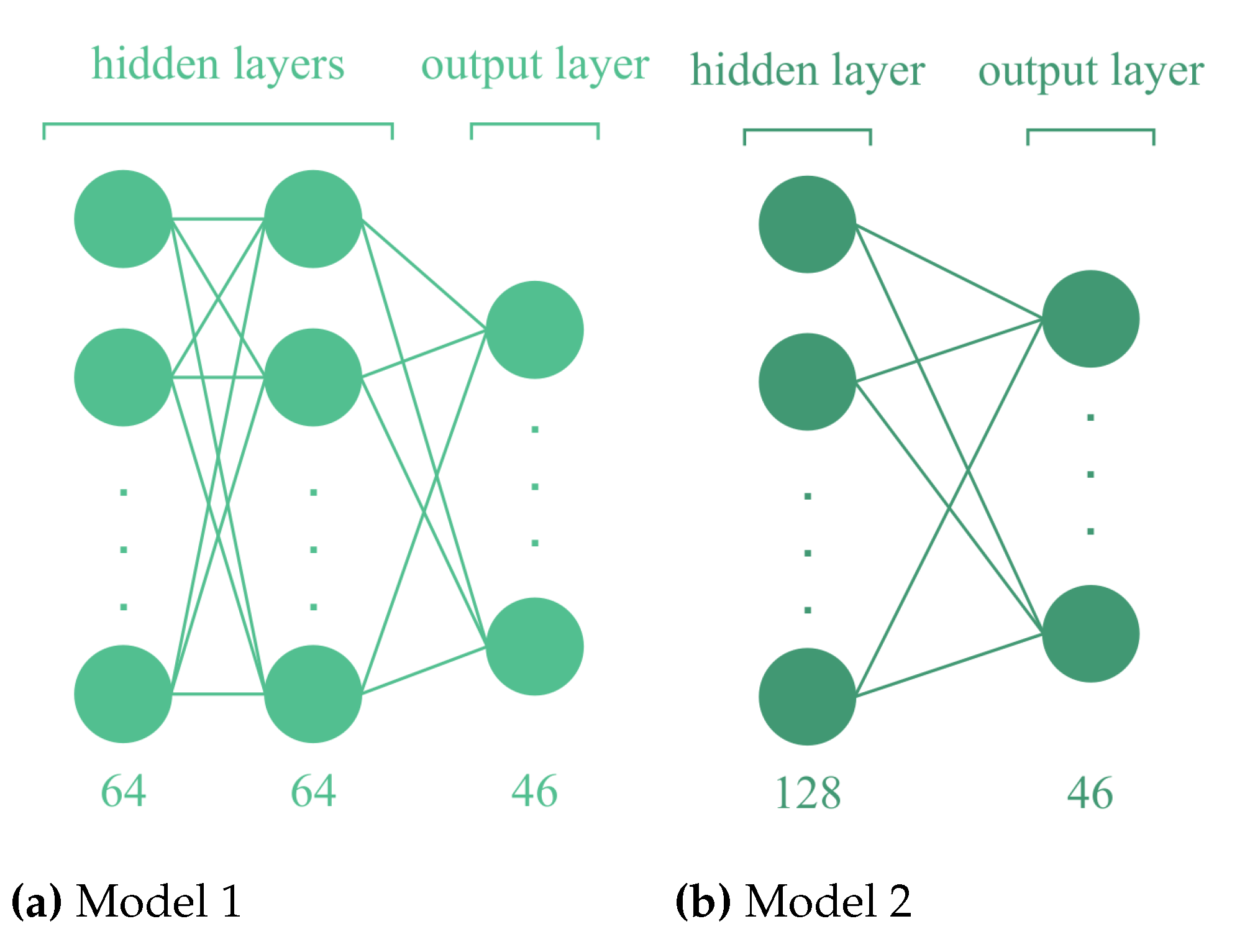
Figure 3.
Two different models for topic classification is presented. Figure 3 shows the Model 1’s architecture and Figure 3 shows the Model 2’s architecture
5.1.1. Data Preprocessing
Data preprocessing is an essential step in the data analysis and modeling processes as it ensures that the data is in the computable format for the model to analyze. This is particularly important for text data, which can be highly unstructured and contain noise such as emotions, punctuation, and misspellings. To address this, various natural language processing techniques can be applied, such as stemming, tokenization, lemmatization, removal of stop words, punctuation, extra spaces, and letter lowering. The specific techniques used will depend on the nature of the data and the problem being addressed. The Reuters Newswire Classification dataset [10] was used to perform a solution to the topic classification problem. Since the dataset was generated from the Reuters-21578 dataset, tokenization was applied only as a preprocessing step. After that list of sequences was converted to the array.
5.1.2. Models
There are two main components for training high-performance models which are data and hyperparameters. Preparing data for the model is explained in Section 5.1.1. In terms of model performance, hyperparameter tuning is a crucial step for the perfect fit and hyperparameters that will be tuned must be selected carefully according to the problem and the data.
In this experiment, two deep learning models were trained for the classification problem for observing the effects of activation functions. The first model (Model 1) is a deep neural network that has two hidden layers with 64 neurons. The second model (Model 2) is also a deep neural network that has one hidden layer with 512 neurons. Since experiments explained in the paper are about the effectiveness of activation functions, other hyperparameters were fixed. Moreover, since the problem itself is a multiclass classification, the output layer’s activation function was set to softmax. Some important hyperparameters used in the Model 1 are batch size is 512, and dropout probability is 0.4. In Model 2, the batch size is 32, and the dropout probability is 0.5. Both models have early stopping and also learning rates. The main difference between models is layer and neuron size. In Model 1, the neural network is narrower than in Model 2. It is important to use early stopping since it prevents the model from over-fitting.
5.2. Time Series Prediction
Time series prediction is an important problem for researchers and sector employees. Since modeling the time series is useful for future planning, budget planning, etc. In this work, we used day ahead market/trade value [30] in Türkiye, where the data is available at EXIST Transparency Platform. The dataset has an hourly frequency and its range is starting on October 1st, 2022 00:00, and ending on 12th December 2022 23:00. To sum up, the problem we consider here is the time-dependent univariate series. Before moving on to the model, the dataset needs to be preprocessed for the prediction problem since the features depend on the time and seasonality.
5.2.1. Data Preprocessing
Univariate time series problems generally need to extract features such as date-time, lags, etc. In our problem, we need to extract serial dependence and time-dependent properties. Serial dependence properties are obtained using the past values of the target variable. PACF and ACF plots are useful for understanding consecutive relationships between variables. It is observable that the data have 24 hours cyclic pattern at the ACF plot. Also, we observe that the time t+1’s variable is highly correlated with the time t’s variable. Moreover, one of the main feature extraction is lagging which is shifting values forward one or more time steps. Lagging is applied 36 times to the trade value to capture and learn hidden patterns. Another main feature extraction is time-dependent variables. Hour, month, year, day, week, and dayofweek independent variables are extracted from corresponding datetime information. Thus, 42 features were obtained. Since all features cannot be a helper for predictive models, feature selection is needed. Boruta, a feature selection library, was used for dimensionality reduction and feature selection. A Random Forest regression model was built with 100 estimators, and depth is 5 for the selection of features. As a result of 100 iterations, 19 features were confirmed, 3 were tentative and 20 are rejected. Features found important by Boruta are as follows: lags are 1, 2, 3, 4, 5, 7, 8, 9, 18, 21, 22, 23, 24, 26, 27, 28, 30, and time-dependent features are hour and day of the week. Finally, the MinMax scaling is applied to the dataset which is the version of the selected features since the problem we consider is a regression problem, i.e., scaling is vital. To sum up, time and serial-dependent features are extracted and selected for a univariate time series prediction.
5.2.2. Models
Time series prediction problems are based on AutoRegressive (AR) models. AR, ARMA (Auto Regressive Moving Average), ARIMA (Auto Regressive Integrated Moving Average), and MA (Moving Average) are some examples. In our case, we modeled the problem using DNN architecture to show that our promising activation functions are applicable to time series prediction problems.
In the previous section, data preprocessing steps were explained in detail. In this section, we will give details of prediction models. We applied two different models. Firstly, the dataset was divided into the train, validation, and test sets. The train set has approximately 55% set of attributes, and validation and test sets have approximately 22% a set of attributes. The first model is designed as two hidden layers with 0.2 dropout probability and 64 neurons in each and output layer with one neuron DNN model, see Figure 4. It trained with a 0.01 learning rate. The second model has 4 hidden layers with 104, 72, 184, and 104 neurons and 0.1, 0.2, 0.5, and 0.3 dropout probabilities respectively and one output layer with 1 neuron, see Figure 4. It trained with a 0.005 learning rate. Adam as an optimizer and mean squared error as a loss function were used for both models. Also, early stopping with 5 patience was used in both models.
6. Results
In this section, we will discuss the results of our experimentation with various activation functions applied to two different problems, including their impact on model training time, model performance, and the trade-offs between them.
First of all, evaluating training time is important for deep learning problems since less training time is preferable in terms of optimized solutions and energy requirements. In the topic classification problem, all promised arctan’s variations are faster than sigmoid for both models, see Figure 5. For Model 1, the best epoch size occurs for self-arctan which is faster than sigmoid, the same with tanh, and slower than the other existing activation functions. On the other hand, promised activation functions, other than self-arctan, are slower than the existing ones. For Model 2, arctan and arctan e are the slowest after sigmoid. However, arctan and self-arctan have the same epoch size with ReLU, swish, and arctan. Next, in the time series prediction problem, the slowest one is arctan for both models. For Model 1, self-arctan is the fastest between promised activation functions and it is faster than leaky ReLU and sigmoid. For Model 2, arctan is the fastest between promised ones and it is faster than only sigmoid.
Secondly, model performances are evaluated. For the first problem, topic classification, macro, and weighted average scoring methods were considered. Weighted and macro averages are considered separately since the dataset used in the problem has an unbalanced structure. For both models, promised activation functions to perform that they can compete with widely used activation functions. More specifically, in Table 2 and in Table 3 precision, recall, and F1 scores are shown. For Model 1, it can be observed that arctan is the most competitive among the promised functions. It shares the best score in weighted recall with the evaluation according to two decimal truncation. However, arctan is the worst among them and it is better than only sigmoid. For Model 2, arctan e has the best precision according to the macro average, arctan has the best recall, and F1 score according to the macro average and precision and recall according to the weighted average. Furthermore, promised activation functions are mostly better than sigmoid. As a second problem, we trained the energy trade value and evaluate them according to RMSE, MSE, and R2 score; Table 4 and Table 5. Similarly, with the first problem, we obtained competitive results. For Model 1, arctan e is the most successful among the promising activation functions. Also, it performed better than sigmoid, tanh, ReLU, and arctan for all evaluation metrics except for arctan in MSE, where they are equal at the second decimal. For Model 2, similar results were obtained, which is arctan e is the best between arctan variations.
Overall, we can conclude that
- At least one of promised activation functions beat the sigmoid in every case;
- It is significant to gain attention to functions’ range for solving problems with deep learning;
- Arctan is the best for the multiclass classification problem;
- Arctan e is the best for the time series prediction problem;
- Promising activation functions are shown that they can learn stably with different neuron numbers and model depths.
7. Discussion
The field of neural networks has seen many advancements in the last decade, one of which is the introduction of new activation functions. These functions play a crucial role in determining the output of a neuron, and as such, have a significant impact on the performance of a neural network. Many studies have focused on developing activation functions by applying different strategies like a combination of multiple functions. In this work, we mainly focused on a unique strategy which is changing the range of arctan functions with irrationals, pi, the golden ratio, the Euler number, and multiplying input with the arctan function. Furthermore, two different datasets and two different models in each are taken into consideration. One of them is the REUTERS Newswire classification dataset and the other is the Türkiye energy trade market value. Each problem has its own challenges in terms of training and data preprocessing steps. Promised activation functions are experimented on wider and narrower DNNs to see that how the results are affected by the functions’ range. As a result, it is observed that promised activation functions showed stable results. Arctan shows the most promising results on the topic classification problem and arctan e shows on the time series prediction problem. Additionally, we can mention that although there is a small difference between the ranges of arctan and e, arctan e is preferable for time series prediction. Also, arctan which has a wider range according to variations and a narrower range according to arctan itself is more successful for topic classification.
To sum up, these new activation functions have shown promising results and have the potential to improve the performance of neural networks. Further research and experimentation are needed to fully understand their advantages and limitations, as well as to determine their suitability for various tasks.
Author Contributions
Conceptualization, T.T.S.; methodology, T.T.S; software, T.T.S.; validation, T.T.S, N.P.A. and A.B.; formal analysis, T.T.S. and N.P.A.; investigation, T.T.S.; resources, T.T.S.; data curation, T.T.S.; writing—original draft preparation, T.T.S. and N.P.A.; writing—review and editing, T.T.S. and N.P.A.; visualization, T.T.A; supervision, N.P.A. and A.B.; project administration, A.B.; funding acquisition, A.B. All authors have read and agreed to the published version of the manuscript.
Funding
This research received no external funding
Institutional Review Board Statement
Not applicable.
Informed Consent Statement
Not applicable.
Data Availability Statement
EXIST Market Trade Value Dataset:https://seffaflik.epias.com.tr/transparency/piyasalar/gop/islem-hacmi.xhtml, REUTERS Newswire Dataset: https://keras.io/api/datasets/reuters
Acknowledgments
Thank you for the support to BITES Defence and Information System Department
Conflicts of Interest
The authors declare no conflict of interest.
Abbreviations
| EXIST | Energy Exchange Istanbul |
| RMSE | Root Mean Squared Error |
| MSE | Mean Squared Error |
| PACF | Partial Auto Correlation Function |
| ACF | Auto Correlation Function |
| DNN | Deep Neural Network |
| ReLU | Rectified Linear Unit |
| FCNN | Full Connected Neural Network |
| CNN | Convolutional Neural Network |
| LSTM | Long Short-Term Memory |
References
- Sivri, T. T. , Akman, N. P., & Berkol, A. (2022, June). Multiclass Classification Using Arctangent Activation Function and Its Variations. 2022 14th International Conference on Electronics, Computers and Artificial Intelligence (ECAI); IEEE; pp. 1–6.
- Sivri, T. T., Akman, N. P., Berkol, A., and Peker, C. (2022). Web Intrusion Detection Using Character Level Machine Learning Approaches with Upsampled Data. Annals of Computer Science and Information Systems 2022, 32, 269–274.
- Kamruzzaman, J. (2002). Arctangent Activation Function to Accelerate Backpropagation Learning. IEICE TRANSACTIONS on Fundamentals of Electronics. Communications and Computer Sciences 2002, E85(A), 2373–2376. [Google Scholar]
- Sharma, S.; Sharma, S.; Athaiya, A. Activation Functions In Neural Networks. International Journal of Engineering Applied Sciences and Technology 2020, 4(12), 310–316. [Google Scholar] [CrossRef]
- Paul, D., Sanap, G., Shenoy, S., Kalyane, D., Kalia, K., and Tekade, R. K. (2021). Artificial intelligence in drug discovery and 407 development. Drug discovery today, 26(1), 80–93. [CrossRef]
- B. Kisačanin, "Deep Learning for Autonomous Vehicles," 2017 IEEE 47th International Symposium on Multiple-Valued Logic (ISMVL), 2017, pp. 142-142. [CrossRef]
- D. W. Otter, J. R. D. W. Otter, J. R. Medina and J. K. Kalita, "A Survey of the Usages of Deep Learning for Natural Language Processing," in IEEE Transactions on Neural Networks and Learning Systems, vol. 32, no. 2, pp. 604-624, Feb. 2021. [CrossRef]
- Riccardo Miotto, Fei Wang, Shuang Wang, Xiaoqian Jiang, Joel T Dudley, Deep learning for healthcare: review, opportunities and challenges, Briefings in Bioinformatics, Volume 19, Issue 6, November 2018, Pages 1236–1246. 20 November. [CrossRef]
- Lee, S.I. , Yoo, S.J. Multimodal deep learning for finance: integrating and forecasting international stock markets. J Supercomput 76, 8294–8312 (2020). [CrossRef]
- Team, K. (n.d.). Keras Documentation: Reuters Newswire Classification Dataset. Keras. Retrieved December 2022, from https://keras.io/api/datasets/reuters/. 20 December.
- T. Kim and T. Adali, "Complex backpropagation neural network using elementary transcendental activation functions," 2001 IEEE International Conference on Acoustics, Speech, and Signal Processing. Proceedings (Cat. No.01CH37221), 2001, pp. 1281-1284 vol.2. [CrossRef]
- Cybenko, G. Approximation by superpositions of a sigmoidal function. Math. Control, Signals Syst. 1989, 2, 303–314. [Google Scholar] [CrossRef]
- K. Hornik, M. Stinchcombe, and H. White, “Multilayer feedforward networks are universal approximators. Neural Netw 1989, 2, 359–366. [CrossRef]
- Funahashi, K.I. On the approximate realization of continuous mappings by neural networks. Neural Netw. 1989, 2, 183–192. [Google Scholar] [CrossRef]
- A. R. Barron, “Universal approximation bounds for superpositions of a sigmoidal function. IEEE Trans. Inf. Theory, 19 May 1993; 39, 930–945.
- M. Leshno, V. Y. M. Leshno, V. Y. Lin, A. Pinkus, and S. Schocken, “Multilayer feedforward networks with a nonpolynomial activation function can approximate any function. Neural Netw. 1993; 6, 861–867. [Google Scholar]
- Misra, D. (2020). Mish: A Self Regularized Non-Monotonic Activation Function. British Machine Vision Conference.
- Parhi, R., and Nowak, R. D. (2020). The role of neural network activation functions. IEEE Signal Processing Letters, 27, 1779–1783. [CrossRef]
- Kulathunga, N. , Ranasinghe, N. R., Kinsman, Z., Vrinceanu, D., Huang, L., and Wang, Y. (2020). Effects of the Nonlinearity in Activation Functions on the Performance of Deep Learning Models. CoRR, abs/2010.07359.
- LeCun, Y.; Boser, B.; Denker, J.S.; Henderson, D.; Howard, R.E.; Hubbard, W.; et al. Backpropagation applied to handwritten zip code recognition. Neural Comput. 1989, 1, 541–551. [Google Scholar] [CrossRef]
- Sharma, O. A new activation function for deep neural network. 2019 International Conference on Machine Learning, Big Data, Cloud and Parallel Computing (COMITCon). [CrossRef]
- Liew, S. S., Khalil-Hani, M.,and Bakhteri, R. (2016). Bounded activation functions for enhanced training stability of deep neural networks on visual pattern recognition problems. Neurocomputing, 216, 718–734. [CrossRef]
- Efe, M. Ö. (2008). Novel neuronal activation functions for Feedforward Neural Networks. Neural Processing Letters, 28(2), 63–79. [CrossRef]
- Skoundrianos, E.N.; Tzafestas, S.G. Modelling and FDI of dynamic discrete time systems using a MLP with a new sigmoidal activation function. J Intell Robotics Syst 2004, 19–36. [Google Scholar] [CrossRef]
- Shen, S.-L., Zhang, N., Zhou, A., Yin, Z.-Y. (2022). Enhancement of neural networks with an alternative activation function tanhLU. Expert Systems with Applications, 199, 117181. [CrossRef]
- Augusteijn, M. F.,and Harrington, T. P. (2004). Evolving transfer functions for Artificial Neural Networks. Neural Computing and Applications, 13(1), 38–46. 1). [CrossRef]
- Benítez, José Manuel, Juan Luis Castro, and Ignacio Requena. "Are artificial neural networks black boxes? IEEE Transactions on neural networks 1997, 8, 1156–1164. [CrossRef] [PubMed]
- Jin, J. , Zhu, J., Gong, J. et al. Novel activation functions-based ZNN models for fixed-time solving dynamirc Sylvester equation. Neural Comput & Applic 34, 14297–14315 (2022). [CrossRef]
- Wang, X.; Ren, H.; Wang, A. Smish: A Novel Activation Function for Deep Learning Methods. Electronics 2022, 11, 540. [Google Scholar] [CrossRef]
- Trade Value - Day Ahead Market - Electricity Markets| EPIAS Transparency Platform. (n.d.). Retrieved December 20, 2022, from https://seffaflik.epias.com.tr/transparency/piyasalar/gop/islem-hacmi.xhtml.
Figure 4.
Two different models for trade value prediction is presented. Figure 4 shows the Model 1’s architecture and Figure 4 shows the Model 2’s architecture
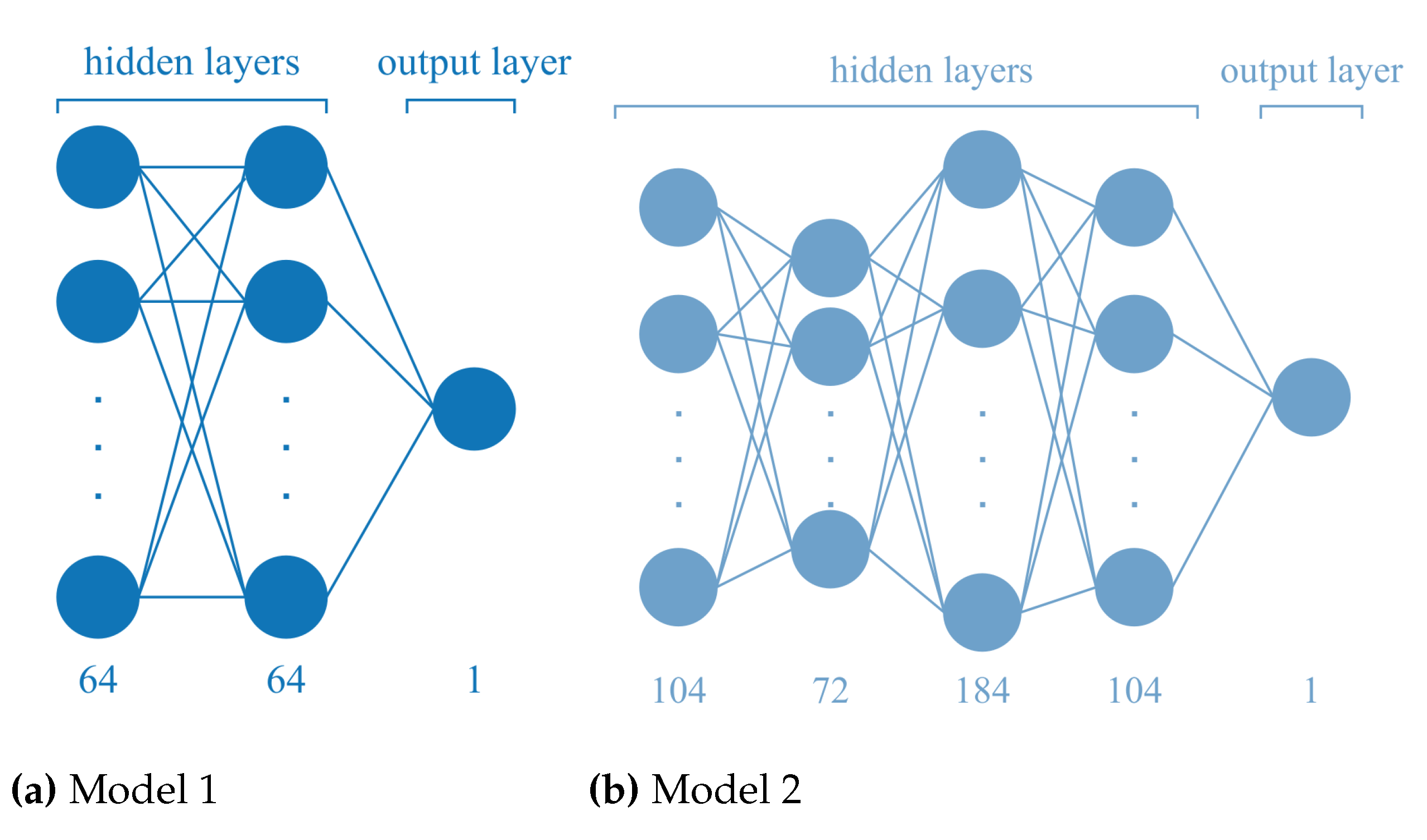
Figure 5.
Topic classification models’ epoch sizes

Figure 6.
Energy trade value models’ epoch sizes

Table 2.
Topic classification Model 1 results
| Evaluation Metrics | sigmoid | tanh | relu | leaky relu | swish | arctan | arctan | arctan | arctan e | self arctan |
|---|---|---|---|---|---|---|---|---|---|---|
| Precision1 | 0.29 | 0.65 | 0.41 | 0.61 | 0.62 | 0.67 | 0.36 | 0.61 | 0.48 | 0.40 |
| Recall1 | 0.25 | 0.45 | 0.32 | 0.42 | 0.43 | 0.45 | 0.31 | 0.44 | 0.38 | 0.29 |
| F1Score1 | 0.25 | 0.50 | 0.35 | 0.46 | 0.47 | 0.50 | 0.31 | 0.48 | 0.40 | 0.31 |
| Precision2 | 0.71 | 0.78 | 0.74 | 0.77 | 0.78 | 0.78 | 0.73 | 0.77 | 0.75 | 0.74 |
| Recall2 | 0.76 | 0.79 | 0.77 | 0.78 | 0.79 | 0.79 | 0.76 | 0.79 | 0.78 | 0.77 |
| F1Score2 | 0.72 | 0.77 | 0.75 | 0.77 | 0.77 | 0.78 | 0.74 | 0.77 | 0.76 | 0.77 |
1 Macro average 2 Weighted average
Table 3.
Topic classification Model 2 results
| Evaluation Metrics | sigmoid | tanh | relu | leaky relu | swish | arctan | arctan | arctan | arctan e | self arctan |
|---|---|---|---|---|---|---|---|---|---|---|
| Precision1 | 0.72 | 0.71 | 0.71 | 0.72 | 0.71 | 0.69 | 0.74 | 0.72 | 0.75 | 0.71 |
| Recall1 | 0.49 | 0.54 | 0.54 | 0.52 | 0.55 | 0.55 | 0.53 | 0.56 | 0.53 | 0.53 |
| F1Score1 | 0.55 | 0.58 | 0.57 | 0.58 | 0.59 | 0.59 | 0.59 | 0.60 | 0.58 | 0.57 |
| Precision2 | 0.79 | 0.80 | 0.80 | 0.79 | 0.80 | 0.80 | 0.80 | 0.81 | 0.80 | 0.80 |
| Recall2 | 0.79 | 0.80 | 0.80 | 0.80 | 0.81 | 0.80 | 0.80 | 0.81 | 0.80 | 0.80 |
| F1Score2 | 0.78 | 0.79 | 0.78 | 0.79 | 0.80 | 0.79 | 0.79 | 0.80 | 0.79 | 0.79 |
1 Macro average 2 Weighted average
Table 4.
Time series prediction Model 1 results
| Evaluation Metrics | sigmoid | tanh | relu | leaky relu | swish | arctan | arctan | arctan | arctan e | self arctan |
|---|---|---|---|---|---|---|---|---|---|---|
| RMSE | 0.17 | 0.19 | 0.18 | 0.12 | 0.12 | 0.17 | 0.43 | 0.25 | 0.14 | 0.39 |
| MSE | 0.03 | 0.03 | 0.03 | 0.01 | 0.01 | 0.02 | 0.19 | 0.06 | 0.02 | 0.15 |
| R2 score | 0.63 | 0.54 | 0.61 | 0.82 | 0.82 | 0.66 | -1.20 | 0.22 | 0.74 | -0.76 |
Table 5.
Time series prediction Model 2 results
| Evaluation Metrics | sigmoid | tanh | relu | leaky relu | swish | arctan | arctan | arctan | arctan e | self arctan |
|---|---|---|---|---|---|---|---|---|---|---|
| RMSE | 0.18 | 0.20 | 0.23 | 0.13 | 0.12 | 0.17 | 0.42 | 0.27 | 0.14 | 0.38 |
| MSE | 0.03 | 0.04 | 0.05 | 0.01 | 0.01 | 0.02 | 0.18 | 0.07 | 0.02 | 0.15 |
| R2 score | 0.61 | 0.50 | 0.34 | 0.79 | 0.80 | 0.65 | -1.12 | 0.14 | 0.76 | -0.74 |
Disclaimer/Publisher’s Note: The statements, opinions and data contained in all publications are solely those of the individual author(s) and contributor(s) and not of MDPI and/or the editor(s). MDPI and/or the editor(s) disclaim responsibility for any injury to people or property resulting from any ideas, methods, instructions or products referred to in the content. |
© 2023 by the authors. Licensee MDPI, Basel, Switzerland. This article is an open access article distributed under the terms and conditions of the Creative Commons Attribution (CC BY) license (http://creativecommons.org/licenses/by/4.0/).
Copyright: This open access article is published under a Creative Commons CC BY 4.0 license, which permit the free download, distribution, and reuse, provided that the author and preprint are cited in any reuse.


