

Submitted:
04 September 2023
Posted:
05 September 2023
Read the latest preprint version here
Abstract
A new coordinate system based on the proper times of rest frames in the Schwarzschild metric is developed to show that a radially falling worldline becomes light-like at the event horizon in the Schwarzschild metric. This system has no coordinate singularity at the event horizon and light travels on 45 degree lines everywhere in the space. The light-like nature of the worldline is confirmed by analyzing it in Kruskal-Szekeres (KS) coordinates. It is shown that the worldline in KS coordinates has an undefined derivative at the horizon at any point other than the origin of the KS coordinates. It is then demonstrated that the origin of the KS coordinate system can be reached in the falling frame by exploiting the time symmetry of the manifold and that the falling worldline is indeed light-like there. The light-like nature of the worldline means that the horizon is length contracted to a point in the falling frame, such that the event horizon is proven to be the source of the Schwarzschild metric and the end point of gravitational collapse.
Keywords:
Black holes
; General Relativity
; Schwarzschild metric
1. Introduction
The Schwarzschild metric in Schwarzschild coordinates has a well-known coordinate singularity at the event horizon. This singularity is removed from the metric using coordinate transformations, with the most popular transformation being the Kruskal-Szekeres coordinates, which are regular at the horizon. However, the meaning of the the Kruskal-Szekeres coordinates in terms of spacelike and timelike basis vectors is not clear. For much of the spacetime, the Kruskal-Szekeres coordinates are mixtures of space and time such that the meaning of the slope of a worldline in these coordinates is not always clear. Nonetheless, these coordinates have been used to argue that the event horizon can be crossed by falling observers since there is no coordinate singularity in the Kruskal-Szekeres system. This has led to the acceptance of the existence of Black Holes into which objects can fall and can never escape back out to the external Universe.
In the reference text ’Gravitation’[1], the authors depict a falling worldline crossing the event horizon in Kruskal-Szekeres coordinates in Figure 32.1(b) of the text, though there is no accompanying calculation of the worldline in Kruskal-Szekeres coordinates. The only such calculation found in the literature is in [2], where the author claims to demonstrate that all worldlines are null at the horizon in Kruskal-Szekeres coordinates regardless of their state of motion. However, as the author notes in that work, the proof actually demonstrates that the Kruskal-Szekeres derivative of the falling worldline is undefined at in Kruskal-Szekeres coordinates. The author nonetheless concludes that in order for the extended spacetime to be consistent, the geodesic must in fact be null at the horizon.
The existence of Black Holes that can subsequently evaporate create an information paradox where information falling into a Black Hole is lost once the Black Hole evaporates due to Hawking radiation. Therefore, the possibility of objects falling into a Black Hole creates a physical paradox which has yet to be conclusively resolved.
If nothing was able to fall past the event horizon of the Schwarzschild metric, then there would be no information paradox to begin with. Therefore, this paper provides proof of the following hypothesis:
- The worldline of radially falling frames become null at the event horizon and the horizon itself becomes length contracted to a point in the falling frame as it approaches the horizon. The consequence of this is that the event horizon is the source of the Schwarzschild metric and the end point of gravitational collapse
To prove this hypothesis, we first create a coordinate system where the time coordinate for the system represents the local proper time of an observer at rest at each r. This coordinate system has no coordinate singularity at the horizon and light travels on 45 degree lines everywhere in this system. By analyzing radial infall in this system, it is shown that the falling worldline becomes light-like at the horizon.
The falling worldline is then examined in Kruskal-Szekeres coordinates and we find that the Kruskal-Szekeres coordinate derivative is undefined at the horizon everywhere except at . Using the hyperbolic symmetry of the Kruskal-Szekeres coordinates that comes from the time translation symmetry of the manifold, it is shown that the point is reachable by continuously hyperbolically rotating the spacetime as the frame falls and that this construction is equivalent to describing the falling frame in Schwarzschild coordinates. When taking this approach, it is shown that even in Kruskal-Szekeres coordinates, the falling frame becomes light-like at the horizon (which must be true since a null worldline in one coordinate system must be null in all coordinate systems).
Therefore, in this work, the analysis done in [2] is extended, providing an unambiguous proof that one the falling worldline is null at the event horizon without having an undefined Kruskal-Szekeres derivative at the horizon.
2. The Falling Frame of the External Metric in Universal Rest Frame Coordinates
The Schwarzschild metric is the simplest non-trivial solution to Einstein’s field equations. It is the metric that describes every spherically symmetric vacuum spacetime. The the external form of the metric can be expressed as:
Equation 1 is the external metric with t being the timelike coordinate and r being the spacelike coordinate. The Schwarzschild radius of the metric is given by in units with . The external metric is the metric for an eternally spherically-symmetric vacuum centered in space.
We can see in equation 1 that as , the magnitude of the basis vector goes to zero while the magnitude of goes to infinity. This location is called the ’Event Horizon’ of the metric. The behaviour of the basis vectors at this location seem to imply that there is a coordinate singularity at this location since the spacetime curvature is not infinite there.
The issue with these coordinates is that it maps the spacetime based on the frame of an observer at infinity, and in this frame, the coordinates are ill-behaved at the horizon. We can introduce new coordinates which are well behaved at the horizon that we will refer to as universal rest frame coordinates.
We construct this universal rest frame coordinate system for the metric using the coordinate for the time coordinate, and for the space coordinate. Whereas in the normal Schwarzschild coordinates the time t always represents the proper time of the infinite observer, represents the local proper time of the local rest observer at the rest observer’s location. Therefore
Likewise, the coordinate comes from the proper distance interval at constant t and such that . Integrating this expression gives:
The integration constant is zero in this case so that when . Therefore, in these coordinates the metric becomes:
This is a pseudo-Minkowski metric. It differs from the Minkowski metric in that the coordinate ends at and becomes imaginary for . What these coordinates do is flatten out the spacetime by locally stretching it by different amounts depending on the location in question such that the light cones are the same orientation everywhere on the grid. In Figure 1, we see three worldlines with identical proper lengths in these new coordinates on the left and with the Schwarzschild coordinate time on the right:
On the left side of Figure 1, we see the worldlines plotted in the universal rest frame coordinates (with the t coordinates shown as dashed curved lines on the chart). Light travels on 45 degree lines everywhere on this chart. On the right side of the figure, we see the same worldlines plotted in the standard Schwarzschild coordinates.
In both charts, the proper lengths of the worldlines are identical, but they seem to get longer as the horizon is approached on the right because in those coordinates, the speed of light decreases as the horizon is approached. But since the new coordinates locally deform the spacetime such that the speed of light is the same at all locations, the lines are all the same length on the left side of the figure.
Let us consider the Lorentz boosts of frames in motion relative to the rest frame. The expression for the Lorentz boost in Schwarzschild coordinates is given by:
Noting that is the proper time interval for an observer at rest at r, equation 4 can be re-expressed to give the Lorentz factor of a moving observer relative to the rest observer at r:
From our definitions of and wee see that:
Where is the local speed of light at r. Combining this with equation 5 we obtain the Lorentz factor for an observer moving with some velocity relative to the local rest observer:
Reference [3] tells us that for an observer falling from rest at is given by:
Substituting 8 into equation 6, we see that at the horizon for a free falling observer. In fact, since is the local speed of light at r which goes to zero at , for all observers at the horizon, regardless of their state of motion.
That the falling worldline approaches the speed of light at the horizon is an intuitive result. In any rest frame at some radius greater than the Schwarzschild radius, it takes an infinite amount of proper time (in the rest frame) for the falling observer to reach the horizon. But in the frame of the falling observer that started falling from some finite r, it takes a finite proper time to reach the horizon. This is possible because the speed of the falling observer relative to the rest observer at r as the falling observer passes the rest observer at r increases as the horizon is approached. Thus, the amount of elapsed proper time in the falling frame at r relative to the elapsed proper time of the rest observer at r (given by ) decreases to zero as the horizon is approached.
The fact that the falling observer approaches the speed of light as the horizon approaches also allows us to make sense of the fact that the axis ends at . Figure 2 shows the Lorentz boosted frame of the falling frame relative to the rest frames in the universal rest frame coordinates for three positions during the fall.
Since the falling frame becomes null at the horizon, the spacetime becomes infinitely length contracted in that frame due to the Lorentz boost. Since the horizon itself is at rest relative to the falling frame, the length contraction of the horizon in the falling frame becomes infinite such that the horizon becomes a point with no interior in the falling frame at the horizon. The planar surfaces perpendicular to a Cartesian coordinate axis in the Minkowski metric become spherical surfaces centered on the metric source in the Schwarzschild metric. So when we talk about length contraction in a radially falling frame, we are saying that circumferences around the source of the metric are length contracted in that frame and remain circular. This radial contraction is necessary for all inertial observers to see the spacetime as spherically symmetric. If the length contraction was dependant on the direction of the radial fall, then inertial observers would disagree on the spherical symmetry of the metric.
But to put this hypothesis on firm ground, we need to examine the falling frame in Kruskal-Szekeres coordinates, which are commonly used to visualize how the falling observer can cross the event horizon.
3. The Falling Frame of the External Metric in Kruskal-Szekeres Coordinates
The Kruskal-Szekeres coordinates are the maximally extended coordinates for the Schwarzschild metric. The coordinate definitions and metric in Kruskal-Szekeres coordinates are given below (derivation of the coordinate definitions and metric can be found in reference [4] where and ).
With the full metric in Kruskal-Szekeres coordinates given by:
Finally, we plot the metric on the Kruskal-Szekeres coordinate chart [5] in Figure 3:
In this paper, we will be focusing on region I in this chart, which is the spherically symmetric spacetime around a spherically symmetric source in space.
We can see in Figure 3 that for a rest frame (), that depends on the value of t we evaluate the derivative at since the derivative for the rest frame is the tangent to the hyperbola at t. Since the metric is time-symmetric, we know that the actual physics does not depend on the value of t and therefore, we need a deeper understanding of the meaning of the changing in the rest frame and how it relates to the falling frame at the same point.
The time symmetry of the metric tells us that we can hyperbolically rotate the spacetime (rotate the t coordinates in the coordinate chart) without changing the physics. For example, Figure 4 shows two identical worldlines hyperbolically rotated relative to each other on the Kruskal-Szekeres coordinate chart.
These worldlines are the same because and are the same for both worldlines, such that their proper lengths are the same. So the time translation symmetry of the metric translates to hyperbolic rotational symmetry on the Kruskal-Szekeres coordinate chart.
We can use this fact to change how we visualize the worldline of an observer falling toward the horizon. Rather than drawing the line from at some r to at the horizon, we can continuously hyperbolically rotate the space as the observer falls such that the ’present’ state of the falling frame is always at . An example of this is given in Figure 5.
In Figure 5, the observer begins falling at . This is represented by the rightmost point on the X axis in the diagram. After , the observer has fallen to a lower radius represented by the point to the left of the rightmost point. So rather than having the worldline grow up from as time passes, we hyperbolically rotated the worldline points down as time passes to keep the present point of the worldline on the X axis. This is a valid way of visualizing the worldline as a result of the time symmetry of the metric.
When using this construction, we see that the falling worldline reaches the point on the diagram. And if the worldline does indeed become null at the horizon, this means the worldline remains on the line since that is the null geodesic representing the horizon.
It is notable that since the lines are null geodesics at the same point in space (), this means that all falling frames reach the horizon simultaneously regardless of where or when they begin falling relative to each other. This fact is more evident when drawing the worldlines the traditional way where they reach the horizon at . If two frames start falling from different radii at , they will intersect the the horizon at at different points along the line in the coordinate chart. But the proper distance between those points is zero and they are both at the same point in space, therefore the two points are in fact coincident.
There appears to be a conflict between the construction in Figure 5 and the traditional construction which has the worldline reach the horizon at along the line where T and X are greater than zero. This conflict is significant because the construction presented here shows a worldline that becomes null at the horizon whereas the traditional construction has a non-null worldline at the horizon. It is impossible for both to be true and therefore the discrepancy must be resolved. To resolve this conflict, we need a more detailed examination of the falling frame’s worldline in Kruskal-Szekeres coordinates.
Let us first take the differentials of T and X in equations 9:
Calculating the partial derivatives, rearranging and defining we get:
Next, we need to calculate from equations 12 by factoring out from each equation and dividing:
This equation is the same equation derived in [2] but put in a slightly different form. Next, we make the following definitions:
This is the derivative of the rest frame at t since plugging into equation 13, we get . Since we know the Schwarzschild metric is independent of t, this derivative must be a non-physical artifact of the Kruskal-Szekeres coordinates at fixed r and is not related to any actual change in motion through space and time.
And we define the relative velocity of the frame in motion relative to the rest frame as:
This is the relative velocity in Kruskal-Szekeres coordinates between the frame in motion and the rest frame at r. This derivative is 0 for the rest frame since in that frame. We see also that this derivative is equal to the derivative of the universal rest frame coordinates. If we combine equations 15 and 8 we get:
Which is well behaved and equal to -1 when . Plugging these definitions into equation 13, we get:
We recognize that equation 17 is the relativistic velocity addition formula giving us the total velocity as the relativistic sum of the rest frame velocity and the relative velocity between the moving frame and the rest frame. We can solve for to get an expression for the relative velocity between a frame in motion and the rest frame in Kruskal-Szekeres coordinates:
Assuming that ranges from -1 to 1 and , we see that the relative velocity approaches 1 or -1 for all as the horizon is approached since the horizon is at , such that there. Equation 18 is also constant along a given hyperbola (i.e it is independent of t) since it represents the relative velocity between the moving and rest frames.
Equation 18 is essentially a hyperbolic rotation of a given worldline point along a hyperbola of constant r to . The reason this gives us the relative velocity is that at , the Schwarzschild basis vectors and Kruskal-Szekeres basis vectors are aligned there, meaning that the X and T in are pure spacelike and timelike basis vectors and thus the derivative gives a true velocity relative to the rest frame. This is in contrast to the general which is a derivative without a clear spacetime meaning since the X and T coordinates are mixtures of space and time everywhere else.
It is also notable that equation 17 is undefined when because since there and there, we get:
This is also what was demonstrated in [2]. Therefore, under these conditions, and are undefined at the horizon when T and X are greater than 0. This suggests that there is a discontinuity in the worldline when crossing the horizon at , even in Kruskal-Szekeres coordinates.
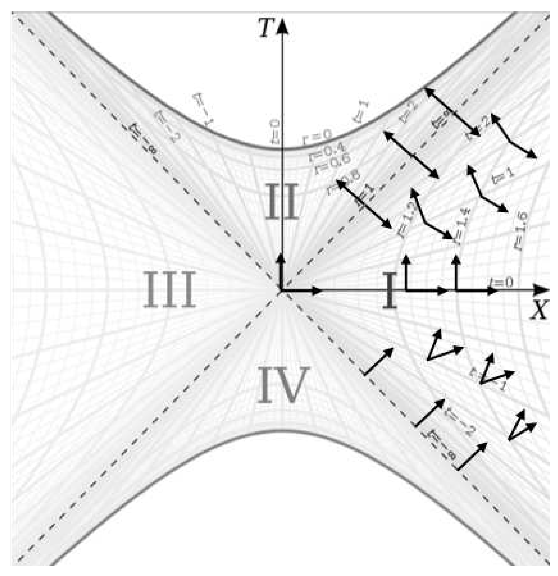
Figure 6 can help us see why equation 13 becomes undefined at the horizon by depicting the space and time axes of the rest frames at different points on the Kruskal-Szekeres coordinate chart.
Along the X axis, the space and time bases are orthogonal and aligned with the Kruskal-Szekeres basis vectors. As t moves away from 0 in either direction, the rest frames in which the derivative is measured become increasingly Lorentz boosted. These boosts are an artifact of the Kruskal-Szekeres coordinates and not physical boosts. We know this because is a Killing vector. So if we move along a hyperbola of constant r, the space-time bases are boosted as t increases, but we know that the frame of the rest observer does not change over time due to the time symmetry of the manifold.
That the derivative is measured in increasingly boosted rest frames over time in Kruskal-Szekeres coordinates is not a problem anywhere except at . At those locations, the rest frame is infinitely Lorentz boosted such that the space-time bases are collinear because the rest frame is light-like at the horizon. In a light-like frame, the relative state of motion of other frames cannot be determined because in the light like frame, one cannot make measurements of space and time due to the collinearity of the bases.
Now let’s calculate the situation described in Figure 5 where we calculate the worldline falling along the X axis as the past worldline is hyperbolically rotated down. For this construction, we set in the equations since the derivative is always taken on the X axis. For this calculation, we put the metric in the following form (we will be examining radial infall so ):
Since we are keeping , we can use the inverse of equation 16 for in the equation. We can solve for r in terms of X by setting for the X equation in equation 9 and solving for r:
Where W is the Product Log function. Substituting equations 21 and 16 into equation 20 allows us to integrate the worldline along the X axis:
Which goes to 0 as X goes to 0. But we can now show that this is exactly equivalent to falling in Schwarzschild coordinates by first using equation 12 to solve for when :
Substituting equations 23 and the inverse of 15 into equation 20 gives:
And we can see that Equation 24 is in fact the Schwarzschild metric in Schwarzschild coordinates.
Therefore it has been proven that the worldline construction shown in Figure 5 is equivalent to falling in Schwarzschild coordinates and it has been demonstrated that the worldline in that construction is light-like at the horizon. When we couple this finding with the fact that the Kruskal-Szekeres derivative is undefined at the horizon for any construction in which the worldline reaches the horizon at , we can conclude that the event horizon is contracted to a point in a falling frame approaching the horizon as a result of the fact that the worldline becomes null there.
Furthermore, we see from equation 23 that is zero at . Therefore, the falling frame remains at the horizon along the lines in the Kruskal-Szekeres coordinate chart when it reaches the horizon.
Given the above analysis, it can be concluded that the event horizon is the end point of gravitational collapse and that the source of the Schwarzschild metric is at the event horizon, more specifically the source can be visualized as the point on the Kruskal-Szekeres coordinate chart. While the event horizon is not a curvature singularity of the spacetime, it has been shown to be a discontinuity in the extended spacetime.
In a followup work, it will be shown that it is impossible to reach the event horizon due to cosmological time constraints. It will also focus on what the other three regions of the Kruskal-Szekeres chart represent as well as what is the curvature singularity and what happens there if it is not the source of the metric.
Statements and Declarations
There are no competing interests
Data Availability Statement:
All data generated or analysed during this study are included in this published article and its supplementary information files.
References
- Misner, C.; Thorne, K.; Wheeler, J. Gravitation; Number pt. 3 in Gravitation, W. H. Freeman, 1973.
- Mitra, A. Kruskal Dynamics for Radial Geodesics. International Journal of Astronomy and Astrophysics 2012, 2, 174–179. [CrossRef]
- Raine, D.; Thomas, E. Black Holes a Student Text; Imperial College Press, 2015.
- Carroll, S.M. Lecture Notes on General Relativity, 1997, [arXiv:gr-qc/9712019v1].
- Figures 3, 4, and 5 are modifications of: ’Kruskal diagram of Schwarzschild chart’ by Dr Greg. Licensed under CC BY-SA 3.0 via Wikimedia Commons. http://commons.wikimedia.org/wiki/File:Kruskal_diagram_of_Schwarzschild_chart.svg#/media/File:Kruskal_diagram_of_Schwarzschild_chart.svg, Accessed in 2017.
Figure 1.
Rest Observer Worldlines.
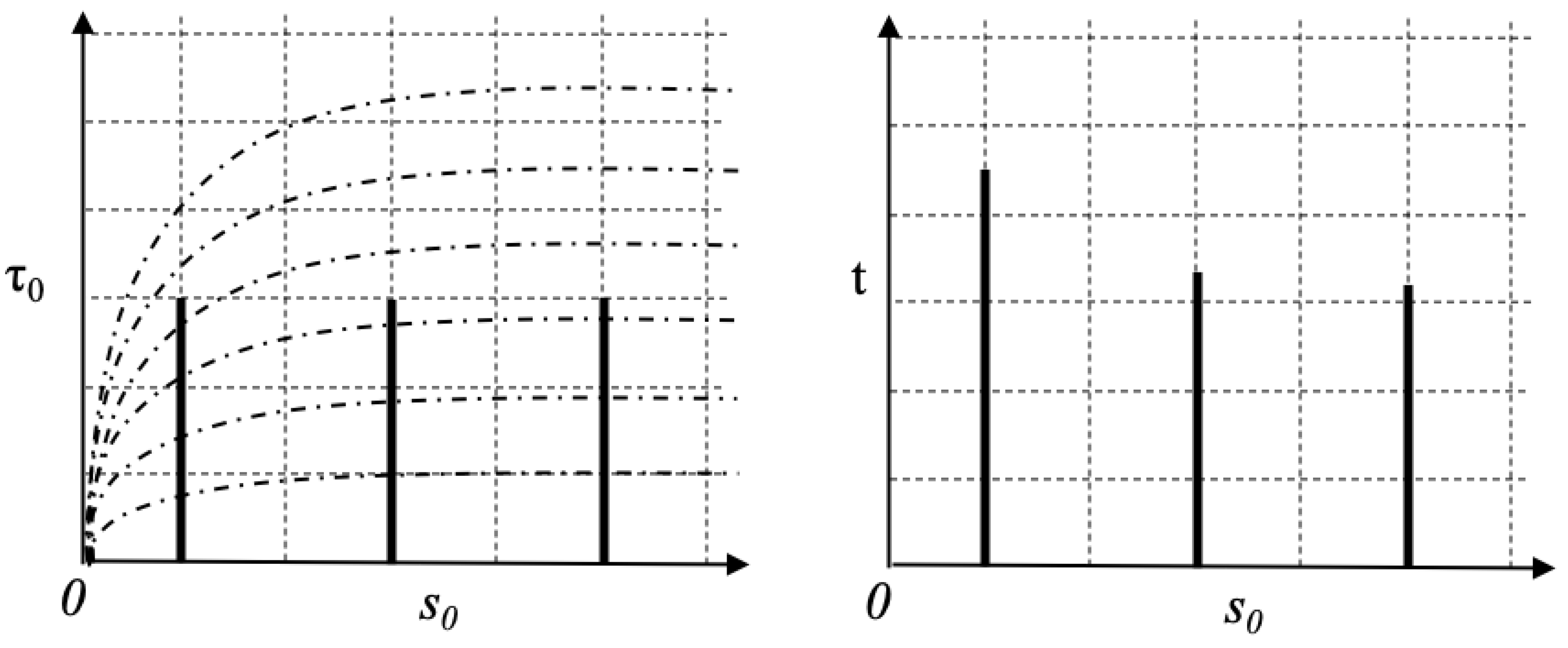
Figure 2.
Lorentz Boost of the Falling Frame Relative to the Rest Frames in the Universal Rest Frame Coordinates.
Figure 2.
Lorentz Boost of the Falling Frame Relative to the Rest Frames in the Universal Rest Frame Coordinates.
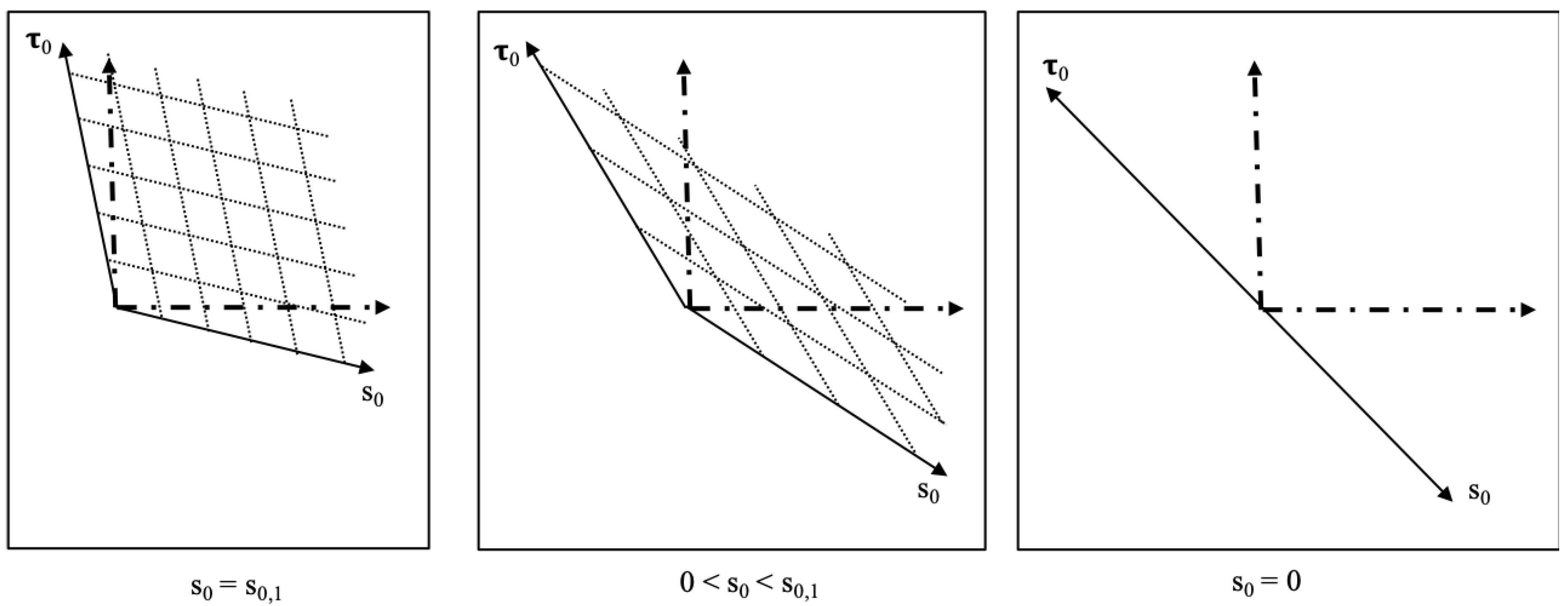
Figure 3.
Kruskal-Szekeres Coordinate Chart.
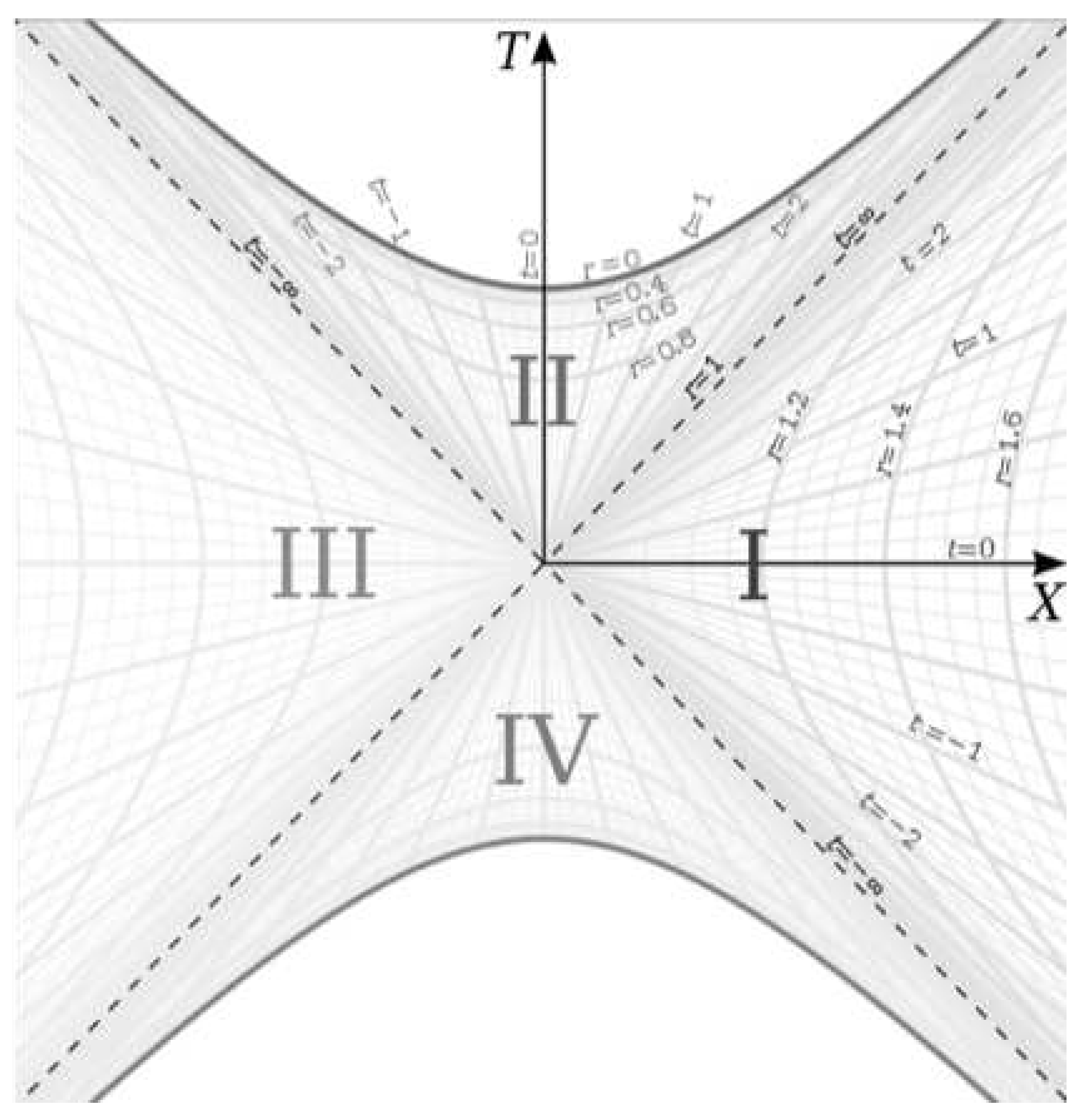
Figure 4.
Hyperbolic Rotation of a Worldline on the Kruskal-Szekeres Coordinate Chart.
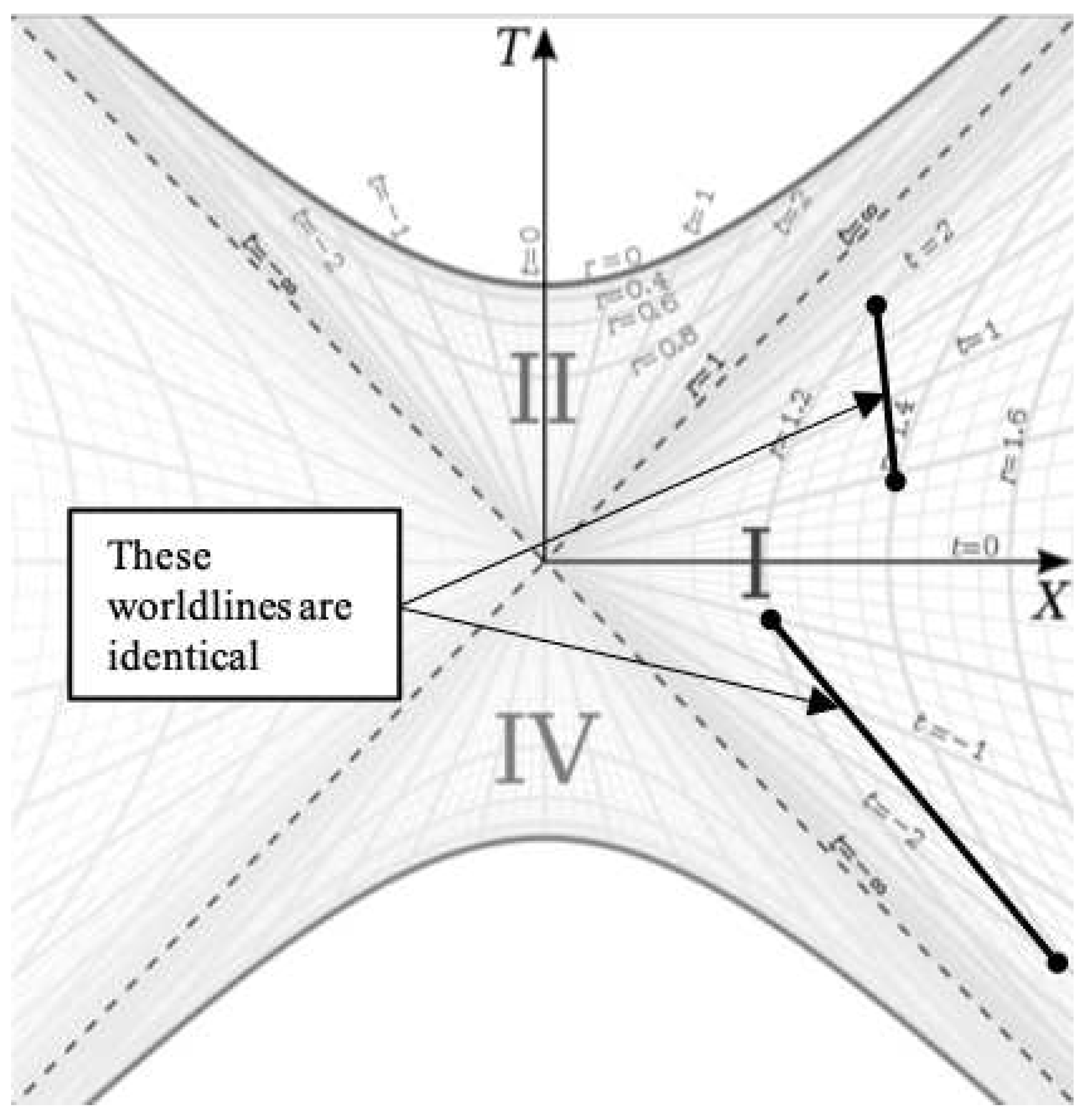
Figure 5.
Worldline of Falling Frame on the Kruskal-Szekeres Coordinate Chart with Continuous Hyperbolic Rotation.
Figure 5.
Worldline of Falling Frame on the Kruskal-Szekeres Coordinate Chart with Continuous Hyperbolic Rotation.
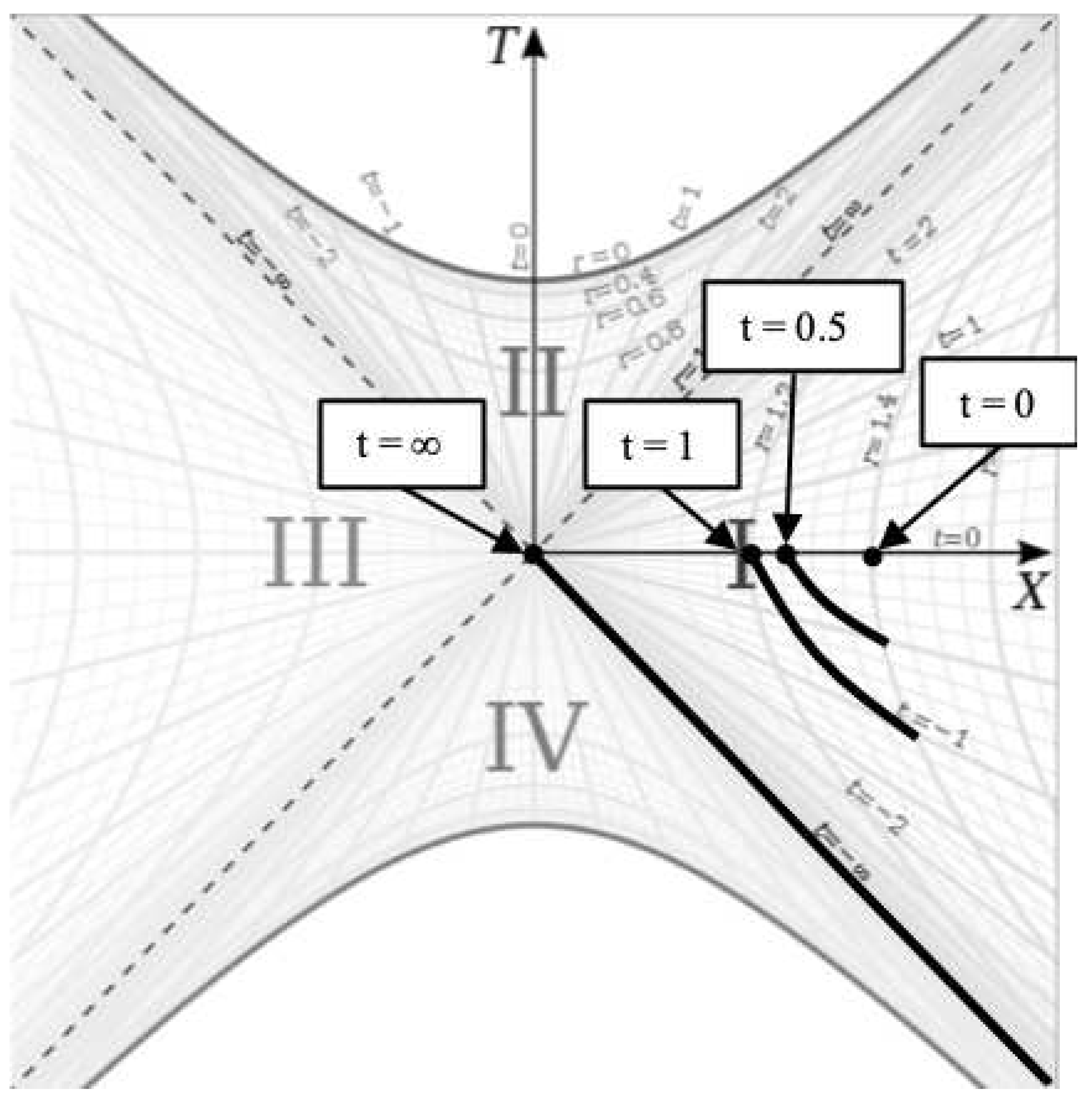
Figure 6.
Boosted Rest Frames in Kruskal-Szekeres Coordinates.
Disclaimer/Publisher’s Note: The statements, opinions and data contained in all publications are solely those of the individual author(s) and contributor(s) and not of MDPI and/or the editor(s). MDPI and/or the editor(s) disclaim responsibility for any injury to people or property resulting from any ideas, methods, instructions or products referred to in the content. |
© 2023 by the authors. Licensee MDPI, Basel, Switzerland. This article is an open access article distributed under the terms and conditions of the Creative Commons Attribution (CC BY) license (http://creativecommons.org/licenses/by/4.0/).
Copyright: This open access article is published under a Creative Commons CC BY 4.0 license, which permit the free download, distribution, and reuse, provided that the author and preprint are cited in any reuse.


