Preprint
Article

Comparative Evaluation of the Models for Predicting the Rela-Tionship Between Electrical and Chemical Properties of Engine Lubricants: An Exact Monitoring Approach

Altmetrics

Downloads

148

Views

46

Comments

0

Submitted:

13 March 2023

Posted:

17 March 2023

You are already at the latest version

Alerts
Abstract
Condition monitoring is a primary principle for predictive maintenance. In this regard, several techniques have been employed, each of which has its strengths and weaknesses. In this work, the relationships between the electrical (ε', ε", tan δ) and chemical (Fe, Pb, Cu, Cr, Al, Si, Zn) properties of engine lubricants were investigated using soft computing models. The models' performance was evaluated considering some criteria, including RMSE and MAPE. The RBF model was determined as the best one to predict chemical properties (Fe, Pb, Cu, Cr, Al, Si, Zn) through electrical indexes (ε', ε", tan δ). The RBF’s parameters (e.g., hidden size and training algorithm) were then optimized for optimum performance. For instance, in the RBF model implemented to predict Al, the best hidden size and training algorithmic were 15 and 'trainlm', respectively. Finally, by sensitivity analysis it was observed that eliminating any of the inputs does not improve the performance of the RBF model performance. In general, the results of the current research showed that the electrical properties (e.g., ε', ε", tan δ) have the capability of estimating the contaminants in the lubricants which can improve the existing monitoring methods.
Keywords: 
Subject: Engineering  -   Automotive Engineering

1. Introduction

Nowadays, high-reliable mechanical systems are expected [1]. Condition monitoring is known as a fundamental program for maintaining and assuring the safety, permanence, and performance of a machine [2,3]. Lubricant in a machine acts almost the same as blood in a living organism [4]. In other words, lubricants are responsible for many tasks like reducing friction and wear, transferring heat and energy, and reducing noise [5]. However, the primary function of a lubricant is to reduce the tribological operation problems relevant to friction and wear [6]. From maintenance point of view, oil analysis is an effective technique to evaluating the operational condition of mechanical systems [7]. The evolution of maintenance strategies over time is presented in Figure 1. Currently, there are several different methods for evaluating lubricating oil, which include [8]:
Physical and chemical methods, such as chromatography.
Spectral analysis techniques, mainly infrared absorption spectroscopy (IAS) and Raman spectroscopy.
Electrical diagnosis methods, including return voltage measurement and frequency-domain spectroscopy.
The timeline for changing and testing lubricants is a controversial issue. Although the laboratory methods can report the exact results, however they cannot determine timely maintenance [10,11]. Having this, the electrical techniques are promising methods since they provide in-situ measurement and allow easy to use and cost-effective [12,13]. On the other hand, the soft computing methods have been employed to analyze without experts [11,14,15].
Several research works on the issue of lubricant condition monitoring can be found in the literature, which are reviewed hereinafter, some of them have concentrated on modeling and using soft computing [11,16,17,18,19]. Research was recently accomplished and applied a preliminary test on engine lubricant spectral analysis based on K-nearest neighbor (KNN) and Radial Basis Function (RBF). By doing that, twelve indexes were reduced to seven indexes including iron, chromium, lead, copper, aluminum, nickel, and TDPQ. They reported that RBF-ANN modeling was able to provide detection for all three sizes of the training set with accuracy of approximately 99.85% [11]. In another study, to identify and predict external wear failure the Recursive Feature Elimination (RFE) method was used to reduce the independent variables. They could achieve the accuracy of 94.20%. They also observed that iron, aluminum, and lead were more important in assessing wear condition [18].
Dielectric or Impedance Spectroscopy (IS) is another way of measuring the electrical indexes of various materials (concrete, paper, liquids, biofuels, etc.) as an effective, economical, and non-destructive method [20]. One research has assumed a method for locomotive system maintenance. Actually, this study has studied the relationship between dielectric properties and metallic and non-metallic particles. Artificial neural networks have been employed to determine the relationship between the dielectric constant and oil impurities, and also the dielectric loss factor and oil impurities. In the modeling process, the oil impurities (chemical properties) have been considered inputs, and dielectric properties as outputs. The highest regression values (R) have been obtained for the dielectric constant (0.8513) and the dielectric loss factor (0.8015) at 7.4 GHz [11].
In this study, the primary purpose was to compare soft computing models employed to predict the chemical properties (Fe, Pb, Cu, Cr, Al, Si, Zn) of lubricants through their electrical properties (ε′, ε″, tan δ). The dataset was obtained from two sources: data extruded from other papers and data experimented in this study. More detailed information was given in Section 2. The result of this work will make to develop monitoring condition engine lubricant and promote online and portable methods for sensing and detecting faults in engine health. The research process and results are as follows.

2. Materials and Methods

2.1. Data Set

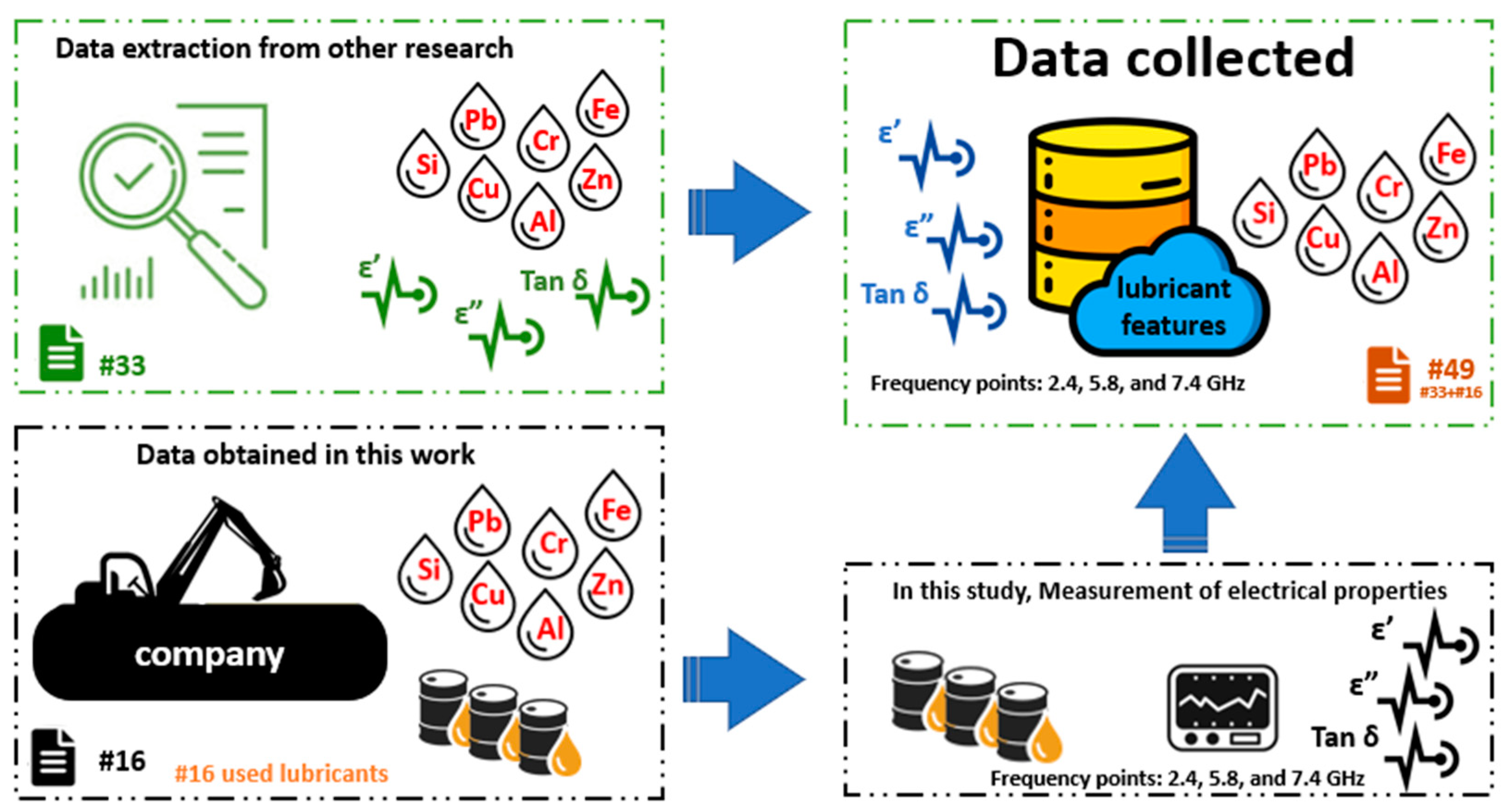
The required data set was supplied from two sources. Some of them (33 records) were extracted from previous research [10] and the rest (16 records) were provided by an Iranian company (Tirage). These records are mainly the chemical properties (Fe, Pb, Cu, Cr, Al, Si, Zn) of the lubricants. While, their electrical factors (ε′, ε″, tan δ) were measured through this work. The procedure of data collection is depicted in Figure 2. The additional information is provided in Section 2.1.1 and Section 2.1.2. To remove the effect of amplitude of changes in the values, normalization was accomplished in the range of -1 to 1 as follow [21,22]:
E n = 1 + 2 E E m i n E m a x E m i n
where, E = E 1 , E 2 ,   , E n represents the principal value of the index vector. En represents the normalized value of the index vector. Emax and Emin represent the maximum and minimum values of the index.

2.1.1. Extracted Datasets

As mentioned, the 33 records were extracted from a published work. These data included the chemical (Fe, Pb, Cu, Cr, Al, Si, Zn) and electrical properties (ε′, ε″, tan δ) of the second-hand lubricant [10]. Also, the 16 records were provided by an Iranian local company called Tirage. The lubricant samples had been picked up from engines and were shared by Tirage, along with their chemical properties (Table 1). Therefore, their electrical properties (ε′, ε″, tan δ) were measured in this work and reported in Section 2.1.2.

2.1.2. Experimental Datasets

The 16 lubricant samples that had been extracted from engines were provided by Tirage Company (Table 1). Their chemical properties including Fe, Pb, Cu, Cr, Al, Si, and Zn contents were provided by the company, however their electrical properties (e.g., ε′, ε″, tan δ) are not specified. Therefore, the electrical properties (ε′, ε″, tan δ) were measured through current research by a Vector Network Analyzer (VNA) (R&S ZVL 13, made in USA). This device can analyze microwave absorbing properties in the frequency range of 9 kHz–13.6 GHz with ±0.2 dB accuracy. The lubricant sample of 50 ml was poured into a beaker, and a coaxial dielectric probe was inserted inside the oil sample, as seen in Figure 3. The measurements were performed at 2.4, 5.8, and 7.4 GHz frequencies in triplicate, under similar conditions for all samples. The results of measurements are reported in Table 2.

2.2. Soft Computing Methods

2.2.1. Fundamentals and Theories

Soft computing models make the possibility of doing maintenance without experts. In this article, some models were designed to meet the objectives of performing maintenance and are explained below. MLP is the most commonly used type of neural network in most academic research [23,24]. In MLP, the summation functions (Eq. 2-4) is used to obtain the output of hidden neurons [25].
z j = i = 1 n 0 W i j E i + b j
y j = f z j = 1 1 + e z j
p k = j = 1 n 1 W j k y j + b k
where, z j is the input of the jth neuron in the hidden layer, b j is the bias of jth neuron in the hidden layer, W i j is the weight value between the ith input neuron and the jth neuron in the hidden layer, f z j is the activation function, y j is the outputs of jth neuron, p k is the output of the neurons in the kth output, W j k is the weight value between the neuron in the jth hidden layer and the neuron in the kth output layer, and n 1 is the number of neurons in the hidden layers. MLP commonly uses the backpropagation algorithm to find its parameters.
The Adaptive Neuro-Fuzzy Inference System (ANFIS) applies as a machine learning technique that integrates the adaptive neural network (ANN) rules and fuzzy logic (FL) theories inside an adaptive network framework to form a logical relationship between inputs and outputs [26,27]. ANFIS is a five-layered structure consisting of the fuzzy layer, product layer, normalized layer, de-fuzzy layer, and the total output layer [28].
RBF network acts as a feed-forward neural network with one hidden layer of RBF units and a linear output layer [29,30]. The output is given as [31]:
p i = b i + j = 1 N W i j exp ( E μ 2 2 σ j 2 )
where, p i is the output, b i is the bias terms, N is the number of basic functions, W i j is the weight between hidden and output layers, E is the input data vector, μ is the center of RBF unit, and σ represents the spread of the Gaussian basis function.
Support Vector Machine (SVM) was first developed by Vladimir Vapnik and further employed by others for various applications (e.g., [32]). The SVM is based on statistical learning and the estimation function of y(i) was provided as [33,34,35]:
f E = W φ E + b
where, φ E defines a nonlinear mapping of E, W is a weight vector, and b represents the bias factor.
Gaussian Process Regression (GPR) is a nonparametric Bayesian approach to regression. This method has been employed in various scientific fields [36]. GPR is providing a reliable response for the input data [37]. In Gaussian process regression, it is supposed that the output can be calculated as [38,39]:
p i = f E i + ε i               ,         ε i ~ N ( 0 , σ n o i s e 2 ) R
where, σ n o i s e 2 is the equal noise variance for E i of all samples.
The current study is focused on the soft computing approaches, however the theoretical principles of these methods are not addressed, as they can be found elsewhere in the literature. Comparing the performance of several different soft computing models as an intelligent way to improve the maintenance and monitoring of engine lubricantion conditions based on their electrical properties (ε′, ε″, tan δ).

2.2.2. Application

Considering the aforementioned section, the soft computing models were employed and their performance were comparatively evaluated to provide an innovative way for engine lubricant monitoring condition through their electrical properties (ε′, ε″, tan δ). In this regard, practical steps were performed to implement their algorithm (soft computing algorithms) in the MATLAB software. The inputs of models are the electrical properties (ε′, ε″, tan δ) of lubricants and the outputs of models are the chemical properties (Fe, Pb, Cu, Cr, Al, Si, Zn) of lubricants. The models were trained using 80% of the total data, while the rest is used for testing and validation. The optimizing indexes for the selected model were reported. The most common way to adjust model indexes is to experiment or trial and error [23].

2.3. Performance Criteria

Performance criteria must be used to evaluate the predictive accuracy of models. It will help to improve and choose the optimal model. The Mean Absolute Percentage Error (MAPE) (Eq.8) and Root Means Square Error (RMSE) (Eq.10) were used as metrics in assessing and comparing [40,41,42,43,44,45].
R M S E = i = 1 n ( y p i y e i ) 2 n
M A P E = 1 n i = 1 n y p i y e i y p i
where, y e i is the ith component of the desired (actual) output for the jth pattern, and y p i is the component of the predicted (fitted) output produced by the network for the ith pattern. The " n " is the number of lubricant samples.

3. Results and Discussion

3.1. Preliminary Statistical Analysis

Correlation is a statistical measure of how two or more variables change in connection with each other. On the other hand, it expresses the extent to which two variables are linearly related. Consequently, its results make it possible to select the best modeling method. In other words, some of the statistical models such as Multiple Linear Regression (MLR) are not appropriate when the correlation indicates a weak relation. In addition, it shows that it is a complex and non-linear issue. The closer the correlation to one, the better relation between the two variables. Also, the sign of correlation indicates a direct or inverse relationship. In this study, the best correlation observed between Zn and tan δ, and with inverse relationship. However, the least correlation achieved between Fe and ε′, and with inverse relationship. All correlations are illustrated in Table 3.

3.2. Performance Evaluation of Models

Table 4 shows the statistical analysis of the models. Comparison and judgment are possible considering the values of RMSE and MAPE. The closer the RMSE and MAPE, to zero, the better model performance. It can be seen that the smallest value of MAPE and RMSE was obtained for all variables in RBF at 7.40 GHz. For instance, RMSE and MAPE were respectively equal to 0.4 and 0.7 for Si in RBF at 7.40 GHz

3.2.1. Adjusting RBF Parameters

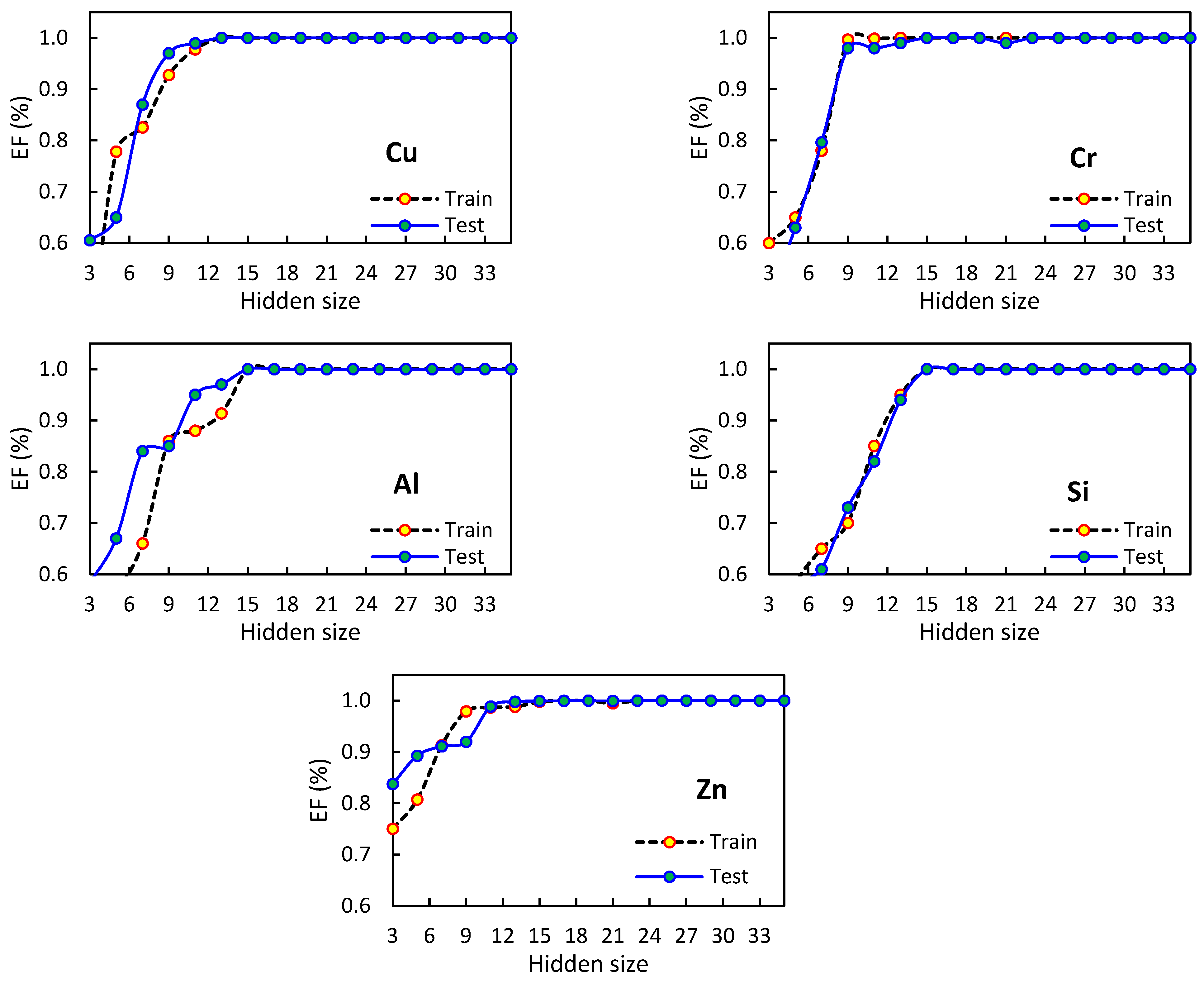
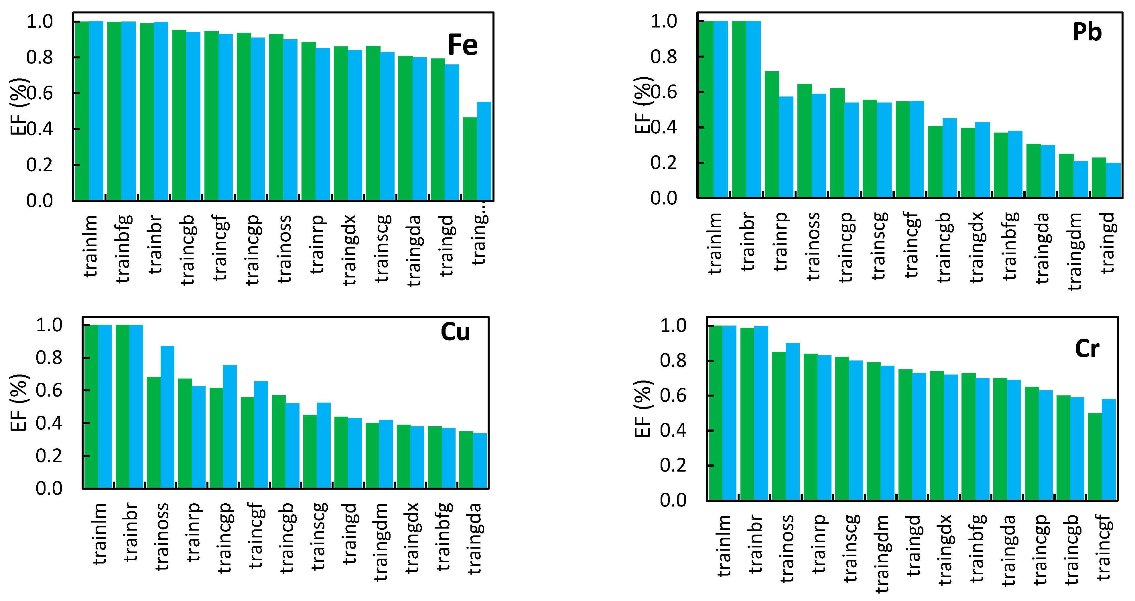
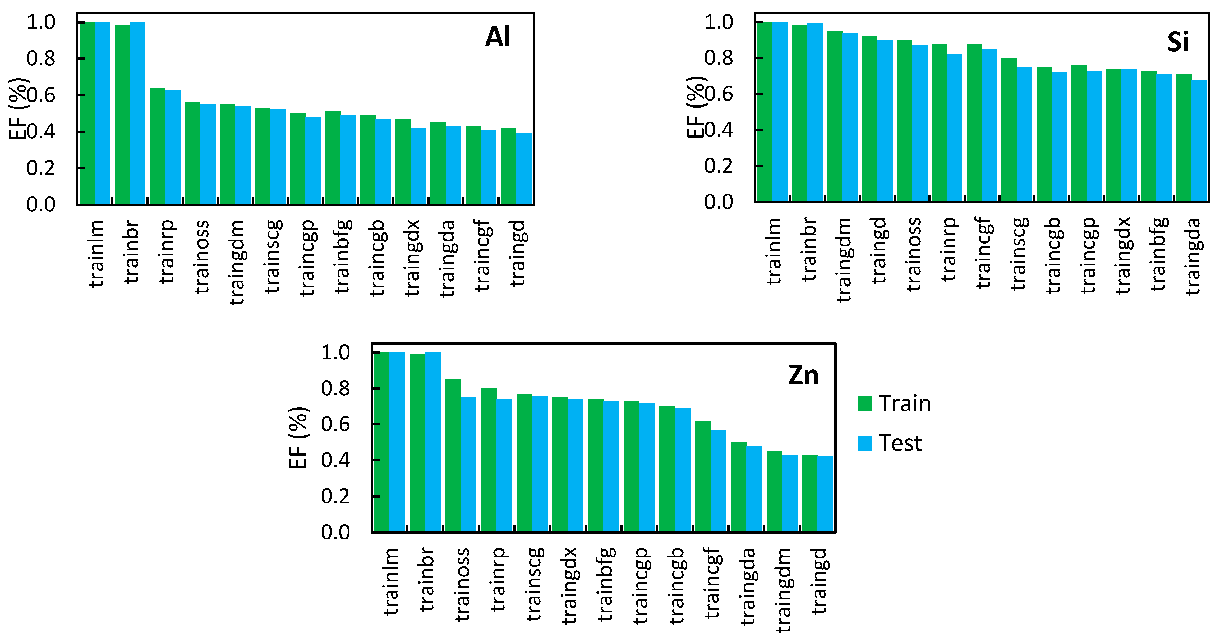
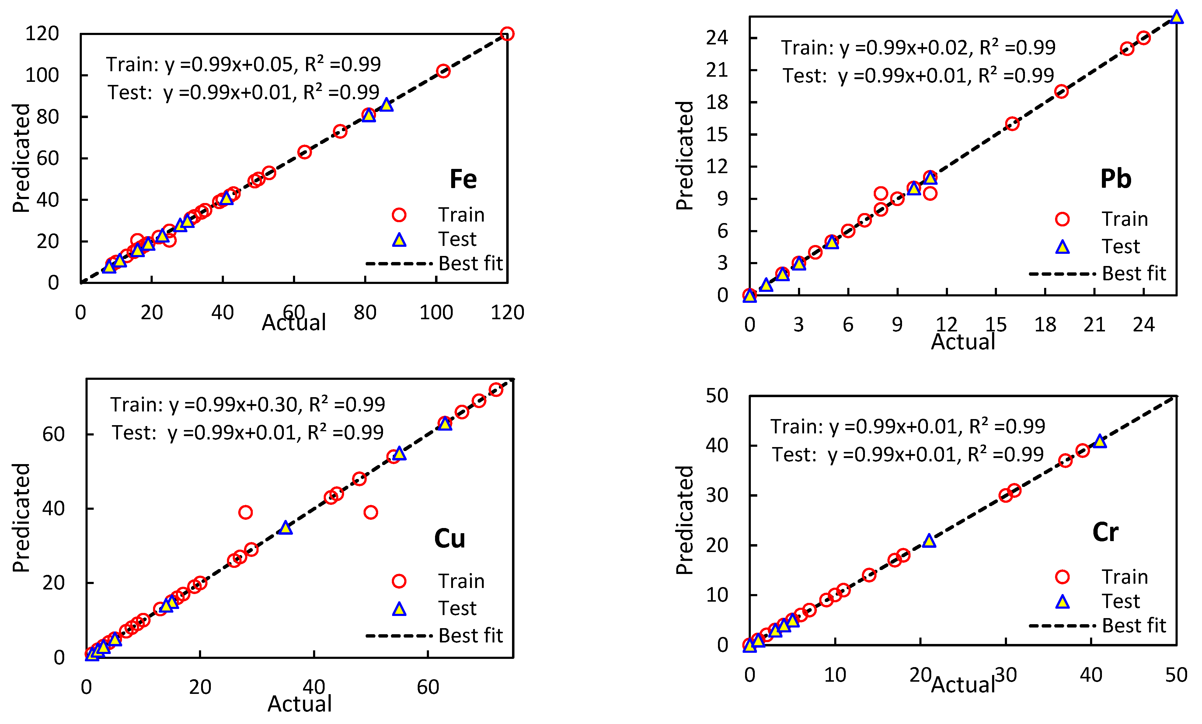
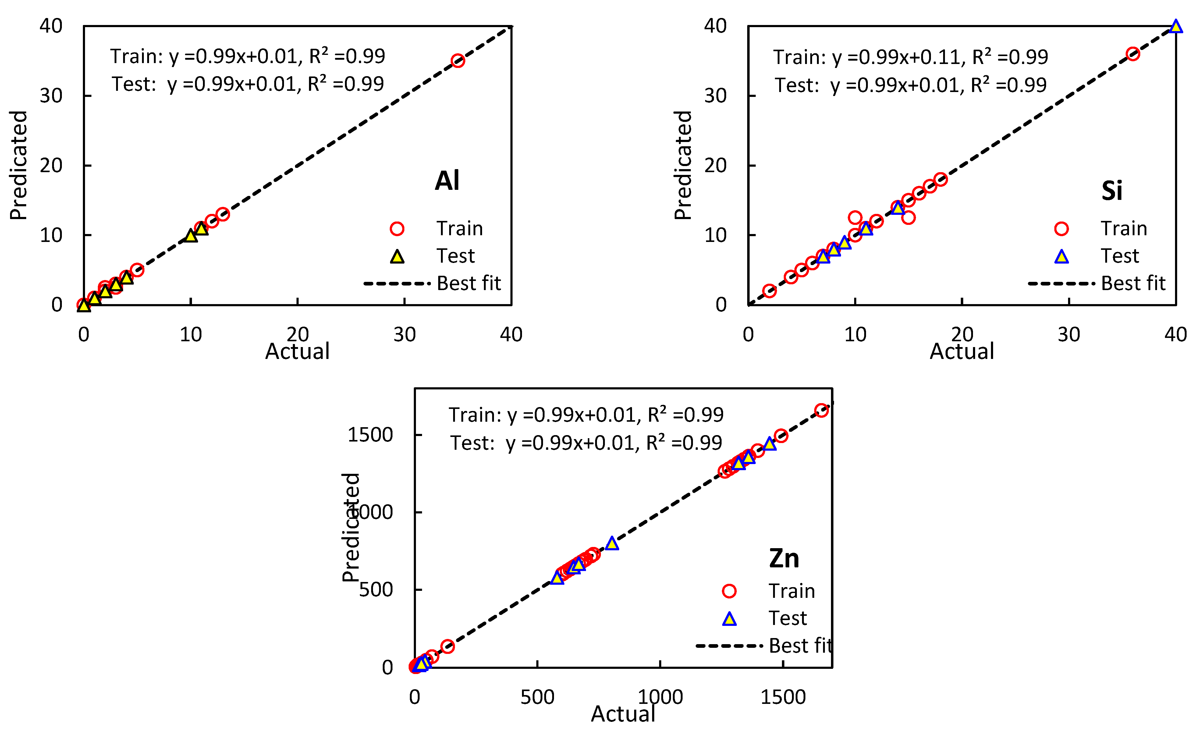
As mentioned earlier, this work is aimed to compare soft computing models performance in predicting the chemical properties (Fe, Pb, Cu, Cr, Al, Si, Zn) of lubricants based on their electrical properties (ε′, ε″, tan δ). Considering the statistical results of the models, the RBF exhibited the best performance. So, in this section, RBF parameters are discussed to promote its performance. Figure 4 shows the RBF efficiency (EF) in different hidden sizes for various chemical properties (Fe, Pb, Cu, Cr, Al, Si, Zn) at train and test steps. For example, if the hidden size is set to 12, the efficiency is the highest with no notable difference between the efficiency at train and test steps in “Fe” prediction. Figure 5 illustrates the RBF efficiency (EF) when employing different training algorithms for various chemical properties (Fe, Pb, Cu, Cr, Al, Si, Zn) at train and test steps. The "Trainlm" provided approximately the best RBF efficiency to predict all chemical properties (Fe, Pb, Cu, Cr, Al, Si, Zn) at train and test steps. Figure 6 plotted the coefficient of determination (R2) between the actual and predicted values of the spectral analysis indices of the lubricant. The coefficient is reported separately for the testing and training stages. It is seen that the slope of the regression line between the actual and predicted values in the RBF model is close to one and the intercept is very close to zero. Thus, the RBF model could predict the values of most spectral analysis indices of engine lubricant by a coefficient of 0.99.

3.2.2. Sensitivity Analysis

The ability of soft computing models to predict the chemical properties (Fe, Pb, Cu, Cr, Al, Si, Zn) of lubricants through electrical properties (ε′, ε″, tan δ) was investigated step by step as follow.
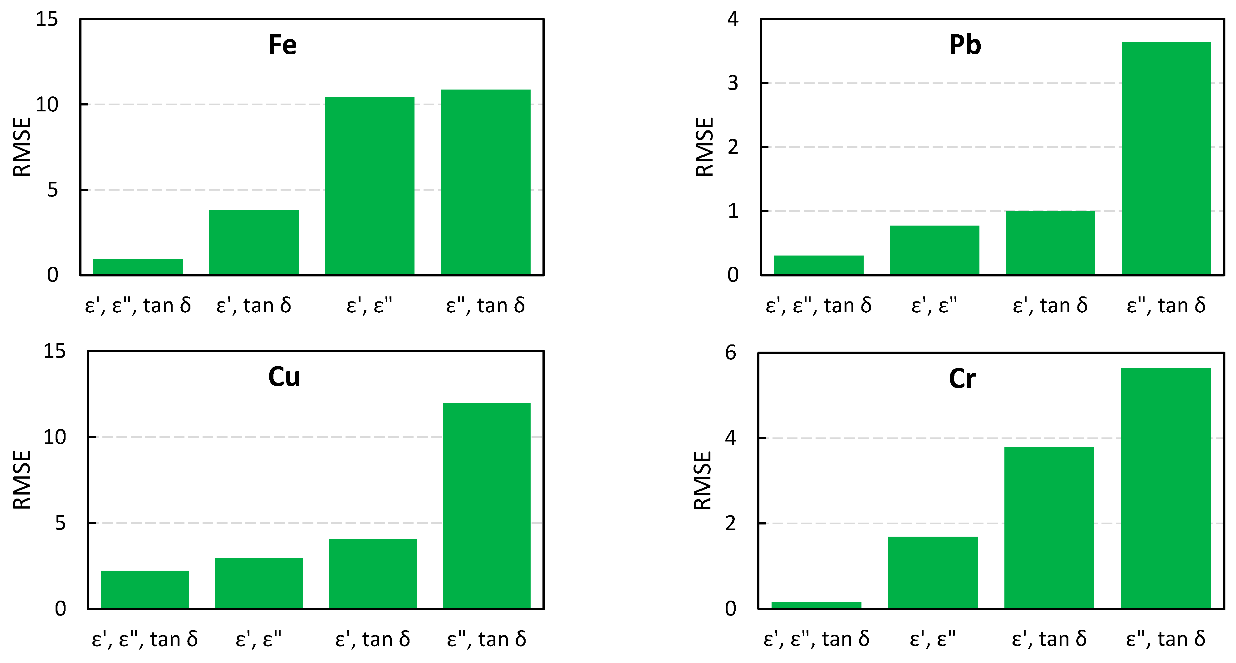
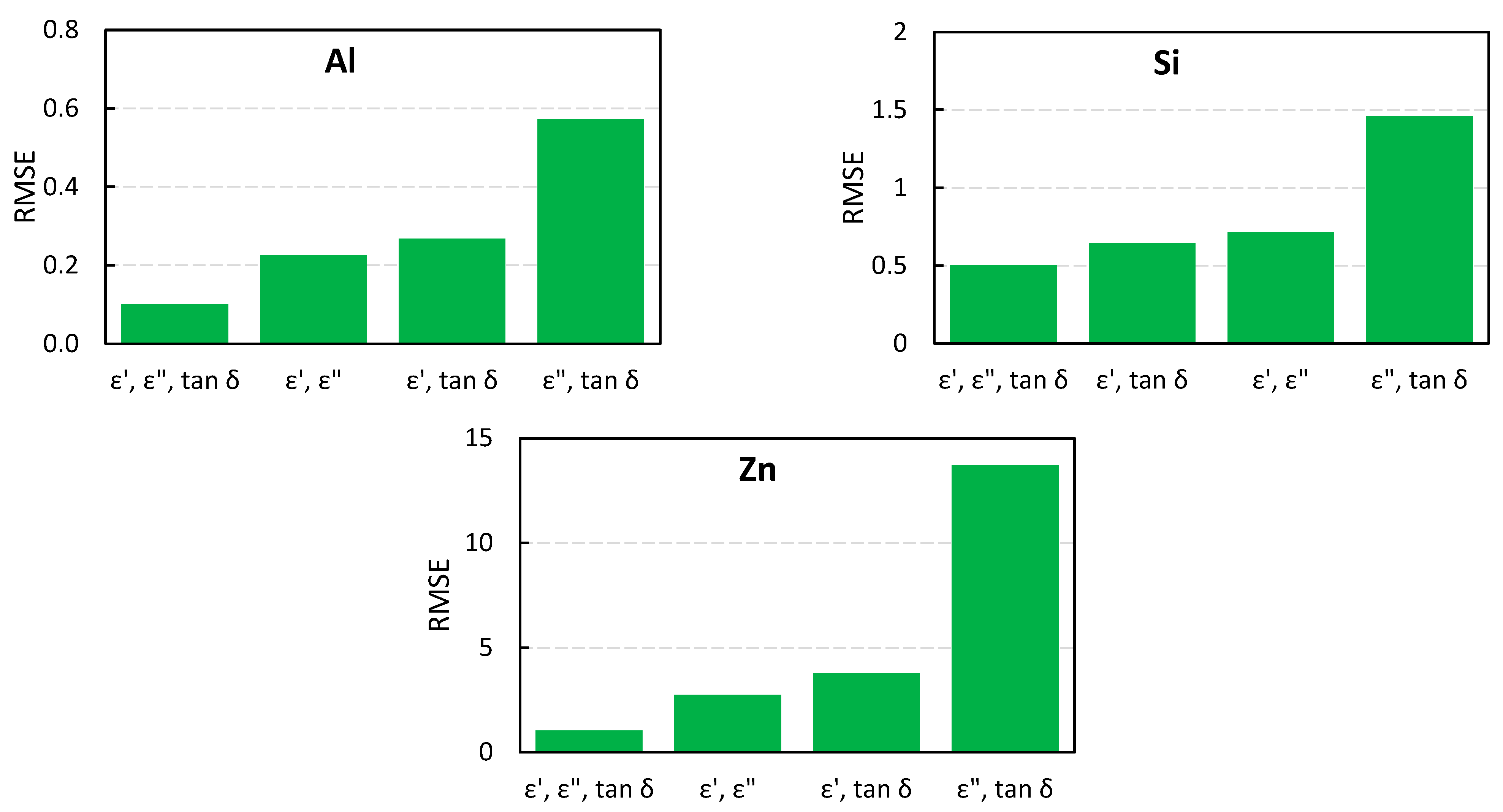
In Section 3.2, the performance of the models was evaluated, and the appropriate model (RBF) was reported. In Section 3.2.1, RBF parameters were set, and then sensitivity analysis was performed as an essential part to have a comprehensive study. In this section, the results of the sensitivity analysis are presented which are illustrated in Figure 7. The sensitivity analysis prioritizes the model inputs. For instance, if ε′ is removed from inputs, the RMSE is greatly increased in all terms. Since decreasing RMSE indicates that the model is more suitable, this means that ε′ is detected as a more effective input. In general, removing any of the inputs cannot improve the RMSE, so it is not recommended to remove any of the inputs.

4. Conclusion

This study focused on comparing the performance of soft computing models to predict the chemical properties (Fe, Pb, Cu, Cr, Al, Si, Zn) of engine lubricants through their electrical properties (ε′, ε″, tan δ). This can help to promote predictive maintenance. It is also an efficient method to promote academic efforts in terms of saving time, energy, and financial costs. In this work, the data was gained from two sources, consisting of data extracted from a published work and the data experimented during the current research. Subsequently, the RMSE and MAPE of the model’s performance were obtained for several frequency points. The RBF was the best model in predicting chemical properties (Fe, Pb, Cu, Cr, Al, Si, Zn) via electrical properties (ε′, ε″, tan δ) at 7.4 GHz frequency. The RBF parameters were then adjusted and optimized. For instance, in the RBF implemented to predict Al, the best hidden size and train algorithmic were 15 and ‘trainlm’, respectively. Finally, sensitivity analysis was implemented to prioritize the RBF inputs for each chemical property (Fe, Pb, Cu, Cr, Al, Si, Zn). The results showed that removing any of the inputs worsened the RMSE. In other words, none of the electrical attributes (ε′, ε″, tan δ) are recommended to be removed. It is concluded that soft computing models can promote condition monitoring of the lubricants through electrical properties (ε′, ε″, tan δ).

Acknowledgments

We thank the Ferdowsi University of Mashhad, Iran for funding the research project and also Tirage Company for making its maintenance database available.

Conflicts of Interest

The authors declare that there is no conflict of interest.

Abbreviations

ANN Artificial neural network MLP Multilayer perceptron
ANFIS Adaptive neuro-fuzzy inference system MLR Multiple Linear Regression
FL Fuzzy logic RFE Recursive feature elimination
GPR Gaussian process regression RBF Radial basic function
IAS Infrared absorption spectroscopy RMSE Root means square error
IS Impedance spectroscopy SVM Support vector machine
KNN K-nearest neighbor TDPQ Time depending on the particle quantifier
MAPE Mean absolute percentage error VNA Vector Network Analyzer

References

  1. Vališ, D.; Gajewski, J.; Žák, L. Potential for using the ANN-FIS meta-model approach to assess levels of particulate contamination in oil used in mechanical systems. Tribol. Int. 2019, 135, 324–334. [Google Scholar] [CrossRef]
  2. Upadhyay, R. Microscopic technique to determine various wear modes of used engine oil. J. Microsc. Ultrastruct. 2013, 1, 111–114. [Google Scholar] [CrossRef]
  3. Yan, R.; Gao, R. Complexity as a Measure for Machine Health Evaluation. IEEE Trans. Instrum. Meas. 2004, 53, 1327–1334. [Google Scholar] [CrossRef]
  4. Qiang, L., et al. Research on a Method for the Determination of Iron in Lubricating Oil. in 1st International Conference on Mechanical Engineering and Material Science (MEMS 2012). 2012. Atlantis Press.
  5. Avci, O.; Abdeljaber, O.; Kiranyaz, S.; Hussein, M.; Gabbouj, M.; Inman, D.J. A review of vibration-based damage detection in civil structures: From traditional methods to Machine Learning and Deep Learning applications. Mech. Syst. Signal Process. 2021, 147, 107077. [Google Scholar] [CrossRef]
  6. Zadhoush, M.; Nadooshan, A.A.; Afrand, M.; Ghafori, H. Constructal optimization of longitudinal and latitudinal rectangular fins used for cooling a plate under free convection by the intersection of asymptotes method. Int. J. Heat Mass Transf. 2017, 112, 441–453. [Google Scholar] [CrossRef]
  7. Kumbár, V.; Dostál, P. Oils degradation in agricultural machinery. Acta Universitatis Agriculturae et Silviculturae Mendelianae Brunensis 2013, 61, 1297–1303. [Google Scholar] [CrossRef]
  8. Alemayehu, B.; Kota, A.; Neidhard-Doll, A.; Chodavarapu, V.; Subramanyam, G. Cloud-connected real-time oil condition monitoring of utility transformers using impedance spectroscopy. Instrum. Sci. Technol. 2021, 49, 509–520. [Google Scholar] [CrossRef]
  9. Lazakis, I.; Raptodimos, Y.; Varelas, T. Predicting ship machinery system condition through analytical reliability tools and artificial neural networks. Ocean Eng. 2018, 152, 404–415. [Google Scholar] [CrossRef]
  10. Altıntaş, O.; Aksoy, M.; Ünal, E.; Akgöl, O.; Karaaslan, M. Artificial neural network approach for locomotive maintenance by monitoring dielectric properties of engine lubricant. Measurement 2019, 145, 678–686. [Google Scholar] [CrossRef]
  11. Pourramezan, M.-R.; Rohani, A.; Siavash, N.K.; Zarein, M. Evaluation of lubricant condition and engine health based on soft computing methods. Neural Comput. Appl. 2021, 34, 5465–5477. [Google Scholar] [CrossRef]
  12. Craft, J. Development of Interdigitated Electrode Sensors for Monitoring the Dielectric Properties of Lubricant Oils. 2010.
  13. Raadnui, S.; Kleesuwan, S. Low-cost condition monitoring sensor for used oil analysis. Wear 2005, 259, 1502–1506. [Google Scholar] [CrossRef]
  14. Grimmig, R.; Lindner, S.; Gillemot, P.; Winkler, M.; Witzleben, S. Analyses of used engine oils via atomic spectroscopy – Influence of sample pre-treatment and machine learning for engine type classification and lifetime assessment. Talanta 2021, 232, 122431. [Google Scholar] [CrossRef] [PubMed]
  15. Macin, V.; Tormos, B.; Sala, A.; Ramirez, J. Fuzzy logic-based expert system for diesel engine oil analysis diagnosis. Insight-Non-Destructive Testing and Condition Monitoring 2006, 48, 462–469. [Google Scholar] [CrossRef]
  16. Aghilinategh, N.; Nankali, S.; Babaei, M. Applying capacitance/inductance measurements for characterizing oil debris and pH. Indian J. Sci. Technol. 2016, 9. [Google Scholar] [CrossRef]
  17. Król, A.; Gocman, K.; Giemza, B. Neural networks as a tool to characterise oil state after porous bearings prolonged tests. Mater. Sci. 2015, 21, 466–472. [Google Scholar] [CrossRef]
  18. Li, L., et al. An identification and prediction model of wear-out fault based on oil monitoring data using PSO-SVM method. in 2017 Annual Reliability and Maintainability Symposium (RAMS). 2017. IEEE.
  19. RodRigues, J.; Costa, I.; Farinha, J.; Mendes, M.; Margalho, L. Predicting motor oil condition using artificial neural networks and principal component analysis. Eksploat. i Niezawodn. 2020, 22, 440–448. [Google Scholar] [CrossRef]
  20. Barsoukov, E. and J.R. Macdonald, Impedance spectroscopy theory, experiment, and. Applications, 2nd ed.(Hoboken, NJ: John Wiley &Sons, Inc., 2005), 2005.
  21. Heidari, P.; Rezaei, M.; Rohani, A. Soft computing-based approach on prediction promising pistachio seedling base on leaf characteristics. Sci. Hortic. 2020, 274, 109647. [Google Scholar] [CrossRef]
  22. Rezaei, M.; Rohani, A.; Heidari, P.; Lawson, S. Using soft computing and leaf dimensions to determine sex in immature Pistacia vera genotypes. Measurement 2021, 174, 108988. [Google Scholar] [CrossRef]
  23. Blanco, A.; Pino-Mejías, R.; Lara, J.; Rayo, S. Credit scoring models for the microfinance industry using neural networks: Evidence from Peru. Expert Syst. Appl. 2013, 40, 356–364. [Google Scholar] [CrossRef]
  24. Borghi, P.H.; Zakordonets, O.; Teixeira, J.P. A COVID-19 time series forecasting model based on MLP ANN. Procedia Comput. Sci. 2021, 181, 940–947. [Google Scholar] [CrossRef]
  25. Bazrafshan, O.; Ehteram, M.; Latif, S.D.; Huang, Y.F.; Teo, F.Y.; Ahmed, A.N.; El-Shafie, A. Predicting crop yields using a new robust Bayesian averaging model based on multiple hybrid ANFIS and MLP models. Ain Shams Eng. J. 2022, 13, 101724. [Google Scholar] [CrossRef]
  26. Sada, S.; Ikpeseni, S. Evaluation of ANN and ANFIS modeling ability in the prediction of AISI 1050 steel machining performance. Heliyon 2021, 7, e06136. [Google Scholar] [CrossRef] [PubMed]
  27. Vasileva-Stojanovska, T.; Vasileva, M.; Malinovski, T.; Trajkovik, V. An ANFIS model of quality of experience prediction in education. Appl. Soft Comput. 2015, 34, 129–138. [Google Scholar] [CrossRef]
  28. Stojčić, M.; Stjepanović, A.; Stjepanović, Đ. ANFIS model for the prediction of generated electricity of photovoltaic modules. Decis. Mak. Appl. Manag. Eng. 2019, 2, 35–48. [Google Scholar] [CrossRef]
  29. Chen, Y. and Y. Zhao. Face recognition using DCT and hierarchical RBF model. in International Conference on Intelligent Data Engineering and Automated Learning. 2006. Springer.
  30. Park, J.-W.; Venayagamoorthy, G.; Harley, R. MLP/RBF neural-networks-based online global model identification of synchronous generator. IEEE Trans. Ind. Electron. 2005, 52, 1685–1695. [Google Scholar] [CrossRef]
  31. Soleymani, S.A.; Goudarzi, S.; Anisi, M.H.; Hassan, W.H.; Idris, M.Y.I.; Shamshirband, S.; Noor, N.M.; Ahmedy, I. A novel method to water level prediction using RBF and FFA. Water Resour. Manag. 2016, 30, 3265–3283. [Google Scholar] [CrossRef]
  32. Otchere, D.A.; Ganat, T.O.A.; Gholami, R.; Ridha, S. Application of supervised machine learning paradigms in the prediction of petroleum reservoir properties: Comparative analysis of ANN and SVM models. J. Pet. Sci. Eng. 2020, 200, 108182. [Google Scholar] [CrossRef]
  33. Li, X.; Lord, D.; Zhang, Y.; Xie, Y. Predicting motor vehicle crashes using support vector machine models. Accid. Anal. Prev. 2008, 40, 1611–1618. [Google Scholar] [CrossRef]
  34. Ghorbani, M.A.; Zadeh, H.A.; Isazadeh, M.; Terzi, O. A comparative study of artificial neural network (MLP, RBF) and support vector machine models for river flow prediction. Environ. Earth Sci. 2016, 75, 1–14. [Google Scholar] [CrossRef]
  35. Zhang, Y.; Yang, H.; Cui, H.; Chen, Q. Comparison of the ability of ARIMA, WNN and SVM models for drought forecasting in the Sanjiang Plain, China. Nat. Resour. Res. 2020, 29, 1447–1464. [Google Scholar] [CrossRef]
  36. Cheng, M.-Y.; Huang, C.-C.; Van Roy, A.F. Predicting project success in construction using an evolutionary Gaussian process inference model. J. Civ. Eng. Manag. 2013, 19 (Suppl. 1), S202–S211. [Google Scholar] [CrossRef]
  37. Ghanizadeh, A.R.; Heidarabadizadeh, N.; Heravi, F. Gaussian process regression (Gpr) for auto-estimation of resilient modulus of stabilized base materials. Journal of Soft Computing in Civil Engineering 2021, 5, 80–94. [Google Scholar]
  38. Schulz, E.; Speekenbrink, M.; Krause, A. A tutorial on Gaussian process regression: Modelling, exploring, and exploiting functions. J. Math. Psychol. 2018, 85, 1–16. [Google Scholar] [CrossRef]
  39. Quinonero-Candela, J.; Rasmussen, C.E. A unifying view of sparse approximate Gaussian process regression. The Journal of Machine Learning Research 2005, 6, 1939–1959. [Google Scholar]
  40. Arvanitidis, A.I.; Bargiotas, D.; Daskalopulu, A.; Kontogiannis, D.; Panapakidis, I.P.; Tsoukalas, L.H. Clustering Informed MLP Models for Fast and Accurate Short-Term Load Forecasting. Energies 2022, 15, 1295. [Google Scholar] [CrossRef]
  41. Thapa, S.; Zhao, Z.; Li, B.; Lu, L.; Fu, D.; Shi, X.; Tang, B.; Qi, H. Snowmelt-driven streamflow prediction using machine learning techniques (LSTM, NARX, GPR, and SVR). Water 2020, 12, 1734. [Google Scholar] [CrossRef]
  42. Okwu, M.; Adetunji, O. A comparative study of artificial neural network (ANN) and adaptive neuro-fuzzy inference system (ANFIS) models in distribution system with nondeterministic inputs. Int. J. Eng. Bus. Manag. 2018, 10. [Google Scholar] [CrossRef]
  43. Slama, S., A. Errachdi, and M. Benrejeb. Model reference adaptive control for MIMO nonlinear systems using RBF neural networks. in 2018 international conference on advanced systems and electric technologies (IC_ASET). 2018. IEEE.
  44. Tabari, H.; Kisi, O.; Ezani, A.; Talaee, P.H. SVM, ANFIS, regression and climate based models for reference evapotranspiration modeling using limited climatic data in a semi-arid highland environment. J. Hydrol. 2012, 444-445, 78–89. [Google Scholar] [CrossRef]
  45. Taki, M.; Ajabshirchi, Y.; Ranjbar, S.F.; Rohani, A.; Matloobi, M. Modeling and experimental validation of heat transfer and energy consumption in an innovative greenhouse structure. Inf. Process. Agric. 2016, 3, 157–174. [Google Scholar] [CrossRef]
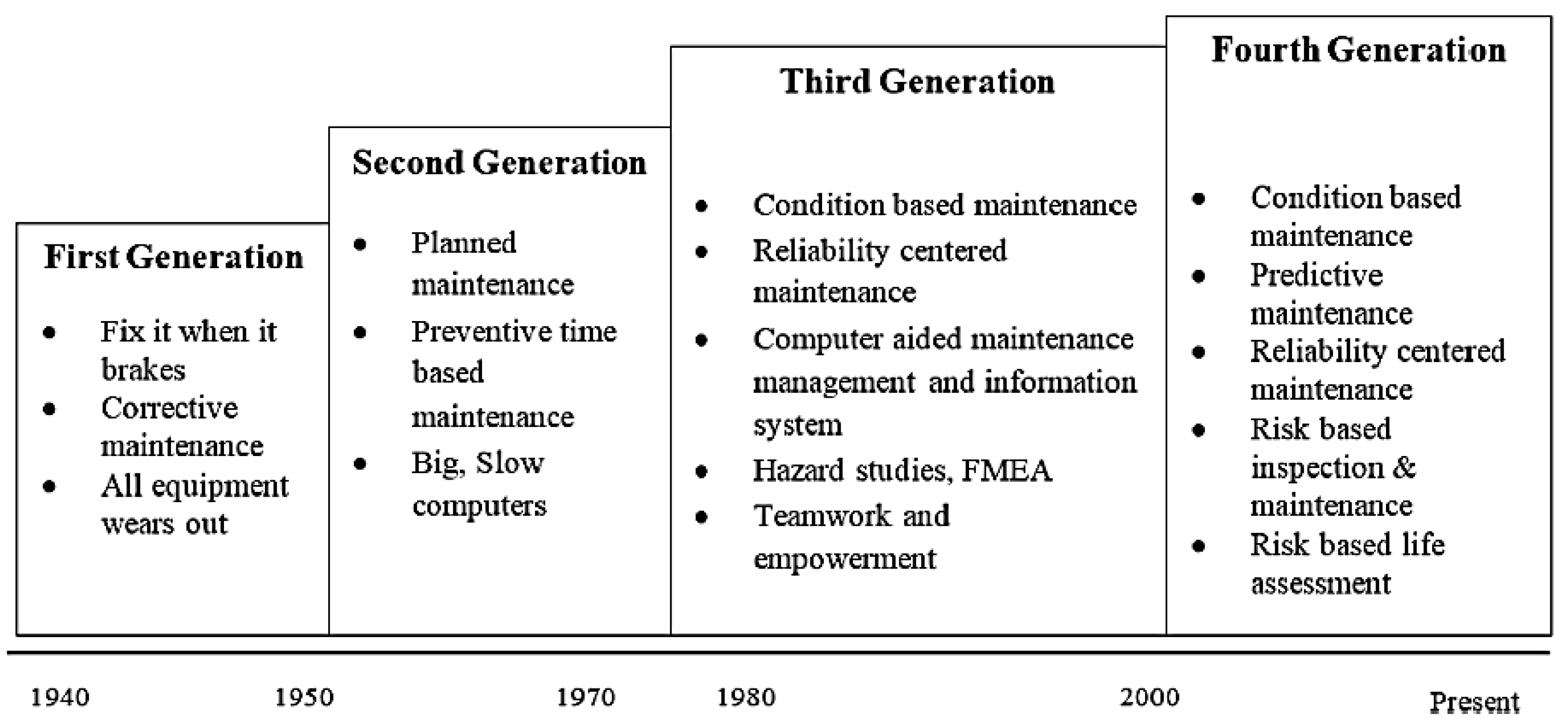
Figure 1. Development of maintenance strategies [9].
Preprints 69740 g001
Figure 2. The schematic view of dataset preparation from sources.
Preprints 69740 g002
Figure 3. The experimental setup and its schematic view for measuring dielectric properties of lubricants.
Preprints 69740 g003
Figure 4. Result of RBF efficiency in different hidden sizes for various chemical properties.
Preprints 69740 g004aPreprints 69740 g004b
Figure 5. Result of RBF efficiency in different train algorithms for various chemical properties.
Preprints 69740 g005aPreprints 69740 g005b
Figure 6. Actual and predicted values of the chemical properties in two steps (training and testing).
Preprints 69740 g006aPreprints 69740 g006b
Figure 7. Result of sensitivity analysis to prioritize RBF inputs for various chemical properties.
Preprints 69740 g007aPreprints 69740 g007b
Table 1. Spectral analysis results for the samples provided by Tirage company (Unit: ppm).
Sample No. Fe Pb Cu Cr Al Si Zn
1 11.05 2.83 0.98 1.26 3.62 8.79 1319
2 9.94 0 0.97 0.46 1.61 17.77 1362
3 30.25 0 1.64 5.33 10.18 9.23 1359
4 81.17 0 2.59 7.46 34.59 36.21 1493
5 13.19 1.8 0.59 1.8 1.09 7.14 1281
6 24.65 0 1.25 1.55 5.05 9.89 1398
7 9.24 0 0.92 0.11 1 6.11 1362
8 15.46 0 1.75 0 0.38 4.01 1360
9 39 4.42 7.78 6.52 10.93 16.29 1297
10 39.76 3.2 1.4 2.2 3.77 15.44 1657
11 34.69 0.18 1.23 7.2 13.45 16.55 1264
12 39.67 3.91 2.31 6.48 12.45 16.33 1342
13 86.06 1.17 2.76 3.69 10.95 40.05 1445
14 21.73 3.22 7.23 0.91 5.31 7.27 1317
15 8.17 1.79 3.23 0.04 0 7.22 803
16 49.75 3.51 4.11 4.15 5.07 13.65 1327
Table 2. Dielectric properties measurement results for samples provide by Tirage Company.
Sample No. 2.40 GHz 5.80 GHz 7.40 GHz
ε′ ε″ tan δ ε′ ε″ tan δ ε′ ε″ tan δ
1 2.62 0.15 0.058 2.94 0.13 0.044 2.55 0.23 0.090
2 2.68 0.12 0.045 2.99 0.10 0.033 2.60 0.18 0.069
3 2.45 0.09 0.037 2.79 0.07 0.025 2.40 0.17 0.071
4 2.55 0.05 0.020 2.86 0.05 0.017 2.47 0.12 0.049
5 2.60 0.13 0.051 2.91 0.12 0.041 2.52 0.21 0.083
6 2.58 0.13 0.051 2.90 0.11 0.038 2.50 0.20 0.080
7 2.60 0.17 0.066 2.93 0.14 0.048 2.52 0.26 0.103
8 2.54 0.20 0.079 2.85 0.19 0.067 2.43 0.30 0.123
9 2.53 0.08 0.032 2.83 0.06 0.021 2.45 0.15 0.061
10 2.52 0.06 0.025 2.81 0.05 0.018 2.43 0.13 0.053
11 2.55 0.09 0.036 2.88 0.07 0.024 2.50 0.14 0.056
12 2.50 0.07 0.029 2.79 0.05 0.018 2.42 0.14 0.058
13 2.41 0.05 0.021 2.70 0.04 0.015 2.34 0.10 0.043
14 2.66 0.11 0.042 2.97 0.10 0.034 2.58 0.16 0.062
15 2.60 0.13 0.051 2.93 0.12 0.041 2.53 0.21 0.083
16 2.50 0.07 0.029 2.81 0.06 0.021 2.42 0.13 0.054
Table 3. Result of correlations between variable 1 (chemical properties) and variable 2 (electrical properties).
Var. 1 Var. 2 Corr. Var. 1 Var. 2 Corr. Var. 1 Var. 2 Corr. Var. 1 Var. 2 Corr.
Fe ε′ -0.13ns Cu ε′ 0.45** Al ε′ -0.23 *** Zn ε′ -0.54**
ε″ -0.20*** ε″ 0.53** ε″ -0.49** ε″ -0.77**
tan δ -0.22*** tan δ 0.53** tan δ -0.56** tan δ -0.79**
Pb ε′ 0.41** Cr ε′ 0.45** Si ε′ -0.14 ns
ε″ 0.48** ε″ 0.45** ε″ -0.42**
tan δ 0.48** tan δ 0.41** tan δ -0.50**
Table 4. Comparing the performance of models by RMSE and MAPE.
Frequency 2.4 GHz 5.80 GHz 7.40 GHz
ML model RBF MLP ANFIS GPR SVM RBF MLP ANFIS GPR SVM RBF MLP ANFIS GPR SVM
Fe RMSE 2.4 11.0 2.4 16.8 23.4 1.4 23.9 1.5 19.7 17.3 0.9 15.5 0.9 14.3 16.5
MAPE 3.7 33.8 3.8 48.5 51.9 2.8 69.5 2.6 34.5 43.5 0.9 47.3 1.1 40.3 36.2
Pb RMSE 1.4 5.4 2.2 3.8 15.6 1.0 4.9 1.0 5.3 6.5 0.3 3.3 0.3 5.5 7.5
MAPE - - - - - - - - - - - - - - -
Cu RMSE 4.4 22.4 5.0 16.4 19.0 3.9 18.7 3.9 18.6 53.2 2.2 13.2 2.2 18.5 21.3
MAPE 10.3 70.0 10.2 70.7 68.3 7.9 40.3 9.3 93.4 87.2 1.3 11.0 2.4 96.8 72.3
Cr RMSE 4.0 13.3 4.3 12.7 15.7 3.9 13.2 8.1 12.7 15.5 0.2 13.2 3.5 11.3 16.2
MAPE - - - - - - - - - - - - - - -
Al RMSE 0.7 0.7 0.8 0.7 0.9 0.2 0.7 0.3 0.7 3.5 0.1 0.7 0.1 0.7 0.9
MAPE - - - - - - - - - - - - - - -
Si RMSE 0.7 3.4 2.2 2.5 4.3 0.6 2.9 0.8 3.1 3.5 0.4 2.2 0.5 2.9 3.3
MAPE 4.3 38.4 8.9 28.1 48.2 1.7 28.2 1.9 33.0 36.1 0.7 25.7 1.1 24.4 34.2
Zn RMSE 10.3 20.7 80.3 29.2 39.1 6.5 41.9 53.8 28.0 28.3 1.0 6.7 2.2 28.6 35.3
MAPE 16.4 32.0 70.7 35.3 48.3 9.0 80.9 74.9 75.2 65.4 1.4 25.4 2.3 73.1 65.4
Disclaimer/Publisher’s Note: The statements, opinions and data contained in all publications are solely those of the individual author(s) and contributor(s) and not of MDPI and/or the editor(s). MDPI and/or the editor(s) disclaim responsibility for any injury to people or property resulting from any ideas, methods, instructions or products referred to in the content.
Copyright: This open access article is published under a Creative Commons CC BY 4.0 license, which permit the free download, distribution, and reuse, provided that the author and preprint are cited in any reuse.
Prerpints.org logo

Preprints.org is a free preprint server supported by MDPI in Basel, Switzerland.

Subscribe

© 2024 MDPI (Basel, Switzerland) unless otherwise stated