
Submitted:
07 March 2023
Posted:
08 March 2023
You are already at the latest version
Abstract
This article presents the results of the consideration of the Bertrand paradox in terms of geometric probability theory. Although the method and conclusions of this article are straightforward, no equivalent studies were found when reviewing the relevant literature. This could be conditioned by the fact that the hypotheses presented in this research have low intuitive obviousness and, in contrast, could be due to the historically established agreement regarding the issue. This article shows that out of three classical solutions to the problem described by Bertrand, two methods are inconsistent with the claimed relative objectivity. Although the remaining solution (1/4) seems to be the most correct, we cannot claim that we have exhaustively ruled out all aspects that could reduce its adequacy to solve the problem.
Keywords:
Bertrand paradox
; geometric probability
; probability estimation method
MSC:
1. Introduction
The Bertrand paradox is a problem based in probability theory that was formulated more than a century ago. It is one of the classic examples of how a change in the method of random choice for the same events could lead to various results of their probability. Since this paradox holds an important place in the history of development of geometric probability theory [1, 2], this problem is still used as a convenient example of how the results depend on the chosen method [3, 4].
There are three classical solutions to this paradox, and each of them has different results for the same problem. The paradox can be presented as follows: there is an equilateral triangle inscribed in a circle (for convenience, hereinafter we will refer to these as the triangle and as the main circle or circumference). The task is to define the probability that a random chord is longer than a side of the triangle inscribed in this circle.
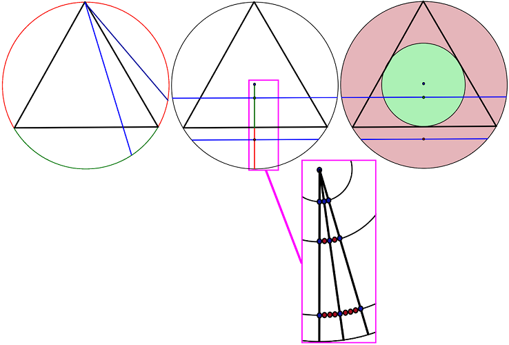
Three classical solutions considered in the article are based on different methods by which a chord is chosen at random (Picture 1).
The first solution is to consider all chords that can be constructed from a random point on the circle. If one assumes that this point is at one vertex, the chords that end on the arc between the endpoints of the triangle are longer than the side of the triangle, and all the others are not. Thus, the other chord endpoint could lie only within this 60 degrees out of 180 degrees to meet the condition. Assuming that the choice of an angle is random, the probability is 1/3.
Two other solutions are based on choosing a point that is the center of a chord, since it is possible to construct only one chord through each point except the central one.
According to one of these solutions, we need to choose a random radius that intersects the center of one of the triangle’s sides for convenience. Thus, all points that lay on this radius inside the triangle correspond to the chords that are longer than the side of the triangle; the rest are shorter. Since the side of the triangle bisects the radius, with a random choice of a point on the radius, the probability is 1/2.
The third method is based on random choosing of a chord’s center inside the circle. Thus, all points that fall within the inscribed circle correspond to the chords that are longer than the side of the triangle. The rest are shorter. Since the radius of the main circle is twice the radius of the inscribed one, their areas are 4:1. So, with a random choice of a point inside the circle, the probability that it falls within the inscribed circle is 1/4.
Figure 1.
Three classical solutions: 1/3, 1/2, and 1/4.
Thus, the results of probability depend on the method of random selection we choose. This article considers only these three classical solutions presented by Bertrand. Since the proposed method of consideration is quite simple, in order to eliminate unnecessary complication, we will restrict ourselves to a textual description without using formulas.
These methods are largely objective and, in general, have equal validity. Nevertheless, many authors consider the second method (1/2) to be more accurate in terms of meeting the required results [5]. In addition, if we take into account that the center of the circle defines multiple variants of chords, none of these methods seems to be ideal [6]. Further, for our convenience, we will not take into account the central point at all, since it is not crucial for our method of analysis. These two issues will be addressed at the end of the article.
2. Comparison of the Second and Third methods
The second method (1/2) implies a certain assumption that is controversial in terms of maximum invariance. More importantly, it could lead to a contradiction with the third method (1/4), which does not allow them to be considered as mutually alternative. The point of this assumption is that we consider equal distribution of the probability of choosing a random point along the entire radius. This means that there are an equal number of possible random centers of circle chords throughout the length of the radius. Only in this case, the choice of one of the possible radiuses, as a standard of the probability estimation, allows us to assess the overall probability of choosing a random chord. That is, the number of possible random points is the same at any distance from the midpoint of the circle.
At the same time, this assumption means that the number of possible random points on any random smaller circle in the area between the midpoint and the edge of the main circle is equal. Therefore, regardless of the circumference, the number of points is equal. The second method (1/2) can be considered as a solution to the problem only by taking into account this assumption.
On the whole, such an assumption can be justified, since if we consider an infinite number of radiuses that intersect all the given circles, then the number of points on these circles intersected by the radiuses is also equal. With this assumption, the displacement of the radius along the points of the larger of two arbitrary circles will lead to the displacement between the points on the smaller one.
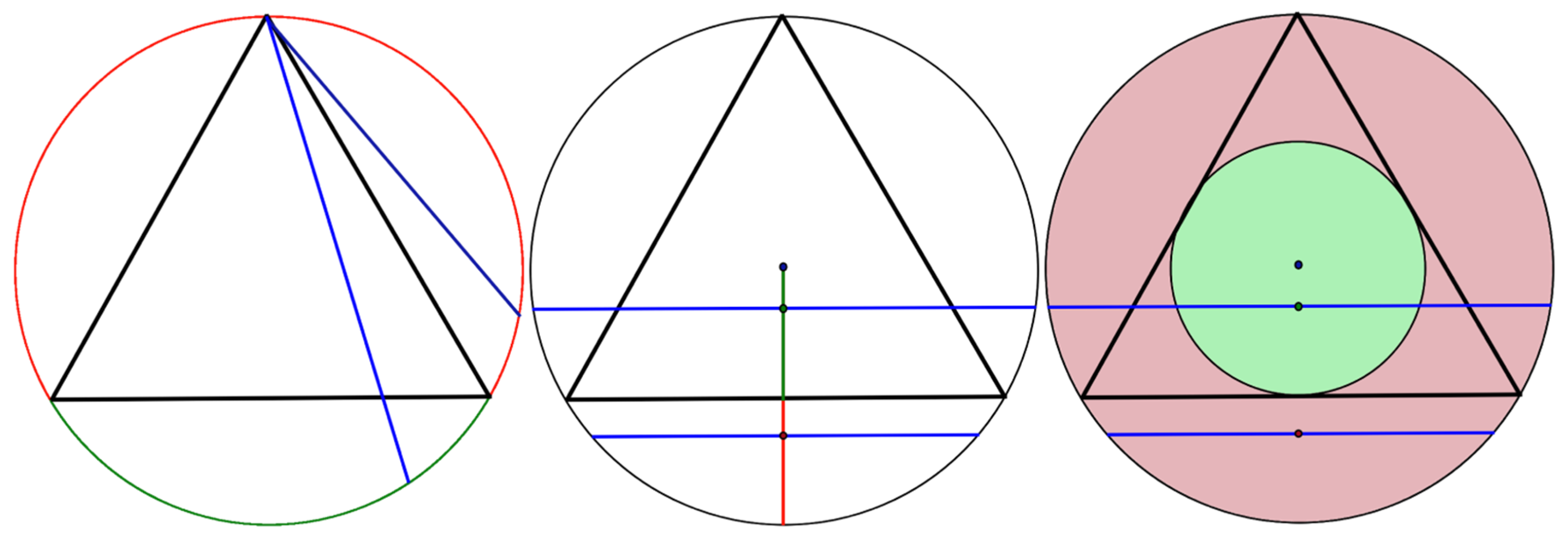
Similarly, two circles inscribed in a cone could be considered (Figure 2). Let us take a ray from the vertex of a cone that intersects both circles. If we displace the ray along the points of the larger circle, it will cause the displacement between the points of the smaller one. Thus, the number of such points is equal inside both circles. Now let us assume that the radiuses of the circles have a ratio of 1:2 and place both circles on a plane, with their centers aligned. Now let us estimate the probability of a random point falling into the smaller circle and into the remaining area of the larger circle. The probability of falling into the larger circle that is outside of the smaller one is equal to the number of points in the larger circle minus the number of points in the smaller one. Since these numbers are equal, the possibility of falling outside of the smaller circle is zero. Therefore, all randomly chosen points will be in the smaller circle.
Thus, making an analogy between the second and the third method to solve the Bertrand paradox, in the third solution we achieve 100% instead of 1/4. Obviously, this cannot be considered as a correct solution, though we took into account the assumption on which the second classic method for solving the problem is based. In the same way that our exaggerated formulation of the third method ignores all points outside the smaller circle, the second one ignores all additional points outside the smaller circle that appear when moving away from the center of the circle (Figure 3).
Hence, the second method (1/2) can be considered either as initially incorrect or as not being an alternative to the third solution (1/4), while also being correct only for a more specific problem than the one that was formulated by Bertrand.
As was mentioned above, the main issue of the formulation that limits its application is that the number of points on each arbitrary circle, both around the center of the circle and at its border, is the same, regardless of the circumference. This shortcoming could be eliminated by introducing additional points on the circles that are close to the edge of the circle. In fact, this will provide the third solution to the problem. It is worth noting that the dependence of the number of points on the circle on its circumference in the context of the Bertrand paradox is addressed by D. Rizza [7], although this concept was not applied to compare the results of two solutions.
A similar misrepresentation of the original assumptions can be found while considering another Bertrand problem described in the same work. The question is to evaluate the probability that a number randomly chosen from 0 to 100 [8] is greater than 50. Although the intuitively obvious answer is 1/2, Bertrand provides another solution with a different result. Following the statement that each number corresponds to its square, Bertrand chooses a random number out of 10,000 (which is 100 squared) and then calculates its root. Since the numbers greater than 50 correspond to the squared numbers greater than 2500, the probability of favorable cases is 3/4. We can also use cubed numbers or any exponent instead of square numbers.
When considering that solution, it is obvious that in the case of the squared numbers whose roots correspond to the integers in the range from 0 to 100, there are exactly 100 such squared numbers in the range from 0 to 10,000 [9]. Therefore, the probabilities are actually equal. However, at the same time, as the number increases towards 100, the difference between the squares of consecutive numbers also increases. Thus, if the probabilities of integers from 0 to 100 are estimated by choosing integers between 0 and 10,000 and rounding their roots to integers, then the randomness of the final choice will be distorted. This occurs due to the adding of extra options to the sample while going from 0 to 100. It will be distorted in the same way by any fractional division of any one or both ranges of numbers, that is, from 0 to 100 and from 0 to 10,000.
Thus, a strong analogue can be drawn between large numbers that are close to 100 and large circles that are close to the border of the main circle. The only difference is that these two solutions are completely inverted in terms of distortion. In the case with the chords placed on a plane, the solution is distorted by reducing it to a linear problem, and in the case of number choosing, on the contrary, the linear problem is distorted by exponentiation. We can assume that both problems were described in the same work one after another due to the similarity of their errors.
3. First method
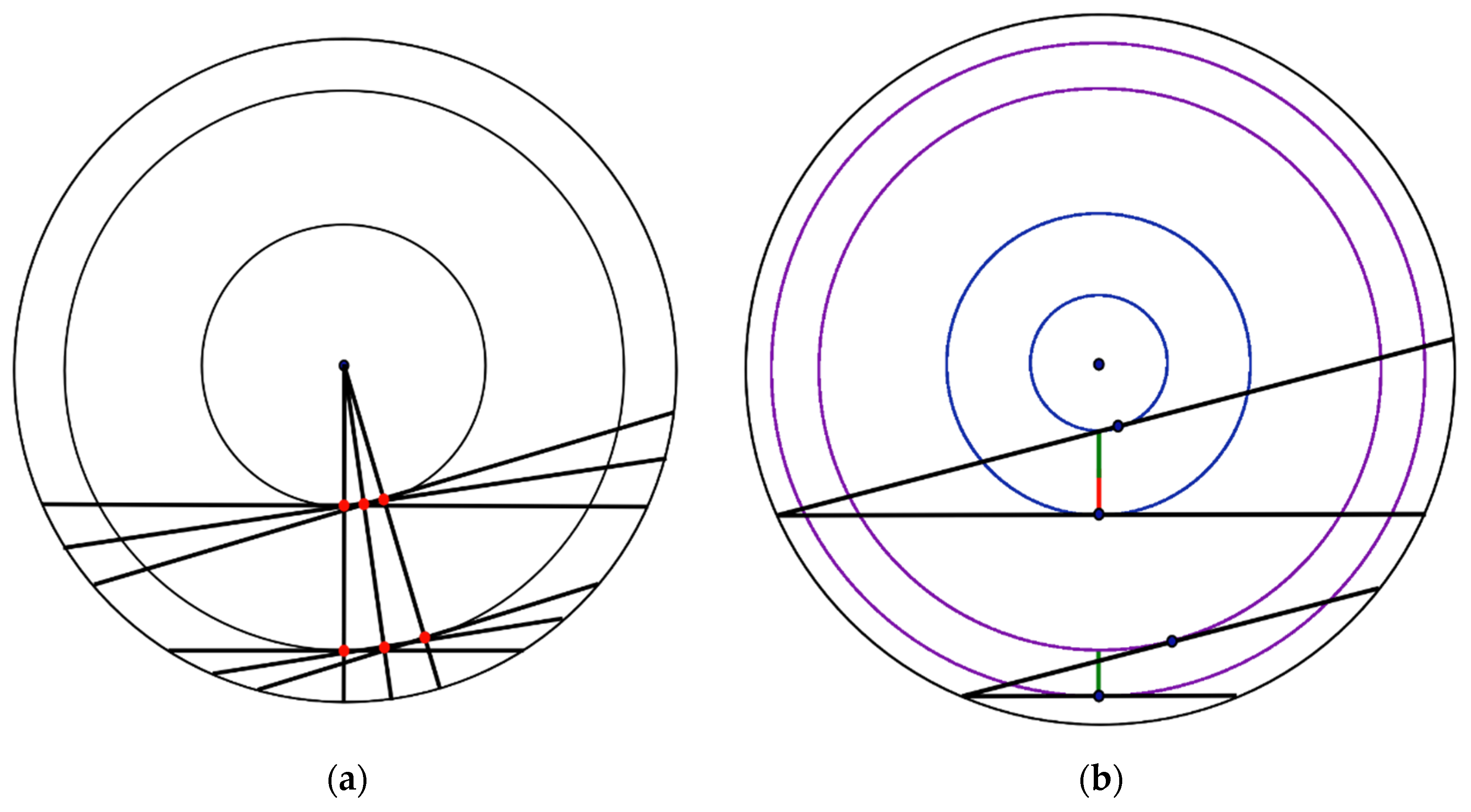
The first method, which provides 1/3 as the solution, is fundamentally different from the two others. In this case, a random choice of a chord is made by a random choice of one of its points while the second point is fixed, but not through the point of its center. That is, the number of possible chords is equal to the number of points on a circle, except for the first arbitrarily chosen point. That number of chords is located within the 180 degree range relative to this fist arbitrary point. Thus, the possibility that the chords are longer than a side of the triangle is described as a ratio of two ranges, the common 180 degree arc and the smaller one with a measure of 60 degrees, which includes the longer chords. Thus, all arbitrary points on the circle are taken as equivalent in terms of choosing them as the second point to the first one chosen (Figure 4a). Such assumed equality of all points, which could be used to construct a set of chords, allows us to estimate the probability using just one arbitrarily chosen point.
However, if we examine this solution closely, the last assumption is not true for the same reason as in the case when the probability is 1/2. Let us consider an arbitrary displacement along the circumference of both endpoints of a chord by equal distance and in the same direction. This will also displace the center of this chord along a conditional inscribed circle, which is the smaller one. The closer the chord is to the diameter, the closer such a conditional inscribed circle is to the center of the main circle, and vice versa. Along with this, there is the same number of possible displacements for each pair of points that are endpoints of an arbitrary chord. Thus, the considered solution to the problem also proceeds from the premise that the numbers of points on the circles are equal, regardless of their length. For this reason, this solution cannot be considered as an alternative to the third one (1/4).
However, if we consider the first two solutions (1/2 and 1/3), the formulation of which inevitably assumes the same premise, then it is logical to expect that they will give the same answer, which is not true. Let us consider what additional premise assumed in the formulation of the first solution (1/3) does not allow us to consider it as an alternative to the second solution (1/2).
Let us consider an arbitrary displacement of the end of the chord opposite to the fixed point (Figure 4b). The angle between a chord and the circle will differ significantly depending on the proximity to the diameter of a particular chord. Therefore, for such cases, the same displacement along the circumference will lead to a different distance between the center of a chord and the center of the circle. The chords that are closer to the edge of the circumference will move away from the center more slowly. This leads to a greater density of smaller conditional circles with centers of chords near the edge of the main circle. This can be seen as an assumption about a lower density of points near the center of the circle, which partially compensates for the assumption that the point density decreases on such small circles. Thus, the two assumptions inevitably implied in the solution partly reduce the effect of one another. This leads to an answer that is different from the solution when we use only one of the mentioned assumptions.
4. Discussion
We proved that, in terms of geometry, the first and second classical solutions to this problem (1/3 and 1/2) imply false assumptions concerning invariance. Bertrand, himself, when formulating the problem, adds the same phrase to the first (1/3) and to the second (1/2) solutions: "la symétrie du cercle ne permet d'y attacher aucune influence, favorable ou défavorable à l'arrivée de l'événement demandé" [10], which can be translated as “the symmetry of the circle does not allow any effect on the probability, either favorably or unfavorably”. Nevertheless, Bertrand twice creates a false perception of the truth of these solutions by using this particular phrase. Of course, the options 1/2 and 1/3 are not completely erroneous; there are likely situations where such a solution is acceptable. However, for the general case, they are incorrect.
The third method (1/4) has no obvious disadvantages in terms of geometry. However, as we mentioned at the beginning of the article, some scientists also criticize the formulation of the third method, claiming that all three solutions are formulated incorrectly due to the multivariance of the chords passing through the center. For similar reasons, due to the incorrectness of the formulation that concerns the part of diameters, it is often suggested that only the third solution (1/4) is incorrect [11]. Nevertheless, if we assume that the third method is more optimal in the part that concerns other chords, then it will probably remain so if we add any common condition regarding the consideration of diameters to all three solutions.
Modeling is often used to evaluate these three classical methods [12, 13]. According to the results, the first two methods have a high density of points and centers of chords in the center of the circle, whereas the third one (1/4) shows an even distribution of points. In addition, if we also construct the chords when building the model, for the first and the second solution, the circle will be more evenly filled with chords, which intuitively gives the impression of a more realistic random choice. For this reason, the second method (1/2) is proposed to be the most correct solution, since it gives the most even visual distribution of chords during the modeling. On this basis, there are also more rigorous formulations of the proof, based on the statement that if the chords are randomly distributed, then they must be uniformly distributed in any area of the circle [14]. However, such an intuitive perception is incorrect if we base it on the following argument. All chords with a midpoint close to the center of the circle also intersect the areas close to the edge of the circle, thereby “shading” them. However, chords with midpoints far from the center of the circle stretch only along the edges of the circle, without touching the center. Thus, even “shading” of all areas is impossible due to the invariant solution to the problem.
Therefore, it can be assumed that, in terms of geometry, there is one solution (1/4) to this problem, which is more consistent with the principle of indifference. Hence, it has obvious priority over the others, although it cannot be considered the only right solution to the Bertrand paradox. It should also be noted that if it is ultimately determined that one of the three Bertrand methods is the sole correct one, this will not diminish his contribution as the initiator of research and discussions. There is always a probability that Bertrand, himself, did not consider all three solutions to be the right ones.
References
- Calka P. Some Classical Problems in Random Geometry. Stochastic geometry, 2019, 2237, pp.1- 43, Lecture Notes in Mathematics, 978-3-030-13546-1. [CrossRef]
- Hug, D., Reitzner, M. Introduction to Stochastic Geometry. In: Peccati, G., Reitzner, M. (eds) Stochastic Analysis for Poisson Point Processes. Bocconi & Springer Series, 2016, vol 7. Springer, Cham. [CrossRef]
- Rocchi, P. and Burgin, M. An Essay on the Prerequisites for the Probability Theory. Advances in Pure Mathematics, 2020, 10, 685-698. [CrossRef]
- Jeffrey M.R. Uncertainty in classical systems (with a local, non-stochastic, non-chaotic origin) J. Phys. A: Math. Theor., 2020, 53 115701. 1088.
- Aerts, D., & de Bianchi, M. S. Solving the hard problem of Bertrand’s paradox. Journal of Mathematical Physics, 2014, 55(8), 083503. [CrossRef]
- Rowbottom, D. P. Bertrand's Paradox Revisited: Why Bertrand's ‘Solutions’ Are All Inapplicable. Philosophia Mathematica, 2013, 21(1), 110-114. [CrossRef]
- Rizza D. A Study of Mathematical Determination through Bertrand’s Paradox, Philosophia Mathematica, 2018, 26(3), 375–395. [CrossRef]
- Klyve, D. In Defense of Bertrand: The Non-Restrictiveness of Reasoning by Example. Philosophia Mathematica, 2013, 21(3), 365–370. [CrossRef]
- Petroni, N. C. Thou shalt not say" at random" in vain: Bertrand's paradox exposed. arXiv preprint 2018.
- Bertrand, Joseph, "Calcul des probabilités" [Calculation of probabilities], Gauthier-Villars, 1889, p. 4-5.
- Shackel, N. Bertrand’s Paradox and the Principle of Indifference. Philosophy of Science, 2007, 74, 150 – 175. [CrossRef]
- Jaynes, E. T. The Well-Posed Problem, Foundations of Physics, 1973, Т. 3: 477–493. [CrossRef]
- Marakis E., Velsink M. C., van Willenswaard L. J. C., Uppu R., Pinkse P. W. H. Phys. Rev., 2019, E 99, 043309.
- Wang J., Jackson R., Resolving Bertrand's probability paradox, Int. J. Open Probl. Comput. Sci. Math., 2011, 4 (3), 72–103.
Figure 2.
Two circles inscribed in a cone.
Figure 3.
Additional points that appear when moving away from the center of the circle with a displacement of radiuses.
Figure 3.
Additional points that appear when moving away from the center of the circle with a displacement of radiuses.
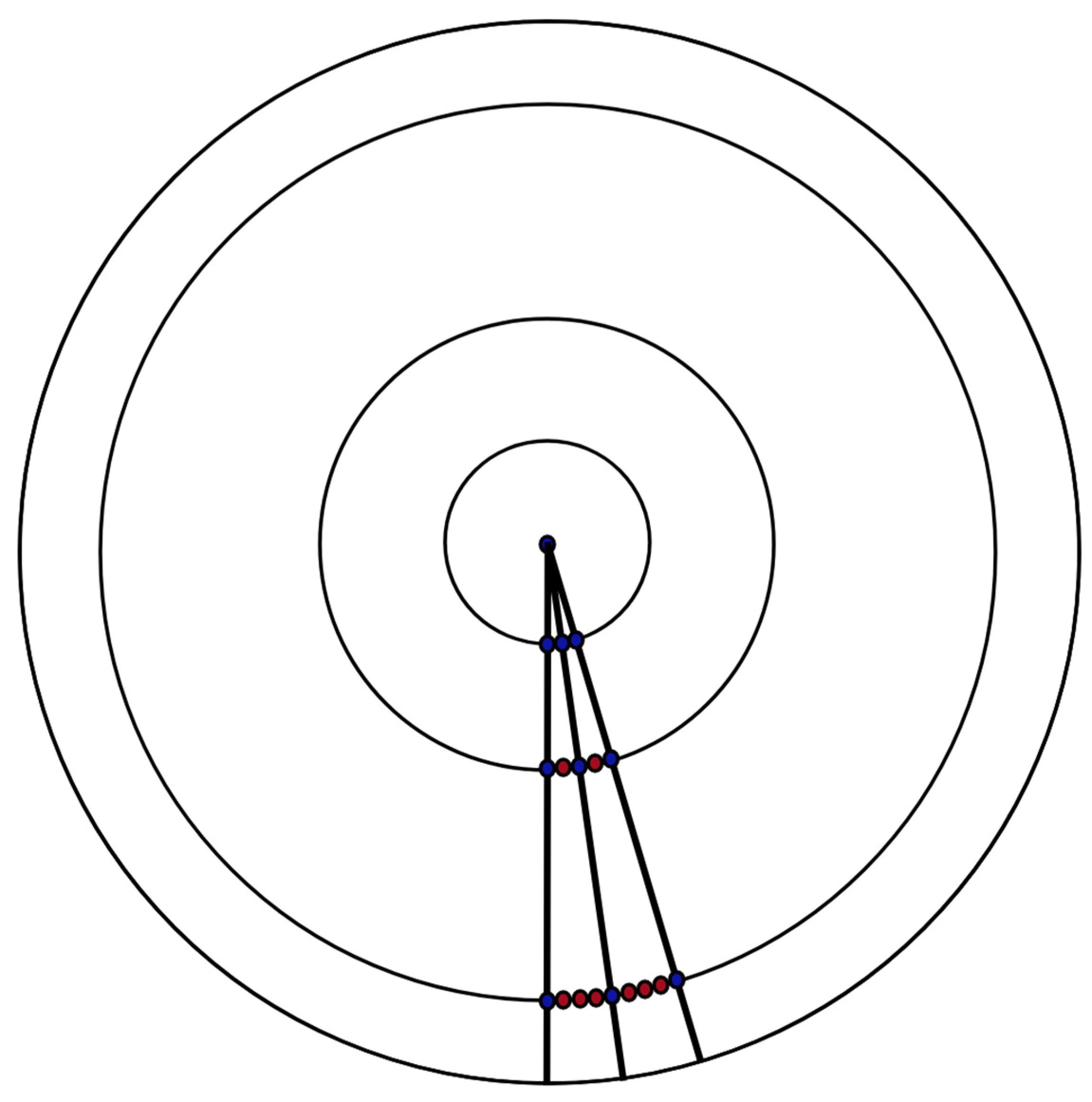
Figure 4.
Displacement of the centers of the chords (a) only along the circumference and (b) also along the radius.
Figure 4.
Displacement of the centers of the chords (a) only along the circumference and (b) also along the radius.
Disclaimer/Publisher’s Note: The statements, opinions and data contained in all publications are solely those of the individual author(s) and contributor(s) and not of MDPI and/or the editor(s). MDPI and/or the editor(s) disclaim responsibility for any injury to people or property resulting from any ideas, methods, instructions or products referred to in the content. |
© 2023 by the authors. Licensee MDPI, Basel, Switzerland. This article is an open access article distributed under the terms and conditions of the Creative Commons Attribution (CC BY) license (http://creativecommons.org/licenses/by/4.0/).
Copyright: This open access article is published under a Creative Commons CC BY 4.0 license, which permit the free download, distribution, and reuse, provided that the author and preprint are cited in any reuse.


