
Submitted:
27 March 2023
Posted:
28 March 2023
You are already at the latest version
Abstract
This article develops applications of the generalized method of lines to numerical solutions of the time-independent, incompressible Navier-Stokes system in fluid mechanics. We recall that for such a method, the domain of the partial differential equation in question is discretized in lines (or more generally in curves), and the concerning solutions are written on these lines as functions of the boundary conditions and the domain boundary shape.
Keywords:
Generalized method of lines
; Navier-Stokes system
; equivalent elliptic system
MSC: 65N40; 35Q30
1. Introduction
In this article, we develop approximate solutions for the time independent incompressible Navier-Stokes system, through the generalized method of lines. We recall again, for such a method, the domain of the partial differential equation in question is discretized in lines and the concerning solution is written on these lines as functions of the boundary conditions and boundary shape. We emphasize the first article part concerns the application and extension of an approximate proximal approach published in [3]. We develop an analogous algorithm as those presented in [3] but now for a Navier-Stokes system, which is more complex than the systems previously addressed. In this first step we present an algorithm and respective software in MAT-LAB.
Furthermore, we have developed and presented related softwares in MATHEMATICA for a simpler type of domain but also concerning the mentioned proximal approach. Finally, in the last section, we present a software and related line expressions through the original conception of the generalized method of lines, so that in such related numerical examples, the main results are established through applications of the Banach fixed point theorem.
Remark 1.
We also highlight the next two paragraphs in this article ( a relatively small part) overlaps with the Chapter 28, starting page 526, in the book by F.S. Botelho, [2], published in 2020, by CRC Taylor and Francis. However, we emphasize the present article includes substantial new parts, including a concerning software not included in the previous version of 2020. Another novelty in the present version is the establishment of appropriate boundary conditions for an elliptic system equivalent to original Navier-Stokes one. Such new boundary conditions and concerning results are indicated in Section 2.
At this point we describe the system in question.
Consider an open, bounded and connected set with a regular (Lipschitzian) internal boundary denoted , and a regular external one denoted by . For a two-dimensional motion of a fluid on , we denote by the velocity field in the direction x of the Cartesian system , by , the velocity field in the direction y and by , the pressure one. Moreover, denotes the fluid density, is the viscosity coefficient and g denotes the gravity field. Under such notation and statements, the time-independent incompressible Navier-Stokes system of partial differential equations stands for,
At first we look for solutions . We emphasize details about such Sobolev spaces may be found in [1].
About the references, we emphasize that related existence, numerical and theoretical results for similar systems may be found in [6,7,8,9] and [11], respectively. In particular [11] addresses extensively both theoretical and numerical methods and an interesting interplay between them. Moreover, related finite difference schemes are addressed in [10].
2. Details about an equivalent elliptic system
Defining now and consider again the Navier-Stokes system in the following format
As previously mentioned, at first we look for solutions .
We are going to obtain an equivalent Elliptic system with appropriate boundary conditions.
Our main result is summarized by the following theorem.
Theorem 1.
Let be an open, bounded, connected set with a regular (Lipschitzian) boundary.
Assume are such that
Suppose also the unique solution of equation in w
with the boundary conditions
is
Under such hypotheses, solve the following Navier-Stokes system
Proof.
In (5), taking the derivative in x of the first equation and adding with the derivative in y of the second equation, we obtain
From the hypotheses, are such that
From this and (9), we get
Denoting , from this last equation we obtain
From the hypothesis, the unique solution of this last equation with the boundary conditions is .
The proof is complete. □
Remark 2.
The process of obtaining such a system with a Laplace operator in P in the third equation is a standard and well known one.
The novelty here is the identification of the corrected related boundary conditions obtained through an appropriate solution of equation (10).
3. An approximate proximal approach
In this section we develop an approximate proximal numerical procedure for the model in question.
Such results are extensions of previous ones published in F.S. Botelho, [3] now for the Navier-Stokes system context.
More specifically, neglecting the gravity field, we solve the system of equations
We present a software similar to those presented in [3], with , and with
with the boundary conditions
After linearizing such a system about and introducing the proximal formulation, for an appropriate non-negative real constant K,we get
At this point denoting we define
and
Therefore, we may write
where
In particular for , we obtain
so that
where
Similarly, for we get
so that
where
Reasoning inductively, having
we obtain
where
Observe now that we have so that
This last equation is a second order ODE in which must be solved with the boundary conditions
Summarizing we have obtained
Similarly, we may obtain and
Having we may obtain with in equation (19) (neglecting )
Similarly, we may obtain and
Having we may obtain with in equation (19) (neglecting )
Similarly, we may obtain and
And so on up to obtaining and .
The next step is to replace by and repeat the process until an appropriate convergence criterion is satisfied.
Here we present a concerning software in MATLAB based in this last algorithm (with small changes and differences where we have set and ).
******************************
;
;
*********************************
4. A software in MATHEMATICA related to the previous algorithm
In this section we develop the solution for the Navier-Stokes system through the generalized method of lines, similarly as the results presented in [3], but now in a Navier-Stokes system context.
We present a software in MATHEMATICA for lines for the case in which
We consider it in polar coordinates, with , and with
and
The boundary conditions are
From now and on, x stands for .
We remark some changes have been made, concerning the original conception, in order to make it suitable through the software MATHEMATICA for such a Navier-Stokes system.
We highlight, as is larger, the related approximation is of a better quality. However if is too much large, the converging process gets slower.
Here the concerning software.
************************************************
-
(here we have fixed the number of iterations)
Here we present the related line expressions obtained for the lines , and n=9 of a total of lines.
5. The software and numerical results for a more specific example
In this section we present numerical results for the same Navier-Stokes system and domain as in the previous one, but now with different boundary conditions.
In this example, we set and the boundary conditions are
Here the concerning software:
************************************************
-
(here we have fixed the number of iterations)
-
Here the corresponding line expressions for lines
Here we present the related plots for the Lines , , and of a total of lines.
For each line we set nodes on the interval , so that the units in x are , where again x stands for
6. Numerical results through the original conception of the generalized method of lines for the Navier-Stokes system
In this section we develop the solution for the Navier-Stokes system through the generalized method of lines, as originally introduced in [4], with further developments in [5].
We present a software in MATHEMATICA for lines for the case in which
Such a software refers to an algorithm presented in Chapter 27, in [2], in polar coordinates, with , and with
and
The boundary conditions are
We remark some changes have been made, concerning the original conception, in order to make it suitable through the software MATHEMATICA for such a Navier-Stokes system.
We highlight the nature of this approximation is qualitative.
Here the concerning software in MATHEMATICA.
****************************************
- ;
-
(in this example, we have fixed a relatively small number of iterations )
***************************************************
Here the line expressions for the field of velocity , where again we emphasize lines and :
7. Conclusion
In this article, we develop solutions for examples concerning the two-dimensional, time-independent and incompressible Navier-Stokes system through the generalized method of lines. We also obtain the appropriate boundary conditions for an equivalent elliptic system. Finally, the extension of such results to , compressible and time dependent cases is planned for a future work.
References
- R.A. Adams and J.F. Fournier, Sobolev Spaces, 2nd edn. (Elsevier, New York, 2003).
- F.S. Botelho, Functional Analysis, Calculus of Variations and Numerical Methods in Physics and Engineering, CRC Taylor and Francis, Florida, 2020.
- F.S. Botelho, An Approximate Proximal Numerical Procedure Concerning the Generalized Method of Lines Mathematics 2022, 10(16), 2950. [CrossRef]
- F. Botelho, Topics on Functional Analysis, Calculus of Variations and Duality, Academic Publications, Sofia, (2011).
- F. Botelho, Existence of solution for the Ginzburg-Landau system, a related optimal control problem and its computation by the generalized method of lines, Applied Mathematics and Computation, 218, 11976-11989, (2012). [CrossRef]
- P. Constantin and C. Foias, Navier-Stokes Equation, University of Chicago Press, Chicago, 1989.
- Makram Hamouda, Daozhi Han, Chang-Yeol Jung and Roger Temam, Boundary layers for the 3D primitive equations in a cube: the zero-mode, Journal of Applied Analysis and Computation, 8, No. 3, 2018, 873-889. [CrossRef]
- Andrea Giorgini, Alain Miranville and Roger Temam, Uniqueness and regularity for the Navier-Stokes-Cahn-Hilliard system, SIAM J. of Mathematical Analysis (SIMA), 51, 3, 2019, 2535-2574. [CrossRef]
- Ciprian Foias, Ricard M.S. Rosa and Roger M. Temam, Properties of stationary statistical solutions of the three-dimensional Navier-Stokes equations, J. of Dynamics and Differential Equations, Special issue in memory of George Sell, 31, 3, 2019, 1689-1741. [CrossRef]
- J.C. Strikwerda, Finite Difference Schemes and Partial Differential Equations, SIAM, second edition (Philadelphia, 2004).
- R. Temam, Navier-Stokes Equations, AMS Chelsea, reprint (2001).
Figure 1.
Solution for the case .
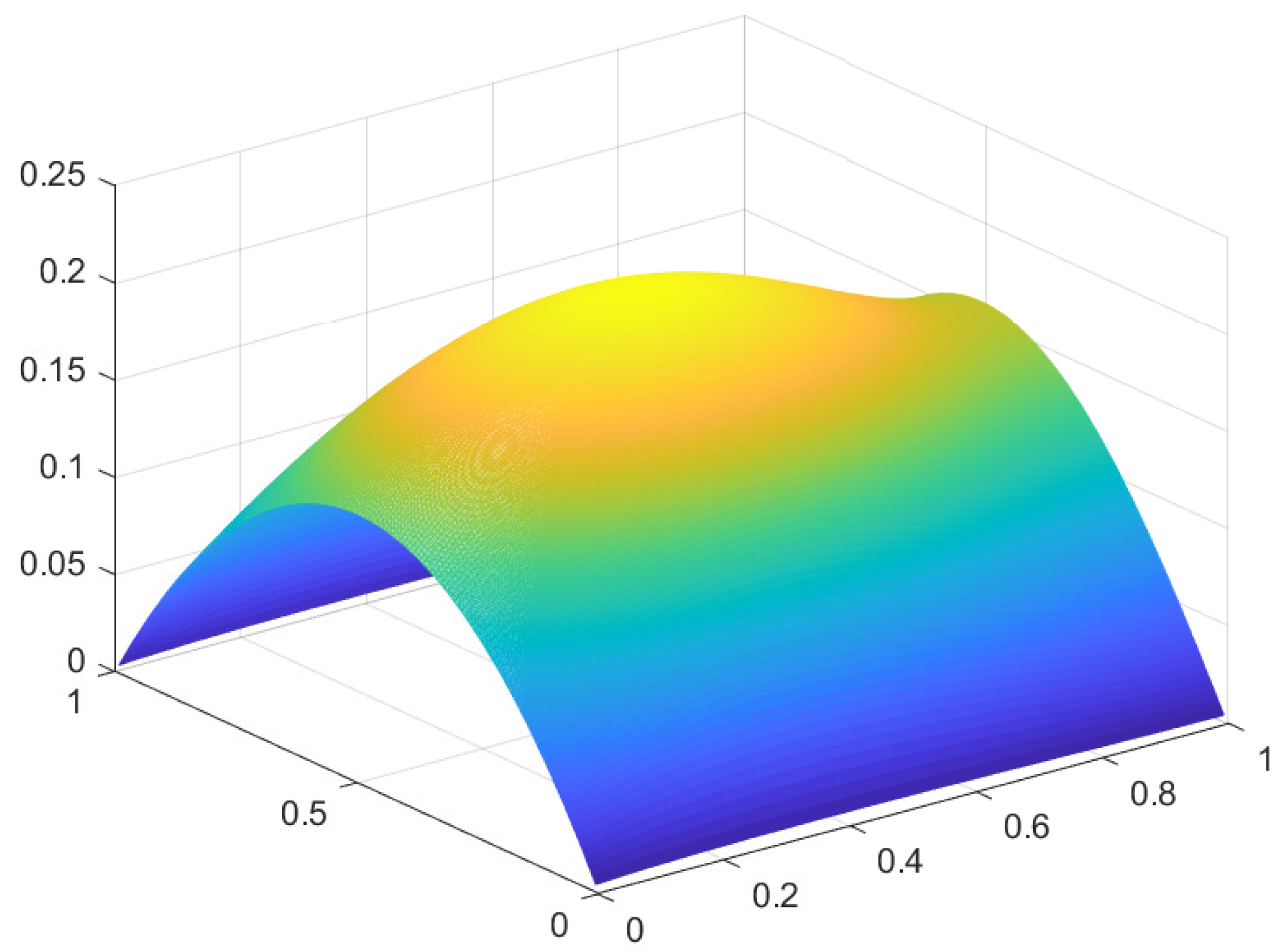
Figure 2.
Solution for the case .
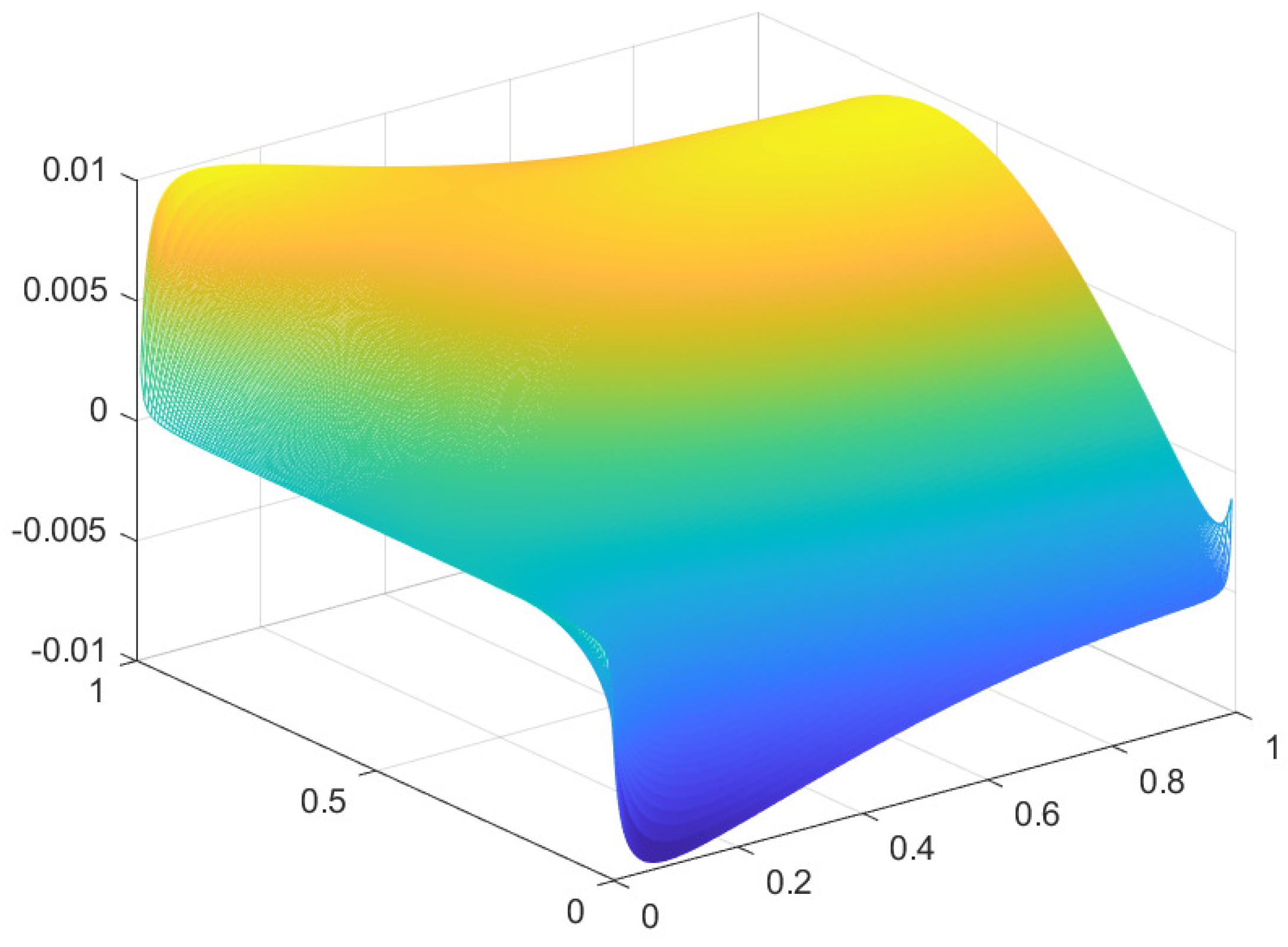
Figure 3.
Solution for the case .
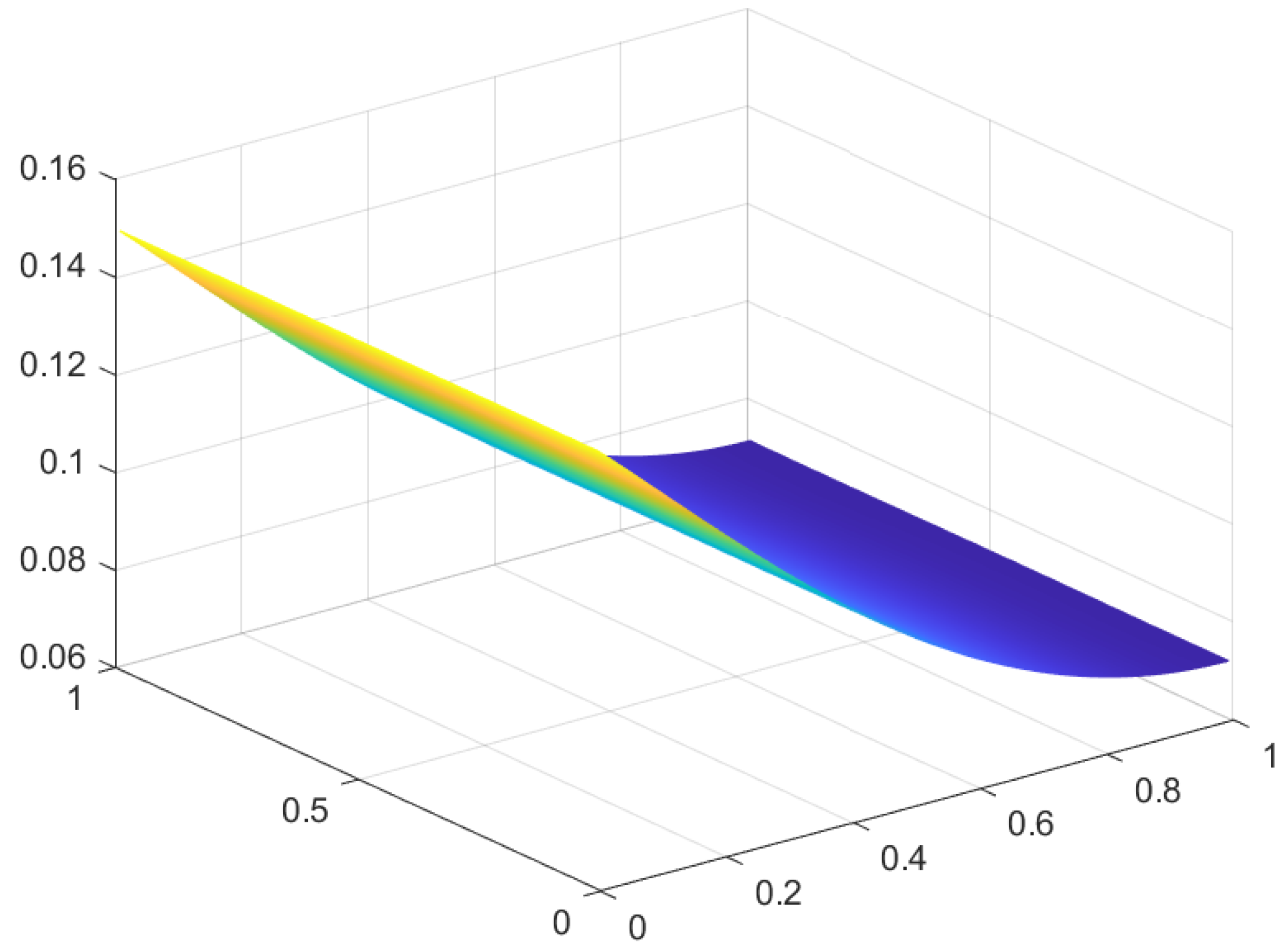
Figure 4.
Solution for the line , for the case .
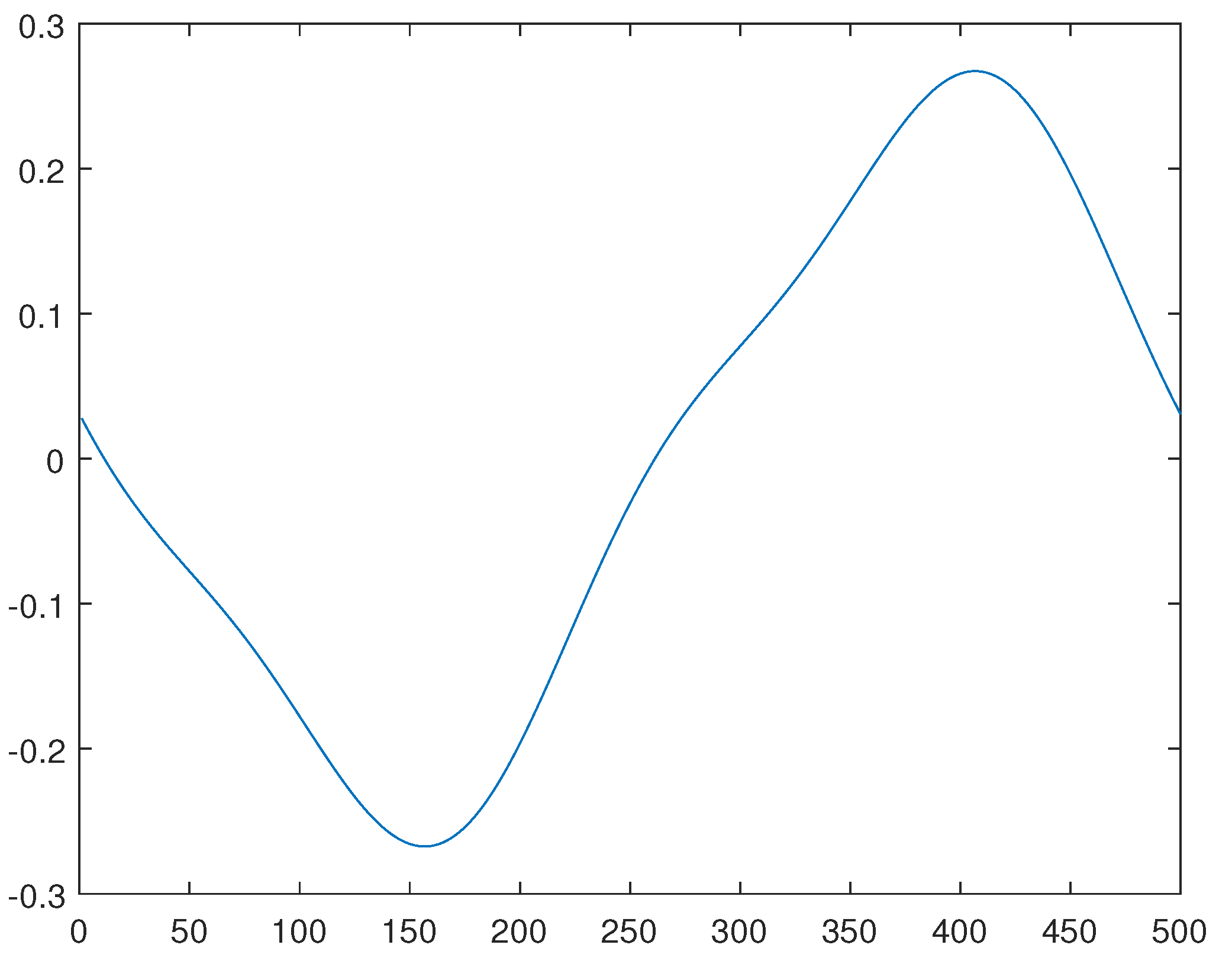
Figure 5.
Solution for the line , for the case .
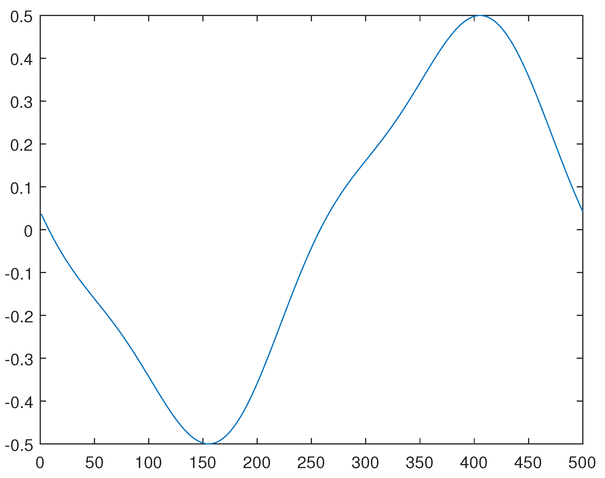
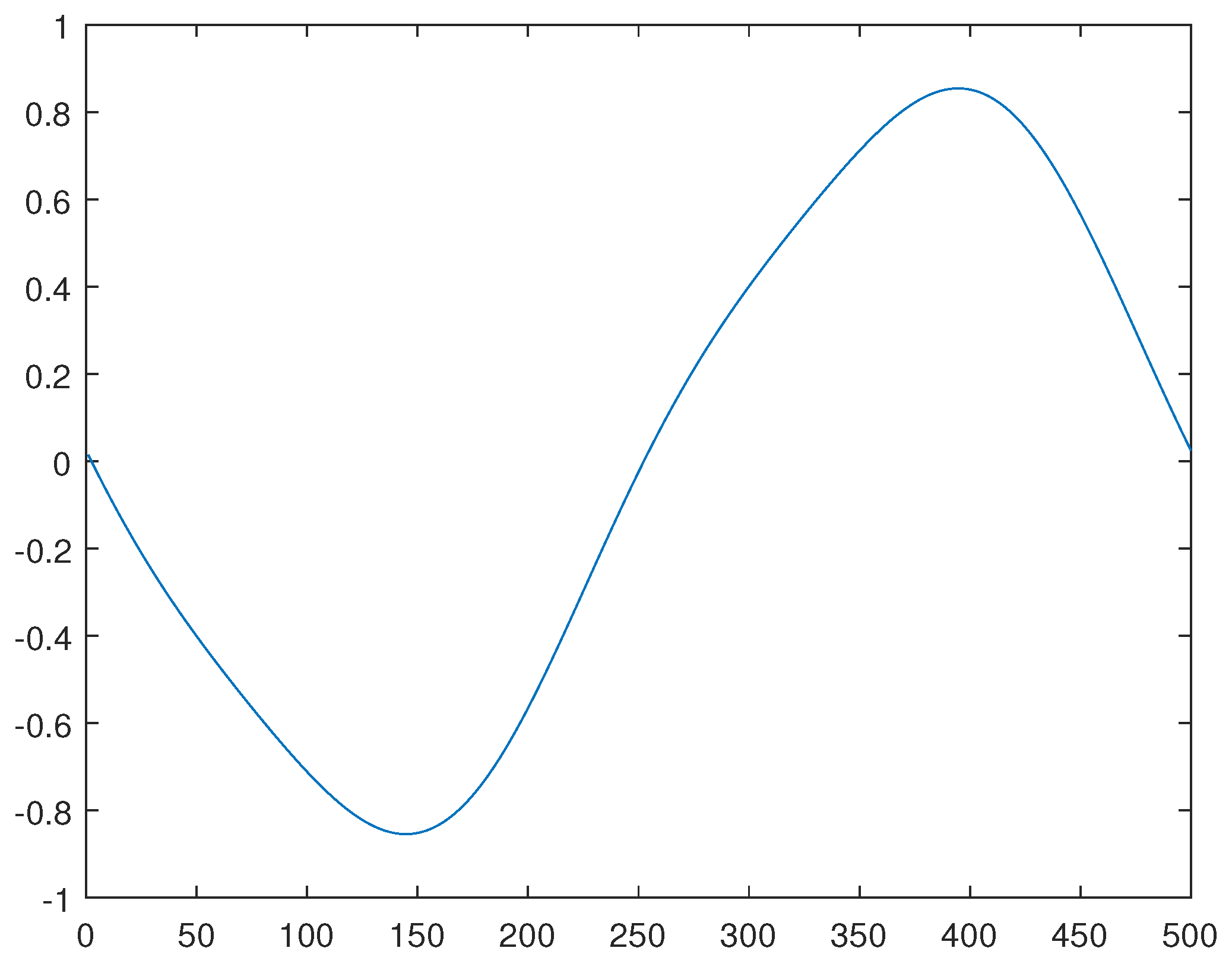
Figure 6.
Solution for the line , for the case .
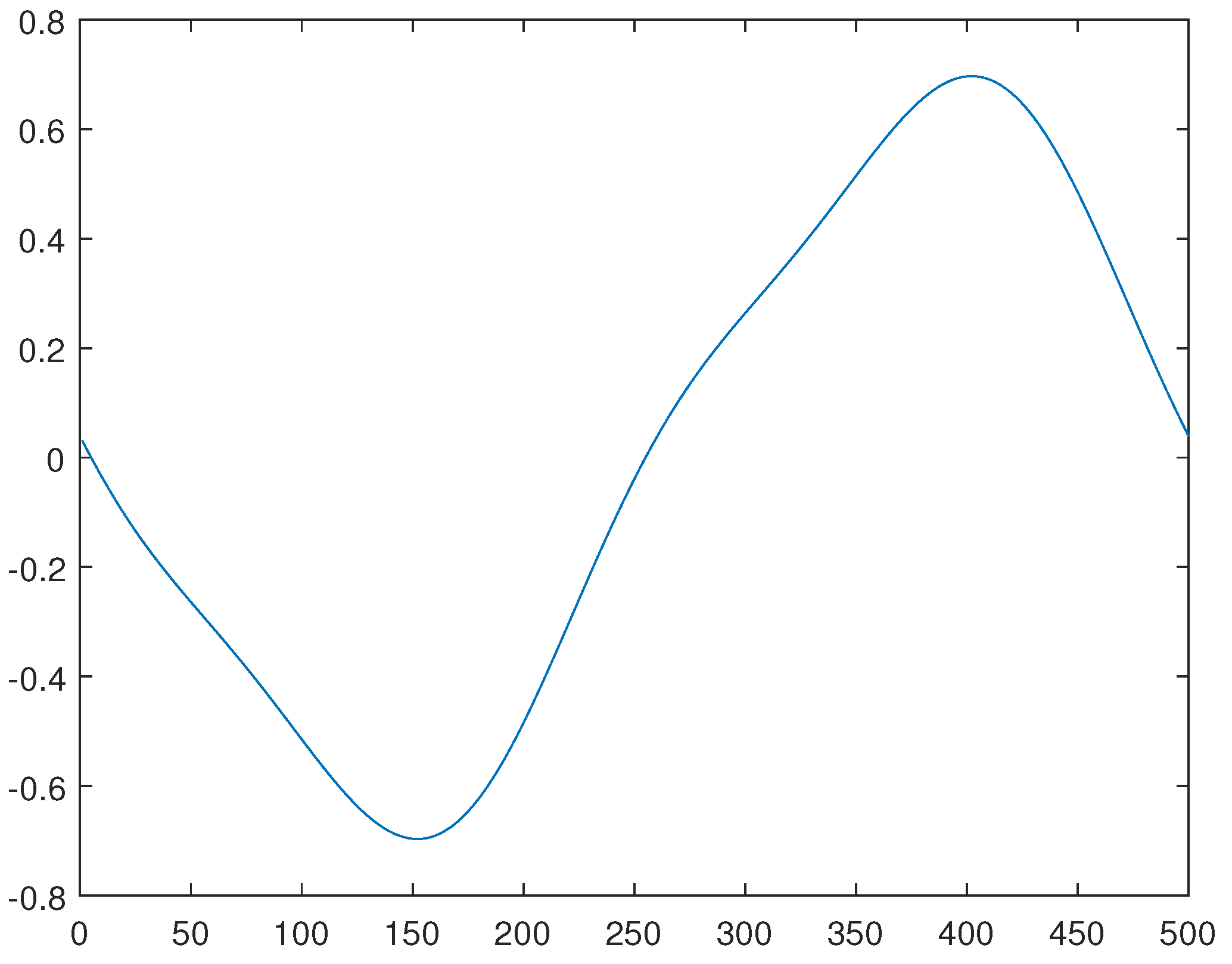
Figure 7.
Solution for the line , for the case .
Disclaimer/Publisher’s Note: The statements, opinions and data contained in all publications are solely those of the individual author(s) and contributor(s) and not of MDPI and/or the editor(s). MDPI and/or the editor(s) disclaim responsibility for any injury to people or property resulting from any ideas, methods, instructions or products referred to in the content. |
© 2023 by the authors. Licensee MDPI, Basel, Switzerland. This article is an open access article distributed under the terms and conditions of the Creative Commons Attribution (CC BY) license (http://creativecommons.org/licenses/by/4.0/).
Copyright: This open access article is published under a Creative Commons CC BY 4.0 license, which permit the free download, distribution, and reuse, provided that the author and preprint are cited in any reuse.


