Quantifying the Effects of Different Containment Policies on Urban NO2 Decline: Evidence From Remote Sensing Integrated With Ground-Station Data

Cities exposed their vulnerabilities during COVID-19 pandemic. Unprecedented policies restricted human activities but left an unique opportunity to quantify anthropogenic effects on urban air pollution. This study aimed to address the key questions of urban development behind the restrictions with the goal of supporting sustainable transition. Data from ground stations and Sentinel-5P satellite were used to assess the temporal and spatial anomalies of NO2. Beijing China was selected for a case study because this mega city maintained a “dynamic zero-COVID” policy with adjusted restrictions, allowing us better to track the effects. The time-series decomposition and prediction regression model were employed to estimate the normal NO2 levels in 2020. The anomalies between the observations and predictions as the deviation were identified due to the policy interventions and quantified different effects using spatial stratified heterogeneity statistics. The top three restrictions showing dominant effects were workplace closures, restricted public transport usage, and school closures, accounting for 54.8%, 52.3%, and 46.4% of NO2 anomalies, respectively; and they are directly linked to the mismatch of employment and housing (deter-mining the commuting patterns), educational inequality and the long-term unsolved road con-gestion. Promoting the transformation of urban spatial structure will effectively alleviate air pollution.

Keywords:

Subject: Environmental and Earth Sciences - Environmental Science

1. Introduction

Nitrogen dioxide (NO₂) is a common air pollutant that can harm the environment and human health. The mainly anthropogenic NO₂ emissions was reported from the transport sector, industry, power, heating and residential sector [1,2]. Exposure to NO₂ has been linked to many respiratory diseases [3]. Chronic exposure to NO₂ pollution led to a higher mortality rate during the COVID-19 pandemic [4] and these pollutants affected virus transmission [5]. Triggered by the pandemic, air pollution and traffic were identified as two of the top six environmental challenges facing cities [6]. Unprecedented strong policy measures, as nonpharmaceutical interventions, were taken worldwide, especially in urban areas, restricting human activities and industrial production. The strict restrictions directly affected the emissions of various air polluting gases, and in turn, such changes in global and regional emissions may reflect the effects of different policies. In this context, a consensus has been proposed that this "pause button" created an unique window to assess anthropogenic effects on atmospheric composition and its relationship to human activities compared to “business as usual”. More importantly, it calls for extensive actions that can make full use of this “anomaly” opportunity to boost our cities shift to sustainability [6], as sustainable development depends increasingly on the successful management of urban growth. NO₂ has been considered a good indicator of changes in local pollutant sources, as it has a shorter lifetime (within 1 day) compared with other air pollutants [7]. Therefore, in this study, the sensitivity of NO₂ to policy responses during the COVID-19 pandemic can be captured or tracked by restriction measure changes on daily-scale. It provides an observational metric for examining the effects of diverse policy regulations on air pollution, reducing the complexity due to the hysteresis of some policy effects. It is important for understanding which policies (linked to different human activities) are effective in reducing emissions.

At the early stage of the epidemic, the observation-based concentrations of NO₂ pollutants were consistently reported to be below the levels of previous years, as a result of the sudden lockdowns and suspended human activities. Data from both satellite observations and ground-based monitoring stations found that global NO₂ concentrations were lower in 2020 than in 2019, especially in urban areas [7,8]. In Wuhan, China, the first reported outbreak city, the NO₂ in 2020 during lockdown was 42% lower than the average level of the previous three years [9]. The reduction in transport sector emissions is reported as the main cause for global NO₂ anomalies [8]. London experienced a 50% decrease in NO₂ during lockdown, with the highest NO₂ emission reductions observed during morning rush hours due to the radical changes in routine life and commuting time [10]. Observations from other mega-cities, such as New York [11], Tokyo [12], Moscow [7] and Toronto [13], also showed a decrease in NO₂ concentrations during lockdowns. Nevertheless, some subsequent studies noted the possibility of exaggerating the positive effects of COVID-19 policies and pointed out that the improvement in air quality was not due to COVID-19 interventions but seasonal factors, as the lockdown period coincided with the onset of the rainy season in tropical regions, such as in Nigeria [14] and Indonesia [15]. This observation arises from the fact that most studies reported improvements in air quality based on comparisons between lockdowns and pre-lockdown periods or by taking the previous 3- to 5-year average level as the baseline. Some review papers investigated the nexus between the pandemic and the environment, showing that meteorological conditions affected NO₂ concentrations [15,16].

With continuous discussions on this popular topic and the accumulation of available multisource datasets, recent studies have begun to use the sensitivity changes of NO₂ to infer, correlate and retrieve various phenomena, consequences or environmental indicators related to it. In this context, ground-based instruments, alone or combined with satellite observations (e.g., from Ozone Monitoring Instrument (OMI) on-board Aqua satellite, Tropospheric Monitoring Instrument (TROPOMI) on-board Sentinel-5P), provide fundamental information about anthropogenic impacts. The stringency of policy indicators has been used for investigating certain impacts on the environment. Long-term temporal comparisons of tropospheric NO₂ vertical columns during the lockdown with the counterfactual baseline concentrations have been investigated with different extensions and specific perspectives. For example, Misra et al. [17] retrieved the NO₂ concentration changes due to lockdown from OMI and TROPOMI and linked the changes to power plants over urban areas in northern India while considering the seasonal components of NO₂ and long-term trends over the same period in 2015-2019. Xing et al. [5] used machine learning with multisource data to prove that reduced economic activity, inferred from NO₂ reductions (restrictions-induced), drove the slowdown in the number of COVID-19 infections in most regions [5]. Highlighting that pollution has no borders, Li et al. [18] clustered global continent grid cells, which were based on historical NO₂ pollution levels from OMI satellites for which seasonal trends had been removed, by subtracting 10-year daily mean values to investigate the impact of policy stringencies on different clusters (regions). There are significant differences between regions due to differences in measures taken, the duration of lockdowns, and the intensity of measures implemented by the government, which allows much potential for in-depth explorations.

Most of the existing studies documented the short-term positive effects of containment policy measures on declining air pollution; however, the long-term effects have not been fully considered, especially for other confounding factors, such as seasonality, climate conditions, air quality improvement trends and the local context. It may exaggerate the effects of covid-19 restrictions. Furthermore, few evidence-based methodologies could identify the effective policy which has direct impact on the NO₂ anomaly and linked to specified human activities. In other words, very limited efforts have been made to differentiate and quantify the effects of different policies. This challenge may be a barrier for policy-makers or create indecision when effective actions are considered.

To fill the research gaps discussed above, in this study, we proposed that observations combined with predictions. We employed historical ground-station data combined with Sentinel-5P data to illustrate the sensitivities of NO₂ concentrations to different policy measures of COVID-19. Particularly, we estimated the portion of NO₂ anomalies caused by COVID-19 restriction policies by removing the confounding factors. The spatial and temporal variations of NO₂ were visualized for interpretations based on remote sensing. Ultimately, this study applied spatial stratified heterogeneity statistics in time-series analysis; and by linking the daily-scale variations of containment measures to NO₂ anomalies, we quantified and ranked the contributions of different policies. Such analysis is expected to generate a more reliable and accurate evaluation of the effects of different restriction policies on human activities that reflect on NO₂ anomalies. It is essential to evaluate how policies can further guide human activities as cities transition to environmental sustainability during their post-epidemic recoveries. Furthermore, this evaluation may help shed light on some uncertainties regarding future global and regional climate responses to polluting gas emissions.

2. Study Area and Data

2.1. Study Area

In this study, Beijing was selected as the study area, as shown in Figure 1. There are three main reasons. Firstly, Beijing is the capital of China, with a large population and highly concentrated economic activities. China was the first country to implement lockdown measures and adopt the “dynamic zero COVID-19” policy (i.e., adjusting policies dynamically, according to the infection situation until the time of writing). This context allows the diversity changes in NO₂ before, during and after policy interferences to be tracked. The difference between the expected NO₂ level under “business as usual” conditions and the actual levels during the COVID-19 pandemic can be described as an “anomaly”. Secondly, Beijing has been facing severe air pollution problems compared to other cities in China: NO₂ pollutants were reported to have exceeded the standard by 40% in 2013 [19]. The city’s air quality has been improved due to specific control policies in recent years, including promoting new energy vehicles, shutting down high-emission waste factories and imposing technological transformation [20,21], etc. These types of “structural” control measures may have long-term accumulation effects on NO₂; and the geographical location of this city allows it having four distinct seasons. Thirdly, there are some investigations on this city that can be compared for validation. More specifically, NO₂ concentrations derived from TROPOMI in Beijing decreased by 45% in March 2020 [9], while ground-based NO₂ concentrations in Beijing decreased by 41.8% compared with the previous 3-year average level, and by 33.7% compared to 2019 [22]; one recent study from global perspective, showed that the COVID-19 outbreak explained reductions in NO₂, from OMI and TROPOMI, by only 6% averagely in China when considering meteorology effects[7]. Another globally study based on OMI showed that NO₂ level between January and February was seen a drastic reduction while it further observed to rise in the March and April 2020 [18]. As spatial heterogeneity of NO₂ anomalies have been confirmed, the differences between observations recall that research findings may vary due to different spatial scales regarding the Modifiable Areal Unit Problem (MAUP) [23]. Besides, this “dynamic zero COVID-19” policy, as an experimental case here, may also provide the comparative references to other countries and regions in terms of implementing different policies.

2.2. Data

2.2.1. Ground-station data

This study collected in situ station data from Air Quality Open Data Platform (https://aqicn.org/data-platform/covid19/), supported by the World Air Quality Index Project. We obtained NO₂ concentration data for the five years before the COVID-19 pandemic (2015-2019) and one year during COVID-19 (2020). The original time series datasets from the Beijing Environmental Protection Monitoring Center (http://zx.bjmemc.com.cn/) were used for the long-term time-series modelling (see Section 3), and for the 5-year average baseline calculation. There are 35 ground-stations located in the city currently where the 12 stations were densely located in the main six urban districts, and others were distributed in the suburban and rural areas. Each ground station can provide NO₂ concentration measured in micrograms in each cubic meter of air (µg/m³). It can monitor the timely NO₂ changes at the specific location (hourly or even higher temporal resolution). Figure 1 showed the distributions of these ground stations that they cannot cover the whole regions, while they may reflect the most sensitive areas with anomalies. In this study, the daily average of NO₂ concentration datasets from all city ground stations were used.

2.2.2. Remote sensing observations

Satellites can observe the spatial variations in NO₂ that surface observations cannot. It can fill the gaps between ground monitors, including unmonitored regions where no ground stations are located. In this study, we used Sentinel-5P satellite data, which is dedicated to monitoring trace gases, to acquire NO₂ data for 2019-2020. Existing studies have shown that TROPOMI measurements are well correlated with ground-based NO₂ data from situ stations [25,26]. As the NO₂ data was released from TROPOMI from July 2018 and cannot be used yet for long-term analysis, we combined it with in situ station data to better understand the long-term trends and seasonal effects.

The TROPOMI on Sentinel-5P has improved observation capabilities that can provide a finer spatial resolution (1 km) imagery of NO₂ monitoring. It can provide daily observations with a “column” concentration, that is, tropospheric NO₂ column number density (mol/m²), the indicator used in this study. It cannot avoid the cloud cover effects; therefore, we filtered out pixels that are fully or partially covered by clouds, using 0.2 as a cutoff for the radiative cloud fraction. The processing of remote sensing data was conducted on Google Earth Engine (GEE, https://earthengine.google.com/) for geospatial analysis with cloud computing. The released NO₂ datasets on GEE is the Level-2 (L2) data products which has been calibrated and validated (more data preprocessing information can be found in the user handbook: https://sentinel.esa.int/documents/247904/2474726/Sentinel-5P-Level-2-Product-User-Manual-Nitrogen-Dioxide.pdf).

2.2.3. Climate data

Apart from anthropogenic effects, the changes of NO₂ concentrations were affected by meteorological effects [27] and seasonal variability. Therefore, this study collected the climate datasets of ERA5-Land during 2015 to 2020 from the Copernicus Climate Data Store https://cds.climate.copernicus.eu/. ERA5-Land is a reanalysis dataset providing a consistent view of the evolution of land variables over several decades at an enhanced resolution. Some meteorological factors were collected, including temperature of air at 2 m above the surface of land, total precipitation, Eastward and Northward component of the wind at a height of ten meters above the surface of the Earth, and pressure (force per unit area) of the atmosphere on the land surface. This data was used to examine the relationship between NO₂ concentration and meteorological conditions.

2.2.4. Daily policy tracking indicators

To examine the relationship between COVID-19 lockdown policies and ground-level NO₂ concentrations, we used Oxford University's COVID-19 Government Response Tracker data (OxCGRT, https://www.bsg.ox.ac.uk/research/research-projects/coronavirus-government-response-tracker#data). This dataset categorizes and grades policy measures according to each country's intensity and timing of implementation. OxCGRT provides digital indicators based on containment and closure policies, including those directly linked to different social activities (e.g., school and workplace closures, restricted public transport stay-at-home orders, gathering restrictions and border measures). We selected policy data from Beijing, China [28] to precisely track which policies were implemented and at what level each day. The focus of the research is to analyze the relationships between the policy implementation, dynamic change characteristics and NO₂ emissions using time series analysis and modeling. The containment policies (C1-C8) selected for analysis (more details can be found in Figure A1).

3. Methodology

The methodological workflow proposed in this study is shown in Figure 2. The time-series analysis was conducted based on historical ground station datasets from 2015 to 2020 to detect the compounding factors that may affect NO₂ changes. By further combining with climate data, a time-series prediction regression model was developed to estimate the expected NO₂ level of 2020 (no COVID-19 restrictions). The NO₂ anomaly between observations and predictions were used to build Stratified Heterogeneity statistical model (Geodetector) for evaluating the effects of different containment policies. From spatial aspects, Sentinel-5P observational data for 2019 and 2020 were used to capture the distributions of spatial differences of NO₂.

3.1. Time series modelling

This study first employed time series models to analyze the long-term trends and seasonal effects on NO₂ emissions, so as to further determine the extent to which the changes are due to the COVID-19 policy measures. Specifically, using ground-based observation data for the five years before the pandemic, a time series X11 decomposition model was used to detect the change trend and periodic impact characteristics of the long-term series, and a multiple linear regression model was used to build a time series prediction model. Together, this allows the estimation of the NO₂ emission curve under “business as usual” conditions, that is, the expected line for 2020 without the intervention of the COVID-19 restriction policies. The time-series analysis and modelling were completed using R.

3.1.1. Decomposition model

A time series decomposition model was used to detect and decompose a series into a set of unobservable (latent) components that can be associated with different types of temporal variations, for example, (1) a long-term trend; (2) cyclical movements superimposed upon the long-term trend; (3) seasonal variations that represent the composite effect of climatic and institutional events which regularly repeat each year; and (4) the irregular component (changes in NO₂ levels which are unexpected). Since seasonality ultimately results mainly from geographical differences and a whole suite of climatic factors, its impacts on NO₂ cannot be modified in a short period of time. Therefore, it is of interest for policy making and evaluation purposes to remove seasonal variations from the original series. The long-term trends affected by local AQ policy apply here as well.

The X11 time series decomposition model was used to determine the trend and seasonality of the time series [29], with the decomposition formula:

y_{t} = T_{t} \times S_{t} \times R_{t}

(1)

where

T_{t}

represents the smoothed trend term,

S_{t}

represents the seasonal term, and

R_{t}

represents the residual term (refers to irregular component).

Using the X11 time decomposition prediction model, the NO₂ observation curves can be decomposed into the seasonality curve (natural cycle), long-term trend, and irregular components.

3.1.2. Prediction regression model

We employed a multiple linear regression to build a time-series prediction regression model. Trends, seasonal dummy variables (monthly) and climate factors (temperature, precipitation, wind and surface pressure) were selected as the predictor variables; the dependent variable Y is the logarithm of NO₂ data from the ground-stations. We used daily data (i.e., 5 years * 365 days of continuous observation data) and monthly data (i.e., 5 years * 12 months of data per year) for the time series regression analysis respectively and evaluated each model's performance. We modeled this time-series data using a multiple regression model with a linear trend and monthly dummy variables, using the following formula:

y_{t} = β_{0} + β_{1} x_{1, t} + β_{2} x_{2, t} + \dots + β_{k} x_{k, t} + ε_{t}

(2)

where

y_{t}

is the NO₂ variable to be forecast and

x_{i}

is the predictor variables; here, they refer to three parts, that is the linear trend, seasonal dummy variables (0~11 for 12 months), and climate variables. The coefficient

β_{i}

measure the marginal effects of the predictor variables.

ε_{t}

represents a deviation from the underlying straight line (linear regression) model, thus it captures anything that may affect

y_{t}

other than

x_{t}

. Therefore, the conceptual regression formula can also be expressed as:

\log ({N O}_{2}) = t r e n d + s e a s o n + c l i m a t e + ε_{t}

(3)

3.2. Geodetector model

Geodetector is a statistical method to detect Stratified Heterogeneity (SH) and reveal the driving forces behind it, without the assumption of linearity of the association. It was originally developed in the context of medical geography and can be applied to analyze categorical data [30,31]. The terms “SH” can refer to either spatial (spatial stratified heterogeneity, SSH) or non-spatial data such as time-series. In this study, the model was used to construct a time series analysis in order to evaluate the impact of different policy intensities and time on NO₂ emission anomalies during COVID-19. The time series analysis we performed on this data was with a daily granularity. The degree of correspondence between layers X and Y is measured by the power of determinant (q) for a factor X, and the q-statistic is defined as:

q_{x} = 1 - \frac{\sum_{h = 1}^{L} N_{h} σ_{h}^{2}}{N σ^{2}} = 1 - \frac{S S W}{S S T}

(4)

S S T = \sum_{i}^{N} {(Y_{i} - \bar{Y})}^{2} = N σ^{2}

(5)

S S W = \sum_{h = 1}^{L} \sum_{i}^{N_{h}} {(Y_{h i} - {\bar{Y}}_{h})}^{2} = \sum_{h = 1}^{L} N_{h} σ_{h}^{2}

(6)

where the time-series data is composed of N units and is stratified into h = 1, 2, …, L stratum; here it refers to the category of policy measures, so L=8; stratum h is composed of

N_{h}

units, in this case 365 (days for one year of 2020);

σ^{2}

is the population variance;

Y_{i}

and

Y_{h i}

represent the value of unit i in the population and in stratum h, respectively; and SSW and SST represent the Within Sum of Squares and the Total Sum of Squares, respectively. The value of q is within [0, 1], the larger the value of q, the stronger the explanatory power of independent variable X to Y. In other words, a q value indicates that X explains 100×q% of Y: q = 0 indicates that there is no coupling between Y and X; q = 1 indicates that Y is completely determined by X.

Here, the q statistic is used to explain “which policies have a dominant effect on NO₂ emission anomalies and what are their rankings?” The input of the Y value is the difference between the observed value of NO₂ in 2020 and the predicted value from prediction model in Section 3.1.2, which was designed to remove the seasonality and long-term trend sector, and to consider the change section due to the COVID-19 policies. X(X1~X8) refers to C1~C8 containment policy implementation and the value (category) is for each policy factor. The input data was processed in a time series format and processed in R.

4. Results

4.1. Seasonality and Trend

From the six-time series shown in Figure 3, NO₂ concentrations show a certain seasonal distribution pattern (annual periodicity), which is generally at a low level from March to September each year and then has high peaks in winter, especially in November and December. The meteorological factors show obvious seasonal characteristics, especially in the annual periodic changes.

From the X11 time series decomposition in Figure 4, the original NO₂ curves on the top consist of multiplying the three components below, that is trend, seasonal and irregular components. It can be seen from the figure that after removing the effects of seasonal and irregular components, NO₂ showed a downward trend. Besides, the decomposition shows obvious seasonal periodic features where there is a nearly robust seasonal component, with no big change between every year. Seasonality and gradual downward trends were detected, which should not be ignored in terms of analyzing the effects of policy measures on NO₂ emissions during COVID-19. The irregular component shows unexpected changes which may reflect different policies at different times during the COVID-19 pandemic. The residual item is found by subtracting the seasonal item and the trend item from the original time series data. These residual items distributed at each time node reflect disturbances due to certain events or policy measures. The implementation of the strict lockdown policy can be traced in the first half of 2020, from March to July. In addition, a number of significant air quality control measures that were implemented in September 2017 could also be traced on the timeline, for example, the closing of several coal-fired power plants and phasing out of more than 2 million high-emission vehicles. The long-term downward trend may be related to these structural emission reduction policies which have been implemented in recent years in Beijing.

4.2. Prediction versus Observation

From the time-series prediction model, we obtained the expected NO₂ value (prediction results) for the “business-as-usual” condition, as shown in Figure 5. In this case, the time-series prediction covered the seasonality and a downward trend as the above section indicates; comparing the observed NO₂ in 2020 and this prediction result gives the NO₂ anomaly due to COVID-19 policy interventions. Compared with the prediction line, the observed NO₂ in 2020 decreased on average by 6.03% for the whole year, exceeding the expected level. In particular, from March to June 2020, the observed NO₂ level was significantly lower than the predicted line, with the largest decrease of 17.04% recorded in March. This period coincided with the implementation of strict lockdown policies; as the pandemic situation improved in the second half of the year, policies were dynamically adjusted, and economic activity gradually recovered. A rebound peak appeared in October and November, showing an even higher NO₂ emission than the expected (non-COVID-19) level, though it was still below the 5-year average baseline.

Compared with the 5-year average level, NO₂ observed in 2020 was significantly lower, with an average decrease of 14.10% and the largest decrease in March (23.92%). However, it should be noted that since 2018, it has been lower than the baseline. The rebound peak would be hard to detect if only comparing with previous average data and not removing the other factors (seasonality and the downward trend). We also compared the results with the 2019 data. This showed that the expected NO₂ levels in 2020 would be expected to decrease by 2.68%, while the actual NO₂ levels in 2020 decreased by 8.60%. Table 1 presents a more detailed comparison between observed and expected values.

4.3. Interpretations from Remote Sensing

The differences in the spatial distribution of NO₂ were detected using remote sensing data. Using spatial raster calculations between 2019 and 2020, the spatial NO₂ changes show where decreases and increases have taken place (Figure 6). From February to July 2020, the urban areas maintained a consecutive and significant reduction of NO₂, especially in the economically developed northern urban areas of Beijing. Meanwhile, suburban areas with relatively low population density and less economic activities had less changes. This shows that the implementation of the policy had the greatest effect on the economically developed and populated urban areas. From August to December 2020, NO₂ in some places increased but declined in other places, which is evident from the remote sensing data but not when average aggregated data for the whole city is used. For example, the line graphs of NO₂ levels measured with ground-station data show that there was a NO₂ rebound anomaly in November 2020, which was higher than the expected results, but the remote sensing data shows spatial differences. This may indicate that some conditional economic recovery activity (coexistence with the pandemic mode) led to spatial heterogeneity of production activities. Combined with the satellite observation, it showed NO₂ concentrations in the urban center area mainly decreased, while the southern urban area showed an increasing trend from September to December. This increase may be related to flight activity following the reopening of Daxing International Airport and the recovery of industrial activity. In addition, winter heating related to burning fossil fuels may also account for the high levels in November and December 2020.

4.4. Quantifying different policy effects on NO₂ anomalies

The model results show that the dominant factors and level of influence of factors can be ranked according to their q values, namely C2 >C5>C1 >C3 >C6 >C7 >C8>C4, as Table 2 shows. Note that the “dominant” factor here means that when it has a larger q value, it will have a relatively larger impact than other factors.

Specifically, among the measures, C2 “Workplace closing” had the greatest effect, explaining 54.8% of NO₂ anomaly. This is likely to be because the C2 policy directly affected people's commuting activities. The second most influential policy was C5 “Close public transport”, which explained 52.3% of the NO₂ anomaly. This is consistent with many existing studies, which find that the transportation sector affected reductions in NO₂ during the COVID-19 pandemic [10,11]. The third dominant factor is C1 “School closing”, where school closure measures explained 46.4% of the NO₂ anomaly. It was close to the influence of C3 “Cancel public events” (44.8% explained). The fifth explanatory variable was C6 “Stay at home requirements”, which explained 42.1% of the NO₂ anomaly. The top five dominant factors are all related to people's travel activities.

The sixth explanatory variable was C7 “Restrictions on internal movement”, that is, restricting people's movements within the city. After the implementation of the green code system and the precise division of high-medium-low risk areas in Beijing, this measure mainly refers to restricting the flow of people from high-risk areas to other areas. At the same time, people in non-high-risk areas were also advised not to travel to high-risk areas unless necessary. The last two impact factors are C8 “International travel controls”, which restricted international flights and C4 “Restrictions on gatherings”, which restricted population gatherings of different sizes. These last three policy factors were once considered to be the most effective means of controlling the spread of the virus, but under the “dynamic zero-COVID” policy in China, these policy measures have had the least impact on the reduction of NO₂ emissions. It indicates that controlling the routine activities within the city had higher impacts on NO₂ changes than controlling inter-city activities.

Significant differences can be seen between the levels of implementation of the various policies, that is, when a policy is not taken (e.g., no measures=0), not enforced (e.g., recommended=1), and enforced (e.g., different intensity for 2~4). However, the conditional threshold and limit size of the specific levels of implementation need further exploration. For example, our preliminary results show that the impact of C2, level 2 (require closing (or work from home) for some sectors or categories of workers) is the most important, rather than all closing or other levels. Another example can be seen in the differences in the levels of C4 “Restrictions on gatherings”, where the effect was most pronounced when the population size was limited to less than 100 people. Further research is needed on how to design the effective policy threshold for guiding a new balance between low air pollution and people's lifestyles, as well as other policymaking objectives.

5. Validation

We evaluated the effectiveness of the model from each indicator shown in Figure 7. In the process of model selection and calculation, we processed all data as time series data. First, we selected climate data (temperature, precipitation, wind and surface pressure) as the independent variables, as has been done for regression modelling for air pollution estimates in many studies. 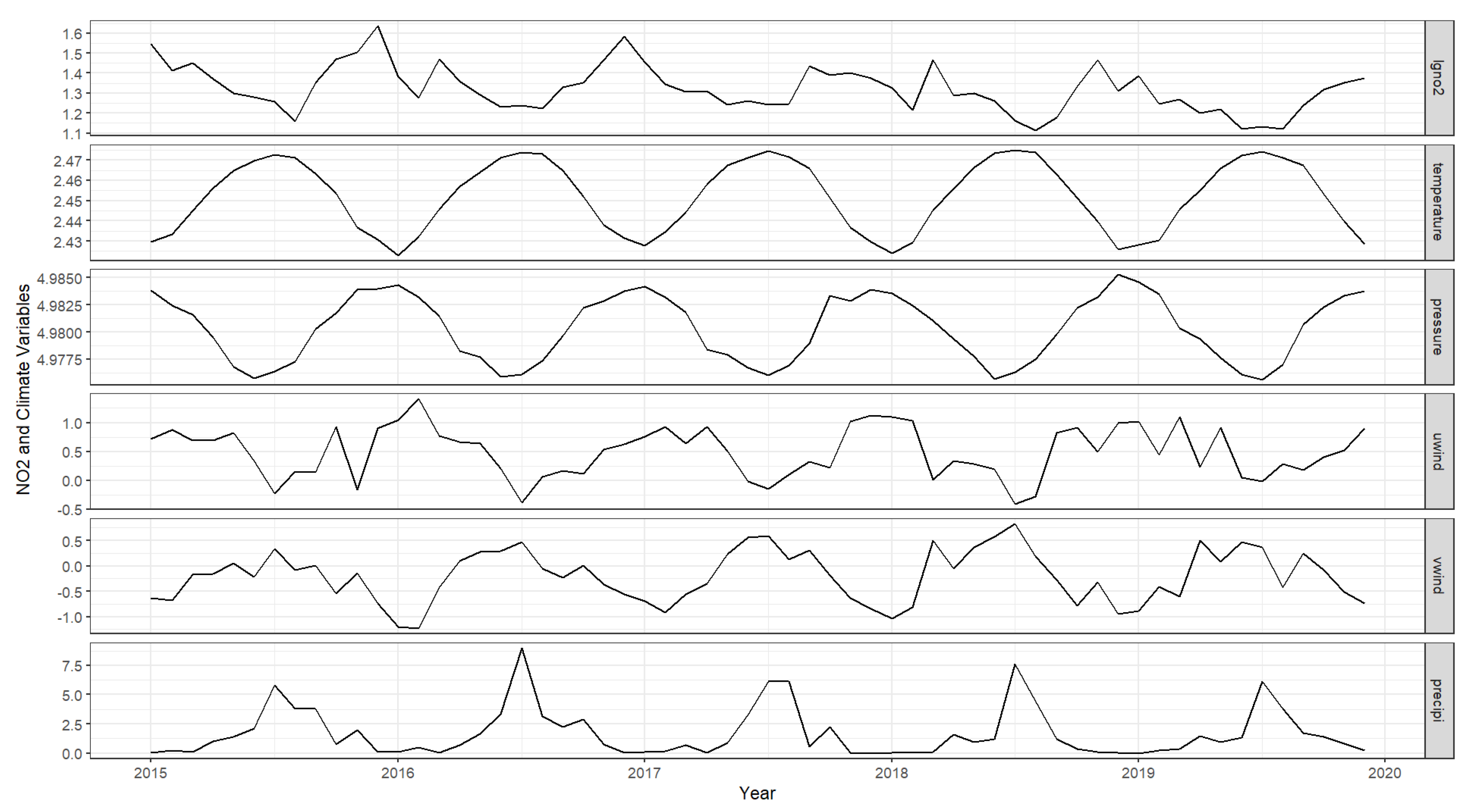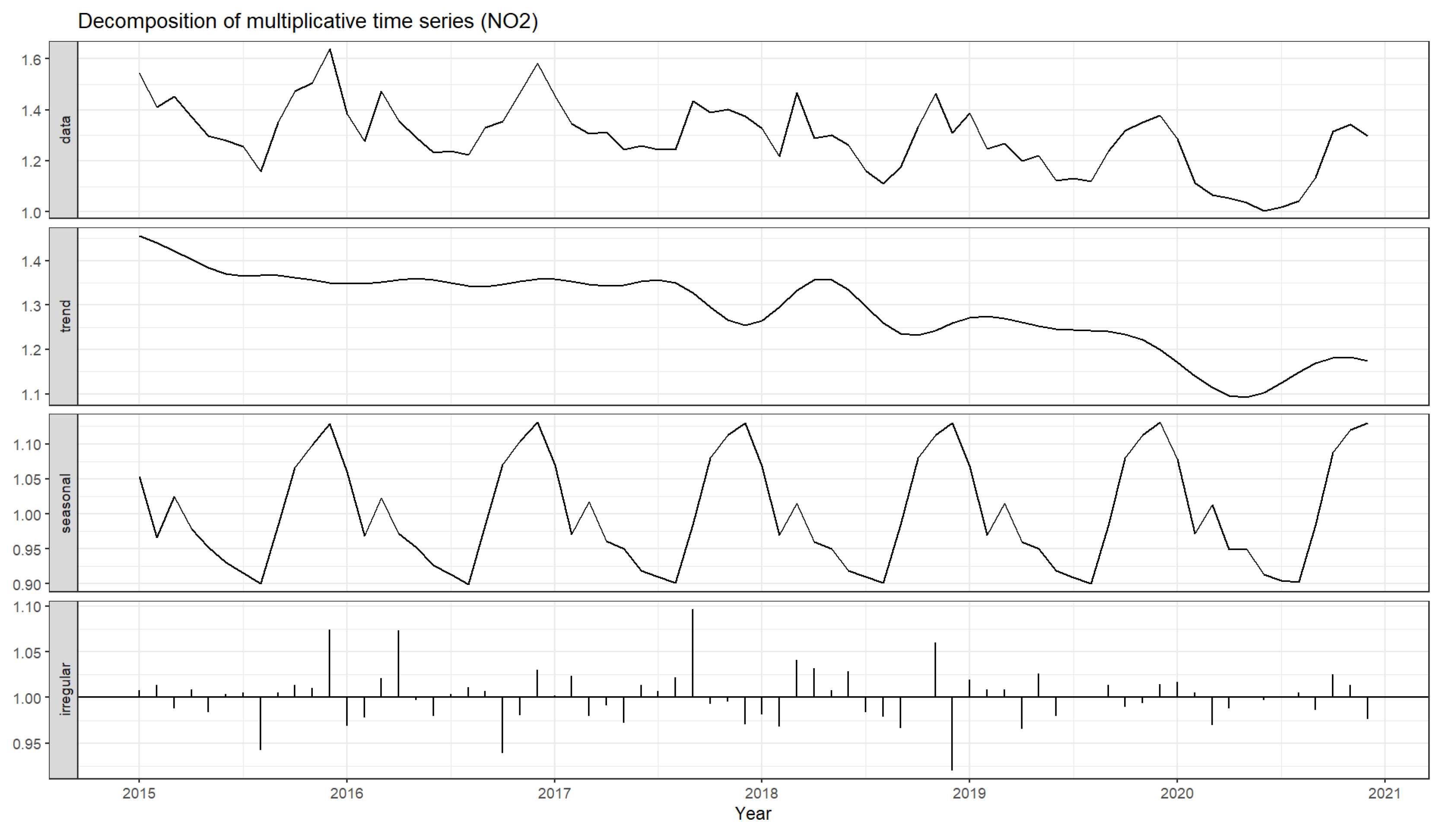We simulated daily and monthly data, respectively, and found that the R² of monthly data (R² = 0.51) performed better than the daily data fitting results (R² = 0.34); however, the model fitting results were not good enough for our prediction goals. Combined with the X11 time series decomposition model, it was further found that the climate data itself exhibits certain seasonal components which are mainly of a cyclical nature, as can be seen from Figure 3; this was especially evident with the monthly data. We therefore defined a trend term and seasonal dummy term for the multiple linear regression model in order to conduct the time-series prediction. The results showed that the monthly data fitting result has a better performance than previous experiments (R²=0.80).

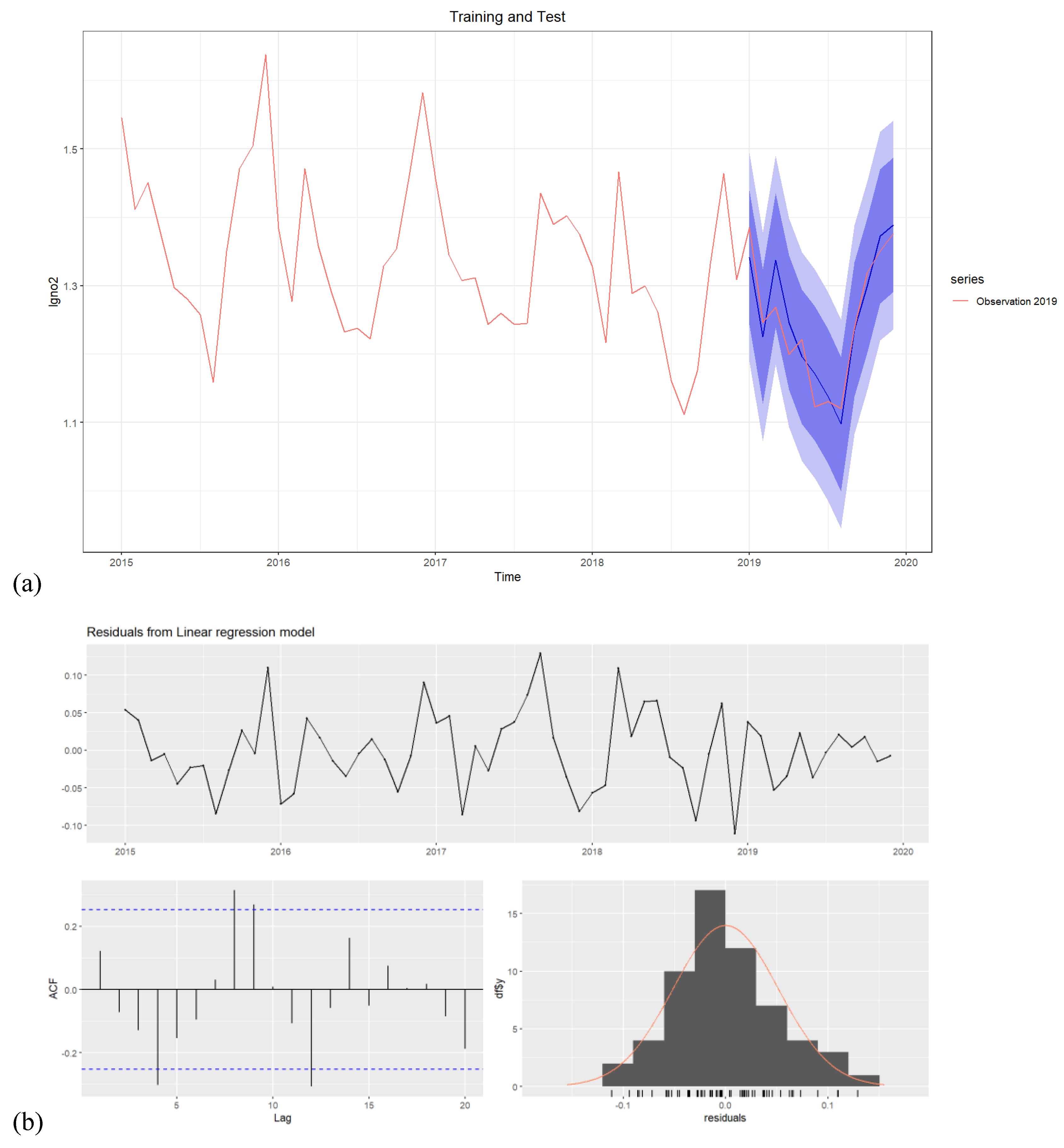
Since we used historical time-series data, the best way of validation is to use historical data 2015-2018 as training data for prediction, and to use 2019 observation data as verification (testing) data to compare that with the expected value from the model prediction results for 2019. The comparison results show that the overall accuracy reaches 97.71%. Figure 7 shows the validation results, and it fits well.

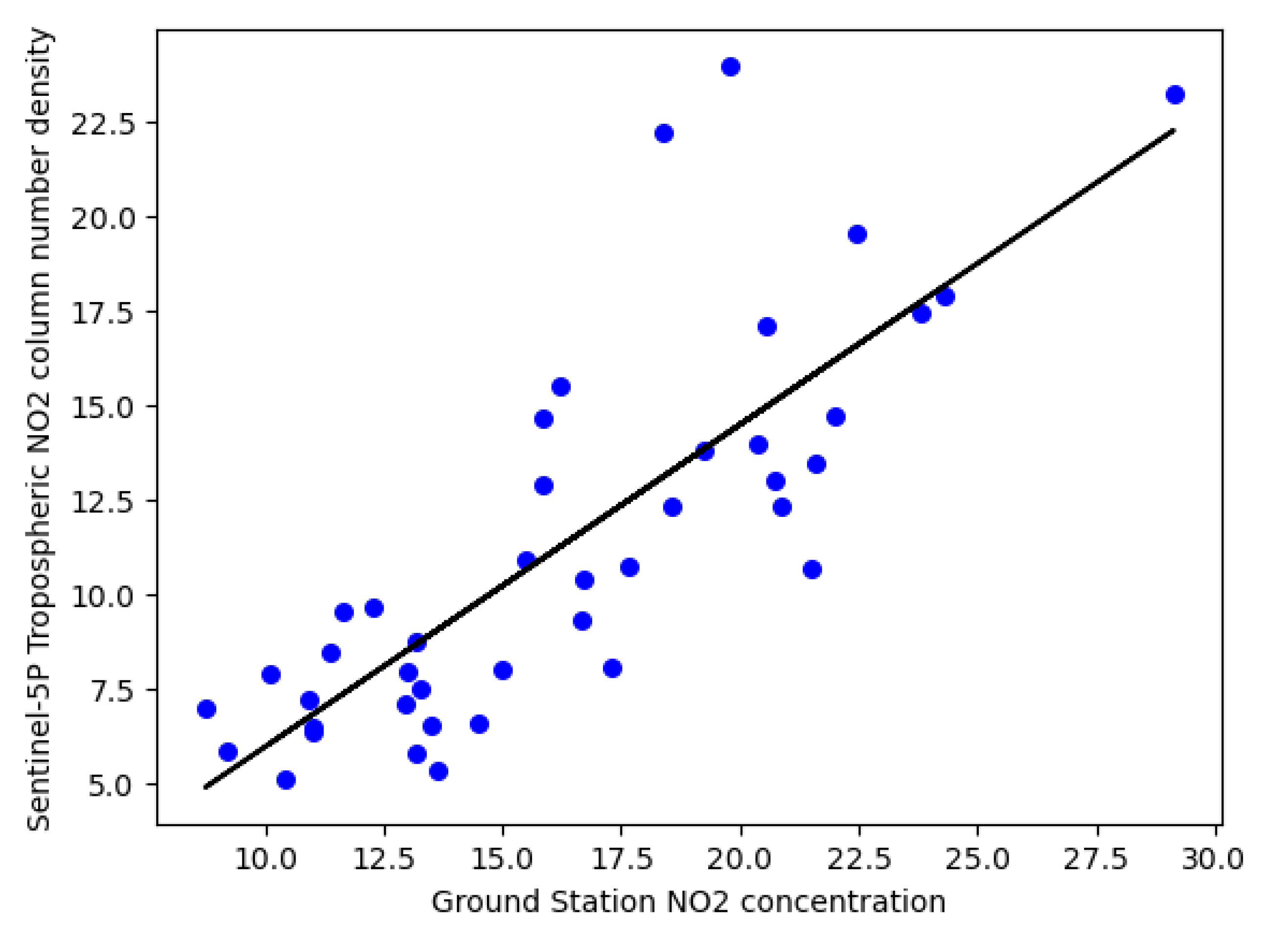
Additionally, this study verified that the satellite data well comply with the ground data by applying a linear regression model. Although different instruments/sensors were used to observe NO₂ levels, the trend changes observed were relatively consistent and significantly correlated (R² = 0.65), as the Figure 8 shown.

6. Conclusion and Discussion

In this study, we employed time-series decomposition and regression-prediction models to evaluate the effects of COVID-19 different containment policies on NO₂ anomalies in Beijing, China. Unlike most previous studies, we detected the effects from seasonality and a long-term downward trend on NO₂ changes and excluded them for analysis. This model design aimed to identify the specific effects due to lockdown measures. The combination of historical ground-based data with satellite datasets enables a more comprehensive evaluation of NO₂ anomalies than monitoring with a single source, by leveraging the strengths of both monitoring datasets. 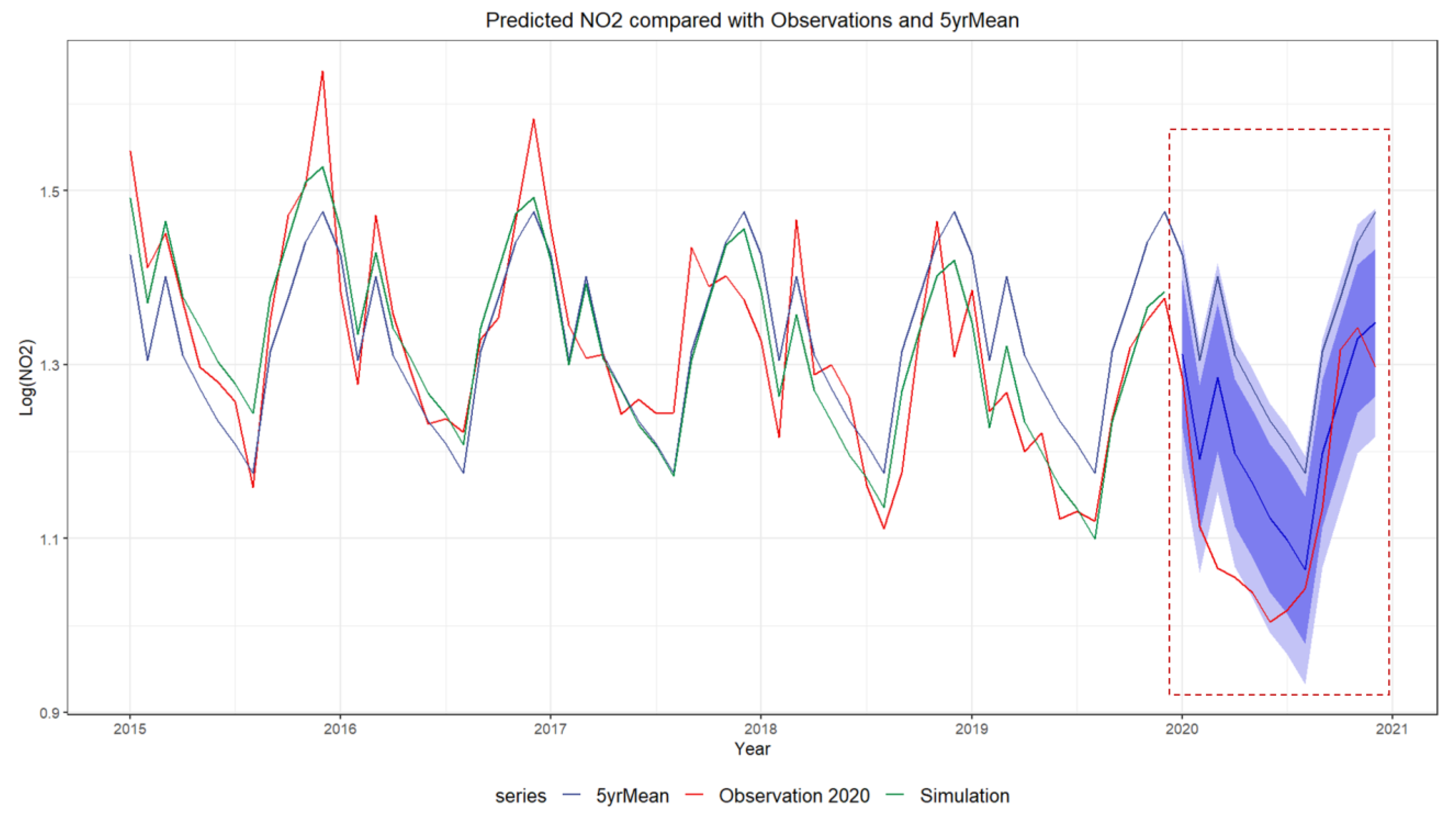This study also verified a well-correlated relationship between these two measurements despite variations in resolutions and types, being consistent with previous studies [25,26].The results showed that observed changes exceeded expectations, with NO₂ decreasing by -6.08% on average every year, and as much as by -17.04% (95% CI, -7.71%~ -24.67%, p < 0.001) in March 2020 when the strictest lockdown measures were in place. Taking the 5-year average level as a baseline, our results show a reduction of 14.10% due to COVID-19 policy measures. Compared with existing research, it is significantly less than the 30%~40% reduction suggested in [9,11] at the city level; but the value is more close to the national average level by 6% [5] though the spatial-temporal records has differences between national- and regional-scale. Therefore, our results suggested that the air quality policies and the local context should not be ignored when assessing the impacts of COVID-19 policies on changes in pollutant levels: beware of exaggerating the effects of the COVID-19 restrictions on NO₂ anomaly. Meanwhle, the combination of historical ground-based data with satellite datasets used in this study, enables a more comprehensive evaluation of NO2 anomalies than monitoring with a single source, by leveraging the strengths of both monitoring datasets. This study verified a well-correlated relationship between these two measurements despite variations in resolutions and types, being consistent with previous studies [25,26].

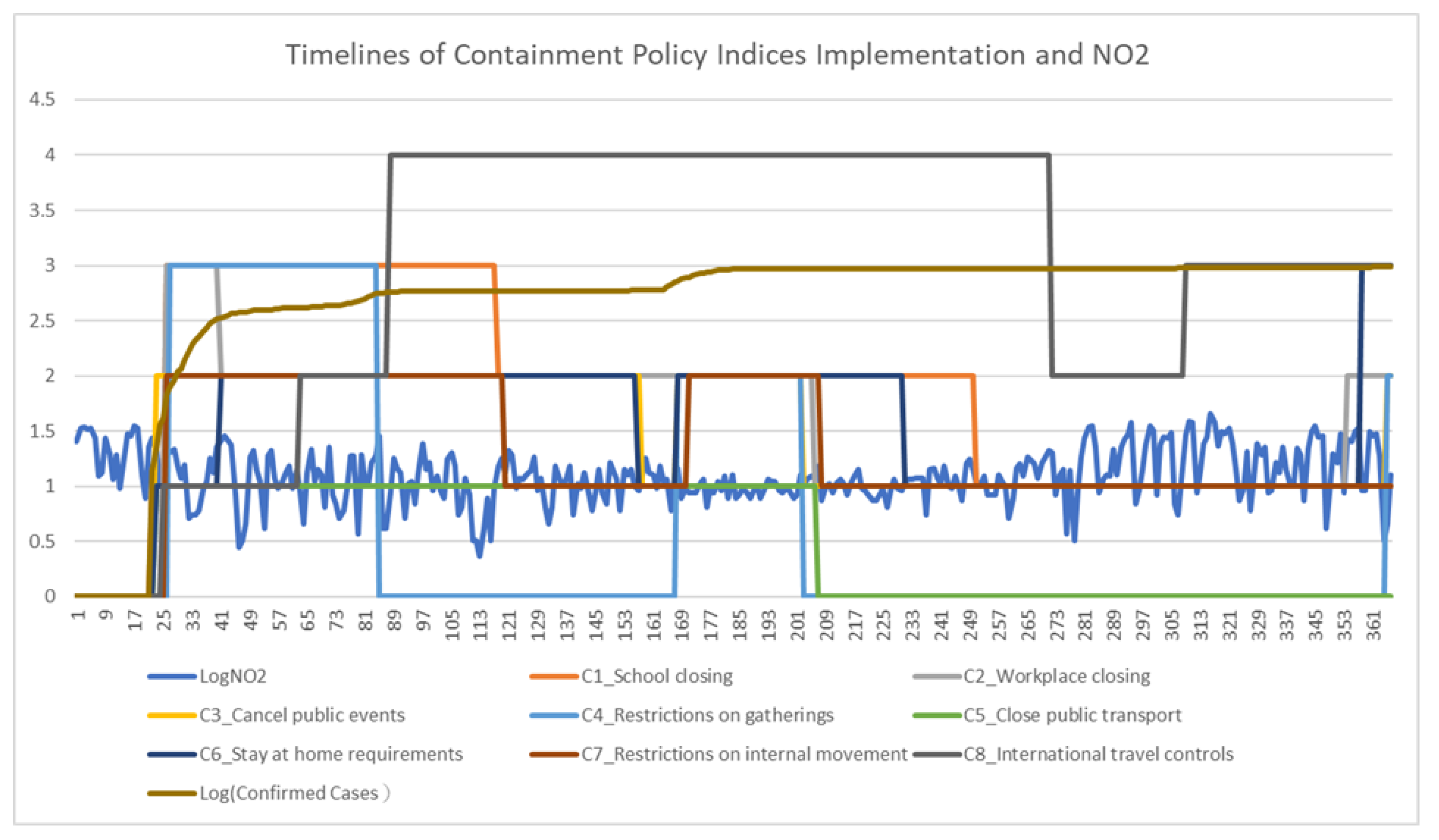
Beyond the effects of policies on NO₂ anomalies widely discussed in many studies [7,8,18], the main novelty and contributions lied in that this study succeed to tell the difference of human activity containment and quantify their contributions to NO₂ anomalies. The top three measures showing dominant effects were C2 “Workplace closure”, C5 “Restricted public transport usage”, and C1 “School closure”, accounting for 54.8%, 52.3%, and 46.4%, respectively. These three dominant policies were respectively linked to restrictions on commuting activities, transportation, and education activities, which were likely to mitigate traffic congestion pressures in this city. By analyzing the contributions of different behavioral constraints to the NO₂ anomalies, we can speculate and reflect on the problems of urban structure and spatial development imbalance in Beijing, that is, the mismatch of employment and housing (determined by commuting patterns), educational inequality and the long-term unsolved congestions, as discussed in previous studies [32,33]. This convincing evidence influenced the top three corresponding restriction policies; in other words, promoting the transformation of urban spatial structure will effectively alleviate air pollution. Now we have the chance to boost the urban shift to environmental sustainability goals, as cities have become more flexible and open to change than in the past in regard to urban planning and environmental management for post-pandemic recovery.

Information about factors which reduce NO₂ emissions during COVID-19 can be helpful in designing policy responses. As seen in this study, the restrictions on human activities, especially those related to transport, played a dominant role in the observed reduction of NO₂. By removing seasonal and trend impacts, the study revealed that NO₂ levels rebounded in the second half of 2020, especially in October and November, with peaks appearing in November that were earlier than in previous years (higher than expected according to the natural cycle). This suggests that the government’s recovery policies, for example to stimulate production activities, should also take into consideration the “retaliatory” emissions. This study is expected to help decision-makers to identify the effects and sensitivity of NO₂ to different policy responses, thereby allowing them to make more precise policies which balance air pollution control and measures to support post-COVID-19 recovery. We have identified the dominant policies and assessed their corresponding magnitudes of influence at the urban-scale level. This evidence may help other regions to examine the impact of their own policies.

This study focuses on evaluating the effects of pandemic restrictions on NO₂ anomalies, it also has some limitations. One is that the forecast of atmospheric trace gases is a complex task which requires expert knowledge in atmospheric sciences. This calls for greater cooperation between researchers in different fields in future. Furthermore, the study used monthly average data to detect NO₂ anomalies during COVID-19 and the model results were well-fitted, while the analysis and simulations for daily changes in NO₂ requires more complex models which can handle a 5-year time scale or even longer, as well as the effects of emerging events, climate change and other uncertainties. Some less obvious potential sources of pollution should also be given more attention. For example, telecommuting decentralized office activities and reduced travel activities, but stay-at-home orders are likely to have increased household consumption of energy. Another consideration is whether less usage of public transport will increase the demand for private cars and generate more pressure on air quality. Next, comparison studies between countries will be conducted to explore different policy-driven forces, and the applications of these methodology may further examine the variability over regions and time. It would also be useful to fine-tune these methods to assess the policy sensitivity of other types of air pollutants.

The combination of historical ground-based data with satellite datasets enables a more comprehensive evaluation of NO₂ anomalies than monitoring with a single source, by leveraging the strengths of both monitoring datasets. Ground station monitoring offers more accurate in localized measurements of NO₂ concentrations, but it is limited in its coverage of broader geographic areas. Conversely, satellite monitoring has the capability to cover larger areas, reflecting heterogeneity in spatial distribution but it has a relatively less precise localized monitoring. By a more thorough evaluation of NO₂ anomalies was evaluated, in particular, interpreting the relationship to various policy-induced restrictions and their impact on urban structure. This is supported by previous studies [25,26] as well as the validation of this study, which shows that these two measurements have a well-correlated relationship despite variations in resolutions and types.

Author Contributions

Conceptualization and methodology: Jing Kang and Bailing Zhang. Data analysis and visualization– Jing Kang and Bailing Zhang. Writing original draft –Jing Kang and Bailing Zhang. Review and editing: Jing Kang, Junyi Zhang and Anrong Dang.

Funding

This research was supported by the Key Project of the National Natural Science Foundation of China (Grant No. 52130804), the USDOT Tier 1 University Transportation Center “Cooperative Mobility for Competitive Megaregions” (CM2) (USDOT Award No. 69A3551747135) and by the Center for the Planetary Health and Innovation Science, Hiroshima University.

Data Availability Statement

the data source and processing platform have been mentioned in Section 2. People can download the data from the link that shared in this paper.

Acknowledgments

We are very grateful to the Beijing Environmental Protection Monitoring Center and World Air Quality Index Project, the Copernicus Program Sentinel-5P developed by European Space Agency, to Oxford University's COVID-19 Government Response Tracker Project and to Google Earth Engine for providing the open data and cloud computing platform in this research. We owe a debt of gratitude to Dr. Zhongjie Lin of University of Pennsylvania for his inputs to this paper from urban spatial planning perspective. We thank Jenny Yamamoto for English editing support.

Conflicts of Interest

The authors declare no conflict of interest.

Appendix A

Figure A1. The timeline and degree/intensity of implementation of C1-C8 series policies related to containment of human activities (eight categories, 0-4 levels); and the daily NO₂ observation data curve (the logarithm of NO₂ was taken to ensure the stability of the mean square error). It was superimposed on the change curve of the number of infected people and NO₂ level to reflect the dynamic adjustments of policies.

References

Van der A, R. J.; Eskes, H.J.; Boersma, K.F.; Noije van, T.P.C.; Roozendael van, M.; Smedt de, I.; Peters, D.H.M.U.; Meijer, E.W. Trends, seasonal variability and dominant NOx source derived from a ten year record of NO₂ measured from space. JGR Atmospheres. 2008, 113. [Google Scholar] [CrossRef]
Liu, J.; Mauzerall, D.L.; Chen, Q.; Zhang, Q.; Song, Y.; Peng, W.; Klimont, Z.; Qiu, X.H.; Zhang, S.Q. ; Hu, Min.; Lin, W.L., Smith, K.R., Eds.; Zhu, Tong. Air pollutant emissions from Chinese households: A major and underappreciated ambient pollution source. PNAS. 2016, 113(28), 7756-7761. [Google Scholar] [CrossRef]
World Health Organization. Global surveillance, prevention and control of chronic respiratory diseases: a comprehensive approach. 2007. Available online: http://apps.who.int/iris/bitstream/handle/10665/43776/9789241563468_eng.pdf;jsessionid=530B0DB46C92CCFDA8CACEC5843BE024?
Ogen, Y. Assessing nitrogen dioxide (NO₂) levels as a contributing factor to coronavirus (COVID-19) fatality. Sci. Total Environ. 2020, 726, 138605. [Google Scholar] [CrossRef] [PubMed]
Xing, X.F.; Xiong, Y.K.; Yang, R.P.; Wang, R.; Wang, W.B.; Kan, H.D.; Lu, T.; Li, D.S.; Cao, J.J.; Peñuelas, J.; Ciais, P.; Bauer, N.; Boucher, O.; Balkanski, Y.; Hauglustaine, D.; Brasseur, G.; Morawska, L.; Janssens, I.A.; Wang, X.R.; Sardans, J.; Wang, Y.J.; Deng, Y.F.; Wang, L.; Chen, J.M.; Tang, X.; Zhang, R.H. Predicting the effect of confinement on the COVID-19 spread using machine learning enriched with satellite air pollution observations. PNAS. 2021, 118(33), e2109098118. [Google Scholar] [CrossRef] [PubMed]
European Environment Agency. Urban sustainability in Europe - Post-pandemic drivers of environmental transitions. 2022. Available online: https://www.eea.europa.eu/publications/urban-sustainability-drivers-of-environmental.
Cooper, M.J.; Randall, V.M.; Melanie, S.; Hammer, P.F.; Levelt, P.V.; Lok, N.L.; Nickolay, A.K.; Jeffrey, R.B.; Chris, A.M. Global fine-scale changes in ambient NO₂ during COVID-19 lockdowns. Nature. 2022, 601(7893), 380–387. [Google Scholar] [CrossRef] [PubMed]
Venter, Z.S.; Aunan, K.; Chowdhury, S. ; Lelieveld, Jos. COVID-19 lockdowns cause global air pollution declines. PNAS. 1898. [Google Scholar] [CrossRef]
Al-qaness, M.A.; Hong, F.; Ahmed, A.; Ewees, D. Yousri.; Mohamed A.E. Improved ANFIS model for forecasting Wuhan City Air Quality and analysis COVID-19 lockdown impacts on air quality. Environ. Res. 2021, 194, 110607. [Google Scholar] [CrossRef] [PubMed]
Kazakos, V.; Taylor, J.; Luo, Z.W. Impact of COVID-19 lockdown on NO₂ and PM_2.5 exposure inequalities in London, UK. Environ. Res. 2021, 198, 111236. [Google Scholar] [CrossRef] [PubMed]
Tzortziou, M.; Kwong, C.F.; Goldberg, D.; Schiferl, L.; Commane, R.; Abuhassan, N.; Szykman, J.J.; Valin, L.C. Declines and peaks in NO₂ pollution during the multiple waves of the COVID-19 pandemic in the New York metropolitan area. Atmos. Chem. Phys. 2022, 22(4), 2399–2417. [Google Scholar] [CrossRef] [PubMed]
Damiani, A.; Irie, H.; Belikov, D.; Kaizuka, S.; Hoque, H.M.S.; Cordero, R.R. Peculiar COVID-19 effects in the Greater Tokyo Area revealed by spatiotemporal variabilities of tropospheric gases and light-absorbing aerosols. Atmos. Chem. Phys. 2022, 22(18), 12705–12726. [Google Scholar] [CrossRef]
Zhao, X.Y.; Fioletov, V.; Alwarda, R.; Su, Y.; Griffin, D.; Weaver, D.; Strong, K.; Cede, A.; Hanisco, T.; Tiefengraber, M.; McLinden, C.; Eskes, H.; Davies, J.; Ogyu, A.; Sit, R.; Abboud, I.; Lee, S.C. Tropospheric and Surface Nitrogen Dioxide Changes in the Greater Toronto Area during the First Two Years of the COVID-19 Pandemic. Remote Sens. 2022, 14(7), 1625. [Google Scholar] [CrossRef]
Etchie, T.O.; Ayotunde, T.E.; Jauro, A.; Pinker, R.T.; Swaminathan, N. Season, not lockdown, improved air quality during COVID-19 State of Emergency in Nigeria. Sci. Total Environ. 2021, 768, 145187. [Google Scholar] [CrossRef]
Jakob, A.; Hasibuan, S.; Fiantis, Dian. Empirical evidence shows that air quality changes during COVID-19 pandemic lockdown in Jakarta, Indonesia are due to seasonal variation, not restricted movements. Environ. Res. 2022, 208, 112391. [Google Scholar] [CrossRef]
Shakil, M.H.; Munim, Z.H.; Tasnia, M.; Sarowar, S. COVID-19 and the environment: A critical review and research agenda. Sci. Total Environ. 2020, 745, 141022. [Google Scholar] [CrossRef]
Misra, P.; Takigawa, M.; Khatri, P.; Dhaka, S.K.; Dimri, A.P.; Yamaji, K.; Kajino, M.; Takeuchi, W.; Imasu, R. ; Nitta, Kaho.; Patra, P.K.; Hayashida, S. Nitrogen oxides concentration and emission change detection during COVID-19 restrictions in North India. Sci. Rep. 9800. [Google Scholar] [CrossRef]
Li, Y.; Li, M.M.; Rice, M.; Yang, C.W. Impact of COVID-19 containment and closure policies on tropospheric nitrogen dioxide: A global perspective. Environ Intern. 2022, 158, 106887. [Google Scholar] [CrossRef] [PubMed]
UN Environment. A Review of 20 Years’ Air Pollution Control in Beijing, United Nations Environment Programme, Nairobi, Kenya. 2019. Available online: https://www.unep.
Feng, Y.Y.; Ning, M.; Lei, Y.; Sun, Y.; Liu, W.; Wang, J. Defending blue sky in China: Effectiveness of the “Air Pollution Prevention and Control Action Plan” on air quality improvements from 2013 to 2017. J. Environ. Manage. 2019, 252, 109603. [Google Scholar] [CrossRef] [PubMed]
Kang, J.; Kong, H.; Lin, Z.J.; Dang, A.R. Mapping the dynamics of electric vehicle charging demand within Beijing's spatial structure. Sustain. Cities Soc. 2022, 76, 103507. [Google Scholar] [CrossRef]
Fu, F.; Purvis-Roberts, K.L.; Williams, B. Impact of the COVID-19 Pandemic Lockdown on Air Pollution in 20 Major Cities around the World. Atmosphere. 2020, 11, 1189. [Google Scholar] [CrossRef]
Dark, S.J. ; Danielle, Bram. The modifiable areal unit problem (MAUP) in physical geography. Prog Phys Geog. [CrossRef]
Gong, P.; Chen, B.; Li, X.; Liu, H.; Wang, J.; Bai, Y.; Chen, J.; Chen, X.; Fang, L.; Feng, S.; Feng, Y.; Gong, Y.; Gu, H.; Huang, H.; Huang, X.; Jiao, H.; Kang, Y.; Lei, G.; Li, A. ;... Xu, B. Mapping essential urban land use categories in China (EULUC-China): preliminary results for 2018. Sci. Bull. [CrossRef]
Lorente, A.; Boersma, K.F.; Eskes, H.J.; Veefkind, J.P.; Geffen van, J.H.G.M.; Zeeuw de, M. B.; Denier van der gon, H.A.C.; Beirle, S.; Krol, M.C. Quantification of nitrogen oxides emissions from build-up of pollution over Paris with TROPOMI. Sci. Rep. 2019, 9(1), 20033. [Google Scholar] [CrossRef]
Griffin, D.; Zhao, X.Y.; McLinden, C.A.; Boersma, F.; Bourassa, A.; Dammers, E.; Degenstein, D.; Eskes, H.; Fehr, L. ; Fioletov,Vitali. High-resolution mapping of nitrogen dioxide with TROPOMI: First results and validation over the Canadian oil sands. Geophys Res Lett. 1049. [Google Scholar] [CrossRef]
Dabbour, L.; Eman, A.; Mohammad, H. Effect of climatology parameters on air pollution during COVID-19 pandemic in Jordan. Environ. Res. 2021, 202, 111742. [Google Scholar] [CrossRef]
Zha, H.; Zhang, Y.X.; Zhou, H.; Wang, L.J.; Zhang, Z.H.; Tan, Z.J.; Deng, L.M.; Hale, T. Chinese Provincial Government Responses to COVID-19, Version 2. Blavatnik School of Government Working Paper. 2022. Available online: http://www.bsg.ox.ac.uk/covidtracker.
Wang, X.Z.; Smith, K. ; Hyndman, Rob. Characteristic-Based Clustering for Time Series Data. Data Min Knowl Discov. 2006, 13 (3), 335-364. [CrossRef]
Wang, J.F.; Li, X.H.; Christakos, G.; Liao, Y.L.; Zhang, T.; Gu, X.; Zheng, X.Y. Geographical Detectors-Based Health Risk Assessment and its Application in the Neural Tube Defects Study of the Heshun Region, China. Int J Geogr Inf Sci. 2010, 24(1), 107–127. [Google Scholar] [CrossRef]
Wang, J.F.; Zhang, T.L.; Fu, B.J. A measure of spatial stratified heterogeneity. Ecol. Indic. 2016, 67, 250–256. [Google Scholar] [CrossRef]
Lu, M.; Sun, C.; Zheng, S. Congestion and pollution consequences of driving-to-school trips: A case study in Beijing. Transport Res D-Tr E.. 2017, 50, 280–291. [Google Scholar] [CrossRef]
Zhang, M.; He, S.; Zhao, P. Revisiting inequalities in the commuting burden: Institutional constraints and job-housing relationships in Beijing. J Transp Geogr. 2018, 71, 58–71. [Google Scholar] [CrossRef]

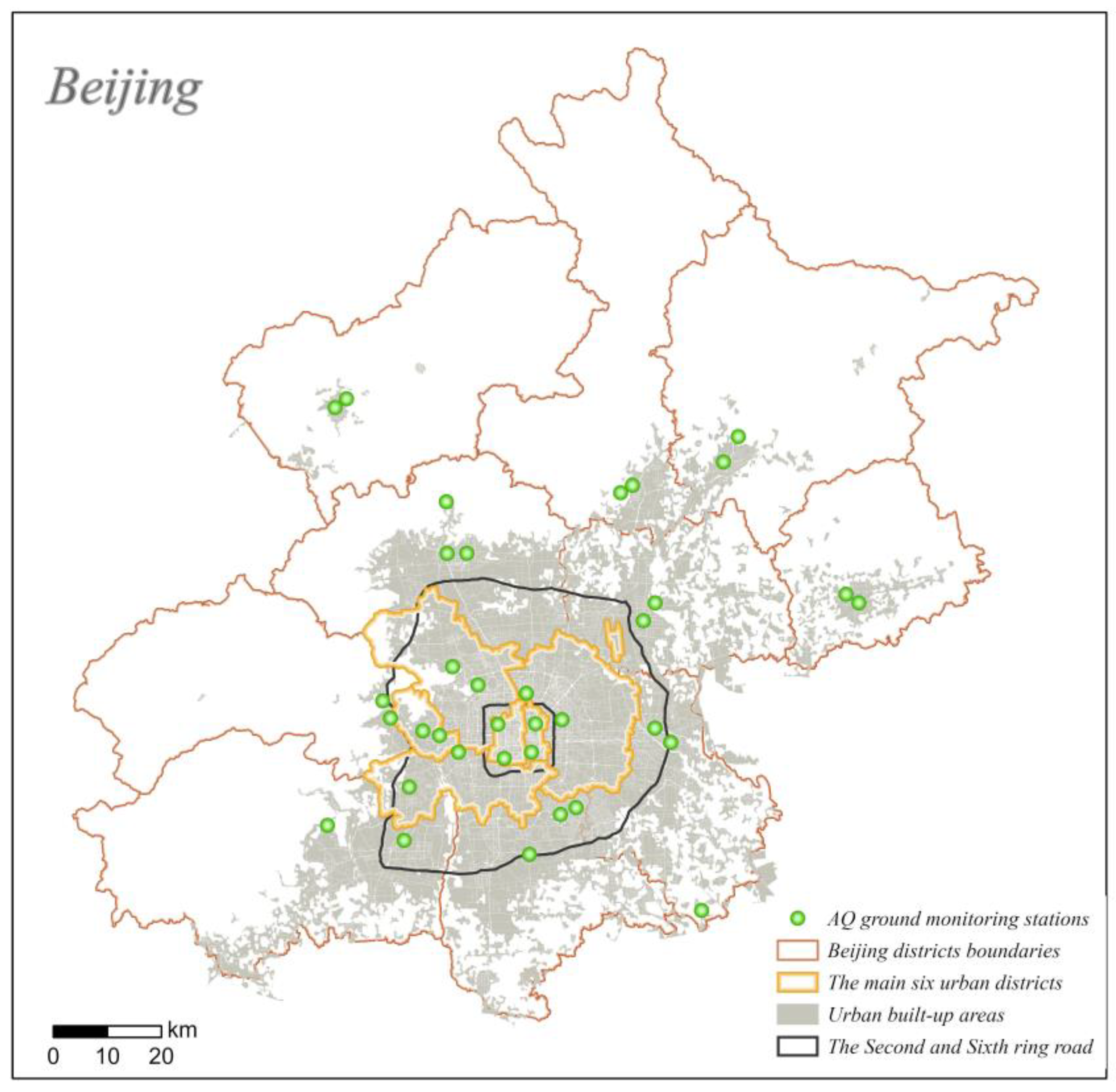
Figure 1. Map of study area, overlay with Air Quality (AQ) ground-station distributions (as the green points). The built-up areas come from [24] represent the urban extent in general; The ring roads witnessed the development and expansion of the city that can help with understanding the urban, suburban, and rural areas of the city. In particular, the areas within the second ring road are the historic urban centers, the sixth ring road is currently the outermost ring road.

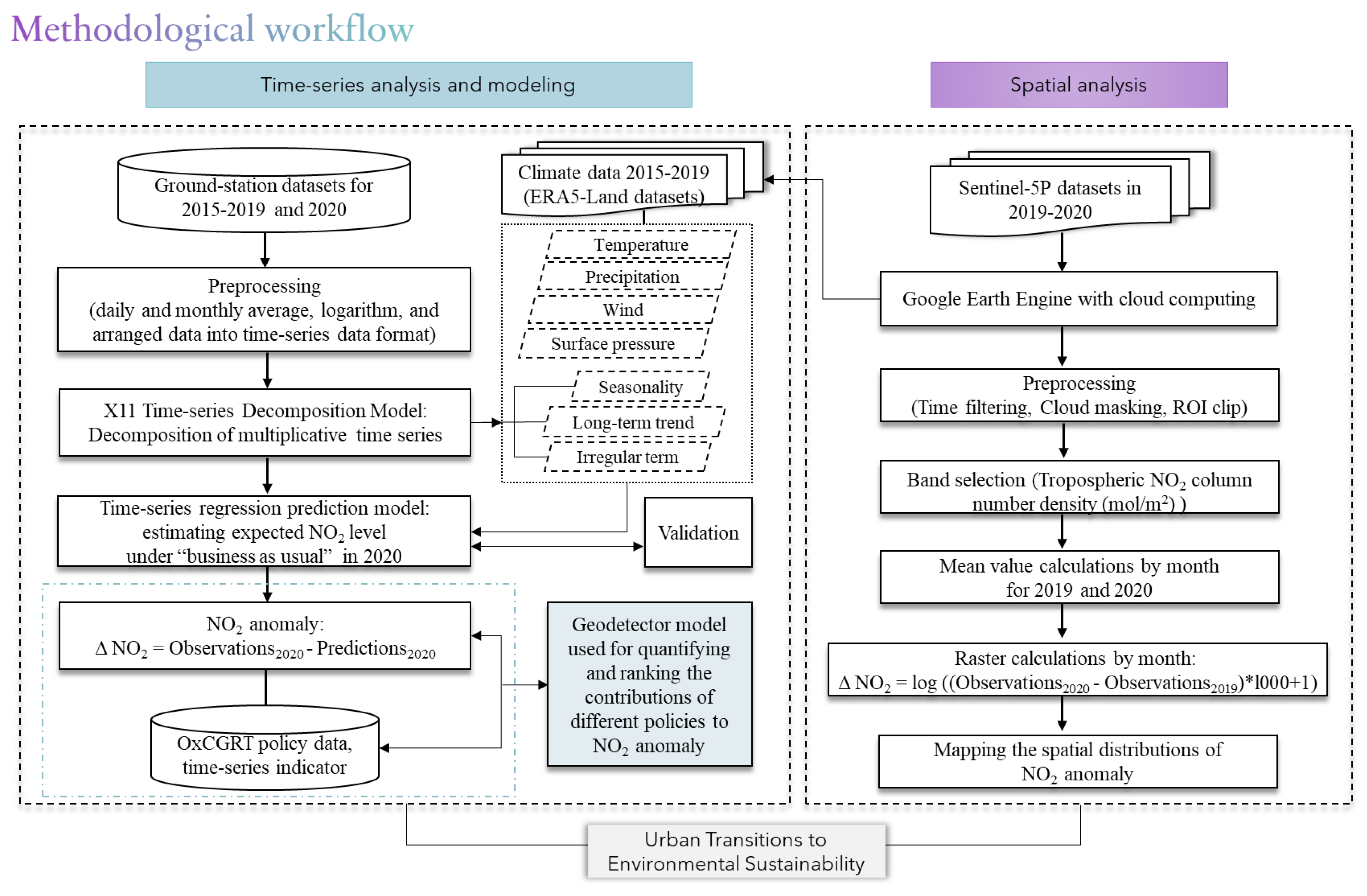
Figure 2. Overview of the methodological workflow.

Figure 3. Initial analysis graph based on characteristics of monthly average of NO₂ emissions from 2015 to 2019 and meteorological factors (temperature, precipitation, wind, surface pressure) in Beijing China. lgno2 represents the logarithm of NO₂, uwind represents Eastward component of the 10m wind, vwind represents Northward component of the 10m wind, precipi represents precipitation here.

Figure 4. Decomposition of multiplicative time series of observed NO₂ data from 2015 to 2020 based on ground station data. The top graph is the original observed NO₂ data, consisting of the trend, seasonal and irregular components (the three-bottom terms).

Figure 5. Comparison between observation and expectation (prediction line). The multiple linear regression model prediction line (blue line with buffer range) is shown as the base map (the light blue buffer is the 95% confidence interval), superimposing on the previous 5-year average as the reference baseline (grey blue line namely 5yrMean as shown) and the regression simulation fitting curve (light grey line), compared to the actual observed value (red line).

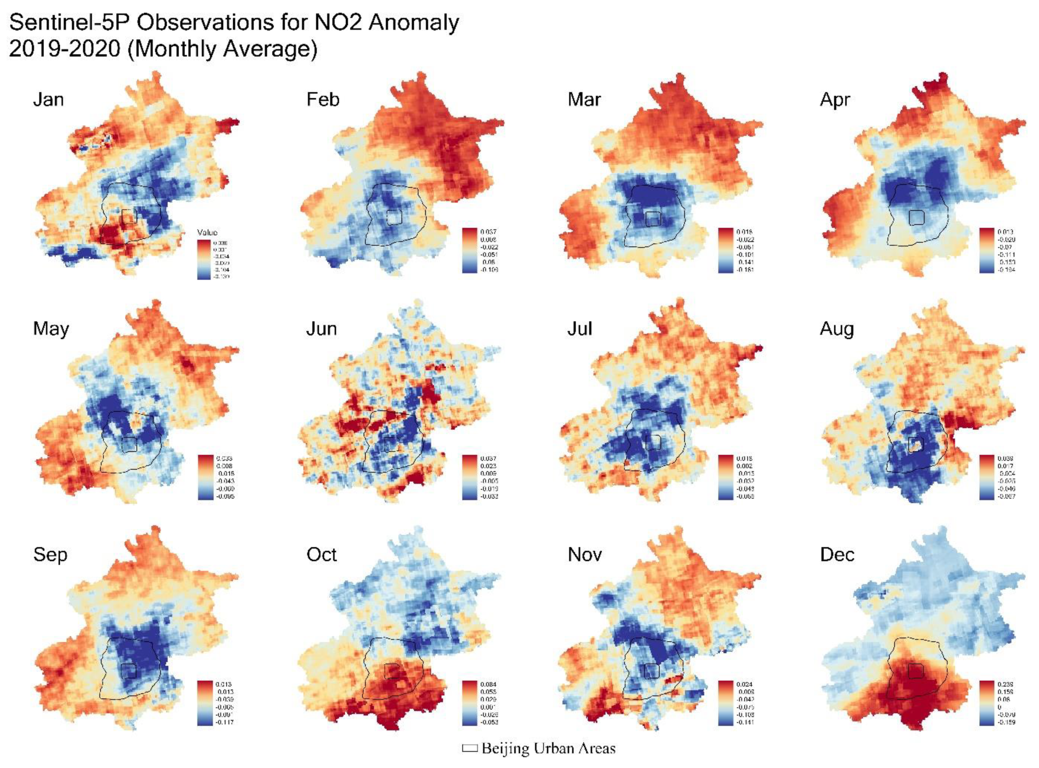
Figure 6. Changes of NO₂ levels comparing the years 2019 and 2020, using the monthly average data of tropospheric NO₂ column number density (mol/m²) from Sentinel 5P. The changes or differences are calculated by taking 2020 levels minus the same period in 2019. The satellite observation data show the spatial heterogeneity (different spatial distributions) of NO₂ levels at 1 km spatial resolution.

Figure 7. Model performance assessment results and the residuals analysis of the time-series multi-linear regression prediction model. (a) shows the validation results in terms of using the data for 2015-2018 for training and the 2019 observation data for comparison. (b) shows a time plot, the ACF and the histogram of the residuals from the multiple regression model fitted to the NO₂ data, as well as the Breusch-Godfrey test for jointly testing up to 16th order autocorrelation. The histogram shows that the residuals seem to be slightly skewed, which may also reflect the coverage probability of the prediction intervals.

Figure 8. The correlation between the ground station NO₂ concentration and Satellite observed tropospheric NO₂ column number density. The analysis was based on 42 monthly average data from July 2018 to December 2021 as the NO₂ column was released by Sentinel 5P since July 2018.

Table 1. Comparison of results between observation and expected trend.

Month	Predicted 2020 (95% CI)	Observ 2019	5-yr baseline	Observ 2020	Predicted 2020- Observ 2019	Observation -Prediction 2020	Observation 2020-2019	Observation-5yr-baseline
Jan	1.312±0.13	1.385	1.426	1.285	-5.32%	-2.07%	-7.25%	-9.93%
Feb	1.192±0.13	1.247	1.305	1.114	-4.42%	-6.52%	-10.63%	-14.65%
Mar	1.285±0.13	1.268	1.401	1.066	1.32%	-17.04%	-15.95%	-23.92%
Apr	1.198±0.13	1.200	1.310	1.056	-0.10%	-11.92%	-11.97%	-19.45%
May	1.163±0.13	1.221	1.272	1.038	-4.79%	-10.78%	-15.01%	-18.42%
Jun	1.124±0.13	1.123	1.235	1.004	0.07%	-10.61%	-10.58%	-18.67%
Jul	1.098±0.13	1.131	1.209	1.018	-2.88%	-7.33%	-9.98%	-15.81%
Aug	1.064±0.13	1.120	1.175	1.043	-5.05%	-1.99%	-6.91%	-11.26%
Sep	1.198±0.13	1.238	1.315	1.135	-3.23%	-5.30%	-8.32%	-13.73%
Oct	1.266±0.13	1.320	1.377	1.317	-4.10%	+4.05%	-0.19%	-4.36%
Nov	1.330±0.13	1.351	1.441	1.342	-1.56%	+0.94%	-0.66%	-6.84%
Dec	1.348±0.13	1.376	1.476	1.297	-2.05%	-3.82%	-5.77%	-12.13%
Average Reduced by			-2.68%			-6.03%	-8.60%	-14.10%

* observ represents observation. observation minus prediction is comparison for 2020.

Table 2. q-statistics of different policy factors.

Containment	q	p value	Policy intensity (Sig t test:0.05)
Policy measures	q	p value	0	1	2	3	4
C1 School closing	0.464	0.000	0.028	0.010	0.087^#	0.131	--
C2 Workplace closing	0.548	0.000	0.028	0.015	0.122^#	0.051	--
C3 Cancel public events	0.448	0.000	0.028	0.025	0.119^#	--	--
C4 Restrictions on gatherings	0.148	0.000	0.054	0.091	0.127^#	--	--
C5 Close public transport	0.523	0.000	0.018	0.120^#	--	--	--
C6 Stay at home requirements	0.421	0.000	0.028	0.023	0.116^#	0.044	--
C7 Restrictions on internal movement	0.289	0.000	0.028	0.043	0.120^#	--	--
C8 International travel controls	0.153	0.000	0.028	0.072	0.063	0.020	0.092^#

* Note: the range from 0 to 4 represent the different policy intensity. In general, for example, 0 means no measures;1 represents recommendations; 2~4 refer to different requirements of the policy. The right six column show average NO2 anomaly observed in each sub-stratum under each Ci (i=8). # means this sub-stratum has a statistically significant difference in the average anomaly incidence, having the highest effects on NO2 anomaly compared with others.

Disclaimer/Publisher’s Note: The statements, opinions and data contained in all publications are solely those of the individual author(s) and contributor(s) and not of MDPI and/or the editor(s). MDPI and/or the editor(s) disclaim responsibility for any injury to people or property resulting from any ideas, methods, instructions or products referred to in the content.

© 2023 by the authors. Licensee MDPI, Basel, Switzerland. This article is an open access article distributed under the terms and conditions of the Creative Commons Attribution (CC BY) license (http://creativecommons.org/licenses/by/4.0/).

Copyright: This open access article is published under a Creative Commons CC BY 4.0 license, which permit the free download, distribution, and reuse, provided that the author and preprint are cited in any reuse.

MDPI Initiatives

Important Links

Choose an area of interest and we will send you notifications of new preprints at your preferred frequency.

Disclaimer