
Submitted:
20 March 2023
Posted:
21 March 2023
Read the latest preprint version here
Abstract
Coincident changes in abundance and behavior pose a challenge for interpreting abundance data from monitoring programs. In the San Francisco Estuary, long-term monitoring documented the declines of many species including the anadromous Longfin Smelt (Spirinchus thaleichthys). We identified seasonal patterns in reginal presence of Longfin Smelt through its life cycle using monitoring data and generalized additive modelling. We then investigated the year-to-year variability in the seasonal patterns of presence using functional data analysis (FDA). FDA separated the variability due to population size from variability due to differences in timing of presence. We found that Longfin Smelt have consistent seasonal distribution patterns and that two trawl types were needed to accurately describe those patterns. After accounting for variability due to year-class strength, shifts in the timing of presence were evident in three regions. The most variable period for the upstream regions Suisun Bay and West Delta was for age-0 fish in summer and for the downstream region Central Bay was for age-0 fish in late fall. This manifested as a delay in the typical fall re-occupation of upstream regions that comprise the study area for another monitoring study (Fall Midwater Trawl). Thus, a portion of the recent reductions in Fall Midwater Trawl abundance of Longfin Smelt resulted from changes in behavior rather than a decline in abundance. The presence of multiple monitoring surveys allowed analysis of distribution from one data set to aid interpretation of patterns in abundance from another monitoring survey. This study highlights how identifying portions of the life cycle with the most and least variability in distribution can help inform the types of management strategies that will be most effective. It also illustrates an analytical method that can be used to address the problem of confounded effects of abundance and behavior on patterns in monitoring data.
Keywords:
fish
; functional data analysis
; long-term monitoring
; habitat
; occupancy
; modeling
; California
1. Introduction
Ecological monitoring studies generate data on the status of fish species and communities, and they can serve as a context for interpreting trends in abundance and community structure. These “status and trends monitoring programs” provide essential information for decision-makers and ecosystem managers on the state of a system over time (Reynolds et al. 2016). Long-term ecological monitoring can be especially valuable for making inferences about ecosystem dynamics in systems with non-linear relationships between drivers and the variables of interest (Giron-Nava et al. 2017). Even when monitoring studies are designed for status and trends, they can also provide multiple values such as quantifying ecosystem responses to environmental change, providing data for developing and testing models, and serving as a framework for collaborative research (Lindenmayer et al. 2012).
One example of a very long-running status and trends monitoring enterprise is the suite of monitoring studies conducted by the Interagency Ecological Program for the San Francisco Estuary (IEP; IEP 2022). These studies have documented changes in fish abundance in the San Francisco Estuary (SFE) for several decades, including a substantial loss of pelagic productivity in the SFE in the late 1980s (Kimmerer and Orsi 1996; Kimmerer 2002) and a collapse in the abundance of several fish species in the early 2000s, a phenomenon referred to as the Pelagic Organism Decline (POD; Sommer et al. 2007). Among the POD species is the Longfin Smelt (Spirinchus thaleichthys). Once one of the most abundant pelagic fishes in the estuary (Orsi 1999), Longfin Smelt was likely an important forage fish in the historical SFE. More recently, monitoring programs have documented the decline in Longfin Smelt abundance and helped identify the factors behind it (Rosenfield and Baxter 2007, Thomson et al. 2010). Freshwater outflow or a suite of correlated variables has been and continues to be considered a significant factor in Longfin Smelt abundance in the SFE (Stevens and Miller 1983; Jassby et al. 1995; Kimmerer 2002; Nobriga and Rosenfield 2016; Tamburello et al. 2018), though in the years after the introduction of the overbite clam, Potamocorbula amurensis (aka Corbula amurensis), declines in the copepod Eurytemora affinis and the virtual loss of the mysid Neomysis mercedis as principal food sources had a negative effect on Longfin Smelt abundance (Kimmerer and Orsi 1996; Orsi and Mecum 1996; Kimmerer 2002; Mac Nally et al. 2010; Thomson et al. 2010). Monitoring data were also used to show that adult stock size also exerts a strong influence on abundance of age-0 Longfin Smelt (Nobriga and Rosenfield 2016).
The well-documented declines in fish species in the SFE and other bodies of water may reflect more than simply declining abundance. Changing conditions that reduce abundance may also cause species to change their behavior. Numerous species world-wide have exhibited changes in diet as a result of changes in food availability following the introduction of invasive species. For example, an invasive plant in salt marshes in France caused diet shifts in Sand Gobies and Sea Bass (Laffaille et al. 2005) and an invasive crayfish changed the diet of a Chub in Britain (Wood et al. 2017). In the SFE, the invasion of the overbite clam in the SFE changed the diets of several species (Feyrer et al. 2003). Fish may also change their habitat use as a result of changing conditions. The introduction of the zebra mussel (Dreissena polymorpha) to the Hudson River estuary led to distributional shifts in young-of-the-year pelagic fishes downstream and young-of-the-year shoreline fishes upstream of the zebra mussel zone (Strayer et al. 2004). Northern Anchovy, the dominant planktivore in the SFE, exhibited declines in abundance in upper regions of the estuary after the introduction of the overbite clam and a drastic decline in pelagic productivity within those regions (Kimmerer 2002, 2006); further, because declines did not occur coincidently in the high salinity region of the estuary or the near coastal marine region, they were interpreted as a downstream shift in distribution (Kimmerer 2006). Similarly, a long-term shift by age-0 Striped Bass from pelagic habitats to shoal habitats was also attributed to declines in pelagic food organisms (Sommer et al. 2011a). The endemic, annual planktivore Delta Smelt employs three life history strategies (Bush 2017, Hobbs et al. 2019), one of which, freshwater residency, acts to partially circumvent direct competition from its otherwise near complete distributional overlap with the invasive overbite clam.
The potential for coincident changes in abundance and behavior poses an interesting challenge for interpreting abundance data from monitoring programs. Shifts in distribution or timing of movements might be interpreted as declines in abundance in the absence of sampling a species’ entire range or investigating habitats not sampled by gear used in abundance estimation. In this paper, we investigate whether there is evidence for behavioral plasticity in addition to a decline in abundance for Longfin Smelt in the long-term monitoring record. In the SFE, Longfin Smelt abundance is monitored primarily by two long-term, open water monitoring surveys: the Fall Midwater Trawl Survey (FMWT) and the San Francisco Bay Study (Bay Study; Honey et al. 2004; Rosenfield and Baxter 2007). The FMWT samples only upper estuary regions. It was used to investigate drivers of the POD but was not able to identify any causative factors among those investigated (Thomson et al. 2010, Mac Nally et al. 2010, CDFW and IEP 2017a). Like the FMWT, the Bay Study samples open-water habitats, but unlike the FMWT, the Bay Study samples throughout the range of the Longfin Smelt within the SFE year-round, so it may provide a more comprehensive view of Longfin Smelt use of the SFE (Figure 1).
We developed a statistical model to identify the main temporal patterns in the regional presence of Longfin Smelt, as detected by the San Francisco Bay Study sampling (CDFW and IEP 2017b). The outcome of this modeling is a set of functions that describes the principal seasonal and long-term patterns in distribution by region and age class, which together describe how Longfin Smelt use the SFE throughout their life cycle. Treating the model output as a set of functions allowed us to separate the effects of abundance from the effects of shifting timing on the probability of observing Longfin Smelt in different regions of the SFE. We used this model to examine how the distribution of Longfin Smelt within the SFE changed over time. We also investigated whether long-term changes in Longfin Smelt distribution can be attributed solely to changes in abundance or whether there is evidence for a shift in behavior. Finally, we discuss how changes in the timing and distribution of Longfin Smelt could affect our interpretation of abundance information derived from a geographically limited monitoring program, the FMWT.
2. Methods
2.1. Study species
Longfin Smelt (Spirinchus thaleichthys) is a small (≤150 mm FL), euryhaline, facultatively-anadromous, pelagic fish belonging to the family Osmeridae (true smelts). It is native to coastal waters of the eastern Pacific Ocean and bays and estuaries, ranging from Monterey Bay to Hinchinbrook Island, Prince William Sound, Alaska (Moyle 2002), farther north to Cook Inlet (Moulton 1997) and possibly west to Bristol Bay, Alaska (Gilbert 1895, Dryfoos 1965, Garwood 2017). Both anadromous and resident populations exist at various locations, and the SFE population is anadromous (Dryfoos 1965; Moulton 1974; Rosenfield and Baxter 2007). The SFE population spawns primarily after its second year of life though some occasionally live to spawn after a third year of life (≥130 mm collected in winter showing two complete annuli, plus growth; Levi Lewis, University of California Davis, personal communication, Email July 11, 2022). Spawning takes place in or near freshwater sources during the winter and spring, through the coldest water temperatures of the year; larvae hatch, typically January through April, and initially rear in fresh and low salinity water and then inhabit progressively more saline regions with development during their first year of life (Baxter 1999, Moyle 2002, Dege and Brown 2004, Hobbs et al. 2010, Grimaldo et al. 2017). This downstream summer movement of developing first year fish reverses as water cools late the following fall and winter when some juvenile fish reoccupy the upper estuary. During the following summer, second year Longfin Smelt move downstream en masse; full marine residency (Central Bay and coastal waters) of these age-1 fish during late summer and fall of their second year of life was inferred from catch data (Rosenfield and Baxter 2007). Finally, during late fall and winter of their second year, Longfin Smelt move upstream to tidal fresh and brackish water to spawn (Moyle 2002, Rosenfield and Baxter 2007). The Longfin Smelt of the SFE represent the southern-most reproductive population and appear genetically distinct from other populations, although there is evidence of gene flow from the SFE population northward to the Humboldt Bay and Columbia River populations (Garwood 2017; Saglam et al. 2021). Based in part on its precipitous abundance decline, Longfin Smelt was listed as threatened under the California Endangered Species act in 2009 (OAL 2010) and the U.S. Fish and Wildlife Service (USFSW) proposed listing Longfin Smelt under the U. S. ESA (U.S. Office of the Federal Register 2022).
2.2. Study area
The SFE is comprised of four, large, open-water embayments (South Bay, Central Bay, San Pablo Bay, and Suisun Bay); the confluence of the Sacramento and San Joaquin rivers, also described as the West Delta; and the Sacramento-San Joaquin Delta, which is a network of tidal channels extending east (upstream), and includes remnants of the emergent wetlands that surround these aquatic habitats (Figure 1). The regional descriptors we used were those defined for the Bay Study and except for the West Delta are those also used by Kimmerer (2004). We refer to the embayments and the West Delta as “regions” and “bays” interchangeably to refer to specific embayments within the SFE. In-flowing river water to the SFE comes mainly from the Sacramento River and tributaries in the north and a lesser amount from the San Joaquin River and tributaries in the south; these inflows meet in the Delta and shift direction to flow west. Net flows (i.e. water not used within the Delta for agriculture or exported south) exit the Delta and move successively through Suisun and San Pablo bays, and downstream towards Central Bay and the Golden Gate Bridge, which spans the outlet of the estuary to the Pacific Ocean. Outflow from the Delta becomes more saline as it flows towards the ocean: generally freshwater in the Delta to marine water in Central Bay (Kimmerer 2004). Freshwater tributaries enter each embayment, and some are known to support Longfin Smelt reproduction, particularly during high flow conditions (Lewis et al. 2020).
Patterns of water flow in the SFE are influenced by climate and human water use factors. The SFE experiences a Mediterranean climate: cold wet winters and springs with rain in the valleys and snow in the Sierra Nevada Mountains followed by hot, dry summers and falls. The SFE experiences highly variable and periodically high, uncontrolled outflows during winter and spring followed by less variable, lower, generally controlled outflows in summer and fall (Arthur et al. 1996). Minimum water temperatures in winter and maximums in late summer vary by region within the estuary, but summer-fall temperatures generally follow the pattern of warmer water upstream and cooler downstream (Kimmerer 2004). Historically, river discharge resulted from low elevation rain runoff in winter and snow melt in spring and early summer followed by declining flows through the late fall. Now, reservoirs partially capture high runoff from winter rainfall and spring snow melt to be released as needed through summer and fall for agricultural, municipal, and ecological uses. At the same time, water export facilities capture as much water as they can during high winter and spring flows but can be constrained if protected fishes are detected nearby or are entrained; summer exports can remain relatively high based on availability of uncontrolled runoff and above-normal reservoir storage, but often are reduced responding to lower reservoir storage levels, the need to maintain in-stream and estuarine flow levels and the need to maintain prescribed water quality in the upper SFE (SWRCB 2000).
2.3. Data
We used data collected by the California Department of Fish and Wildlife’s San Francisco Bay Study (Bay Study) monitoring program (CDFW and IEP 2017b) in our model. The Bay Study samples fish at fixed sampling locations throughout the estuary once per month, year-round. At each sampling location, the Bay Study collects fish using two different gears: an otter trawl and a midwater trawl. Both net types are deployed to the bottom; the otter trawl skims the bottom throughout its tow time, whereas the midwater trawl is retrieved obliquely to collect an integrated sample throughout the water column. For this analysis, we used data from Bay Study’s series 1 (the original 35 channel stations with a mixture of depths sampled, but those > 7 m depth predominate) and series 2 (seven additional shoal stations with 2-6 m depth added in 1986) from 1986 – 2015. Data from this set of years allowed us to follow 28 year-classes through approximately 36 months (near their putative maximum life-cycle duration, which is approximately 37-40 months). Beginning in 2016, the Bay Study experienced a protracted period of missed samples by one or both gear types, so we did not use more recent data. Data for our analyses included counts by age class of Longfin Smelt by gear type at each station. The Bay Study measures a representative sample of up to 50 fish per species, per net tow, per station to the nearest mm fork-length (FL) and counts the remainder. For commonly collected species, minimum lengths for inclusion were established based on best professional judgement that separated fish approaching and fully recruited to the gear, which were included, from smaller fish prone to passing through the meshes, which were not included (Orsi 1999). For Longfin Smelt, a 40 mm FL minimum length of inclusion was used during sampling measurements and counts, and this becomes the minimum size used in our presence analyses; thus, our initial detections begin in the months when and the regions where Longfin Smelt first attain 40 mm FL. When more than 50 Longfin Smelt were caught in a single tow, those not measured were assumed to fit the same length-frequency distribution as those measured, and the frequency at length was adjusted for that tow to account for the unmeasured individuals: adjusted frequency at length = total catch * (frequency at length/number measured). Age classes are assigned to Longfin Smelt based on length. Minimum lengths for each age class and month were determined and fish were assigned to an age class based on their length being ≥ minimum length for an age class and < the minimum length for the next older age class, as determined by graphical length-frequency methods (age 0, age 1, age 2+; see Baxter 1999). Otolith age verification has been limited historically and mentioned here in support of the presence of a few putative age-3 individuals (otolith aged fish ≥125mm, n = 5) and is unpublished (CDFW unpublished). Other researchers are currently working on otolith aging of Longfin Smelt and have observed putative age-3 fish (≥130 mm fish with two distinct annuli plus growth and caught in winter (Lewis pers. comm. 2022) when next otolith is believed to be laid down).
For our study, we needed to track and describe regional presence of each year-class continuously through its life cycle. To accomplish this, we assumed that all fish of a year class hatched in January (Longfin Smelt predominantly hatch in winter; Baxter 1999) and thus January represented month 1 for each new year-class and subsequent months in sequence were used to describe rough age progression through our roughly 36 months of tracking, though not all year classes were detected through 36 months. We used these consecutive monthly designations to track each year-class through each age class to facilitate modeling, inter-year-class comparisons, and for descriptive purposes (i.e., sequential age and month numerals align among year classes); we do not intend our monthly designations as exact ages per-se, but as age approximations to describe how each age class was distributed and responds to its environment in each month (see additional details below).
Presence or absence of Longfin Smelt was recorded for each gear type at each individual sampling station (3 – 11 stations per region) for each age-class (Figure 1). We recognize that gear retention likely negatively affected spring and summer detection of age-0 Longfin Smelt (c.f., Mitchell et al. 2017, 2019) and that mesh size and additional debris and fish collected by the Bay Study OT likely improved summer detection relative to the MWT (Mitchell et al. 2017); however, no Longfin Smelt retention information is available for the MWT nor is any retention information available for Bay Study OT, so this analysis ignores selectivity effects, although the use of a 40 mm FL minimum length of inclusion in length and catch records did reduce the number of records where selectivity might have effected catches. Age class records were labeled by year-class year (the year when fish hatched and were detected as age-0 fish) to facilitate consistent predictions across subsequent calendar years as fish increment ages (i.e., to prevent jumps in predicted probability of catch from December to January). This allowed the model to account for different patterns in movement for different life stages. Months were also labeled consecutively through the life cycle to reflect potentially changing distribution of the age classes through time (age-0: months 1-12; age-1: 13-24, age-2+: 25-36). Data (presence/absence in the MWT and OT) from individual stations were used in the models, rather than aggregated values for regions. This provides some variability in the presence or absence of Longfin Smelt in the samples within each month so that a seasonal trend can be evaluated for each region.
We used our modeling results to interpret patterns in the annual abundance indices for Longfin Smelt that are reported by a second monitoring program, the FMWT. The FMWT samples stations ranging from western San Pablo Bay upstream through Suisun Bay and part of Suisun Marsh and throughout the Sacramento-San Joaquin Delta monthly from September through December (Rosenfield and Baxter 2007). The annual FMWT abundance index is calculated as the sum of September through December monthly indices (Rosenfield and Baxter 2007; CDFW and IEP 2017a); monthly indices are calculated as the sum of the products of mean regional catch per tow and the regional weighting factor. Because they are consistently obtained and historically Longfin Smelt were well captured, the FMWT index values are assumed to provide a relative approximation of population trends over time.
2.4. Modeling regional distribution
The probability that Longfin Smelt are present in each gear type at each sampling month and region was modeled using a Generalized Additive Model (GAM) with a logit link. A GAM for probability of presence is similar to a logistic regression model, but with additional flexibility. The probability of presence was fitted as a function of a life-span trend (month, over 36-month life span), long-term trend (year, age-0 abundance for 28 individual year-classes) and the change in life-span trends over time (interaction of month and year) and each of these three terms was allowed to vary by region and gear type. We defined “month” as the month of life of Longfin Smelt so life-span trends are fit over 36 months. We defined “year” as the brood year (or year class), so there are 30 years in the model, representing 28 full life cycles during 1986-2015. Additional parametric intercept terms were added to the model to account for differences between the gear types in each region (interaction of gear and region and the associated main effects).
All analyses were conducted using R (version 3.3.2, “Sincere Pumpkin Patch;” R Core Team 2016). GAMs were fitted using the gam function in package mgcv (version 1.8-16; Wood 2011). Smooths were fitted using thin-plate regression splines (Wood 2003), and tensor products (Wood 2006). The model included smooths for the long-term and seasonal trends in presence. The purpose of this model is to create a set of functions that describe the probability of Longfin Smelt use of specific regions. To accomplish this, the model needed to be formulated in a way that the resulting functions capture the major features of the long-term and life-span trends without introducing shorter-term fluctuations that might be expected from environmental variations. We plan to examine the effects of environmental variation on Longfin Smelt presence in a future analysis. Thus, we limited the degrees of freedom for our smooth terms in these models to avoid over-fitting. It could be tempting to increase the number of degrees of freedom to account for more of the variability in the data, but the improved fit would artificially attribute the patterns caused by other factors (e.g., environmental variables) to the temporal trends. In other words, our model at this stage was not intended to explain the maximum possible variability in timing, but instead describe broad patterns in distribution and major trends in timing. Following advice in Fewster et al. (2000) for how to choose an appropriate level of smoothing, we plotted the smooth terms for month and year class over time, shared across gear types, with various numbers for the maximum allowed knots (k). We found that when k was approximately equal to 0.3 times the number of x values, the resulting smooths produced a time series that described the major features of the data without adding roughness to the trends.
We recognize that readers expect the “best” model to be the one with the lowest AIC value; however, AIC is not the best tool for model selection in this case because the criteria for optimization in the AIC calculation are not consistent with the objectives of our modeling exercise. Specifically, there is a mismatch in the definition of the level of roughness that is acceptable for our purposes of analyzing trends. In fact, Fewster et al. (2000) advise against the use of automatic selection procedures such as AIC in trend analysis for this reason. Similarly, Pedersen et al. (2010) recommend using expert subject knowledge about the system and the goals of the particular study for model formulation and selection rather than relying on AIC to select a best generalized additive model because multiple model structures may fit the data similarly, but some structures may not be appropriate to answer the questions of interest.
2.5. Functional Data Analysis
Functional Data Analysis (FDA) comprises a suite of techniques for extracting information about values that vary smoothly over a continuum. These functions could take the form of a curve that varies along one explanatory variable or a surface that varies with the combined effects of two explanatory variables. The predicted probabilities that are generated by the GAM are a type of functional data. The predicted probabilities for each region vary on two temporal dimensions and we can generate smooth curves to show how the probability of presence varies on a seasonal scale or the long-term scale across years. We used the function fdata (package fda.usc; Febrero-Bande and de la Fuente 2012) to convert the predicted probabilities into functional data objects that could be analyzed under the FDA framework.
The characteristics of the shape of the life-span curve provide information about when Longfin Smelt are most likely to occupy a particular region during their life span. Months with higher probability indicate times during the life cycle when Longfin Smelt most use a particular region. The width of the peak indicates how long Longfin Smelt reside in that region. The mean pattern of Longfin Smelt presence is of interest for quantitatively depicting a conceptual model of how the species uses the SFE. When and where variation occurs from the mean pattern is also of interest because that could indicate changes in patterns of presence, such as a shift from a historical pattern to a modern pattern.
The probability of detecting Longfin Smelt in a region at a particular month varies from year to year. Using a functional data analysis framework, the ways each year-class-specific curve differs from the mean can be broken into two components: amplitude variation and phase variation. Amplitude variation is the variability in the height of the curves (i.e., a deformation in the y-direction; here related to abundance); in this case it represents variation in the magnitude of the probability that a Longfin Smelt is caught. Phase variation is the lateral displacements or deformation of curves that are not explained by variability in amplitude (i.e., deformation in the x-direction; here related to timing). In the case of predicted probabilities of Longfin Smelt presence phase variation indicates a shift in presence to earlier or later in the life cycle (in months).
To determine a mean pattern for reference, the curves for predicted probabilities of individual year-classes need to be aligned and a functional average calculated. To align two curves, a “warping function” transforms the curves to make them as similar as possible. Aligning curves decouples phase and amplitude variability without losing information because the warping function contains the phase variability, and the amplitude variability is the variability that remains (Sangalli et al. 2010). The aligned functions are then averaged to produce a curve that describes the expected pattern of presence for each region. The amplitude variability provides information about how consistent the expected seasonal pattern is from year to year and values of the warping functions at each month provide information about whether there has been a directional shift over time. We used the function time_warping (package fdasrvf; Tucker 2017) to align the life-span curves for each region and produce a functional average. The time_warping procedure aligns functions using the elastic square-root slope framework. We provide the relative values of amplitude and phase variance by region and gear type to show the major sources of variation.
To identify timing shifts in regional presence, we first plotted phase variance by month through the life cycle for each gear type (28 year classes where each year-class contains 36 months of regional presence data from 2 gear types) and identified the month of peak variance and noted variance of proximal months. We then plotted values from the warping functions for these peak months separately by gear type to look for consistent, directional shifts over time. We chose to only plot functions from months with the peak variability. Adjacent months showed the same directional change but lesser magnitude (see variability results); thus, supporting the same response to a lesser degree.
3. Results
3.1. Smoothing (GAMs)
We found significant parametric effects of bay and gear type as well as their interaction (Table 1). The model with the optimal levels of smoothing to meet the goals of the study had 11 knots for the life-span trend and 9 knots for the long-term trend (Figure 2). These values allow the relationship between probability of catching Longfin Smelt and the two trends in time to capture the major features of the relationships without overfitting. The equation for the optimal model was
where each terms represent a distinct set of smooth functions, with k knots, and where terms represent parametric intercepts for two gears (i) and five regions (j). The optimal model explained slightly less than one third of the variability in the presence/absence data (deviance explained = 26.8%).
Smooths for the long-term trends indicate that the probability of catching Longfin Smelt fluctuates over the long-term, but the trend is overwhelmingly decreasing for all regions since the late 1990s (Figure 3; graphs for other bays are in supplemental materials).
3.2. Functional Data Analysis
General features of the mean probability curves – Mean functions for the predicted probability of Longfin Smelt presence depict when Longfin Smelt are most likely to be observed in each region over the course of the life cycle (Figure 3). Model results indicated significant differences between the gears. The gear types agree on the general timing of presence, particularly on the expectation of broad distribution during winters and relative absence during late summers (i.e., August, month 20). The gear types differ in their expectation of magnitude near the bottom (OT) or within the water column (MWT), which varies by region and season. Also, the OT generally predicts greater presence downstream (e.g., Central Bay) and the MWT predicts greater presence upstream (e.g., Suisun Bay, Figure 3). For both gears, probability of presence peaked in winter at the end of the first year of life (Dec or Jan; months 12-13) in all bays except Central Bay, which peaked in summer (July, month 7) in both gears (Figure 3). An earlier, lesser peak also occurred in San Pablo Bay in summer (July, month 7) for both gears; though of different magnitude, this peak closely matched that of Central Bay timing-wise. Other, lesser peaks occur the following winter (December- February, months 24-26).
There are three major nadirs in probability of observing Longfin Smelt. The probability of observing Longfin Smelt is essentially zero for months 1-3. The second nadir occurs in the summer of their age-1 year, around months 19-22 (Figure 3). The third nadir is in summer of their age-2 year, around months 27 – 34 (Figure 3). San Pablo Bay and the West Delta exhibit small increases again at months 35 & 36.
[C]Variability – The pattern and height of regional peaks across years of study corresponds to changes in population indices from monitoring programs. Specifically, the relatively high abundance in the late 1980s and late 1990s and the subsequent decline that is apparent in FMWT indices (Figure 4) is also reflected in the long-term probability of catching Longfin Smelt from the model (Figure 2, right column panel where k = 9). There was considerable variability in the timing of presence for age-0 Longfin Smelt in summer and fall in both Suisun Bay and the West Delta (Figure 5). In fact, the phase variance is distinctly higher in Suisun Bay and the West Delta relative to other regions, particularly for the MWT (Table 2).
The values of the warping functions show the months when the patterns in cohorts deviate from the mean life-span functions in ways that cannot be accounted for by changes in abundance alone (Figure 5). For both gear types, the mean probability curves for South SF Bay were perfectly aligned for all years because the interaction term for lifespan and year was not significant for that region. Central SF Bay, Suisun Bay, and the West Delta all had clear peaks in phase variation relatively early in the life cycle. For the West Delta and Suisun Bay, the peak in phase variation was in the summer (Jun-Jul, months 6-7) and fall (Aug, month 8) of the age-0 year, respectively. For Central SF Bay, the peak in phase variation was in winter around months 12 and 13.
The timing and direction of phase shifts was investigated for months with the highest phase variability (Figure 5), and the temporal shift patterns were plotted relative to those peak variance months for each gear and region (Figure 6). The West Delta shows the highest variance and shifts in timing of age-0 summer (month 7 for MWT, month 7 for OT) presence (Figure 5). The shift in timing gradually changes from two months earlier than average to two and a half months later than average over the course of the time series. The shift from around average timing to later happened rapidly from about 2005 to 2015 (MWT) and 2008 to 2014 (OT; Figure 6). The highest variance in presence and thus shifts in timing of presence in Suisun Bay occurred during the age-0 summer (month 8 for MWT, month 8 for OT) varies from two months earlier to two months later than the mean function (Figure 6). Major shifts in timing occurred in the mid- to late-1990s, when the direction changed from later than average to earlier than average, and in the mid-2000s, when the pattern reversed. The late-early-late pattern coincides with the general pattern of low-high-low water years with higher outflow and abundance occurring during that middle high period (Figure 4).
For the Central Bay, peaks in variance in the winter (Figure 5; month 13 for MWT, month 12 for OT) provide evidence of shifts in timing for age-0 Longfin Smelt. The amount of phase variation for Central Bay was much higher in the OT than for the MWT. Through the mid-1990s, Longfin Smelt MWT-based presence in Central Bay shifted from later than average to earlier by 1996 and this shift to earlier timing was maintained through the end of the study period (Figure 5). Similarly, OT-based presence in Central Bay in December shifted from 2.5 months later in 1987 to one month earlier by 2000, where it remained (Figure 5). These three examples represent the maximum variances identified among several months of increased variances for each region and gear identified; patterns of shifts for those increased-variance months not shown generally matched those that were shown.
Patterns in the monthly index values for the FMWT reflect shifts in timing of fall movements, as indicated by the functional data analysis of the SFBS data (cf. Figure 4 and Figure 6 ). Specifically, the September index values are low when the August pattern for Suisun Bay is later than average (Figure 6). During the period when the August pattern for Suisun Bay is earlier than average, the monthly FMWT index values appear to be higher in general, and the September index values tend not to be the lowest.
4. Discussion
We developed foundational models that describe how an important threatened forage fish, the Longfin Smelt, occupies regions of the SFE both monthly year-round and throughout its life cycle. Such models can be developed elsewhere when the resolution of fish monitoring data is seasonally and geographically sufficient to provide input for model fitting. These models support describing consistency in geographic distribution and timing of presence, as well as variation from the expected pattern. The results of these models can be used by fishery managers and regional planners to identify seasonal periods of expected high or low presence. This information can help to determine when and where habitat restoration might have the greatest benefit or to identify periods of relative absence in which to schedule in-water projects to minimize negative effects (e.g., channel dredging, piling installation).
Regional patterns in presence of Longfin Smelt in the SFE over their lifespan were relatively consistent over time; the mean predictions depict the general patterns of how Longfin Smelt seasonally use the regions of the SFE. Patterns in probability of catching Longfin Smelt indicate that age-0 Longfin Smelt move downstream in substantial numbers during the first six months of their life cycle. Many return to the upper estuary in fall and winter (months 9-13) before again moving downstream toward the Golden Gate (months 14-17) and spending the summer in the ocean (months 18-20). In fall, they repeat the cycle of moving up estuary, this time for most to spawn (months 22-26) and for those that survive, back down again (months 27-29). Finally, in their third fall, those few surviving at the end of their third year repeat the cycle moving up estuary to spawn (months 34-36).
Our functional data approach uncovered additional information about the life history of Longfin Smelt in the variation around these expected patterns. We found that changes in the annual distribution of Longfin Smelt in the Estuary reflect behavioral plasticity as well as declining abundance. Some periods of the life cycle were more variable than others in terms of distribution and timing. The most pronounced changes in the life-span pattern of presence over time occurred during mid- to late age-0 (or early age-1) in Central Bay, Suisun Bay, and the West Delta. These periods may be important for understanding when Longfin Smelt react to a changing environment and for deciding when management actions may have the most impact on increasing Longfin Smelt abundance. Such changes in distribution timing may also influence our interpretation of existing abundance indices.
4.2. Behavioral plasticity
The ways individual year-classes of Longfin Smelt deviate from the mean probability function provide insights into changes in the seasonal distribution of Longfin Smelt in the SFE. After accounting for changes in abundance, changes in the seasonal patterns in regional probability of presence reflect measurable changes in timing of movements and in turn reflect behavioral plasticity for Longfin Smelt. Directional phase shifts of presence over time indicate that Longfin Smelt have changed the timing of their movements among regions as well as into and out of the estuary. These changes in behavior likely reflect large-scale changes in environmental factors (e.g., water temperature) as well as changes in habitat suitability with ontogeny (e.g., salinity tolerance increases) that also follow predictable seasonal patterns.
For example, Longfin Smelt appear to spend more time farther downstream and in the coastal ocean in recent years than they did historically. The summer to fall pattern of presence for the age-0 Longfin Smelt in the West Delta shifted steadily later from the mid-1980s to 2015 and the patterns that are expected during the winter in Central Bay have shifted three to four months earlier than what was observed in the late 1980s. During the age-0 fall and age-1 winter Longfin Smelt are well-distributed throughout the estuary after few or no summer detections in the West Delta and South Bay (months 7-8, 19-20) and after some likely returned to the estuary from the ocean. Since 2000, the modest pattern of presence in the Central Bay in the early winter has shifted steadily earlier in the year, reflecting a steep decline in seasonal use of Central Bay or more rapid movement through the Bay during the winter. This suggests that Longfin Smelt moving upstream in the fall and winter do not use Central Bay as much during the winter as they had in the past and that some may choose to instead remain in the ocean for another year until they make their migration to spawning areas upstream. The variability in the timing of Longfin Smelt use of Central Bay may reflect an overall variability in use between the marine habitats of Central Bay and the coastal ocean. Movement through the Golden Gate must be inferred because Longfin Smelt have not been tagged and tracked to the coast nor does fish monitoring include regular sampling in the coastal ocean, but this directional change supports the idea that Longfin Smelt remain in the ocean longer and avoid spending time in the Central Bay as juveniles (months 12-14,Figure 5).
High water temperatures are also likely to be the main factor that limits the upper estuary and South Bay distributions of age-0 Longfin Smelt during summer and fall. The patterns in probability of presence for the West Delta were typically low in summer (months 7-8, Figure 3) and shifted roughly 2 months later than average through the study period (Figure 6). In Suisun Bay during summer and fall, detections typically were modest at best (months 8-9, Figure 3) and these modest detections oscillated from later than average to earlier and back to later. The earlier timings in the mid-1990s to mid-2000s coincide with a period of relatively high abundance values and a period of numerous relatively high outflow years. Wet winters and springs coincide with favorable temperature conditions in early summer and late fall (Bashevkin and Mahardja 2022) that, in turn, results in increased probability of presence for Suisun Bay earlier in the year than occurs on average. During the summer and fall, Delta outflows are typically low for the SFE (Kimmerer 2004), and it is common for temperatures to approach and exceed thermal maxima for Longfin Smelt (Jeffries et al. 2016), especially in the upper estuary and South San Francisco Bay. In South Bay, larvae and small juveniles are observed in high rainfall years (Baxter 1999, Lewis et al. 2020), yet by mid-summer and early fall detections are essentially zero until about November (month 11, Figure 3). This likely indicates that South Bay is only seasonal habitat. In the future, the SFE faces warmer and drier conditions in the summer and fall (Knowles et al. 2018) that may further reduce the period of the year when conditions in South Bay, Suisun Bay and the West Delta are favorable for Longfin Smelt.
Longfin Smelt is not the only species to exhibit behavioral plasticity within the San Francisco Estuary in response to changing conditions. In the late 1980s Northern Anchovy shifted downstream out of the upper estuary (Kimmerer 2006) and at about the same time, age-0 Striped Bass shifted away from pelagic habitats to the shoals (Sommer et al. 2011a). In both instances the shifts were interpreted as responses to a sharp decline in pelagic productivity after the introduction of the overbite clam (Potamocorbula amurensis). Fishes in the Sacramento-San Joaquin Delta have also responded to an increase in water exports and fish entrainment from the south Delta in the late 1960s (Arthur et al. 1996, Grimaldo et al. 2009) and subsequent increasing south Delta water clarity, and proliferation of invasive submerged aquatic plants and introduced fishes (Brown and Michniuk 2007, Nobriga et al. 2008). The endemic Delta Smelt no longer rears in the south Delta (i.e., San Joaquin region, Nobriga et al. 2008) and Threadfin Shad numbers have declined sharply in the region (Feyrer et al. 2009). In contrast, fishes associated with vegetation and the shoreline, particularly introduced Centrarchids and sunfish, have increased in response to an increase in vegetated habitat (Mahardja et al. 2017).
On the eastern US coast, community-wide distributional shifts by fishes have also been documented in the Hudson River Estuary after the introduction of the zebra mussel (Dreissena polymorpha) and its feeding on phytoplankton and small zooplankton changed pelagic food availability in that system. Young-of-the-year pelagic fishes (e.g., Morone spp. and Alosa spp.) shifted their distribution downstream whereas young-of-the-year shoreline fishes (e.g., Centrarchids, Killifish, some Sunfish) shifted upstream of the zebra mussel zone (Strayer et al. 2004). Numerous other factors have been reported to contribute to these shifts (Daniels et al. 2005). Given the long history of change in the SFE, behavioral plasticity, particularly in terms of flexible spatial distribution in response to changing conditions, helps ensure stability in recruitment (Colombano et al. 2022).
4.3. Implications for interpretation of recent abundance trends
Clarifying how and when behavioral changes result in altered timing of movements into or out of the geographic sampling frame provides a better understanding of abundance trends and helps avoid potential misinterpretation. Even with incomplete geographic coverage of LFS distribution during the fall, the FMWT abundance index tracks the general decline in abundance (Rosenfield and Baxter 2007, Thomson et al. 2010); however, shifts in timing of Longfin Smelt movements to the upper estuary hamper the ability to identify specific levels of change or interannual variability for the FMWT index.
Later fall migration to Suisun Bay and the West Delta would appear as a reduction in FMWT Longfin Smelt abundance beyond what would be expected by an already declining population. This shift is evident from the different relative magnitudes in the monthly indices in over time; in particular, September indices make up a lower proportion of the total FMWT index in the earliest (ca 1988-1994) and latest (2005+) years than they did in the late 1990s and early 2000s, which indicates that age-0 Longfin Smelt partially resided downstream of the FMWT sampling regions for the first part of the annual survey. It is not clear whether presence increased later in the sampling period compensating for the absence early in the sampling period, but patterns of presence indicate that age-0 and age-1 Longfin Smelt returning in fall and early winter remain in upstream regions throughout the winter and early spring, and similarly, providing repeated opportunities for capture of each age class.
A study using data from the Bay Study and the Suisun Marsh Study found coincident declines in abundance that correlated with those of the FMWT index and concluded the FMWT decline was not caused by a shift in temporal or spatial distribution patterns (Rosenfield and Baxter 2007). However, this study did not examine regional distribution in detail and the shifts in timing may only become apparent with the more recent time series that we used in our study. The previous study used data through 2004, and our results agree that it would be difficult to determine a temporal shift if the dataset were truncated to that year, though declines in Suisun Bay and the West Delta were well underway by 2004 (Figure 6). Our regional analysis methods made the shift in timing more apparent by separating the variability introduced by abundance from the variability introduced by shifts in behavior. Our results also indicate that even for a pelagic species such as Longfin Smelt, using data from two different gear types provides a fuller picture of spatial distribution. Using the Bay Study midwater trawl gear alone, our model would have underestimated the use of the Central Bay by young Longfin Smelt.
4.4. Management Implications
Management practices have long accounted for the life history and generalized distribution of species, but recent studies have highlighted the need incorporate an understanding of behavior into plans for effective management (Martin et al. 2007; Sommer et al. 2011b). In the SFE, general patterns of distribution as we now formally describe formed the basis for protections and operation protocols incorporated in dredging operations (i.e., “work windows” when and where Longfin Smelt are not present based on monitoring; USACOE et al. 2001). For example, Longfin Smelt only seasonally occupy the upper San Francisco Estuary and South San Francisco Bay, limiting their availability as prey in these regions to late fall through spring, but also limiting direct negative effects of in-water projects (e.g., channel dredging, bridge construction etc.; USACE et al. 2001) or seasonally poor water quality (e.g., harmful algal blooms; Berg and Sutula 2015) in summer and fall when fish are scarce or absent from the regions.
Identifying the times of the life cycle with the most variability in distribution can inform management strategies because these are likely to be the times when trajectories have the most flexibility. For Longfin Smelt, conditions in the first year of life are the most important for setting the trajectory of the cohort (Nobriga and Rosenfield 2016) and this is also the time when our study found the most variability in the probability of presence due to abundance. High winter-spring freshwater outflow has been shown to increase production in Longfin Smelt (Stevens and Miller 1983; Jassby et al. 1995; Rosenfield and Baxter 2007; Thomson et al. 2010; Nobriga and Rosenfield 2016). In addition to effect on abundance, the distribution of larval Longfin Smelt is also strongly affected by flow (Baxter 1999; Dege and Brown 2004); larvae tend to aggregate near the 2 psu isohaline where survival appears to be maximized (Hobbs et al. 2010). Managers could leverage this variability to plan management actions in ways that influence distributions to maximize population growth. Certainly, some of the main patterns of LFS distribution (e.g., presence in the Delta during the winter-spring and more so in low outflow years) are already accounted for in managing the species, particularly with respect to risk of entrainment in south Delta water exports (CDFW 2020).
After Longfin Smelt reach the second half of their second year, when most individuals approach spawning age (months 20-23), their seasonal movement patterns vary little from year to year and abundance in the SFE largely determines the ability of monitoring programs to detect them within their regional habitats. Managers could use this predictability to target management actions to minimize mortality and improve body condition in preparation for spawning. For example, managing conditions in Suisun Bay to maximize food availability, or reduce salinity in the fall may attract adults to potentially stressful temperatures or benefit adult survival through spawning (CNRA 2016). Recent attempts to manage flow in Suisun Bay for another declining species, Delta Smelt, have resulted in somewhat more favorable salinity conditions, but no significant differences in fall temperatures (Sommer et al. 2020).
4.5. Future Directions
The modeling efforts presented here describe the main patterns of Longfin Smelt geographic presence, but additional variability remains to be explained. Future work to add environmental covariates (e.g., temperature, water clarity, salinity) to models of distribution and timing will go a long way toward explaining this variability. Such efforts may provide insight into likely drivers of the changes in seasonal presence by identifying the environmental conditions that are associated with the behavioral plasticity and systematic changes in geographic distributions that we describe in this paper.
Acknowledgments
We thank the many members historical and current of the San Francisco Bay Study team who worked in the field, lab, and office to produce the data used for this study and the excellent documentation that accompanies it. We especially thank Kathy Hieb for compiling the specific version of the dataset that we used and for answering questions. Funding for this data collection and salary for VDT and RDB was provided by the CA Department of Water Resources and the US Bureau of Reclamation through interagency agreements and as part of the Interagency Ecological Program Synthesis Studies. Additional support for RDB’s time was provided by CDFW Water Branch. The Longfin Smelt Management Analysis and Synthesis Team provided feedback on early versions of the model and helped with interpretation. The Interagency Ecological Program’s Science Management Team reviewed drafts of the manuscript and provided valuable feedback. Three astute reviewers provided generous comments that greatly improved the focus and quality of this manuscript. The findings and conclusions of this study are those of the authors and do not necessarily represent the views of the U. S. Fish and Wildlife Service or the California Department of Fish and Wildlife.
References
- Arthur, J. F., M. D. Ball, and S. Y. Baughman. 1996. Summary of federal and state water project environmental impacts in the San Francisco Bay-Delta Estuary, California. Pages 445-495 in J. T. Hollibaugh, (ed.). San Francisco Bay: the ecosystem. Pacific Division, American Association for the Advancement of Science, San Francisco, California.
- Bashevkin, S. M., and B. Mahardja. Seasonally variable relationships between surface water temperature and inflow in the upper San Francisco Estuary. Limnology & Oceanography 2022, 9999, 1–19.
- Baxter, R. D. 1999. Osmeridae. Pages 179-216 in J. J. Orsi (ed.) Report on the 1980-1995 fish, shrimp and crab sampling in the San Francisco Estuary. Interagency Ecological Program for the Sacramento-San Joaquin Estuary Technical Report 63. 503 pages. Available online: http://downloads.ice.ucdavis.edu/sfestuary/orsi_1999/archive1049.PDF.
- Bennett, W. A., W. J. Kimmerer and J. R. Burau. Plasticity in vertical migration by native and exotic estuarine fishes in a dynamic low-salinity zone. Limnology and Oceanography 2002, 47, 1496–1507. [CrossRef]
- Berg, M. and M. Sutula. 2015. Factors affecting the growth of cyanobacteria with special emphasis on the Sacramento-San Joaquin Delta. Southern California Coastal Water Research Project Technical Report 869: 74 page plus appendices.
- Bradbury, I. R., K. Gardiner, P. V. R. Snelgrove, S. E. Campana, P. Bentzen and L. Guan. Larval transport, vertical distribution, and localized recruitment in anadromous rainbow smelt (Osmerus mordax). Canadian Journal of Fisheries and Aquatic Sciences 2006, 63, 2822–2836. [CrossRef]
- Brown, L. R. and D. Michniuk. Littoral fish assemblages of the alien-dominated Sacramento-San Joaquin Delta, California, 1980-1983 and 2001-2003. Estuaries and Coasts 2007, 30, 186–200. [CrossRef]
- Bush, E. E. 2017. Migratory life histories and early growth of the endangered Delta Smelt (Hypomesus transpacificus). Masters of Science Thesis, University of California Davis. 42 pages.
- CDFG (California Department of Fish and Game). 2009. Report to the Fish and Game Commission: A status review of the longfin smelt (Spirinchus thaleichthys) in California. 46 pages.
- CDFW (California Department of Fish and Wildlife). 2020. Incidental take permit for long-term operation of the State Water Project in the Sacramento-San Joaquin Delta (2081-2019-066-00). Water Branch. Sacramento, California, California Department of Fish and Wildlife: 141 pages. https://nrm.dfg.ca.gov/FileHandler.ashx?DocumentID=178057&inline.
- CDFW and IEP (California Department of Fish and Wildlife and the Interagency Ecological Program). 2017a. Fall Midwater Trawl. [online database]. Available online: https://www.dfg.ca.gov/delta/data/fmwt/indices.asp.
- CDFW and IEP (California Department of Fish and Wildlife and the Interagency Ecological Program). San Francisco Bay Study. 2017b. [online database]. Available online: http://www.dfg.ca.gov/delta/projects.asp?ProjectID=BAYSTUDY.
- Chase, B. C., M. H. Ayer and S. P. Elzey. Rainbow smelt population monitoring and restoration on the Gulf of Maine coast of Massachusetts. American Fisheries Society Symposium 2009, 69, 899–901.
- Chigbu, P. Population biology of longfin smelt and aspects of the ecology of other major planktivorous fishes in Lake Washington. Journal of Freshwater Ecology 2000, 15, 543–558. [Google Scholar] [CrossRef]
- CNRA (California Natural Resources Agency). 2016. Delta Smelt Resiliency Strategy July 2016. Sacramento, CA. 11 pages.
- Colombano, D. D., S. M. Carlson, J. A. Hobbs, and A. Ruhi. 2022. Four decades of climatic fluctuations and fish recruitment stability across a marine-freshwater gradient. Global Change Biology (early view; not yet assigned to an issue. [CrossRef]
- Couillard, C. M., P. Ouellet, G. Verreault, S. Senneville, S. St-Onge-Drouin and D. Lefaivre. Effect of decadal changes in freshwater flows and temperature on the larvae of two forage fish species in coastal nurseries of the St. Lawrence Estuary. Estuaries and Coasts 2017, 40, 268–285. [CrossRef]
- Daniels, R. A., K. E. Limburg, R. E. Schmidt, D. L. Strayer and R. C. Chambers. Changes in fish assemblages in the tidal Hudson River, New York. Transactions American Fisheries Society 2005, 45, 471–503.
- Dege, M., and L. R. Brown. 2004. Effect of outflow on spring and summertime distribution and abundance of larval and juvenile fishes in the upper San Francisco Estuary. Pages 49-65 in F. Feyrer, L. R. Brown, R. L. Brown, and J. J. Orsi, editors. Early life history of fishes in the San Francisco estuary and watershed, volume Symposium 39. American Fisheries Society, Bethesda, Maryland.
- Dodson, J. J., J. C. Dauvin, R. G. Ingram, and B. d’Anglejean. Abundance of larval rainbow smelt (Osmerus mordax) in relation to the maximum turbidity zone and associated macroplanktonic fauna of the middle St. Lawrence estuary. Estuaries 1989, 12, 66–81. [CrossRef]
- Dryfoos, R. L. 1965. The life history and ecology of the longfin smelt in Lake Washington Ph.D. Dissertation, University of Washington, Tacoma, WA. 229 pages.
- Enterline, C. L., B. C. Chase, J. M. Carloni and K. E. Mills. 2012. A regional conservation plan for anadromous Rainbow Smelt in the US Gulf of Maine. A multi-state collaborative to develop and implement a conservation program for three anadromous finfish species of concern in the Gulf of Maine: 100 pages.
- Febrero-Bande, M. , and M. O. de la Fuente. Statistical Computing in Functional Data Analysis: The R Package fda.usc. Journal of Statistical Software 2012, 51, 1–28 URL http://wwwjstatsoftorg/v51/i04/. [Google Scholar]
- Fewster, R. M., S. T. Buckland, G. M. Siriwardena, S. R. Baillie, and J. D. Wilson. Analysis of population trends for farmland birds using generalized additive models. Ecology 2000, 81, 1970–1984. [CrossRef]
- Feyrer, F., B. Herbold, S. A. Matern and P. B. Moyle. Dietary shifts in a stressed fish assemblage: Consequences of a bivalve invasion in the San Francisco Estuary. Environmental Biology of Fishes 2003, 67, 277–288. [CrossRef]
- Feyrer, F., T. Sommer and S. B. Slater. 2009. Old school vs new school: status of threadfin shad (Dorosoma petenense) five decades after its introduction to the Sacramento-San Joaquin Delta. San Francisco Estuary and Watershed Science 7(1): Retrieved from:. Available online: http://escholarship.org/uc/item/4dt6p4bv.
- Garwood, R. S. Historic and contemporary distribution of Longfin Smelt (Spirinchus thaleichthys) along the California coast. California Fish & Game 2017, 103, 96–117.
- Gilbert, C. H. The ichthyological collections of the steamer Albatross during years 1890 and 1891. Report of the Commissioner for the year ending June 30, 1893. United States Commission of Fish and Fisheries 1895, 19, 393–476.
- Giron-Nava, A., C. C. James, A. F. Johnson, D. Dannecker, B. Kolody, A. Lee, M. Nagarkar, G. M. Pao, H. Ye, D. G. Johns, and G. Sugihara. Quantitative argument for long-term ecological monitoring. Marine Ecology Progress Series 2017, 572, 269–274. [CrossRef]
- Grimaldo, L. F., T. Sommer, N. Van Ark, G. Jones, E. Holland, P. B. Moyle, P. Smith, and B. Herbold. Factors affecting fish entrainment into massive water diversions in a tidal freshwater estuary: can fish losses be managed? North American Journal of Fisheries Management 2009, 29, 1253–1270. [CrossRef]
- Grimaldo, L., F. Feyrer, J. Burns, and D. Maniscalco. Sampling uncharted waters: examining rearing habitat of larval longfin smelt (Spirinchus thaleichthys) in the upper San Francisco Estuary. Estuaries and Coasts 2017, 40, 1771–1784. [CrossRef]
- Grimaldo, L., J. Burns, R. E. Miller, A. Kalmbach, A. Smith, J. Hassrick, and C. Brennan. Forage fish larvae distribution and habitat during contrasting years of low and high freshwater flow in the San Francisco Estuary. San Francisco Estuary and Watershed Science [online serial] 2020, 18, 20.
- Gustafson, R. G., M. J. Ford, P. B. Adams, J. S. Drake, R. L. Emmett, K. L. Fresh, M. Rowse, E. A. K. Spangler, R. E. Spangler, D. J. Teel and M. T. Wilson. Conservation status of Eulachon in the California Current. Fish and Fisheries 2012, 13, 121–138.
- Hay, D. and P. B. McCarter. Status of the eulachon, Thaleichthys pacificus, in Canada. Canadian Stock Assessment Secretariat Research Document 2000, 145, 92. 2000, 145, 92.
- Hobbs, J. A., W. A. Bennett, and J. E. Burton. Assessing nursery habitat quality for native smelts (Osmeridae) in the low-salinity zone of the San Francisco estuary. Journal of Fish Biology 2006, 69, 907–922. [CrossRef]
- Hobbs, J. A., L. S. Lewis, N. Ikemiyagi, T. Sommer, and R. D. Baxter. The use of otolith strontium isotopes (87Sr/86Sr) to identify nursery habitat for a threatened estuarine fish. Environmental Biology of Fishes 2010, 89, 557–569. [CrossRef]
- Hobbs, J., P. B. Moyle, N. Fangue and R. E. Connon. Is extinction inevitable for Delta Smelt and Longfin Smelt? An opinion and recommendations for recovery. San Francisco Estuary and Watershed Science [online serial] 2017, 15, 21.
- Hobbs, J. A., L. S. Lewis, M. Wilmes, C. Denny and E. Bush. Complex life histories discovered in a critically endangered fish. Scientific Reports 2019, 9, 16772. [CrossRef] [PubMed]
- Honey, K., R. Baxter, Z. Hymanson, T. Sommer, M. Gingras, and P. Cadrett. 2004. IEP long-term fish monitoring program element review. Interagency Ecological Program for the San Francisco Bay/Delta Estuary, Technical Report 78:67 pages plus appendices. Available online: https://water.ca.gov/LegacyFiles/pubs/environment/interagency_ecological_program/fish_monitoring/iep_-_2004.1201_long-term_fish_monitoring_program_element_review/iep_fishmonitoring_final.pdf.
- IEP (Interagency Ecological Program). 2022. Interagency Ecological Program 2023 Annual Work Plan. Available online: https://nrm.dfg.ca.gov/FileHandler.ashx?DocumentID=207807&inline (accessed on 7 February 2023).
- Jassby, A. D., W. J. Kimmerer., S. G. Monismith, C. Armor, J. E. Cloern, T. M. Powell, J. R. Schubel, and T. J. Vendlinski. Isohaline position as a habitat indicator for estuarine populations. Ecological applications 1995, 5, 272–289.
- Jeffries, K. M., R. E. Connon, B. E. Davis, L. M. Komoroske, M. T. Britton, T. Sommer, A. E. Todgham, and N. A. Fangue. Effects of high temperatures on threatened estuarine fishes during periods of extreme drought. Journal of Experimental Biology 2016, 219, 1705–1716. [CrossRef]
- Kimmerer, W. J. Effects of freshwater flow on abundance of estuarine organisms: physical effects or trophic linkages? Marine Ecology Progress Series 2002, 243, 39–55. [CrossRef]
- Kimmerer, W. 2004. Open water processes of the San Francisco Bay Estuary: from physical forcing to biological responses. San Francisco Estuary and Watershed Science [online serial] 2(1).
- Kimmerer, W. J. Response of anchovies dampens effects of the invasive bivalve Corbula amurensis on the San Francisco Estuary foodweb. Marine Ecology Progress Series 2006, 324, 207–218. [CrossRef]
- Kimmerer, W. J., and J. J. Orsi. 1996. Changes in the zooplankton of the San Francisco Bay Estuary since the introduction of the clam, Potamocorbula amurensis. San Francisco Bay: the ecosystem. J. T. Hollibaugh. San Francisco, CA, Pacific Division of the American Association for the Advancement of Science: 403-424.
- Kimmerer, W. J., E. S. Gross and M. L. MacWilliams. 2009. Is the response of estuarine nekton to freshwater flow in the San Francisco Estuary explained by variation in habitat volume? Estuaries and Coasts. [CrossRef]
- Knowles, N., C. Cronkite-Ratcliffe, D. W. Pierces, and D. R. Cayan. Responses of unimpaired flows, storage, and managed flows to scenarios of climate change in the San Francisco Bay-Delta watershed. Water Resources Research 2018, 54, 7631–7650. [CrossRef]
- Laffaille, P., J. Pétillon, E. Parlier, L. Valéry, F. Ysnel, A. Radureau, E. Feunteun, and J. -C. Lefeuvre. Does the invasive plant Elymnus athericus modify fish diet in salt marshes? Estuarine, Coastal and Shelf Science 2005, 65, 739–746. [CrossRef]
- Laprise, R. and J. J. Dodson. Ontogeny and importance of tidal vertical migrations in the retention of larval smelt Osmerus mordax in a well-mixed estuary. Marine Ecological Progress Series, 1989; 55, 101–111.
- Lewis, L. S., M. Willmes, A. Barros, P. K. Crain, and J. A. Hobbs. Newly discovered spawning and recruitment of threatened Longfin Smelt in restored and underexplored tidal wetlands. Ecology 2020, 101, 4.
- Lindenmayer, D. B., G. E. Likens, A. Andersen, D. Bowman, C. M. Bull, E. Burns, C. R. Dickman, A. A. Hoffmann, D. A. Keith, M. J. Liddell, A. J. Lowe, D. J. Metcalfe, S. R. Phinn, J. Russell-Smith, N. Thurgate, and G. M. Wardle. Value of long-term ecological studies. Austral Ecology 2012, 37, 745–757. [CrossRef]
- Mac Nally, R., J. R. Thomson, W. J. Kimmerer, F. Feyrer, K. B. Newman, A. Sih, W. A. Bennett, L. Brown, E. Fleishman, S. D. Culberson, and G. Castillo. Analysis of pelagic species decline in the upper San Francisco Estuary using multivariate autoregressive modeling (MAR). Ecological Applications 2010, 20, 1417–1430.
- Mahardja, B., M. J. Farruggia, B. Schreier and T. Sommer. Evidence of a shift in the littoral fish community of the Sacramento-San Joaquin Delta. Plos ONE 2017, 12, 18.
- Martin, T. G., I. Chadès, P. Arcese, P. P. Marra, H. P. Possingham, and D. R. Norris. Optimal Conservation of Migratory Species. PLOS ONE 2007, 2, e751. [CrossRef] [PubMed]
- Mitchell, L., K. Newman and R. Baxter. A covered cod-end and tow-path evaluation of the midwater trawl gear efficiency for catching Delta Smelt (Hypomesus transpacificus). San Francisco Estuary and Watershed Science 2017, 15, 3.
- Mitchell, L., K. Newman and R. Baxter. Estimating the size selectivity of fishing trawls for a short-lived fish species. San Francisco Estuary and Watershed Science 2019, 17, 24.
- Moulton, L. L. Abundance, growth and spawning of the longfin smelt in Lake Washington. Transactions of the American Fisheries Society 1974, 103, 46–52. [CrossRef]
- Moulton, L. L. Early marine residence, growth, and feeding by juvenile salmon in northern Cook Inlet, Alaska. Alaska Fishery Research Bulletin 1997, 4, 154–177.
- Moyle, P. B. 2002. Inland Fishes of California. Berkeley, California, University of California Press. 502 pages.
- Nobriga, M. L., T. R. Sommer, F. Feyrer and K. Fleming. Long-term trends in summertime habitat suitability for delta smelt (Hypomesus transpacificus). San Francisco Estuary and Watershed Science 2008, 6, 13.
- Nobriga, M. L., and J. A. Rosenfield. Population dynamics of an estuarine forage fish: disaggregating forces driving long-term decline of Longfin Smelt in California’s San Francisco Estuary. Transactions of the American Fisheries Society 2016, 145, 44–58. [CrossRef]
- North, E. W. and E. D. Houde. Retention mechanisms of white perch (Morone americana) and striped bass (Morone saxatilis) early-life stages in an estuarine turbidity maximum: an integrative fixed-location and mapping approach. Fisheries Oceanography 2006, 15, 429–450. [CrossRef]
- OAL (Office of Administrative Law). 2010. File #2010-0127-02. List longfin smelt as a threatened species. Effective 04/09/2010. California Regulatory Notice Register NO. 12-Z. page 437.
- O’Brien, T. P., W. W. Taylor, E. F. Roseman, C. P. Madenjian, and S. C. Riley. Ecological factors affecting Rainbow Smelt recruitment in the main basin of Lake Huron, 1976-2010. Transactions American Fisheries Society 2014, 143, 784–795. [CrossRef]
- Orsi, J.J, editor. 1999. Report on the 1980-1995 fish, shrimp and crab sampling in the San Francisco Estuary, California. Interagency Ecological Program for the Sacramento-San Joaquin Estuary Technical Report 63. 503 pages.
- Orsi, J. J., and W. L. Mecum. 1996. Food limitation as the probable cause of a long-term decline in the abundance of Neomysis mercedis the opossum shrimp in the Sacramento-San Joaquin Estuary. Pages 375-401 in J. T. Hollibaugh, editor. San Francisco Bay the Ecosystem. Pacific Division of the American Association for the Advancement of Science, San Francisco, California.
- Pedersen, E. J., D. L. Miller, G. L. Simpson, and N. Ross. Hierarchical generalized additive models in ecology: an introduction with mgcv. PeerJ 2019, 7, e6876. [CrossRef] [PubMed]
- R Core Team. 2016. R: A language and environment for statistical computing. R Foundation for Statistical Computing, Vienna, Austria.
- Reynolds, J. H., M. G. Knutson, K. B. Newman, E. D. Silverman, and W. L. Thompson. A road map for designing and implementing a biological monitoring program. Environ Monit Assess 2016, 188, 399. [CrossRef] [PubMed]
- Rosenfield, J. A., and R. D. Baxter. Population dynamics and distribution patterns of Longfin Smelt in the San Francisco Estuary. Transactions of the American Fisheries Society 2007, 136, 1577–1592. [CrossRef]
- Saglam, I. K., J. A. Hobbs, R. Baxter, L. S. Lewis, A. Benjamin, and A. J. Finger. Genome-wide analysis reveals regional patterns of drift, structure, and gene flow in longfin smelt (Spirinchus thaleichthys) in the northeastern Pacific. Canadian Journal Fisheries & Aquatic Sciences 2021, 78, 1793–1804.
- Sangalli, L. M., P. Secchi, S. Vantini, and V. Vitelli. Functional clustering and alignment methods with applications. Communications in Applied and Industrial Mathematics 2010, 1, 205–224.
- Sharma, R., D. Graves, A. Farrell and N. Mantuna. 2017). Investigating freshwater and ocean effects on Pacific Lamprey and Pacific Eulachon of the Columbia River basin: projections within the context of climate change. Columbia River Inter-Tribal Fish Commission. 131 pages plus Appendix.
- Sommer, T., C. Armor, R. Baxter, R. Breuer, L. Brown, M. Chotkowski, S. Culberson, F. Feyrer, M. Gingras, B. Herbold, and W. Kimmerer. The collapse of pelagic fishes in the upper San Francisco Estuary. Fisheries 2007, 32, 270–277.
- Sommer, T., F. Mejia, K. Hieb, R. Baxter, E. Loboschefsky and F. Loge. 2011a. Long-term shifts in the lateral distribution of age-0 striped bass in the San Francisco Estuary. Transactions American Fisheries Society, 2011a; 140, 1451–1459.
- Sommer, T., F. H. Mejia, M. L. Nobriga, F. Feyrer, and L. Grimaldo. The spawning migration of delta smelt in the upper San Francisco Estuary. San Francisco Estuary and Watershed Science [online serial] 2011b, 9, 16.
- Sommer, T., R. Hartman, M. Koller, M. Koohafkan, J. L. Conrad, M. MacWilliams, A. Bever, C. Burdi, A. Hennessy, and M. Beakes. Evaluation of a large-scale flow manipulation to the upper San Francisco Estuary: Response of habitat conditions for an endangered native fish. PloS one [online serial], 2020; 15, e0234673.
- Stevens, D. E., and L. W. Miller. Effects of river flow on abundance of young Chinook Salmon, American Shad, Longfin Smelt, and Delta Smelt in the Sacramento–San Joaquin River system. North American Journal of Fisheries Management 1983, 3, 425–437. [CrossRef]
- Strayer, D. L., K. A. Hattala and A. W. Kahnle. Effects of an invasive bivalve (Dreissena polymorpha) on fish in the Hudson River estuary. Canadian Journal Fisheries & Aquatic Sciences 2004, 61, 924–941.
- SWRCB (State Water Resources Control Board). 2000. Revised Water Right Decision 1641. Sacramento, California, State Water Resources Control Board: 211 pages.
- Tamburello, N., B. M. Connors, D. Fullerton, and C. C. Phillis. Durability of environment-recruitment relationships in aquatic ecosystems: insights from long-term monitoring in a highly modified estuary and implications for management. Limnology & Oceanography 2018, 9999, 1–17.
- Thomson, J. R., W. J. Kimmerer, L. R. Brown, K. B. Newman, R. MacNally, W. A. Bennett, F. Feyrer, and E. Fleishman. Bayesian change point analysis of abundance trends for pelagic fishes in the upper San Francisco Estuary. Ecological Applications 2010, 20, 1431–1448. [CrossRef] [PubMed]
- Tucker, J. D. 2017. fdasrvf: Elastic Functional Data Analysis. R package version 1.8.2.
- U.S. Army Corps of Engineers (USACE), U.S. Environmental Protection Agency (USEPA), San Francisco Bay Conservation and Development Commission (BCDC) and S. F. B. R. W. Q. C. B. (SFBRWQCB) (2001). Long-term management strategy for the placement of dredged material in the San Francisco Bay Region, Management Plan 2001. https://www.epa.gov/ocean-dumping/san-francisco-bay-long-term-management-strategy-dredging: 115 pages plus appendices.
- U.S. Office of the Federal Register. Endangered and Threatened Wildlife and Plants; Endangered Species Status for the San Francisco Bay-Delta Distinct Population Segment of the Longfin Smelt. Federal Register 2022, 87, 194.
- Wood, S. N. Thin-plate regression splines. Journal of the Royal Statistical Society (B) 2003, 65, 95–114. [Google Scholar] [CrossRef]
- Wood, S.N. Low rank scale invariant tensor product smooths for generalized additive mixed models. Biometrics 2006, 62, 1025–1036. [Google Scholar] [CrossRef] [PubMed]
- Wood, S. N. Fast stable restricted maximum likelihood and marginal likelihood estimation of semiparametric generalized linear models. Journal of the Royal Statistical Society (B) 2011, 73, 3–36. [Google Scholar] [CrossRef]
- Wood, K. A., R. B. Hayes, J. England, and J. Grey. Invasive crayfish impacts on native fish diet and growth vary with fish life stage. Aquatic Sciences 2017, 79, 113–125. [CrossRef]
Figure 1.
Map of Bay Study regions with sampling locations for Bay Study and FMWT surveys.
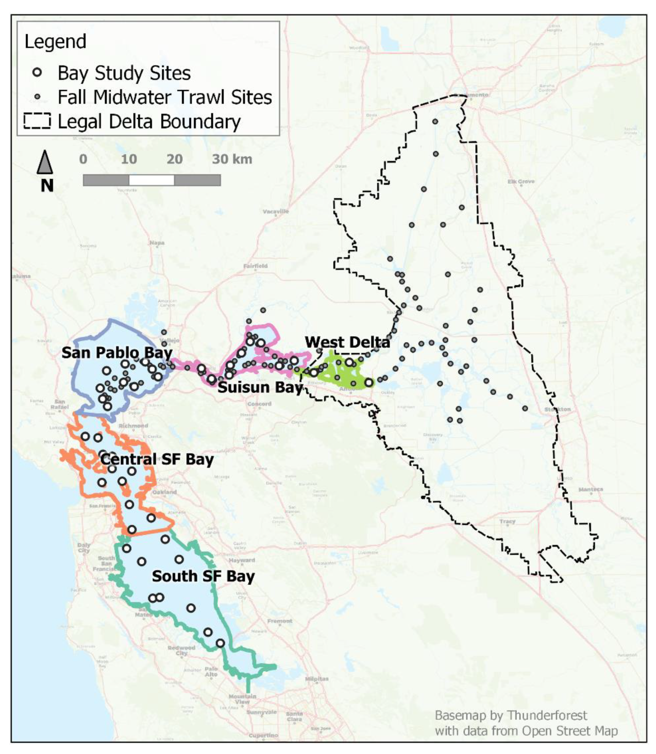
Figure 2.
Smooth functions for the relationship between and the probability of catch a Longfin Smelt in San Pablo Bay and (left column) month of life and (right column) year class identified by birth year, shared across gear types, with various values of k.
Figure 2.
Smooth functions for the relationship between and the probability of catch a Longfin Smelt in San Pablo Bay and (left column) month of life and (right column) year class identified by birth year, shared across gear types, with various values of k.
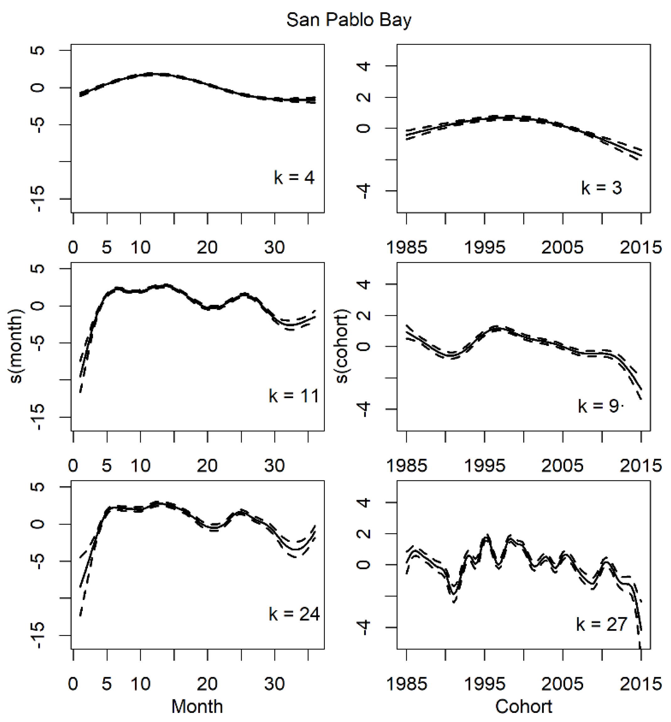
Figure 3.
Mean predicted probability of presence for each region by gear type and by month through the Longfin Smelt life cycle. These are functional means for each region, after registration of individual functions for each cohort.
Figure 3.
Mean predicted probability of presence for each region by gear type and by month through the Longfin Smelt life cycle. These are functional means for each region, after registration of individual functions for each cohort.
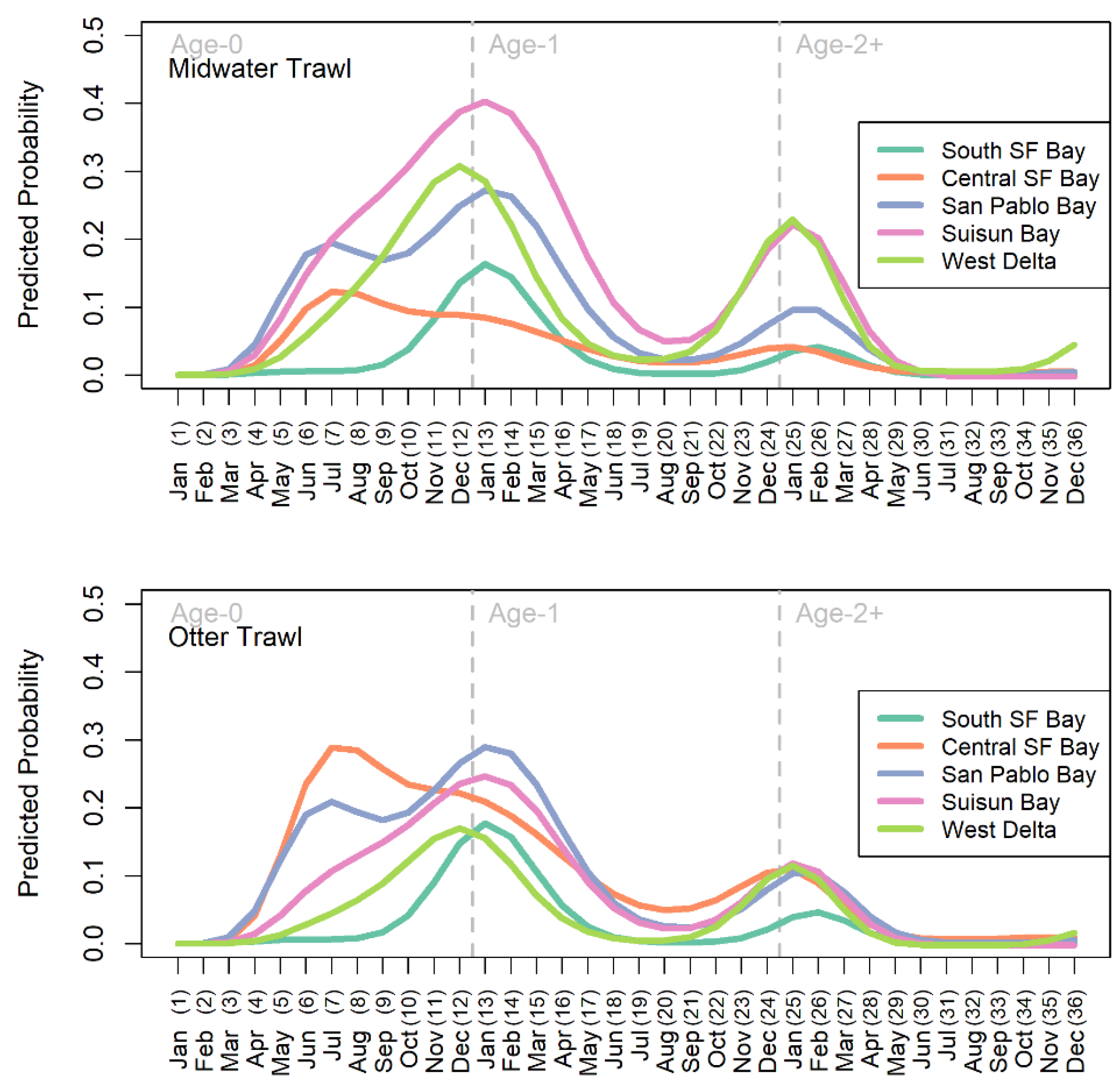
Figure 4.
The Fall Midwater Trawl total annual abundance index and constituent monthly indices for Longfin Smelt over time.
Figure 4.
The Fall Midwater Trawl total annual abundance index and constituent monthly indices for Longfin Smelt over time.
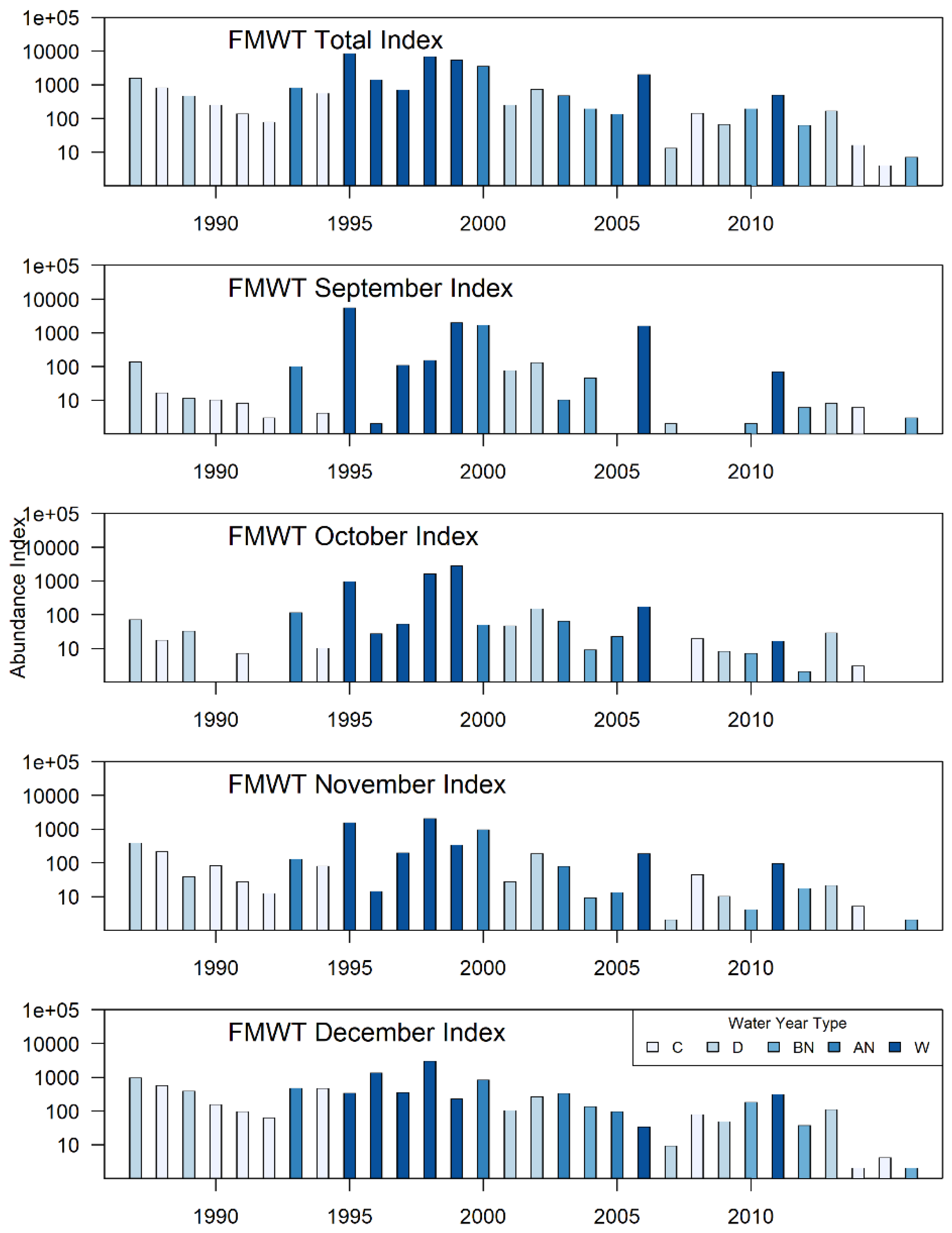
Figure 5.
Month-wise variance in predicted probability associated with a phase shift, rather than a shift in amplitude. These variance estimates come from the variance in the values of the warping functions at each month (for each point, n = 28 year classes).
Figure 5.
Month-wise variance in predicted probability associated with a phase shift, rather than a shift in amplitude. These variance estimates come from the variance in the values of the warping functions at each month (for each point, n = 28 year classes).
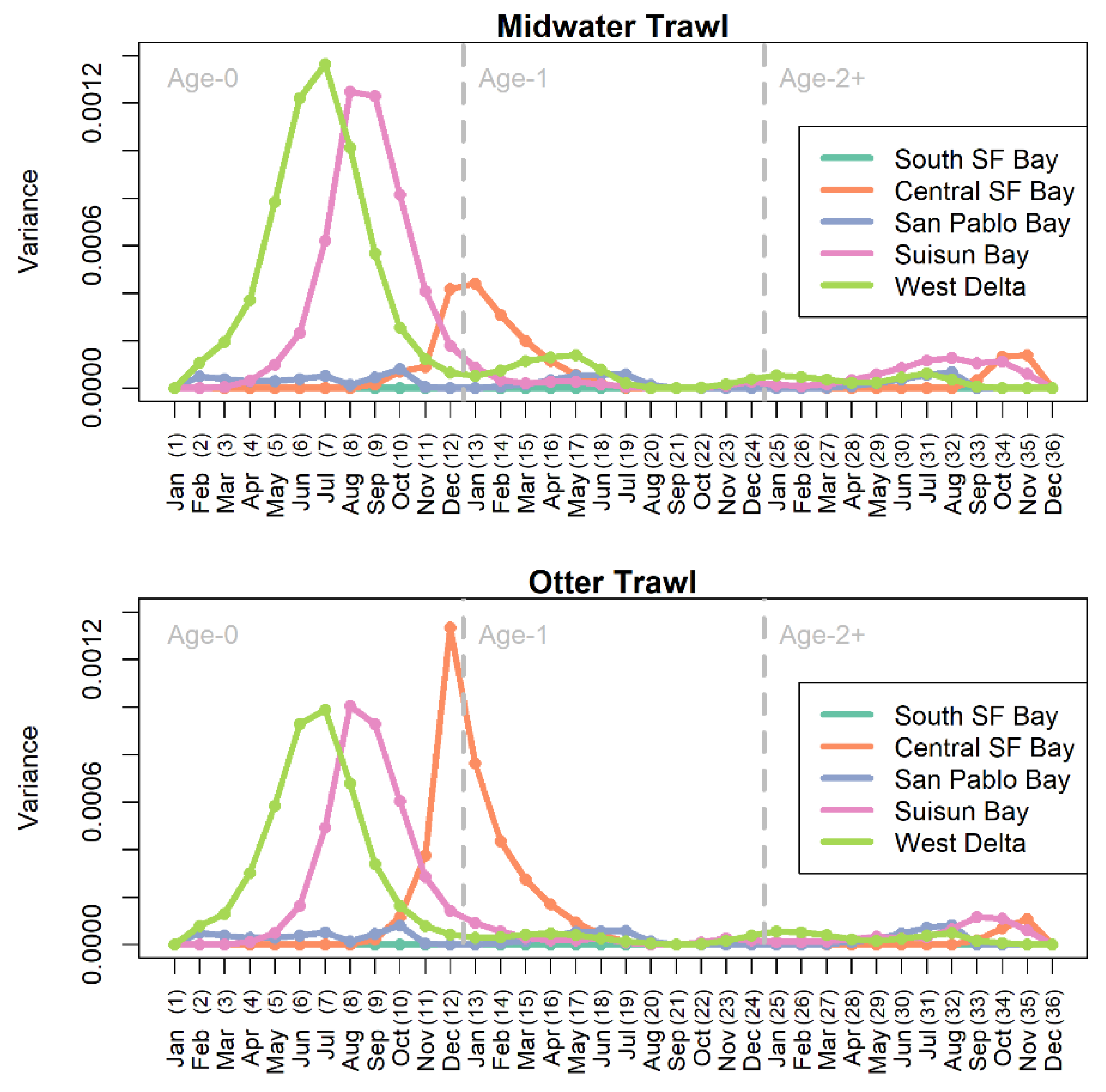
Figure 6.
Shifts in timing of Longfin Smelt presence. Lines represent trends for whichever month had the highest phase variability for each of the regions with spikes in phase variation. South SF Bay and San Pablo Bay did not have spikes in phase variation so those were not included. The horizontal dashed black line at 0 indicates the mean timing of Longfin Smelt presence for each region.
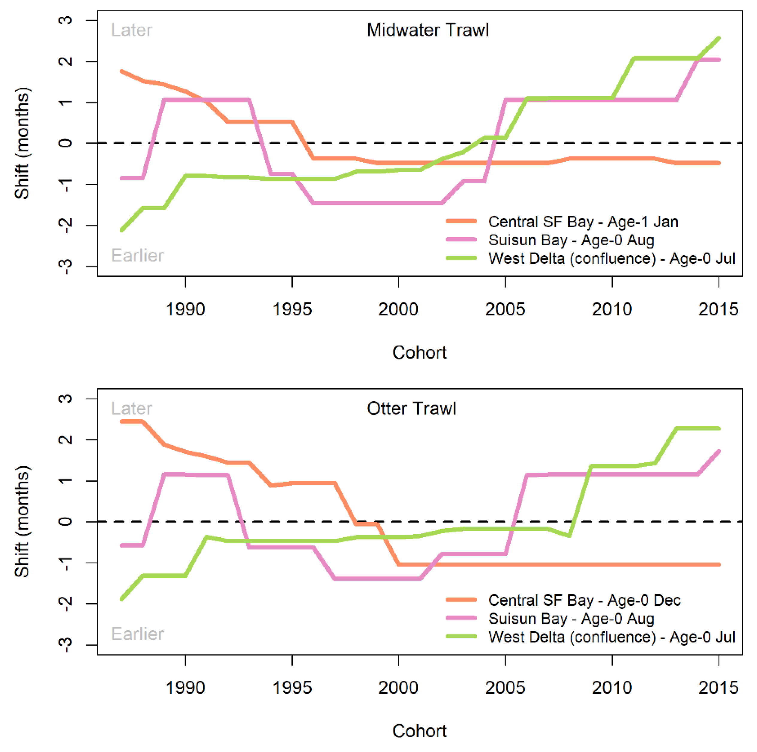

Table 1.
Estimates for parametric coefficients and smooth terms for the selected model. The baseline conditions for parametric coefficients (i.e., where the categorical variables are equal to zero) are bay1 and midwater trawl. Parametric estimates and standard errors are presented in logit-scale. Bay/Region numbering is as follows: 1 = South SF Bay, 2 = Central SF Bay, 3 = San Pablo Bay, 4 = Suisun Bay, 5 = West Delta.
| Parametric coefficients: | ||||||||
| Term | Estimate | Std. error | z value | Pr(>|z|) | ||||
| (Intercept) | -5.18 | 0.18 | -28.37 | < 2e-16 | ||||
| gear:otter trawl | 0.10 | 0.10 | 1.04 | 0.30 | ||||
| bay2 | 0.76 | 0.21 | 3.60 | 0.00 | ||||
| bay3 | 1.66 | 0.20 | 8.20 | 0.00 | ||||
| bay4 | 2.26 | 0.21 | 10.91 | < 2e-16 | ||||
| bay5 | 1.25 | 0.30 | 4.14 | 0.00 | ||||
| otter trawl:bay2 | 1.01 | 0.12 | 8.68 | < 2e-16 | ||||
| otter trawl:bay3 | -0.01 | 0.11 | -0.09 | 0.92 | ||||
| otter trawl:bay4 | -0.90 | 0.11 | -7.95 | 0.00 | ||||
| otter trawl:bay5 | -0.90 | 0.15 | -5.90 | 0.00 | ||||
| Approximate significance of smooth terms: | ||||||||
| Term | edf | Ref.df | Chi.sq | p-value | k’ | edf | k-index | p-value |
| s(month):bay1 | 9.28 | 9.83 | 579.57 | < 2e-16 | 10 | 9.28 | 0.97 | 0.57 |
| s(month36):bay2 | 9.74 | 9.97 | 872.40 | < 2e-16 | 10 | 9.73 | 0.97 | 0.49 |
| s(month):bay3 | 9.80 | 9.99 | 1030.57 | < 2e-16 | 10 | 9.80 | 0.97 | 0.52 |
| s(month):bay4 | 9.71 | 9.97 | 1086.78 | < 2e-16 | 10 | 9.71 | 0.97 | 0.50 |
| s(month):bay5 | 9.29 | 9.82 | 269.28 | < 2e-16 | 10 | 9.29 | 0.97 | 0.45 |
| s(cohort):bay1 | 5.20 | 6.22 | 51.64 | 0.00 | 8 | 5.20 | 0.98 | 0.74 |
| s(cohort):bay2 | 7.56 | 7.93 | 202.43 | < 2e-16 | 8 | 7.56 | 0.98 | 0.74 |
| s(cohort):bay3 | 7.71 | 7.97 | 325.31 | < 2e-16 | 8 | 7.71 | 0.98 | 0.74 |
| s(cohort):bay4 | 7.70 | 7.97 | 393.79 | < 2e-16 | 8 | 7.70 | 0.98 | 0.70 |
| s(cohort):bay5 | 5.88 | 6.87 | 76.39 | 0.00 | 8 | 5.88 | 0.98 | 0.75 |
| ti(month,cohort):bay1 | 1.96 | 2.44 | 1.42 | 0.61 | 16 | 1.96 | 0.94 | 0.01 |
| ti(month,cohort):bay2 | 6.47 | 8.65 | 38.30 | 0.00 | 16 | 6.47 | 0.94 | 0.03 |
| ti(month,cohort):bay3 | 7.73 | 10.10 | 33.24 | 0.00 | 16 | 7.73 | 0.94 | 0.02 |
| ti(month,cohort):bay4 | 10.55 | 12.67 | 42.48 | 0.00 | 16 | 10.55 | 0.94 | 0.03 |
| ti(month,cohort):bay5 | 8.14 | 10.31 | 20.05 | 0.06 | 16 | 8.14 | 0.93 | <2e-16 |
Table 2.
Variance in functions representing predicted probabilities for each bay/region and gear type. Each variance value was derived from the registration of 28 predicted probability curves. Values given with 3 significant figures. Variance in amplitude is relative to the probability of observing Longfin Smelt; units for phase variance are months.
| Region number | Region name | Midwater trawl | Otter trawl | ||
|---|---|---|---|---|---|
| Amplitude | Phase | Amplitude | Phase | ||
| 1 | South SF Bay | 0.0141 | 0.00 | 0.0163 | 0.00 |
| 2 | Central SF Bay | 0.0264 | 0.000184 | 0.108 | 0.00167 |
| 3 | San Pablo Bay | 0.18 | 0.000986 | 0.198 | 0.00113 |
| 4 | Suisun Bay | 0.296 | 0.0106 | 0.163 | 0.00321 |
| 5 | West Delta | 0.113 | 0.0129 | 0.0517 | 0.00262 |
Disclaimer/Publisher’s Note: The statements, opinions and data contained in all publications are solely those of the individual author(s) and contributor(s) and not of MDPI and/or the editor(s). MDPI and/or the editor(s) disclaim responsibility for any injury to people or property resulting from any ideas, methods, instructions or products referred to in the content. |
© 2023 by the authors. Licensee MDPI, Basel, Switzerland. This article is an open access article distributed under the terms and conditions of the Creative Commons Attribution (CC BY) license (http://creativecommons.org/licenses/by/4.0/).
Copyright: This open access article is published under a Creative Commons CC BY 4.0 license, which permit the free download, distribution, and reuse, provided that the author and preprint are cited in any reuse.


