4.3.1. Description of Manuscript-2-2.R
Here, the
library function is used to call the package "sensitivity" which has been implemented in R and goes as an argument into the function
library. Details of the package can be found in Pujol et al. [
9]. Next we define a function, using the function
function and give this function a name
new.name. The function takes in as argument, a two dimensional matrix
X.
k is the number of genes under consideration out of a set of genes. The
new.name implements the g-function (a model) that is used to assign weights to each of the genes, with a random weight. For this,
runif function is used.
b is updated as each gene is considered one at a time in the
for loop. At the end of the function, value in
b is returned implicity. What happens is as the loop iterates
length(
a) times, were the expression shows the number of genes the user has selected. Note that lenght if
a is computed using the value of
k. This function read within lines 3-10. Also,
genSampleComb is a function which returns a two dimensional matrix with the a specific number of columns defined in
yCol. More about this function will be talked at a later stage. Here, definitions of the functions are provided (see lines 1-14).
1 library(sensitivity)
2 # Function definitions
3 new.fun <- function(X){
4 a <- runif(k)
5 b <- 1
6 for (j in 1:length(a)) {
7 b <- b * (abs(4 * X[, j] - 2) +
a[j])/(1 + a[j])
8 }
9 b
10 }
11
12 genSampleComb <- function(yCol){
13 return(disty[,yCol])
14 }
15
Since the code can be adapted for different data sets, a query is asked to the user regarding the generation of distribution around point measurements, if they exist in the data under consideration. To query the user, the function readline is employed. The user has to type in the option provided in the query for a particular functionality to take affect. Here, the response to the query is stored in the variable DISTRIBUTION. Next, if the response in DISTRIBUTION is a yes, that is, the user typed in "y", then the ensuing block within the if command will get executed, else it will be skipped. Again, the block under consideration, defines a new function gdfetppv which takes in arguments n and yt, were n contains the number of points which a user might want to generate for a distribution around a numerical point estimate. The measured numerical point estimates for each gene under consideration are assorted in a vector yt. The length of yt shows the number of genes involved in the study of sensitivity analysis. As the for iterates through each gene, for the corresponding numerical point estimate for a partipular gene, a distribution around the point estimate is generated with the mean value being yt[i] (i is the iterator) and a standard deviation of . Along with the distribution a minor jitter or noise is added. Thus, the whole distribution is stored in a vector. Note that the output of the jitter function is a vector and R stores vector in column format. Consequently, as the for loop iterates from one gene to another, the columns are bound together using a column binding function cbind. Thus, randyt keeps on increasing column wise, till all genes have been covered. Once out of the loop, the row vector yt is appended with the distribution matrix randyt using row binding function rbind. The output of the function is a two dimensional matrix containing the point estimate in the first row and the corresponding distribution in the rows below (see lines 20-28).
16 # Generation of distributions
17 DISTRIBUTION <- readline("Should i generate
distribution of data [y/n] - ")
19 if(DISTRIBUTION == "y"){
20 gdfetppv <- function(n,yt){
21 randyt <- c()
22 lenyt <- length(yt)
23 for(i in 1:lenyt){
24 randyt <- cbind(randyt,
jitter(rnorm(n, mean = yt[i],
sd = 0.005), factor = 1))
25 }
26 yt <- rbind(yt, randyt)
27 return(yt)
28 }
29 }
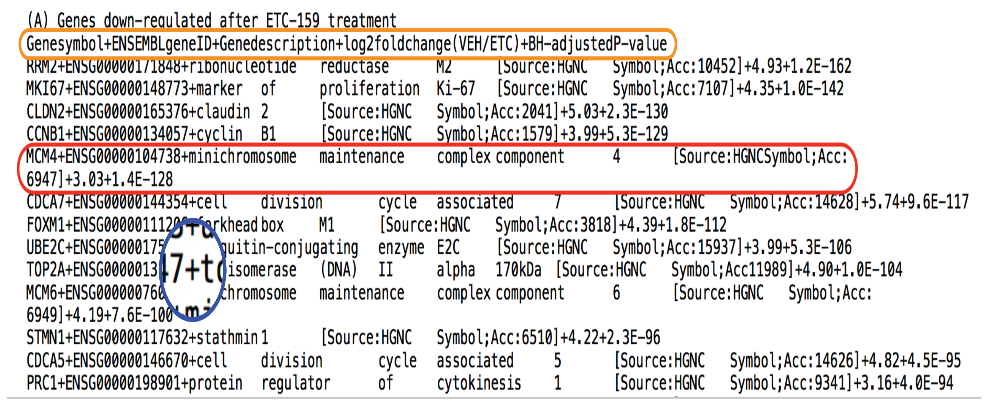
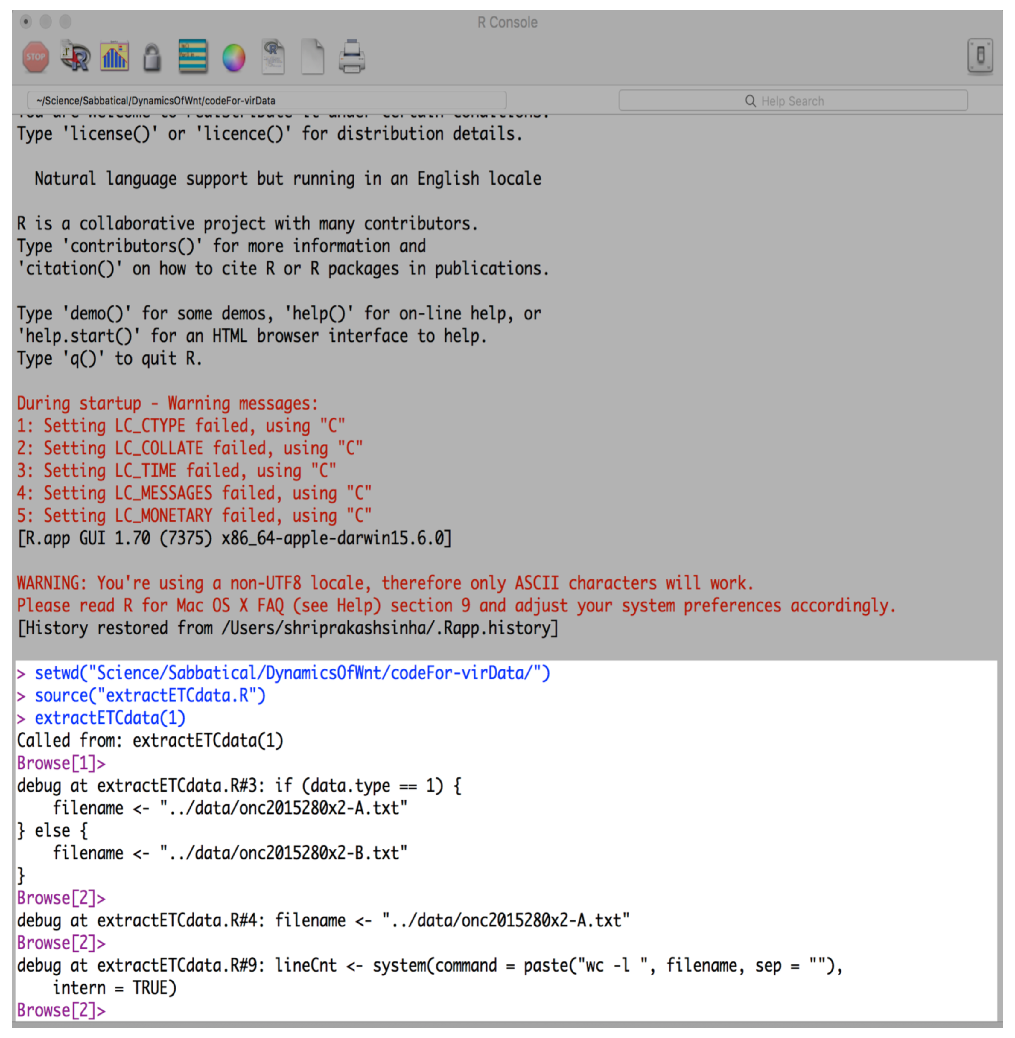
After the functions have been defined, the main execution begins. The code starts with the extraction fo the data using the readline argument and provides an option to the used to choose file that contains data regarding down regulated genes or up regulated genes. Once the respone is recorded, it is stored in the variable DATATYPE. If the user enters a wrong number, then a while loop is run which asks to enter the right response. This feedback continues till the user enters the right response (see lines 30-33). After the correct response is recorded, we use the function extractETCdata to extract the information from the particular file associated with the response in DATATYPE. This is done using the command extractETCdata(DATATYPE) and the output of the function is stored in oncETCmain. We keep a copy of the stored information in oncETCmain and make a second copy in the subsequent line in oncETC(see line 34-35). This manuscript explains the code for retrieving 2nd order combination, only so as to set a platform for many who would be reading the article. Note, before the use of the function i.e. instantiation of the function, the function needs to be defined and initialized. We defined the function and named it. After that an instance of the function is used to get a certain result. One instance is extractETCdata(1) and another instance is extractETCdata(2).
30 # Data extraction
31 DATATYPE <- readline("Choose a file to
process [1/2] \n
1 - ../data/onc2015280x2-A.txt \n
Genes down-regulated after ETC-159
treatment \n
2 - ../data/onc2015280x2-B.txt \n
Genes up-regulated after ETC-159
treatment \n
File number - ")
32 while(DATATYPE != "1" & DATATYPE != "2"){
DATATYPE <- readline("Type the kind of
data to be processed [1/2] - ")
33 }
34 oncETCmain <- extractETCdata(DATATYPE)
35 oncETC <- oncETCmain
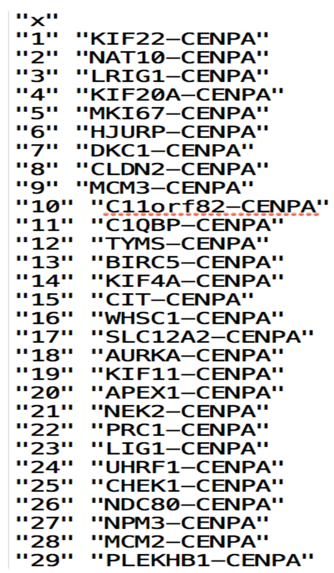
Of interest is the column containing the fold change numerical point estimates that are stored in the variable oncETC. Since the information under this column is stored in the data frame, it needs to be converted into a matrix for further processing by sensitivity analysis package. For this, as.matrix function is used which takes in the object in x along with arguments ncol which asks for the number of columns into which the information needs to be divided and byrow being false stating that the information will not be lined up row wise, but column wise. The result of the transformation is stored in y. Next, respective column elements in y are allotted their gene names. This is acheived using oncETC$Genesymbol. The rownames of y which depict the gene names are thus assigned. We also save the names of the genes in factor.names variable. The dimension or the size of y in terms of number of rows and number of columns is recorded using the function dim and the measurements are stored in dim.y. dim.y[1] contains the number of rows which implicitly defines the number of genes (stored in no.genes). The whole list of genes can be shown on the command prompt during the execution of the code via cat(rownames(y)) (see lines 35-40).
35 y <- as.matrix(x = oncETC$logTwoFC,
ncol = 1, byrow = FALSE)
36 rownames(y) <- oncETC$Genesymbol
37 factor.names <- oncETC$Genesymbol
38 dim.y <- dim(y)
39 no.genes <- dim.y[1]
40 cat(rownames(y))
Next, the user is asked which gene the user would like to investigate and the response is stored in geneName. Also, since the pipeline is about investigating combinations, we need to input the number of combinations we are interested in. For this, a similar query is asked and the value is stored in the variable k. Since it is in the character format, it needs to be converted into a numerical format and that is done using as.numeric function. The cat function helps in displaying messages to ease the user to understand what is happening while execution of the program. The combinations that can be generated from k genes, out of the total number of genes no.genes is computed using combn. This returns a two dimensional matrix to geneComb whose number of columns represent the total number of combinations, i.e dim(geneComb[2]) (see lines 41-47).
41 geneName <- readline("\nEnter name of
gene to be evaluated - ")
42 # Regarding combinations
43 ANSWER <- readline("nCk - choosing k - ")
44 k = as.numeric(ANSWER)
45 cat("choosing ",k," out of the",
no.genes," genes!\n---\n")
46 geneComb <- combn(no.genes,k)
47 no.geneComb <- dim(geneComb)[2]
Next, initialization of the variables needs to be done for processing of the data. A series of list data structure is initialized and names are assigned to each new list as shown from lines 49 to 60. These are the variables where the sensitivity indicies will be stored. siNames contains the names of the indicies which the search engine uses and the user can pick any one of them for computation. Line 63 prompts the user to enter the name of the sensitivity index, after looking at displayed list in the command on line 62. This name is stored in the variable varName. Next, we search for the pattern (stored in varName) in some of the Sobol index names and if the user has chosen a sobol sensitivity index, then ISSOBOL is assigned to a true value. This will be used and explained later on (see lines 49-66).
48 # some initializations
49 sensiFdiv.TV <- list()
50 sensiFdiv.KL <- list()
51 sensiFdiv.Chi2 <- list()
52 sensiFdiv.Hellinger <- list()
53 sensiHSIC.rbf <- list()
54 sensiHSIC.linear <- list()
55 sensiHSIC.laplace <- list()
56 SB.jansen <- list()
57 SB.2002 <- list()
58 SB.2007 <- list()
59 SB.martinez <- list()
60 SBL <- list()
61 siNames <- c("Fdiv.TV", "Fdiv.KL",
"Fdiv.Chi2", "Fdiv.Hellinger", "HSIC.rbf",
"HSIC.linear", "HSIC.laplace", "SB.2002",
"SB.2007", "SB.jansen", "SB.martinez", "SBL")
62 cat("Types of SA - ", siNames, "\n")
63 varName <- readline("Enter a type of SA - ")
64 ISSOBOL <- FALSE
65 if(length(grep(varName, "SB.2002"))!= 0 |
length(grep(varName, "SB.2007"))!= 0 |
length(grep(varName, "SB.jansen"))!= 0 |
length(grep(varName, "SB.martinez"))!= 0
| length(grep(varName, "SBL"))!= 0){
ISSOBOL <- TRUE
66 }
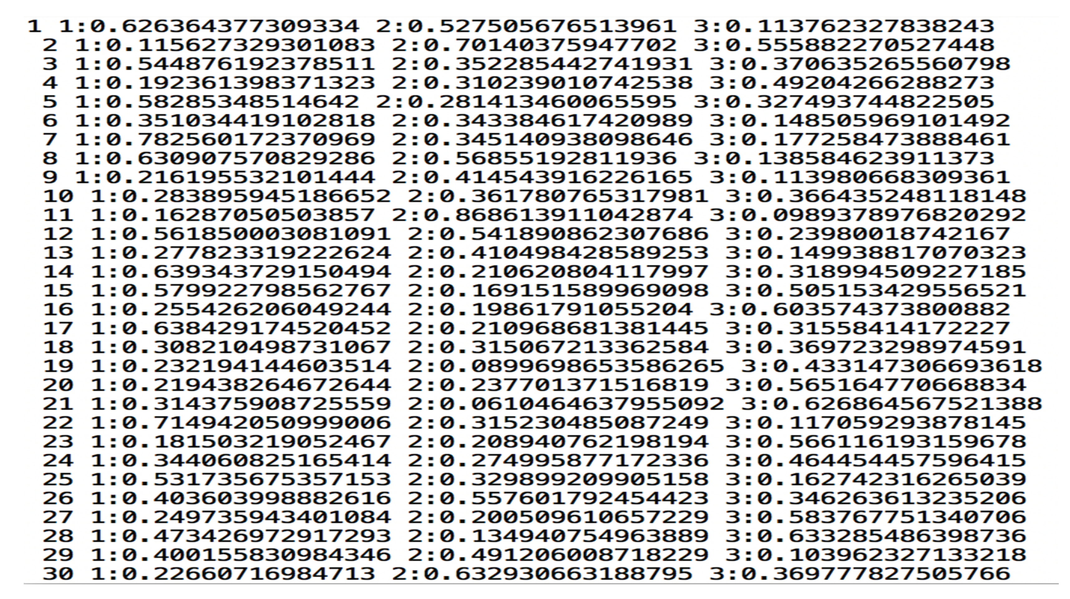
Regarding the generation of distribution of numerical point measurements, it is important to specify the number of samples. The user is usually given a choice as shown in line 67 (here commented). However, for exercise purpose, we set the value of number of samples to be . Next, the function for generating distribution of size 9 per gene measurement is used and the output is converted into a data frame using the function data.frame. This data frame is then stored in variable disty or distribution of y. We again save the number of samples as an extra using the dim function, in a variable no.Samples (see lines 67-71).
67 # n <- as.numeric(readline("Enter number of
samples for distribution (odd numeric) - "))
68 n <- 9
69 disty <- data.frame(gdfetppv(n,t(y)))
70 no.Samples <- dim(disty)[1]
71 cat("generating sample combinations!\n")
The apply function is one of the important functions in R langauge and widely used for vector programming. It is important here in the sense that we need to compute the indices for combinations of factors. The arguments for apply take in a matrix, the indicator for a vector in a matrix over which a function will be applied. Here we see that geneComb is the matrix containing the combinations of genes; MARGIN with an indicator 2 means the columns of geneComb will be worked upon by the function genSampleComb in the variable FUN. Thus the function apply will apply the function genSampleComb to the columns of the matrix geneComb. The function genSampleComb in line 12, takes in a column of the matrix geneComb and returns the k distributions that are stored in the matrix disty. So, if k is 2, then the number of rows in geneComb will be 2. These 2 elements associated with a particular column in geneComb will contain the gene numbers in a list of genes. During the application of the apply function, yCol stores a column of geneComb and uses genSampleComb to generate disty[,yCol], a matrix, were n is number of samples and k is the number of elements in combination. The procedure is applied to all columns of geneComb, for this. (see line 72).
72 distyN <- apply(X = geneComb, MARGIN = 2,
FUN = genSampleComb)
Next, the combinatorial distributions stored in distyN are processed to segregate the gene combinations that contain the particular gene of interest defined by the user from a list of gene, in geneName. List variables are defined and to find combinations containing geneName, a for loop is executed were the iterator iterates through the total number of combinations. For each of the combination contained in names(distyN[i]), if geneName is found to be existing, then the distribution containing geneName and another gene in distyN[i] is stored in x.S, a list. For every such identification, a counter cnt is incremented. Finally, after all combinations have been found which contain geneName, the final is assigned to number of selected gene combinations no.slgeneComb (see lines 73-85).
73 # Sample with replicates
74 x.S <- list()
75 x.Sfh <- list()
76 x.Ssh <- list()
78 cnt <- 0
79 for(i in 1:no.geneComb){
80 if(geneName %in% names(distyN[[i]])){
81 cnt <- cnt + 1
82 x.S[[cnt]] <- distyN[[i]]
83 }
84 }
85 no.slgeneComb <- cnt
Usually a user will be asked about the total number of iterations for which the sensitivity indicies will be generated. This is done to get an average sensitivity index score which is then used for ranking of the combinations. For demonstration purpose, we set the iteration number to itrNo . The for loops the iterator for 50 iterations. Every iteration, the number of interation is displayed at the start of the for loop. The samples need to be shuffled every time in order to have variation so that the mean of the sensitivity indices can be generated. This can be done by using the function sample which take a range of values from 1 to no.Samples and the size of the sample is set to no.Samples. The shuffled samples are stored in sample.index. idx.fh and idx.sh are used to divide the sample into two halves, in case one is using Sobol method for generating sensitivity indicies. Next, if the method used is Sobol or a variant of the same, as indicated by , then shuffling of the samples in combination happens. This shuffling is done in lines 99-100, for all combinations, i.e j from 1 to no.slgeneComb. For, non Sobol based methods, the shuffling is simple as shown in line 104.
86 # itrNo <- as.numeric(readline("Number
of iterations for averaged ranking - "))
87 itrNo <- 50
88 hmean <- list()
89 for(itr in 1:itrNo){
90 # disty <- data.frame(gdfetppv(n,yt))
91 # distyN can be replaced with x.S also
92 cat("generating for sample - ", itr, "\n")
93 sample.index <- sample(x = 1:no.Samples,
size = no.Samples)
94 idx.fh <- sample.index[1:(no.Samples/2)]
95 idx.sh <- sample.index[((no.Samples/2)+1)
:no.Samples]
96 # Shuffle the samples
97 if(ISSOBOL){
98 for(j in 1:no.slgeneComb){
99 x.Sfh[[j]] <- x.S[[j]][idx.fh,]
100 x.Ssh[[j]] <- x.S[[j]][idx.sh,]
101 }
102 }else{
103 for(j in 1:no.slgeneComb){
104 x.S[[j]] <- x.S[[j]][sample.index,]
105 }
106 }
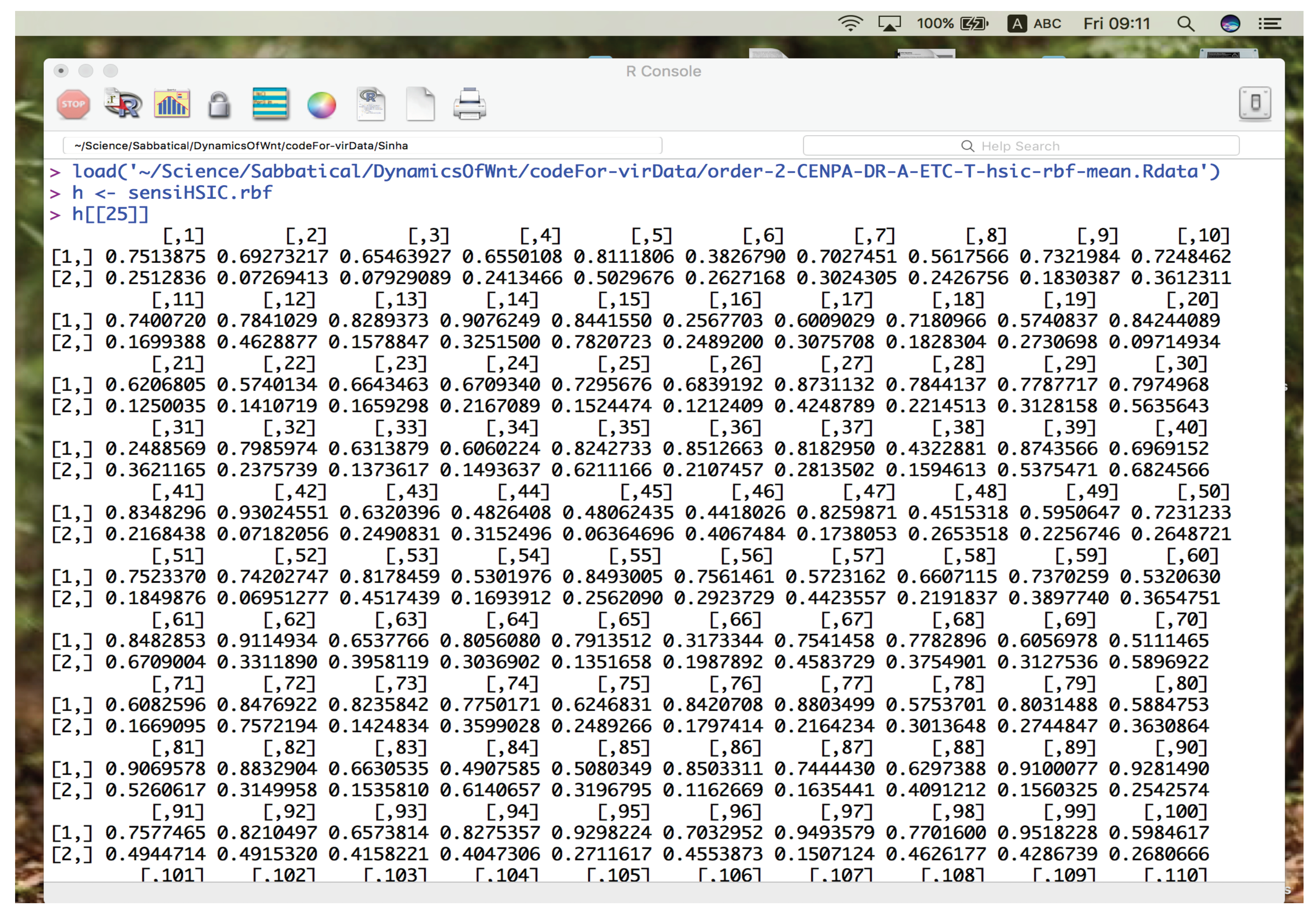
Once the samples for the combinations have been stored in
x.S, it is time to generate the sensitivity indicies. To generate a sensitivity index of a particular type, the user has to specify the name of the sensitivity index. This has already been done earlier and the name is stored in
varName. What follows is a series of condition tests using the
if ... else to know which type of sensitivity method needs to be taken into account and necessary method to be initiated to generate the indicies. One of the approach would be to use
grep function which searches for a pattern in
varName. If the pattern exists, then the length of the finding would not be zero. When this condition holds, then a particular index associated with the pattern is intiated. So, if "TV" is the pattern and it found to be in the
varName, then f-divergence method Csiszár et al. [
10] with a Total variation distance
needs to be initiated. The short explanation on the theoretical principles of density and variance based methods has been explained in Sinha [
2]. Here we concentrate on the flow of the code. In line 109, we define and initialize a new variable
FdivTV. After some displays on the screen,
lapply is used on
x.S.
lapply returns a list of the same length as
x.S, each element of which is the result of applying function
sensiFdiv to the corresponding element of
x.S. Additionally, since the sensitivity method uses a model function, we use extra arguments in the
lapply function, like
model =
new.fun;
nboot = 0 and
conf = 0.95. This
new.fun has earlier been defined in the beginning of the code. So,
lapply generates sensitivity indices for each of the matricies containing a specific gene combination using the
new.fun via
sensiFdiv. The result is stored in a variable
h. Since we know that
lapply will generate sensitivity indices for each of the matrices in
x.S, thus each combination has an associated sensitivity that is stored in
h[[p]]$S$original. We bind this to the variable
FdivTV (see lines 108-113).
Next, since the for loop in line 89 works for many iterations, we need to store the sensitivity index computed in this iteration in a certain variable. This is done in sensiFdiv.TV[[itr]], definition of which was done in line 49. Also, if this is the first iteration, then we define the file name based on the data that is being used and the iteration (see lines 115-117).
107 # itr <- 1
108 if(length(grep("TV",varName))!= 0){
109 FdivTV <- c()
110 cat("computing estimate different
indices ...\n")
111 cat("Fdiv SA - TV\n")
112 h <- lapply(x.S, sensiFdiv,
model = new.fun, fdiv = "TV",
nboot = 0, conf = 0.95)
113 for(p in 1:no.slgeneComb){
FdivTV <- cbind(FdivTV,
h[[p]]$S$original)
}
114 sensiFdiv.TV[[itr]] <- FdivTV
115 if(DATATYPE == "1" & itr == 1){
filename <- paste("order-",k,"-",
geneName,
"-DR-A-ETC-T-fdiv-tv-mean.Rdata",
sep = "")
116 }else if(DATATYPE == "2" & itr == 1){
filename <- paste("order-",k,"-",
geneName,
"-UR-A-ETC-T-fdiv-tv-mean.Rdata",
sep = "")
117 }
The next series of conditions deals with the different methods in a similar manner as explained for lines 108-117. Lines 118-130 talk about f-divergence method Csiszár et al. [
10] with a Kullback-Leibler divergence
.
118 }else if(length(grep("KL",varName))
!= 0){
119 FdivKL <- c()
120 cat("computing estimate different
indices ...\n")
121 cat("Fdiv SA - KL\n")
122 h <- lapply(x.S, sensiFdiv,
model = new.fun, fdiv = "KL",
nboot = 0, conf = 0.95)
123 for(p in 1:no.slgeneComb){
124 FdivKL <- cbind(FdivKL,
h[[p]]$S$original)
125 }
125 sensiFdiv.KL[[itr]] <- FdivKL
126 if(DATATYPE == "1" & itr == 1){
127 filename <- paste("order-",k,"-",
geneName,
"-DR-A-ETC-T-fdiv-kl-mean.Rdata",
sep = "")
128 }else if(DATATYPE == "2" & itr == 1){
129 filename <- paste("order-",k,"-",
geneName,
"-UR-A-ETC-T-fdiv-kl-mean.Rdata",
sep = "")
130 }
Lines 131-144 talk about f-divergence method Csiszár et al. [
10] with a
distance
.
131 }else if(length(grep("Chi2",varName))
!= 0){
132 FdivChi2 <- c()
133 cat("computing estimate different
indices ...\n")
134 cat("Fdiv SA - Chi2\n")
135 h <- lapply(x.S, sensiFdiv,
model = new.fun, fdiv = "Chi2",
nboot = 0, conf = 0.95)
136 for(p in 1:no.slgeneComb){
137 FdivChi2 <- cbind(FdivChi2,
h[[p]]$S$original)
138 }
139 sensiFdiv.Chi2[[itr]] <- FdivChi2
140 if(DATATYPE == "1" & itr == 1){
141 filename <- paste("order-",k,"-",
geneName,
"-DR-A-ETC-T-fdiv-chi2-mean.Rdata",
sep = "")
142 }else if(DATATYPE == "2" & itr == 1){
143 filename <- paste("order-",k,"-",
geneName,
"-UR-A-ETC-T-fdiv-chi2-mean.Rdata",
sep = "")
144 }
Lines 145-158 talk about f-divergence method Csiszár et al. [
10] with a Hellinger distance
.
145 }else if(length(grep("Hellinger",varName))
!= 0){
146 FdivHellinger <- c()
147 cat("computing estimate different
indices ...\n")
148 cat("Fdiv SA - Hellinger\n")
149 h <- lapply(x.S, sensiFdiv,
model = new.fun, fdiv = "Hellinger",
nboot = 0, conf = 0.95)
150 for(p in 1:no.slgeneComb){
151 FdivHellinger <- cbind(FdivHellinger,
h[[p]]$S$original)
152 }
153 sensiFdiv.Hellinger[[itr]]
<- FdivHellinger
154 if(DATATYPE == "1" & itr == 1){
155 filename <- paste("order-",k,"-",
geneName,
"-DR-A-ETC-T-fdiv-hellinger-mean.Rdata",
sep = "")
156 }else if(DATATYPE == "2" & itr == 1){
157 filename <- paste("order-",k,"-",
geneName,
"-UR-A-ETC-T-fdiv-hellinger-mean.Rdata",
sep = "")
158 }
Da Veiga [
11] recently proposed a new set of dependence measures using kernel methods. These also, have been implemented in Pujol et al. [
9]. The following contains variants of different kernels involved in computing the sensitvity indices. Lines 159-172 show similar execution code as above with changes insome of the arguments in the
lapply function. Here, the "rbf" or radial basis function is used within
sensiHSIC.
159 }else if(length(grep("rbf",varName))
!= 0){
160 HSICrbf <- c()
161 cat("computing estimate different
indices ...\n")
162 cat("HSIC SA - rbf kernel\n")
163 h <- lapply(x.S, sensiHSIC,
model = new.fun, kernelX = "rbf",
paramX = NA, kernelY = "rbf",
paramY = NA, conf = 0.95)
164 for(p in 1:no.slgeneComb){
165 HSICrbf <- cbind(HSICrbf,
h[[p]]$S$original)
166 }
167 sensiHSIC.rbf[[itr]] <- HSICrbf
168 if(DATATYPE == "1" & itr == 1){
169 filename <- paste("order-",k,"-",
geneName,
"-DR-A-ETC-T-hsic-rbf-mean.Rdata",
sep = "")
170 }else if(DATATYPE == "2" & itr == 1){
171 filename <- paste("order-",k,"-",
geneName,
"-UR-A-ETC-T-hsic-rbf-mean.Rdata",
sep = "")
172 }
Lines 173-186 show similar execution code as above with changes insome of the arguments in the lapply function. Here, the linear function is used.
173 }else if(length(grep("linear",varName))
!= 0){
174 HSIClinear <- c()
175 cat("computing estimate different
indices ...\n")
176 cat("HSIC SA - linear kernel\n")
177 h <- lapply(x.S, sensiHSIC,
model = new.fun, kernelX = "linear",
paramX = NA, kernelY = "linear",
paramY = NA, conf = 0.95)
178 for(p in 1:no.slgeneComb){
179 HSIClinear <- cbind(HSIClinear,
h[[p]]$S$original)
180 }
181 sensiHSIC.linear[[itr]] <- HSIClinear
182 if(DATATYPE == "1" & itr == 1){
183 filename <- paste("order-",k,"-",
geneName,
"-DR-A-ETC-T-hsic-linear-mean.Rdata",
sep = "")
184 }else if(DATATYPE == "2" & itr == 1){
185 filename <- paste("order-",k,"-",
geneName,
"-UR-A-ETC-T-hsic-linear-mean.Rdata",
sep = "")
186 }
Lines 187-200 show similar execution code as above with changes insome of the arguments in the lapply function. Here, the laplace function is used.
187 }else if(length(grep("laplace",varName))
!= 0){
188 HSIClaplace <- c()
189 cat("computing estimate different
indices ...\n")
190 cat("HSIC SA - laplace kernel\n")
191 h <- lapply(x.S, sensiHSIC,
model = new.fun, kernelX = "laplace",
paramX = NA, kernelY = "laplace",
paramY = NA, conf = 0.95)
192 for(p in 1:no.slgeneComb){
193 HSIClaplace <- cbind(HSIClaplace,
h[[p]]$S$original)
194 }
195 sensiHSIC.laplace[[itr]] <- HSIClaplace
196 if(DATATYPE == "1" & itr == 1){
197 filename <- paste("order-",k,"-",
geneName,
"-DR-A-ETC-T-hsic-laplace-mean.Rdata",
sep = "")
198 }else if(DATATYPE == "2" & itr == 1){
199 filename <- paste("order-",k,"-",
geneName,
"-UR-A-ETC-T-hsic-laplace-mean.Rdata",
sep = "")
200 }
Finally, we come to the section, were variants of the Sobol function have been encoded. It is here that the use of divided samples
X.Sfh and
X.Ssh comes to play. We do not use the
lapply function. Instead, the Sobol’ [
12] variants are enconded using name specific function (see below). Lines 201-214 show similar execution code as above, but using
soboljansen.
201 }else if(length(grep("jansen",varName))
!= 0){
202 SBLjansen <- c()
203 cat("computing estimate different
indices ...\n")
204 cat("Sobol Jansen SA\n")
205 for(p in 1:no.slgeneComb){
206 h <- soboljansen(model = new.fun,
X1 = t(x.Sfh[[p]]),
X2 = t(x.Ssh[[p]]), conf = 0.95)
207 SBLjansen <- cbind(SBLjansen,
c(h$S$original, h$T$original))
208 }
209 SB.jansen[[itr]] <- SBLjansen
210 if(DATATYPE == "1" & itr == 1){
211 filename <- paste("order-",k,"-",
geneName,
"-DR-A-ETC-T-sb-jansen-mean.Rdata",
sep = "")
212 }else if(DATATYPE == "2" & itr == 1){
213 filename <- paste("order-",k,"-",
geneName,
"-UR-A-ETC-T-sb-jansen-mean.Rdata",
sep = "")
214 }
Lines 215-228 show similar execution code as above, but using sobol2002.
215 }else if(length(grep("2002",varName))
!= 0){
216 SBL2002 <- c()
217 cat("computing estimate different
indices ...\n")
218 cat("Sobol 2002 SA\n")
219 for(p in 1:no.slgeneComb){
220 h <- sobol2002(model = new.fun,
X1 = t(x.Sfh[[p]]),
X2 = t(x.Ssh[[p]]), conf = 0.95)
221 SBL2002 <- cbind(SBL2002,
c(h$S$original, h$T$original))
222 }
223 SB.2002[[itr]] <- SBL2002
224 if(DATATYPE == "1" & itr == 1){
225 filename <- paste("order-",k,"-",
geneName,
"-DR-A-ETC-T-sb-2002-mean.Rdata",
sep = "")
226 }else if(DATATYPE == "2" & itr == 1){
227 filename <- paste("order-",k,"-",
geneName,
"-UR-A-ETC-T-sb-2002-mean.Rdata",
sep = "")
228 }
Lines 229-242 show similar execution code as above, but using sobol2007.
229 }else if(length(grep("2007",varName))
!= 0){
230 SBL2007 <- c()
231 cat("computing estimate different
indices ...\n")
232 cat("Sobol 2007 SA\n")
233 for(p in 1:no.slgeneComb){
234 h <- sobol2007(model = new.fun,
X1 = t(x.Sfh[[p]]),
X2 = t(x.Ssh[[p]]), conf = 0.95)
235 SBL2007 <- cbind(SBL2007,
c(h$S$original, h$T$original))
236 }
237 SB.2007[[itr]] <- SBL2007
238 if(DATATYPE == "1" & itr == 1){
239 filename <- paste("order-",k,"-",
geneName,
"-DR-A-ETC-T-sb-2007-mean.Rdata",
sep = "")
240 }else if(DATATYPE == "2" & itr == 1){
241 filename <- paste("order-",k,"-",
geneName,
"-UR-A-ETC-T-sb-2007-mean.Rdata",
sep = "")
242 }
Lines 243-256 show similar execution code as above, but using sobolmartinez.
243 }else if(length(grep("martinez",varName))
!= 0){
244 SBLmartinez <- c()
245 cat("computing estimate different
indices ...\n")
246 cat("Sobol Martinez SA\n")
247 for(p in 1:no.slgeneComb){
248 h <- sobolmartinez(model = new.fun,
X1 = t(x.Sfh[[p]]),
X2 = t(x.Ssh[[p]]), conf = 0.95)
249 SBLmartinez <- cbind(SBLmartinez,
c(h$S$original, h$T$original))
250 }
251 SB.martinez[[itr]] <- SBLmartinez
252 if(DATATYPE == "1" & itr == 1){
253 filename <- paste("order-",k,"-",
geneName,
"-DR-A-ETC-T-sb-martinez-mean.Rdata",
sep = "")
254 }else if(DATATYPE == "1" & itr == 1){
255 filename <- paste("order-",k,"-",
geneName,
"-UR-A-ETC-T-sb-martinez-mean.Rdata",
sep = "")
256 }
Lines 257-272 show similar execution code as above, but using sobol.
257 }else if(length(grep("SBL",varName))
!= 0){
258 sbl <- c()
259 cat("computing estimate different
indices ...\n")
260 cat("SBL SA\n")
261 for(p in 1:no.slgeneComb){
262 h <- sobol(model = new.fun,
X1 = t(x.Sfh[[p]]),
X2 = t(x.Ssh[[p]]), order = 1,
conf = 0.95)
263 sbl <- cbind(SBL, c(h$S$original,
h$T$original))
264 }
265 SBL[[itr]] <- sbl
266 if(DATATYPE == "1" & itr == 1){
267 filename <- paste("order-",k,"-",
geneName,
"-DR-A-ETC-T-sbl-mean.Rdata",
sep = "")
268 }else if(DATATYPE == "2" & itr == 1){
269 filename <- paste("order-",k,"-",
geneName,
"-UR-A-ETC-T-sbl-mean.Rdata",
sep = "")
270 }
271 }
272 }
Once the indices have been generated, they need to be stored in a file for further processing. The following set of lines help in saving the work, were the function save is used and variables no.slgeneComb, x.S and the respective sensitivity indices related to varName is stored in the filename.
273 if(length(grep("TV",varName))!= 0){
274 save(no.slgeneComb, x.S,
sensiFdiv.TV, file = filename)
275 }else if(length(grep("KL",varName))
!= 0){
276 save(no.slgeneComb, x.S,
sensiFdiv.KL, file = filename)
277 }else if(length(grep("Chi2",varName))
!= 0){
276 save(no.slgeneComb, x.S,
sensiFdiv.Chi2, file = filename)
277 }else if(length(grep("Hellinger",varName))
!= 0){
278 save(no.slgeneComb, x.S,
sensiFdiv.Hellinger, file = filename)
279 }else if(length(grep("rbf",varName))
!= 0){
280 save(no.slgeneComb, x.S,
sensiHSIC.rbf, file = filename)
281 }else if(length(grep("linear",varName))
!= 0){
282 save(no.slgeneComb, x.S,
sensiHSIC.linear, file = filename)
283 }else if(length(grep("laplace",varName))
!= 0){
284 save(no.slgeneComb, x.S,
sensiHSIC.laplace, file = filename)
285 }else if(length(grep("jansen",varName))
!= 0){
286 save(no.slgeneComb, x.S,
SB.jansen, file = filename)
287 }else if(length(grep("2002",varName))
!= 0){
289 save(no.slgeneComb, x.S,
SB.2002, file = filename)
290 }else if(length(grep("2007",varName))
!= 0){
291 save(no.slgeneComb, x.S,
SB.2007, file = filename)
292 }else if(length(grep("martinez",varName))
!= 0){
293 save(no.slgeneComb, x.S,
SB.martinez, file = filename)
294 }else if(length(grep("SBL",varName))
!= 0){
295 save(no.slgeneComb, x.S,
SBL, file = filename)
296 }
This ends the coding part of estimating sensitvity indices. Once the indices are ready they can be used in various ways for evaluation of the combinations. Here, we use one of the ways to ranking these scores. However, not that there is no one definite rule to say that one has to rank in this way only. It depends on the research to decide what method one is employing for ranking. We use the
algorithm by Joachims [
13]. Though complex in nature, it does a fair job in ranking the scores. The use of a machine learning approach is also made available to see how the learning algorithms play critical role in revealing unknown/untested combinatorial hypotheses. Other reasons of using these will be stated later on.