
Submitted:
28 January 2026
Posted:
29 January 2026
You are already at the latest version
Abstract
Probing classifiers are a technique for understanding and modifying the operation of neural networks in which a smaller classifier is trained to use the model’s internal representation to learn a probing task. Similar to a neural electrode array, probing classifiers help both discern and edit the internal representation of a neural network. This article evaluates the use of probing classifiers to modify the internal hidden state of a chess-playing transformer. We contrast the performance of standard linear probes against Sparse Autoencoders (SAEs), a latent space interpretability technique designed to decompose polysemantic concepts into atomic features via an overcomplete basis. Our experiments demonstrate that linear probes trained directly on the residual stream significantly outperform probes based on SAE latents. When quantifying the success of interventions via the probability of legal moves, linear probe edits achieved an 88% success rate, whereas SAE-based edits yielded only 41%. These findings suggest that while SAEs are valuable for specific interpretability tasks, they do not enhance the controllability of hidden states compared to raw vectors. Finally, we show that the residual stream respects the Markovian property of chess, validating the feasibility of applying consistent edits across different time steps for the same board state.
Keywords:
representation engineering
; probing classifiers
; chess
; language models
; GPT
; sparse autoencoders
1. Introduction
The strength of a Large Language Model (LLM) derives from its ability to model the semantic relationships between its inputs according to the vast amounts of data it observes. When trained on large corpus data, LLMs have demonstrated impressive abilities in handling a wide array of tasks (see [1] for an overview). Yet, LLMs are nonetheless plagued by issues of trustworthiness (e.g., hallucinations [2]). And this is no surprise: the development of reliable language models is inherently difficult because language is a dynamic, context- and culturally-dependent form of communication, full of ambiguity, polysemy, and nuance; what makes a statement true is not what makes the statement valid, and vice versa. Thus, rather than focusing on language models in the context of natural language, we investigate their functionality in the context of strategic decision-making scenarios. And while there are a plethora of contexts to explore strategic scenarios, games such as chess [3,4], Go [5], and StarCraft [6] have historically served as benchmarks to evaluate the strategic depth and decision-making prowess of AI systems.
The choice of chess as a medium for this exploration is deliberate. Chess, with its well-defined rules, total observability, and large (but finite) set of discrete states, provides a structured framework to probe the inner workings of an AI system. Applying language models to chess allows us to observe how these models navigate a domain characterized by strict logical rules and objective outcomes, despite being designed to process natural language. This juxtaposition of a language model’s inherent capabilities with the structured environment of chess offers a powerful lens through which we examine the model’s decision-making process, its approach to problem-solving, and its ability to track the world state. The goal is to move beyond treating the language model as a “black box” and towards a more detailed understanding that can explain why the model makes decisions based on the internal mechanics of its operations.
In this work, we construct a 12-layer chess-playing Generative Pre-trained Transformer (GPT) and train probing classifiers to classify piece and color for each square on a chess board based on the hidden state activations from the residual stream for each layer. Chess serves as a valuable testbed because it provides access to a fully observable, objective world state—an advantage that is difficult or sometimes impossible to obtain in natural language domains. This allows us to rigorously evaluate whether a representation edit is correct, not merely plausible. Although UCI transcripts constitute a highly structured micro-language with a constrained vocabulary and rigid syntax, the underlying model remains a sequence-to-sequence transformer, and many of the mechanisms we analyze—the accumulation of state across layers, decomposition of the residual stream, editing interventions–are not specific to chess.
This article makes several research contributions to the field of mechanistic interpretability. First, our work has generated several valuable tools for studying chess-playing transformers. We developed a chess-playing GPT that improves upon the legal move rate of previous model. Our statistical analysis shows that the model’s residual stream is path-independent, confirming the model’s Markovian representation and enabling time-invariant editing for identical board positions. We also introduce a new metric, Legal Move Probability Mass (LMPM), to quantitatively assess the performance of edit interventions. The source code, GPT model, training data, probe classifiers, and SAEs are available online at: https://github.com/austinleedavis/icmla-2024.
Second, this article presents a comprehensive study of the editing performance of different probes when modifying the board state. Our results show that linear probes trained on the original residual stream decisively outperform probes based on sparse autoencoders. Our linear probes have the benefit of being compositionally interpretable; the weights of a probe trained to jointly classify piece type and color are approximated by the sum of separate probes for type and color.
Finally we compare intervention vs. classification depth for probe classifiers. We demonstrate that while probe classification accuracy peaks at later layers, intervention performance is optimal at earlier layers, with deeper layer interventions degrading the model’s ability to generate semantically valid moves. This indicates that probe classifier accuracy cannot be used as a proxy for predicting intervention performance.
2. Related Work
Table 1 summarizes the related work in the area by category: 1) fine tuning, 2) model transparency, 3) linear representations, 4) probe classifiers, 5) sparse auto encoders, and 5) emergent world models.
2.1. Fine Tuning
Many repurpose LLMs by fine-tuning on additional data. This can be done using parameter-efficient fine tuning (PEFT) [8,9,10]. Lialin et al. [8] categorize PEFT methods as being additive, selective, or requiring reparameterization. Additive methods augment the model with additional parameters, such as adapters [38] or soft prompts [9], that are trained with the new dataset, while selective techniques pick a subset of existing parameters to retrain. Reparameterization approaches, such as LoRA [10], use low-rank factorization to reduce the number of parameters that are learned during fine-tuning. The main weakness is that they confer little understanding of the model itself. So, data selection is the only way to guide performance. Alternatively, better model alignment can be achieved by guiding fine tuning using a reward model elicited from human labelers [11,12]. In our research, we directly edit the activations to achieve a desired state rather than retraining the model.
2.2. Model Transparency
Zou et al. [13] divide the field of model transparency into mechanistic [14,15,16,17,18] vs. representational approaches. Mechanistic interpretability [14,16] attempts to discover specific circuits within models; many of these studies [15,17] have been conducted on the GPT-2 model which is large enough to be interesting but smaller than some of the more recent LLMs. Representation engineers focus on understanding the embeddings learned by the models. The representation “reading” phase may be followed by a control phase in which the model output is directed using a control vector, designed using a technique such as Linear Activation Tomography [13]. Contrastive learning is one of the most popular ways to learn a control vector by subtracting the activation differences between positive and negative prompt examples [19]. Wang et al. [17] intervene using path patching, which replaces part of the forward pass with activations from a different input. We calculate our control vector from the weights of a probe classifier and compare it to a path patching intervention with a time-shifted input.
2.3. Linear Representations
The linear representation hypothesis posits that “high level representation concepts are represented linearly in the representation space of the model.” [20] Park et al. [20] provide three commonly used interpretations of this linear space: 1) subspace: important model concepts reside in separate 1-D subspaces; 2) measurement: concept values can be extracted by training separate linear probes; 3) intervention: concepts can be modified without perturbing other values by discovering the right intervention vector. Our work relates to both the measurement and intervention categories in that we train separate linear probes to discover emergent concept vectors that are later used to edit the model activations.
2.4. Probe Classifiers
Probe classifiers [21] have been successfully used to extract concept vectors for many types of natural language processing attributes including parts of speech [22,23] and semantic tags [23]. Belinkov [24] provides an overview of the strengths and weaknesses of probe classifiers. They are straightforward to train and have been used to verify the existence of interesting emergent representations. However, they are not good at unearthing new concepts since the probe task has to be explicitly selected by the experimenter. Also, trained probes that effectively classify emergent representations can be less adept at model modification because they learn through correlation, not causation. Our experiments confirm a causal link between the probe weight vectors and valid output of the GPT.
2.5. Sparse Auto Encoders
Sparse Auto Encoders (SAE) [25] gained considerable attention recently as a tool for latent space interpretability. An SAE is an auto encoder with an overcomplete basis. That is, its hidden state vectors (features) are larger than the SAE’s inputs and outputs. The motivating principle is that the latent space activations of an LLM are polysemantic–they consist of multiple concepts overlaid one atop another, and that SAEs might disentangle these polysemantic concepts into interpretable, atomic feature vectors. To achieve this, SAE training techniques apply any one of the numerous sparsification schemes that have been recently developed [25,26,27,28,29,30,31]. The theory is that decomposed, sparse features would enable network activation monitoring at a concept level, improve downstream attribution, reduce collateral effects of probe interventions, and even enable data quality assessments [25]. And, while some progress has been achieved, a recent study [39] calls into question the viability of SAEs as a useful addition to a practitioner’s toolkit in light of the other techniques that are already available. Our results serve as another data point [34] that indicates SAEs provide no marginal improvement over simple linear probes for this given domain.
2.6. Emergent World Models
Several researchers have studied the occurrence of emerging representations within large language models using board games such as Othello [32,33,34] and chess [34,35,36,37] as testbeds. These game-playing transformers are trained with sequences of game moves and can generate new moves when prompted. Since they are never provided with explicit information about the game or its rules, the question is whether they possess a rich editable internal representation of the game process or simply memorize a collection of sequence statistics. Li et al. [32] were able to modify the game state in an Othello-playing GPT using non-linear probes, and later Nanda et al. [33] showed that it was feasible to do the same thing with more interepretable linear probes by using an egocentric tile encoding. In chess, Toshniwal et al. [35] demonstrated that it was possible to train a chess-playing transformer that could identify the location of pieces and predict legal moves. Our chess GPT improves slightly on the legal move rate of their model. Karvonen [36] edited the skill level of a chess-playing GPT using contrastive activations and improved its win rate. In this paper we study the performance of probe classifiers across all layers of a chess GPT, for both hidden state classification and intervention. We also examine the linearity of the latent feature representations and whether the GPT hidden states respect the Markovian property in chess.
3. Method
This section describes the methods and processes used to conduct our representation editing experiments. In Section 3.1, we introduce the GPT we use throughout the remainder of the paper. Section 3.3 describes our linear probe classifiers. Section 3.2 describes the Sparse Autoencoders trained on the hidden state vectors of our GPT. Section 3.5 explains the technique for applying intervention vectors to the hidden state of the GPT during a forward pass. Section 3.6 outlines our experimental design for performing interventions on the GPT with our probe classifiers, including the positions and values that are written to the GPT’s hidden state. This section also formally defines the metric used to grade the semantic validity of the outputs post-intervention. See the Appendix for additional background on our GPT including tokenization and training parameters.
3.1. The Chess-Playing GPT
Since our focus was to study language models in a more controlled setting, we trained a 12-layer GPT-2 exclusively on tokenized move sequences rather than using a purpose-built model like AlphaZero [4] or Leela Chess Zero [40] or NLP models such as OpenAI’s original GPT-2 [41] or ChessGPT [42]. In particular, our model was given no a priori knowledge about the game of chess; it was trained only to perform next-token prediction on the input move sequences.
The training dataset was collected from the Lichess.org Open Database, specifically using the 94 million games played in June 2023. A holdout set of the 120,000 games played in 2013 was used for evaluation. These datasets include all rated bullet (1-minute) and blitz (3 to 5 minutes) games and tournaments played by human and bot players with Elo ratings ranging from 700 to over 3000. The training and evaluation sets were deduplicated to ensure there was no cross-over, and the raw game records were converted to Universal Chess Interface (UCI) notation using pgn-extract [43].
3.2. Sparse Autoencoders
Sparse autoencoders (SAEs) seek to disentangle the polysemantic activations in the hidden state vectors of our GPT into monosemantic features, enabling more interpretable reading and more precise control of the model’s internal world model. The prototypical SAE consists of a parameterized single-layer autoencoder defined by:
Training consists of reconstructing a large dataset of model activations and enforcing sparsity with a -scaled loss penalty as in:
However, this loss function introduces a shrinkage bias toward reconstructions with smaller norms so that for a decoder with fixed weights, SAEs will sacrifice reconstruction accuracy in a trade-off to reduce the loss, even when perfect reconstruction is possible. Instead, we use a Gated SAE architecture [27] which solves the shrinkage issue by including a gated encoder:
where
Here, is the (pointwise) Heaviside step function and ⊙ denotes elementwise multiplication. During training, we update the loss function by restricting the sparsity loss to the gated activations () and including to allow gradients to backpropogate to and during training:
We trained one gated SAE for each layer of the GPT. Each SAE was trained independently on residual stream activations extracted from a fixed layer of the GPT model. The input to each SAE was the residual stream vector at that layer, with dimensionality , and the latent space was set to –a 16× expansion ratio.
This expansion factor was selected after comparing SAEs with ratios , , , and . Lower ratios saturated their capacity by early layers and produced denser codes, higher L1 penalties, and noticeably poorer reconstruction performance. In contrast, the 16× model retained substantial unused capacity in shallow layers yet delivered consistently better reconstruction fidelity and reduced model degradation, particularly in deeper layers where additional dimensionality proved beneficial.
The training dataset was created following a similar procedure as used to create the training dataset for the GPT itself; we trained the SAEs on 1B tokens from the 100M chess games from the January 2023 shard of the Lichess.org Open Database. We adopted a streaming setup in which token sequences were batched and encoded into hidden states on-the-fly using the frozen GPT model. Residual stream activations at the target layer were extracted and used as inputs to the SAE.
All models were trained using the Adam optimizer with , , and a linear warmup followed by cosine decay schedule. Training was conducted for a fixed number of steps sufficient to ensure convergence, as monitored using reconstruction loss and explained variance metrics.
3.3. Linear Probe Classifiers
Probe classifiers [21,24] map the hidden state of the neural network to some relevant feature of the input and have become a common tool used by the interpretability community. Linear probes are favored because they have very low representational power and can only represent linear relationships. So, a linear probe can only predict a non-linear feature of the inputs if the model first transforms it into a linear representation within its activations [33].
We train a linear model, , our “Probe”, to classify board position from the GPT’s intermediate hidden states. Board position refers to the arrangement of all chess pieces on the board at a specific moment in the game. As is customary, we denote piece type using a single letter (p-pawn, n-knight, b-bishop, r-rook, q-queen, k-king) and piece color using capitalization (upper-case for white and lower-case for black). We use the ∅ symbol when a square is unoccupied (empty). Thus, when token t is being processed by our GPT, the board position is fully specified by the list , where for .
The Probe training data is a set of hidden state vectors cached from forward passes of the GPT. We constructed this dataset by caching at the final five indices of each game trace and each layer ℓ. We chose five to ensure we could sample hidden states across each phase of a complete chess move (see Appendix A for details on move phases, ), and since game traces vary in length and are approximately normally distributed, this approach allowed us to sample hidden states from varying depths in the game tree in proportion to the number of times that depth is reached. The Probe is trained for fifteen epochs over the resulting cache of hidden states.
3.4. SAE-Based Probes
We considered two techniques to generate hidden state probes based on the SAEs. The first technique (Figure 1, top) trains a linear probe classifier on the SAE latents , for x drawn from an activation dataset . Once training is complete, the weights of this probe are decoded by the SAE so their shape matches the residual stream of the GPT. This SAE-latent linear probe serves as a direct test of whether SAE features can be mapped to board-state variables via supervised readout—i.e., whether the SAE latents preserve sufficient semantic coherence to support precise edits. Our results indicate that this assumption does not hold.
The second technique (Figure 1, bottom), uses the well-established contrastive difference approach [30], a common baseline for constructing SAE-based intervention vectors. Activations in are first partitioned into two sets, where property is active (true) and where property is inactive (false). The contrastive difference probe at layer ℓ for property has weight matrix defined as the difference of means between the feature representations of the active and inactive partitions:
3.5. Editing the Hidden State of the GPT
If one considers a Probe to be a decoder of the hidden state, our interventions aim to reverse the process, writing state information back to the GPT’s latent space in a way that causally affects the GPT’s output. We accomplish this by adding an intervention vector to the hidden state during a forward pass using the NNsight [44] library, although several other libraries (e.g., [45,46]) support the necessary hooks into the forward pass.
Regardless of how the intervention vectors are chosen, the process for applying the intervention remains the same. First, we select an intervention vector for each position i and each layer ℓ. (Our results discuss how the choice of i and ℓ affect the intervention.) Finally, we modify the GPT’s hidden state at each intervention position i and layer ℓ to be as follows:
where
The denominator of Equation (1) scales the intervention vector to unit length, and the numerator scales it back up to match the magnitude of the hidden state vector post-LayerNorm. We set based on empirical tests (Figure 2) where smaller values caused the interventions to have little/no effect on the output, and substantially larger values (e.g., ) caused the GPT to output nonsense.
3.6. Experimental Design
To measure the efficacy of our probe-based interventions, we perform two forward passes with the GPT for each game trace so that we can compare the outputs pre- and post-intervention. We call the first forward pass baseline since we only read values from the GPT during this pass. We call the second forward pass intervention because that is the pass where we perform the interventions.
The baseline forward pass allows us to construct many intervention vectors and generate data we use as a control for our experiments. During this pass, we cache the following values for each token position to capture data from the games’ opening and mid-game moves:
- 1.
- : the GPT’s output for up to token ,
- 2.
- : the hidden state vectors six tokens beyond
- 3.
- : the board square selected by the model from the sub-game up to token
- 4.
- : the piece type and piece color positioned on
We consider five types of intervention vectors when intervening a hidden state .
- 1.
- Random: is a normally-distributed random vector
- 2.
- Patch: is hidden state vector from the baseline pass offset by six tokens
- 3.
- Probe: , the negation of the th column vector of the Probe weight matrix
- 4.
- SAE-Probe: where the probe is trained on the hidden states encoded by the SAE
- 5.
- CD-Probe: where weights are taken from the SAE-based contrastive difference (CD) probe
With the cache from the baseline pass, we created a test case for each subgame trace for all . In each test case, we consider three board positions. For notation purposes, we denote by the original board position that comes directly from the sequence of moves in the input trace up to token i. We denote by the target board position that occurs when piece is removed from square on the original board. And, we denote by the future board position that occurs six tokens after in the game trace. To ensure all board positions are valid, we discarded test cases in the rare instances where either was a non-square token (e.g., eos) or or else when . An example of these three boards for a single game trace is shown in Figure 3.
During the second, intervention forward passes, we perform the interventions and calculate the resulting legal move rate. Legal move rate is a measure of the proportion of the GPT’s probability mass that is allotted to valid tokens.
Formally, let be the set of all words in the vocabulary. Given a board position B, can be partitioned into two sets, and , such that and . Let be the set of grammatically correct tokens that if selected form part of move that is legal according to the board position B. Then
is the legal move probability mass for board position B.
Notably, the legal move probability mass depends on the board B. During our experiments, we grade all interventions according to the original board, . Furthermore, we evaluate the probe-based intervention against the target board and the patch intervention against the future board .
4. Results
Here we present the results from our analysis of the GPT and probe interventions. Section 4.1 describes the performance of our GPT at making legal chess moves. Section 4.2 quantifies the reconstruction error of our Sparse Auto Encoders. Section 4.4 and Section 4.3 present results from our experiments on the classification performance of linear and SAE-based probes. In Section 4.5, we show our GPT’s hidden state vectors encode a Markovian world model of the board position. In Section 4.6, we analyze the weights of the probes themselves and show that the learned representations for the 13-class piece color-and-type probes can be represented as a linear combination of two distinct probes: one for color and one for type. Section 4.7 is a brief case study on the effects of a single intervention; we establish a causal link between the linear representations learned by our probe and the output of the model. Section 4.8 examines intervention success across nearly 500k samples as measured by legal move probability mass, with the aim of understanding how well the post-intervention output obeys the rules of chess. In Section 4.9, we demonstrate our probe interventions are successful even when applied to a small fraction of the layers. In Section 4.10, we report success rates by square and piece type being modified.
4.1. Chess GPT Performance
Our chess-playing GPT’s performance is compared to three other models in Table 2. Since LCB [35] used a compatible tokenization scheme, comparison of next token prediction metrics (e.g., perplexity) are valid. However, the two GPTs from [36] used a single-character tokenization scheme and a different notation style. So, we only report the GPT’s legal move rates for these models.
We found our GPT recommended legal moves 99.9% of the time across the evaluation dataset. We investigated the instances where illegal moves were recommended. The preponderance of these errors occurred immediately after pawn promotions. We believe this is due to the rarity of pawn promotions. A pawn promotion occurs in only one third of all games, and when it does, it is represented by a single token; on average a promotion token occurs approximately every one-thousand tokens. This is similar to the challenge of handling rare words in the NLP context. Still, the overall performance of our GPT was suitable for our experiments.
4.2. Sparse Autoencoder Reconstruction Performance
We evaluated each trained SAE using several key metrics: The cross-entropy loss of the GPT model with and without replacing the residual stream with SAE outputs, two sparsity measures ( and norms), and the reconstruction quality of the SAE based according to the Mean Squared Error (MSE) and the Cosine Similarity versus the input. These metrics are summarized in Table 3.
4.3. Sparse Autoencoder Probe Classification Performance
SAE-based probe classification performance is summarized in Table 4 (all metrics use weighted averaging across the 13-classes). The SAE-based probes performed best on layer 10, slightly later than the linear probes which were trained directly from the hidden state of the GPT. Unfortunately, the SAE-based probes performed much worse than the linear probes in classifying the board state. At best, they only matched the board reconstruction performance of the layer 3 linear probe, but in most cases, they performed worse than the linear probe trained exclusively on the GPT’s token and positional embeddings.
4.4. Linear Probe Classification Performance
The layer-by-layer performance of the linear probe classifier is shown in Table 5, where metrics indicate probe performance on the task of classifying board position from the hidden state vectors.
Classification performance peaks between layers seven and eight; this will become relevant later. The high values indicate the model successfully transforms the non-linear inputs into a linear representation of the board state, and simple linear models can decode these representations reliably. Still, high classification performance does not establish a causal link between these representations and the output of the model.
4.5. Markovian World Model
We examined whether our GPT learned to represent the arrangement of pieces on the board in a way that respects the Markovian property of chess. Formally, let be a board position, a UCI string, the hidden state from layer ℓ, and the function that maps a UCI string to its resulting board state. We define an equivalence relation ∼ over by:
Then the partition partitions U into equivalence classes where each class corresponds to a unique board position.
We test the similarity of the GPT’s hidden states for differing move sequences from the same equivalence class. Formally, the hidden state for layer ℓ respects the Markovian property if :
We computed the board fen representation for the final tokens from 200k chess move sequences and selected the classes where . We constructed a dataset , where each is the set of terminal hidden state vectors when the sequences are passed through the GPT.
We then performed a permutation test with 1000 bootstrap samples to assess cosine similarity (alignment) within the sets compared to the global population for each layer ℓ. Specifically, assuming the cosine similarity across follows a probability distribution , and the cosine similarity from the general population of hidden state vectors follows a probability distribution , we test:
For each layer, we computed the test statistic:
where there are n equivalence classes and is the expected cosine similarity of the wider population at layer ℓ. The empirical p-value p is based on the proportion of bootstraps . The results of our tests are summarized in Table 6.
All layers yielded an empirical p-value of , indicating a statistically significant increase in internal alignment of the equivalence classes compared to what would be expected by chance. If we apply the Holm correction for multiple comparison test, that is, we sort the p-values and multiply them by their rank to get the new p-value, the largest new p value would be . Meaning our results are robust to p-hacking. The difference between and the mean of the null distribution grows consistently with depth, and the signal becomes increasingly distinguishable as the variance of the null distribution shrinks. This supports the hypothesis that deeper layers in the model more strongly encode semantic consistency via directional alignment in representation space.
To quantify the strength of alignment in equivalence classes compared to the general population of representations, we computed Cohen’s d at each layer of the model. Cohen’s d is a standardized effect size defined as:
where is the mean cosine similarity within equivalence classes, is the average cosine similarity between random vector pairs from the general population, and is the standard deviation of those population similarities. This metric measures how many standard deviations the semantic set similarities exceed the baseline alignment expected by chance.
As shown in the table of results, we observe a progressive increase in effect size across layers. In early layers, d values are modest ( to ), suggesting weak to moderate differences. However, as we move deeper into the model, the effect size grows dramatically—surpassing in some of the highest layers. This indicates that representations of semantically grouped inputs become increasingly aligned in later layers.
4.6. Linearity of Latent Feature Representations
We ask the question: Are the features of the probes themselves a linear combination of other features in the latent space of the model? To analyze this, we trained two additional linear probe classifiers. The first predicts only the color of each square, and the second predicts only the piece type of each square. Let , , and be the learned weight matrices for the piece type probe, color probe, and the piece-type-and-color probe, respectively. Then, for each piece type and each color , we compute the cosine similarity for each column in versus the sum of the associated columns from the , matrices, and find that is well-approximated by the linear combination
4.7. Example Case Study
We present a simple demonstration that probe-based interventions can stimulate the GPT to produce legal moves from a target board even when multiple pieces and squares are intervened simultaneously (See Figure 5). From the move sequence e2e4 d7d5 (the Scandinavian Defense), our GPT recommends white’s pawn on e4 capture black’s pawn on d5 with 75.8% of the probability mass. We construct an intervention vector from the pth columns of the probe weight matrix for several squares to swap the positions of black pawns, ensuring that white’s e4 pawn has no legal moves:
Post-intervention, the model recommends moving the d2 pawn with 76% of the probability mass, and the e4 pawn receives a negligible amount of the probability mass. A heatmap of the pre-intervention outputs and post-intervention outputs are shown in the bottom of Figure 5.
4.8. Move Validity Post-Intervention
We sampled output logits from 498,058 interventions to generate four sets of output logits: the “Control” (aka the “None” intervention), “Probed”, “Randomized”, and “Patched”. We softmax the logits in each sample to get , a probability distribution over the model vocabulary and then compute , the legal move probability mass (LMPM) according to the original board position. Furthermore, for the samples from the probe-based interventions, we compute , the LMPM according to the target board position, and for the patch-based interventions, we compute the LMPM according to the future board position. The distribution of results are shown in Figure 6.
Observe the “None” column in Figure 6 indicates our GPT assigns 0.9969 mass to legal moves (=0.016) across all intervention positions. One significant finding is how precise the Probed intervention technique is. Specifically, notice that adding random noise in the Randomized intervention barely changes the LMPM versus the None intervention. In fact, the argmax of the None and Randomized logits match 98.75% of the time! This is significant because the Randomized intervention vector is scaled to be exactly the same length as the Probe intervention vector. In contrast, the argmax of the Probed intervention logits only matches the None logits 0.05% of the time. So, with the same magnitude of intervention, we see that the Probe intervention vector has an out-sized impact on the model’s performance.
When we evaluate the Probe intervention logits against our target board position, i.e., the state of the board we are trying to force the model to consider, we see the LMPM is densely concentrated toward the top of the chart (, ). In contrast, the Patch intervention has a detrimental effect on model’s performance, despite the intervention vector itself being a valid representation of the hidden state from only a few moves later in the game trace. When graded versus the original board position, the mean LMPM is 0.550 (), and when graded versus the future board position, the mean LMPM is only slightly higher at 0.620 () (see the right-most panel in Figure 6). This shows that at an equivalent scale (), the patch intervention disrupted GPT’s ability to generate legal moves according to both the original board and the future board.
These results indicate that our linear probing technique is both effective and precise. Whereas the random interventions contain too little latent information and the patch interventions contain too much, the probing interventions are the Goldilocks of the three, steering the model toward the desired state without inhibiting the model’s ability to produce legal move sequences.
4.9. Move Validity By-Layer
Pivoting the probe intervention data from Section 4.8 by the target layer, we see how intervening at deeper layers affects the success rate. Figure 7 shows the distribution of legal move probability mass as a function of intervention layer ℓ. From this, observe that interventions to the raw embedding vectors and Layer 1 outputs have very little effect. By Layer 2, the distribution of legal moves begins to shift, but it’s not until Layer 3 that the intervention has a substantial effect.
An interesting trend emerges after Layer 7: the distributions begin to shift left once again, indicating that interventions are less successful when applied to the later layers. Even more interesting is that the probe achieved its highest probe classification performance in Layers 7 and 8. Thus, high performance on the probe classification task does not necessarily correlate with high performance on the probe intervention task.
4.10. Move Validity By-Square
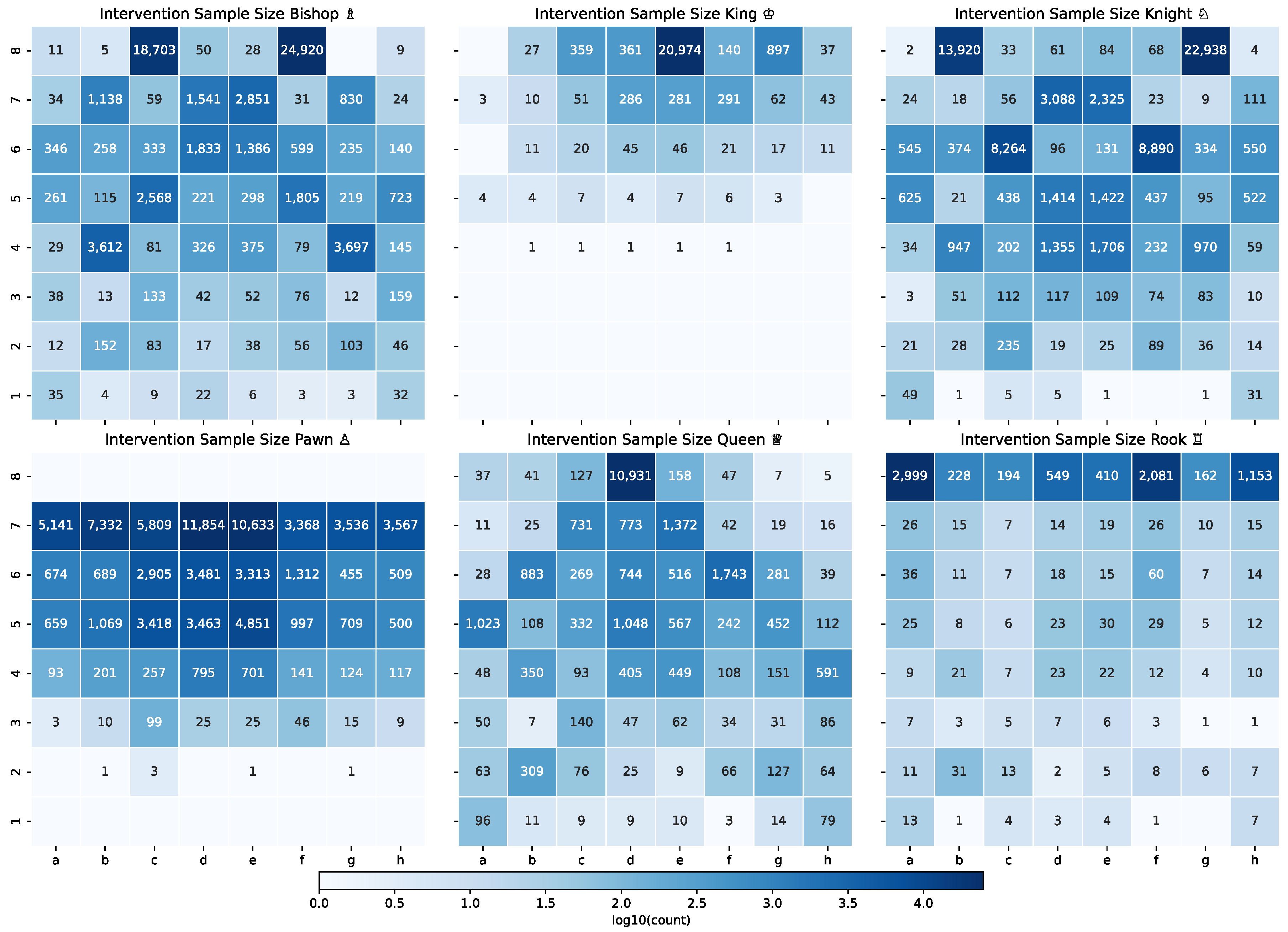
We pivoted the probe intervention data from Section 4.8 by square and piece type to see how intervening at different positions affects legal move rates. In aggregate, the results were uninteresting; however, when we look at interventions for a single-player (e.g., black), the interesting cases are easily discernable. So, in Figure 8, we show the mean success rate for black piece interventions only. (Per-square sample sizes are shown in Appendix C).
In Figure 8, each piece type is represented on a separate facet k, and the hue in each cell indicate mean LMPM for all interventions to remove piece k from square . Where the hue is pure white, no test case intervened against that square and piece type. Despite the large sample size (286k cases total), this is to be expected. For instance, the black king typically remains on the upper part of the chess board throughout the entire game. So, interventions against the black king were not sampled from first through fourth ranks (rows). Likewise, black pawns start on the 7th rank, they can only move forward, and they must immediately promote to another piece upon reaching the 1st rank. So, interventions against pawns on the first and eighth rank are simply impossible.
The interventions are consistently successful for most squares and piece types, with one notable exception: the interventions against the black queen at a1 (shown in red in Figure 8). In fact, the worst performance across all facets is concentrated on the queen interventions against the rank-1 squares. We hypothesize this is related to the fact that black pawns promote upon reaching one of the rank-1 squares and the difficulty the GPT had in predicting the rare tokens associated with pawn promotion.
4.11. Move Validity Post-Intervention with SAEs
Following the procedure in Section 4.8, we sampled output logits from an additional 403,848 interventions to evaluate our SAE-based probes. The output logits are partitioned based on the intervention applied, “None” is the control from the baseline forward pass of the GPT, “Probed_CD” uses the weights of the SAE-based contrastive difference probe, and “Probed_SAE” uses the weights of the linear probe trained on the SAE latent vectors. We applied softmax to the logits and report the LMPM according to the board position, either the original state or the target state. These results are summarized in Figure 9.
The GPT achieved a mean LMPM of 99.7% () according to the original board state (Figure 9, left). As a baseline for comparison, we grade the control “None” intervention against the target board state; it achieved a mean LMPM of 41.0% () in this setting (blue violin in Figure 9, right). This is to be expected. On average, the GPT allocates approximately 60% of the probability mass to its most-favored move. When the corresponding piece is removed, the entirety of that allocation is invalidated. The mass that remains valid does so only because there are multiple legal moves available in the overwhelming majority of board positions, and the GPT allocates some probability mass to those alternative moves.
Unfortunately, the SAE-based probes are only slightly better. A one-sided Welch’s t-test quantifies the standardized difference between the means of two groups. In this case, the test produced a p-value of for the SAE-based contrastive difference probe versus the control and a p-value of for the SAE-based linear probe versus the control. Although these small p-values allow us to conclude the increase in LMPM by the SAE-based probes is statistically significant, in practice the improvement is too small to meaningfully alter the model’s behavior or justify use of these SAE-based probes for residual stream editing.
A likely explanation for the SAE’s poor performance is not primarily information loss from sparsity, but rather the fact that SAEs are trained in an unsupervised fashion and therefore lack any mechanism for enforcing an ontologically coherent decomposition of the model’s latent space. During training, the SAE optimizes reconstruction quality under a sparsity penalty, but this objective does not necessarily align its learned features with domain-specific structure–in this case, the highly constrained ontology of chess piece identities, colors, board locations. As a result, the SAE often produces features that combine semantically unrelated components whenever such combinations reduce reconstruction error. A useful analogy is that the SAE behaves less like a careful disassembly of the model’s internal representations and more like an indiscriminate fragmentation process: it breaks the residual stream into parts that are convenient for minimizing its training objective, not parts that correspond to meaningful chess concepts. Because the SAE is not guided toward preserving the modularity inherent in chess (e.g., piece-type distinctions, spatial structure, turn order), we believe the resulting decomposition is poorly aligned with the ontology needed for effective representation editing.
5. Conclusions
This article advances the study of emergent representations in transformers through several key contributions. We release a chess-playing GPT model that improves upon the legal move rate of the LCB baseline and evaluate whether the hidden state representations honor the Markovian property of chess. We introduce a new evaluation metric–legal move probability mass (LMPM)–and use it to assess the intervention performance of probe classifiers trained on the original residual stream vs. ones trained on sparse autoencoder latents. The SAEs failed to reliably reconstruct board positions or support accurate causal interventions, suggesting that they did not capture the relevant emergent features of board state. Although SAEs may still hold value in certain interpretability contexts, our findings add to a growing body of evidence suggesting that, in some settings, they are no better–and sometimes markedly worse–than simpler techniques.
This pattern is consistent with some of the prior work in the area. In [47], SAEs trained on chess and Othello models capture some board-state information but still lag behind linear probes on supervised board reconstruction metrics, and [39] finds that SAE-based probes rarely outperform strong baselines trained directly on activations, winning on only a small subset of their 113 probing datasets. Moreover, [39] argues that some reported SAE gains in the literature may stem from weaker or mismatched baselines, for example, max-pooling activations across tokens in ways that hurt baseline performance, rather than from an intrinsic advantage of SAEs themselves. Taken together, these results suggest that for practitioners choosing between complex SAE pipelines and simpler linear probes, the latter will often provide comparable or superior performance at lower implementation and computational cost, unless there is a clear task-specific justification for the added complexity of SAEs.
This article also presents an analysis of the effect of model depth on probe classification vs. intervention performance. While F1 classification for linear probe classifiers peaks at layers 7 to 8, our findings show that intervention performance is highest between layers 3 to 7; applying interventions at deeper layers degrades the model’s ability to generate semantically valid moves. The broader implication is that intervention efficacy is non-linear across the depth of the model. Edits applied too early fail because the relevant information has not yet been encoded, and edits applied too late fail because the state has already been used in downstream computations. The key transferable insight is that the optimal intervention point is the layer where the model first establishes the predicate information being targeted—an idea that should generalize to other transformers, although the specific layer index will differ by domain and architecture.
We demonstrate that linear probes are highly interpretable: the weights of a probe trained to jointly classify piece type and color are well approximated by the sum of separate probes trained on type and color individually. However, a significant constraint of probe classifiers is their reliance on a priori concept definition. While selecting target features is trivial in bounded domains like chess—where game rules dictate clear concepts—it becomes increasingly difficult in the open-ended landscape of natural language, where the space of plausible concepts is vast. Consequently, our future research will focus on developing unsupervised methods that can automatically discover relevant concepts using external data, removing the bottleneck of manual selection.
Author Contributions
Conceptualization, A.D. and G.S.; software, A.D; investigation, A.D. and R.V.; writing—original draft preparation, A.D. and R.V.; writing—review and editing, G.S.; visualization, A.D.; data curation, A.D.; supervision, G.S.; resources, G.S. All authors have read and agreed to the published version of the manuscript.
Funding
This research received no external funding.
Data Availability Statement
The source code, GPT model, training data, probe classifiers, and SAEs are available online at: https://github.com/austinleedavis/icmla-2024
Acknowledgments
During the preparation of this manuscript/study, the author(s) used Gemini 2.5 and 3 for grammar correction and sentence restructuring. The authors have reviewed and edited the output and take full responsibility for the content of this publication.
Conflicts of Interest
The authors declare no conflicts of interest.
Abbreviations
The following abbreviations are used in this manuscript:
| CD | Contrastive Difference |
| GPT | Generative Pre-trained Transformer |
| LLM | Large Language Model |
| LMPM | Legal Move Probability Mass |
| MSE | Mean Squared Error |
| PEFT | Parameter Efficient Fine Tuning |
| SAE | Sparse Autoencoders |
| UCI | Universal Chess Interface |
Appendix A. Chess Terminology and Notation
In chess, a move consists of both a player’s action and the opponent’s subsequent response, while a ply refers to a single action by one player. We call a sequence of chess moves the trace and denote it with . Throughout this paper, the reader can assume the trace is a sequence of encoded token indices. All traces are converted to UCI notation, a space-delimited format wherein each player’s turn (“ply”) is represented by (up to) three parts: the starting square, the ending square, and (occasionally) the pawn promotion type. For example, a pawn promotion to a queen by moving from b7 to b8 is written in UCI notation as “b7b8q”, and a knight moving from b1 to c3 is written as “b1c3”.
Appendix B. Tokenization and GPT Training Details
The UCI move sequences were tokenized by splitting each ply into up to three phases. For instance, the UCI string “b7b8q b1c3” becomes [bos, b7, b8, q, b1, c3], where bos is the special beginning of string token.
The game trace is obtained by replacing these tokens with indices from the vocabulary. We used a vocabulary with 72 tokens (see Table A1). Except for special tokens (which are ignored during evaluation), this tokenization scheme matches that of the LCB model [35].

Table A1.
Model Vocabulary.
| Type | Examples | Count |
|---|---|---|
| Special symbols | bos, eos, pad, unk | 4 |
| Square names | a1, e4, h8 | 64 |
| Pawn promotion type | n, b, r, q | 4 |
| Total | 72 |
The GPT was trained from scratch, i.e., weights were randomly initialized before training. Once training was complete, the weights of the GPT model were fixed and unchanged throughout our analysis. The training parameters are shown in Table A2.
Table A2.
Training Parameters for GPT.
| Parameter | Value |
|---|---|
| block size | 512 |
| initial learning rate | 2e-4 |
| weight decay | 0.01 |
| learning rate scheduler | cosine |
| optimizer | Adam |
| Adam , | (0.9, 0.999) |
| Adam | 1e-8 |
| batch size | 6 |
| epochs | 1 |
| max_grad_norm | 1.0 |
| bf16 | true |
Appendix C. Per-Square Intervention Count
In Section 4.10, we discussed how performance of the linear probes varied across the squares on the chess board, noting that some positions are more common than others. The figure below shows the number of interventions against black’s pieces in the underlying dataset. The individual squares are labeled using the raw count of interventions against a given piece on a given square. We apply a log scale to the cell colors since the distribution of counts varies over several orders of magnitude. Interventions were most common against the pieces’ starting positions. The number of interventions does not correlate with the LMPM of the intervention. For instance, Figure A1 shows LMPM for interventions against a black Bishop on B7 was substantially lower than for B6, despite B6 having considerably fewer samples.
Figure A1.
Intervention counts by-square. The figure shows the number of interventions performed against black player’s pieces located on each square on the board.
Figure A1.
Intervention counts by-square. The figure shows the number of interventions performed against black player’s pieces located on each square on the board.
Appendix D. Probe Training
The results of [48] indicated their GPT learned an ego-centric representation for moves in the game of Othello, i.e., “my turn“ and “your turn“ rather than “white’s turn“ and “black’s turn“. However, unlike Othello, the strategies for black and white players in chess are vastly different. So, rather than treating each turn in an ego-centric way, our tokenization scheme supported five distinct phases for each whole move:
- Phase : white start square
- Phase : white end square
- Phase : black start square
- Phase : black end square
- Phase : white or black promotions
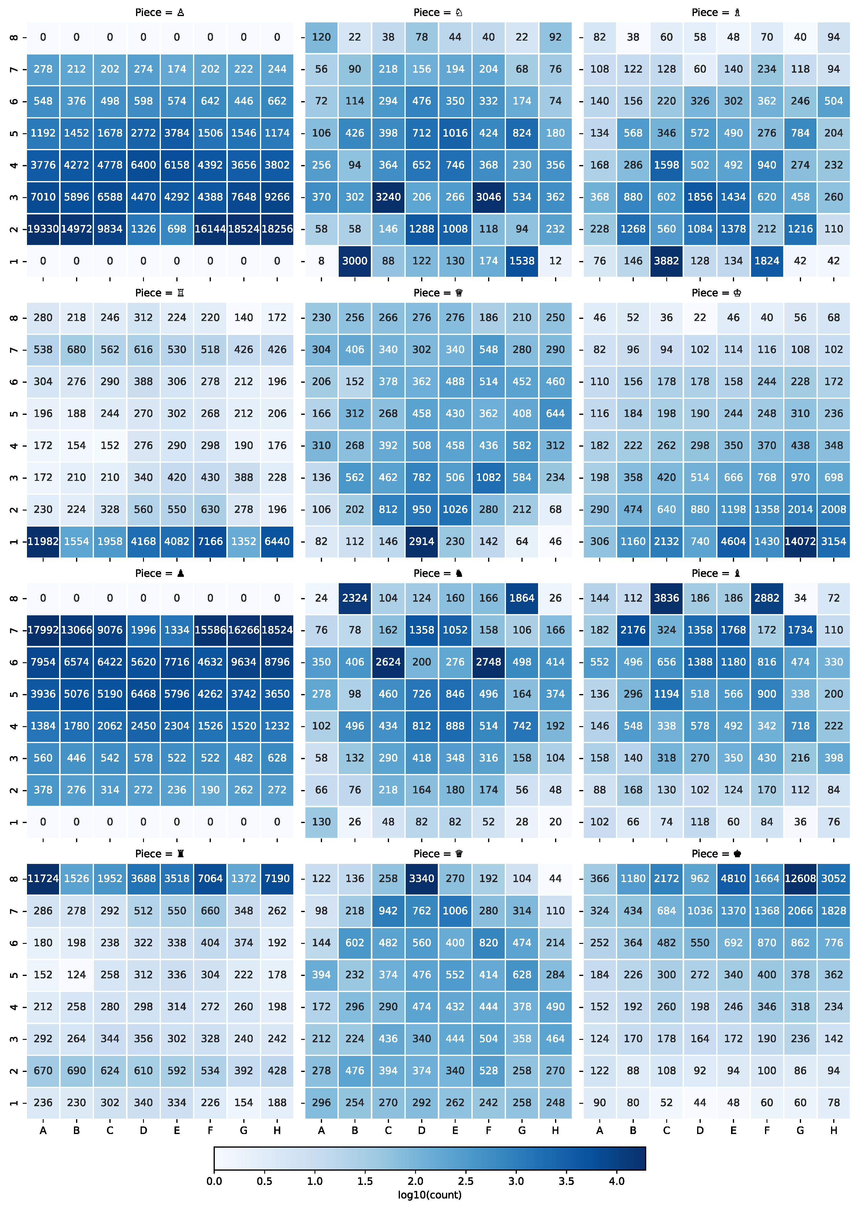
While training linear probes, we limited each probe’s training data to a single phase, i.e., we trained five distinct probes for each square and layer. The training dataset for a single phase’s probe consisted of a single board position from each phase of each of the 120k games played in January 2013 and published in the Lichess.org open database. Figure A2 shows the number of times a given piece appeared on each square within the probe training dataset used to perform our interventions.
We trained the linear probes on a 16-core NVIDIA GeForce RTX 3060 Laptop GPU. Training for a single layer-phase takes approximately 8 minutes so training a complete suite of linear probes across all 12 layers and 5 phases takes approximately 8 hours. The linear probe training parameters are listed in Table A3.
Table A3.
Training Parameters for Linear Probes.
| Parameter | Value |
|---|---|
| initial learning rate | 9e-3 |
| learning rate scheduler | cosine |
| weight decay | 0.01 |
| optimizer | AdamW |
| Adam , | (0.9, 0.999) |
| Adam | 1e-8 |
| batch size | 2,000 |
| epochs | 20 |
| max_grad_norm | 1.0 |
Figure A2.
Piece count by square within probe training data. The figure shows the number of times each piece type was observed on each square of the board within the training data for a single phase probe–the same probe used to intervene against black pieces above.
Figure A2.
Piece count by square within probe training data. The figure shows the number of times each piece type was observed on each square of the board within the training data for a single phase probe–the same probe used to intervene against black pieces above.
References
- Minaee, S.; Mikolov, T.; Nikzad, N.; Chenaghlu, M.; Socher, R.; Amatriain, X.; Gao, J. Large Language Models: A Survey. arXiv 2024, arXiv:2402.06196. [Google Scholar]
- Li, J.; Consul, S.; Zhou, E.; Wong, J.; Farooqui, N.; Ye, Y.; Manohar, N.; Wei, Z.; Wu, T.; Echols, B.; et al. Banishing LLM Hallucinations Requires Rethinking Generalization. arXiv 2024, arXiv:2406.17642. [Google Scholar] [CrossRef]
- McGrath, T.; Kapishnikov, A.; Tomašev, N.; Pearce, A.; Wattenberg, M.; Hassabis, D.; Kim, B.; Paquet, U.; Kramnik, V. Acquisition of Chess Knowledge in AlphaZero. Proceedings of the National Academy of Sciences 2022, 119, e2206625119. [Google Scholar] [CrossRef]
- Silver, D.; Hubert, T.; Schrittwieser, J.; Antonoglou, I.; Lai, M.; Guez, A.; Lanctot, M.; Sifre, L.; Kumaran, D.; Graepel, T.; et al. Mastering Chess and Shogi by Self-Play with a General Reinforcement Learning Algorithm. arXiv 2017, arXiv:1712.01815. [Google Scholar] [CrossRef]
- Silver, D.; Schrittwieser, J.; Simonyan, K.; Antonoglou, I.; Huang, A.; Guez, A.; Hubert, T.; Baker, L.; Lai, M.; Bolton, A.; et al. Mastering the Game of Go without Human Knowledge. Nature 2017, 550, 354–359. [Google Scholar] [CrossRef]
- Vinyals, O.; Babuschkin, I.; Czarnecki, W.M.; Mathieu, M.; Dudzik, A.; Chung, J.; Choi, D.H.; Powell, R.; Ewalds, T.; Georgiev, P.; et al. Grandmaster Level in StarCraft II Using Multi-Agent Reinforcement Learning. Nature 2019, 575, 350–354. [Google Scholar] [CrossRef] [PubMed]
- Davis, A.; Sukthankar, G. Performance Envelopes of Linear Probes for Latent Representation Edits in Gpt Models. In Proceedings of the 2024 International Conference on Machine Learning and Applications (ICMLA), Coral Gables, FL, USA, 18–20 December 2024. [Google Scholar]
- Lialin, V.; Deshpande, V.; Rumshisky, A. Scaling down to Scale up: A Guide to Parameter-Efficient Fine-Tuning. arXiv 2023, arXiv:2303.15647. [Google Scholar] [CrossRef]
- Li, X.L.; Liang, P. Prefix-Tuning: Optimizing Continuous Prompts for Generation. arXiv 2021, arXiv:2101.00190. [Google Scholar] [CrossRef]
- Hu, E.J.; Shen, Y.; Wallis, P.; Allen-Zhu, Z.; Li, Y.; Wang, S.; Wang, L.; Chen, W. LoRA: Low-rank Adaptation of Large Language Models. arXiv 2021, arXiv:2106.09685. [Google Scholar]
- Christiano, P.F.; Leike, J.; Brown, T.; Martic, M.; Legg, S.; Amodei, D. Deep Reinforcement Learning from Human Preferences. Advances in Neural Information Processing Systems 2017, 30, 4302–4310. [Google Scholar]
- Ouyang, L.; Wu, J.; Jiang, X.; Almeida, D.; Wainwright, C.L.; Mishkin, P.; Zhang, C.; Agarwal, S.; Slama, K.; Ray, A.; et al. Training language models to follow instructions with human feedback. In Proceedings of the Advances in Neural Information Processing Systems; Koyejo, S., Mohamed, S., Agarwal, A., Belgrave, D., Cho, K., Oh, A., Eds.; Curran Associates, Inc.: Red Hook, NY, USA, 2022; Volume 35, pp. 27730–27744. [Google Scholar]
- Zou, A.; Phan, L.; Chen, S.; Campbell, J.; Guo, P.; Ren, R.; Pan, A.; Yin, X.; Mazeika, M.; Dombrowski, A.K.; et al. Representation Engineering: A Top-down Approach to AI Transparency, 2023. arXiv 2023, arXiv:2310.01405. [Google Scholar]
- Nanda, N. A Comprehensive Mechanistic Interpretability Explainer and Glossary.
- Meng, K.; Bau, D.; Andonian, A.; Belinkov, Y. Locating and Editing Factual Associations in GPT. In Proceedings of the Advances in Neural Information Processing Systems; Koyejo, S., Mohamed, S., Agarwal, A., Belgrave, D., Cho, K., Oh, A., Eds.; Curran Associates, Inc.: Red Hook, NY, USA, 2022; Volume 35, pp. 17359–17372. [Google Scholar]
- Elhage, N.; Nanda, N.; Olsson, C.; Henighan, T.; Joseph, N.; Mann, B.; Askell, A.; Bai, Y.; Chen, A.; Conerly, T.; et al. A Mathematical Framework for Transformer Circuits. Transformer Circuits Thread 2021, 1, 12. [Google Scholar]
- Wang, K.R.; Variengien, A.; Conmy, A.; Shlegeris, B.; Steinhardt, J. Interpretability in the Wild: A Circuit for Indirect Object Identification in GPT-2 Small. In Proceedings of the Eleventh International Conference on Learning Representations, Kigali, Rwanda, 1–5 May 2023. [Google Scholar]
- Conmy, A.; Mavor-Parker, A.; Lynch, A.; Heimersheim, S.; Garriga-Alonso, A. Towards Automated Circuit Discovery for Mechanistic Interpretability. Advances in Neural Information Processing Systems 2023, 36, 16318–16352. [Google Scholar]
- Rimsky, N.; Gabrieli, N.; Schulz, J.; Tong, M.; Hubinger, E.; Turner, A.M. Steering Llama 2 via contrastive activation addition. arXiv 2023, arXiv:2312.06681. [Google Scholar]
- Park, K.; Choe, Y.J.; Veitch, V. The linear representation hypothesis and the geometry of large language models. arXiv 2023, arXiv:2311.03658. [Google Scholar] [CrossRef]
- Alain, G.; Bengio, Y. Understanding intermediate layers using linear classifier probes. arXiv 2016, arXiv:1610.01644. [Google Scholar]
- Hewitt, J.; Liang, P. Designing and Interpreting Probes with Control Tasks. In Proceedings of the 2019 Conference on Empirical Methods in Natural Language Processing and the 9th International Joint Conference on Natural Language Processing (EMNLP-IJCNLP), Hong Kong, China, 3–7 November 2019; 2019; pp. 2733–2743. [Google Scholar]
- Belinkov, Y.; Màrquez, L.; Sajjad, H.; Durrani, N.; Dalvi, F.; Glass, J. Evaluating layers of representation in neural machine translation on part-of-speech and semantic tagging tasks. arXiv 2018, arXiv:1801.07772. [Google Scholar]
- Belinkov, Y. Probing Classifiers: Promises, Shortcomings, and Advances. Computational Linguistics 2022, 48, 207–219. [Google Scholar] [CrossRef]
- Bricken, T.; Templeton, A.; Batson, J.; Chen, B.; Jermyn, A.; Conerly, T.; Turner, N.; Anil, C.; Denison, C.; Askell, A.; et al. Towards Monosemanticity: Decomposing Language Models With Dictionary Learning. Transformer Circuits Thread 2023.
- Conerly, T.; Templeton, A.; Bricken, T.; Marcus, J.; Henighan, T. Circuits Updates - April 2024—Transformer-Circuits.Pub, 2024.
- Rajamanoharan, S.; Conmy, A.; Smith, L.; Lieberum, T.; Varma, V.; Kramár, J.; Shah, R.; Nanda, N. Improving Dictionary Learning with Gated Sparse Autoencoders. arXiv 2024, arXiv:2404.16014. [Google Scholar] [CrossRef]
- Gao, L.; la Tour, T.D.; Tillman, H.; Goh, G.; Troll, R.; Radford, A.; Sutskever, I.; Leike, J.; Wu, J. Scaling and Evaluating Sparse Autoencoders. arXiv 2024, arXiv:2406.04093. [Google Scholar] [CrossRef]
- Bussmann, B.; Leask, P.; Nanda, N. Learning Multi-Level Features with Matryoshka Saes, 2024.
- Karvonen, A.; Wright, B.; Rager, C.; Angell, R.; Brinkmann, J.; Smith, L.; Verdun, C.M.; Bau, D.; Marks, S. Measuring Progress in Dictionary Learning for Language Model Interpretability with Board Game Models. arXiv 2024, arXiv:2408.00113. [Google Scholar] [CrossRef]
- Bussmann, B.; Leask, P.; Nanda, N. BatchTopK Sparse Autoencoders. arXiv 2024, arXiv:2412.06410. [Google Scholar]
- Li, K.; Hopkins, A.K.; Bau, D.; Viégas, F.; Pfister, H.; Wattenberg, M. Emergent World Representations: Exploring a Sequence Model Trained on a Synthetic Task. In Proceedings of the International Conference on Learning Representations, Kigali, Rwanda, 1–5 May 2023. [Google Scholar]
- Nanda, N.; Lee, A.; Wattenberg, M. Emergent Linear Representations in World Models of Self-Supervised Sequence Models. In Proceedings of the 6th BlackboxNLP Workshop: Analyzing and Interpreting Neural Networks for NLP, Singapore, 7 December 2023; pp. 16–30. [Google Scholar] [CrossRef]
- Karvonen, A.; Wright, B.; Rager, C.; Angell, R.; Brinkmann, J.; Smith, L.; Verdun, C.M.; Bau, D.; Marks, S. Measuring Progress in Dictionary Learning for Language Model Interpretability with Board Game Models. arXiv 2024, arXiv:2408.00113. [Google Scholar] [CrossRef]
- Toshniwal, S.; Wiseman, S.; Livescu, K.; Gimpel, K. Chess as a Testbed for Language Model State Tracking. Proceedings of the AAAI Conference on Artificial Intelligence 2022, 36, 11385–11393. [Google Scholar] [CrossRef]
- Karvonen, A. Emergent World Models and Latent Variable Estimation in Chess-Playing Language Models. In Proceedings of the First Conference on Language Modeling, Philadelphia, PA, USA, 7–9 October 2024. [Google Scholar]
- Davis, A.L.; Sukthankar, G. Decoding Chess Mastery: A Mechanistic Analysis of a Chess Language Transformer Model. In Artificial General Intelligence; Thórisson, K.R., Isaev, P., Sheikhlar, A., Eds.; Springer: Cham, Switzerland, 2024; Volume 14951, pp. 63–72. [Google Scholar] [CrossRef]
- Houlsby, N.; Giurgiu, A.; Jastrzebski, S.; Morrone, B.; De Laroussilhe, Q.; Gesmundo, A.; Attariyan, M.; Gelly, S. Parameter-Efficient Transfer Learning for NLP. In Proceedings of the International Conference on Machine Learning, Long Beach, CA, USA, 10–15 June 2019; pp. 2790–2799. [Google Scholar]
- Kantamneni, S.; Engels, J.; Rajamanoharan, S.; Tegmark, M.; Nanda, N. Are Sparse Autoencoders Useful? A Case Study in Sparse Probing. arXiv 2025, arXiv:2502.16681. [Google Scholar] [CrossRef]
- The LCZero Authors. LeelaChessZero.
- Solaiman, I. Release Strategies and the Social Impacts of Language Models. arXiv 2019, arXiv:1908.09203. [Google Scholar] [CrossRef]
- Feng, X.; Luo, Y.; Wang, Z.; Tang, H.; Yang, M.; Shao, K.; Mguni, D.H.; Du, Y.; Wang, J. ChessGPT: Bridging Policy Learning and Language Modeling. In Proceedings of the Thirty-Seventh Conference on Neural Information Processing Systems Datasets and Benchmarks Track, New Orleans, LA, USA, 10–16 December 2023. [Google Scholar]
- Barnes, D.J. Pgn-Extract. University of Kent, 2023.
- Fiotto-Kaufman, J.; Loftus, A.R.; Todd, E.; Brinkmann, J.; Juang, C.; Pal, K.; Rager, C.; Mueller, A.; Marks, S.; Sharma, A.S.; et al. NNsight and NDIF: Democratizing Access to Foundation Model Internals. arXiv 2024, arXiv:2407.14561. [Google Scholar] [CrossRef]
- Nanda, N.; Bloom, J. TransformerLens. 2022. Available online: https://github.com/TransformerLensOrg/TransformerLens.
- Ansel, J. PyTorch 2: Faster Machine Learning through Dynamic Python Bytecode Transformation and Graph Compilation. In Proceedings of the 29th ACM ASPLOS, La Jolla, CA, USA, 27 April–1 May 2024. [Google Scholar] [CrossRef]
- Karvonen, A.; Wright, B.; Rager, C.; Angell, R.; Brinkmann, J.; Smith, L.; Verdun, C.M.; Bau, D.; Marks, S. Measuring Progress in Dictionary Learning for Language Model Interpretability with Board Game Models. arXiv 2024, arXiv:2408.00113. [Google Scholar] [CrossRef]
- Nanda, N.; Lee, A.; Wattenberg, M. Emergent Linear Representations in World Models of Self-Supervised Sequence Models. In Proceedings of the 6th BlackboxNLP Workshop: Analyzing and Interpreting Neural Networks for NLP; Belinkov, Y., Hao, S., Jumelet, J., Kim, N., McCarthy, A., Mohebbi, H., Eds.; Association for Computational Linguistics: Stroudsburg, PA, USA; pp. 16–30.
Figure 1.
Two methods for building linear probes using trained Sparse Autoencoders. Top: A probe maps SAE-encoded GPT hidden states to the board state at each move—same as standard probe training, but inputs are first encoded by the SAE. The final weights are decoded by the SAE so they match the shape of the residual stream. Bottom: Residual stream vectors from 10,000 games are SAE-encoded. For each feature j, vectors are grouped by whether j is active on the board. The probe weight is the difference of means between these groups for each feature and layer.
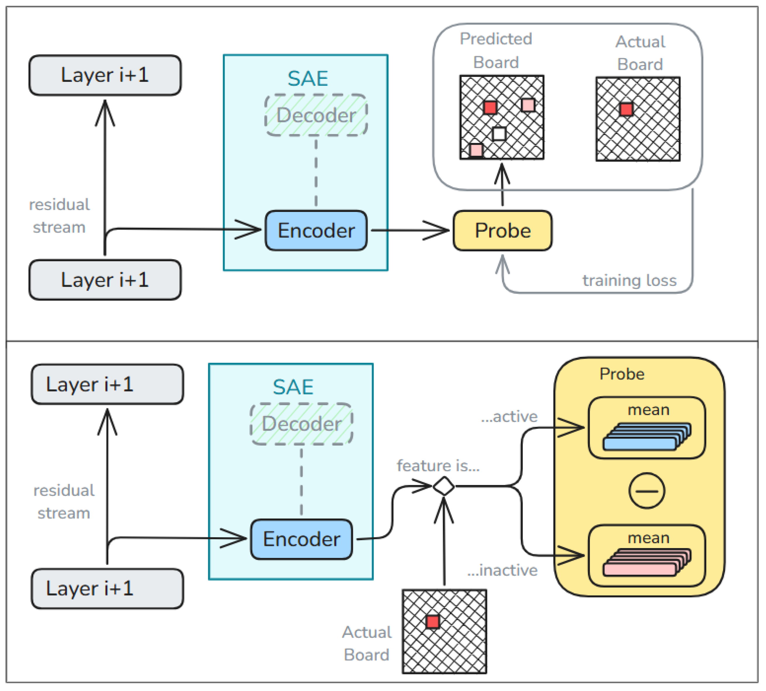
Figure 2.
Legal move probability mass post-intervention for different values of . Values are averaged over 500 random games of chess.
Figure 2.
Legal move probability mass post-intervention for different values of . Values are averaged over 500 random games of chess.
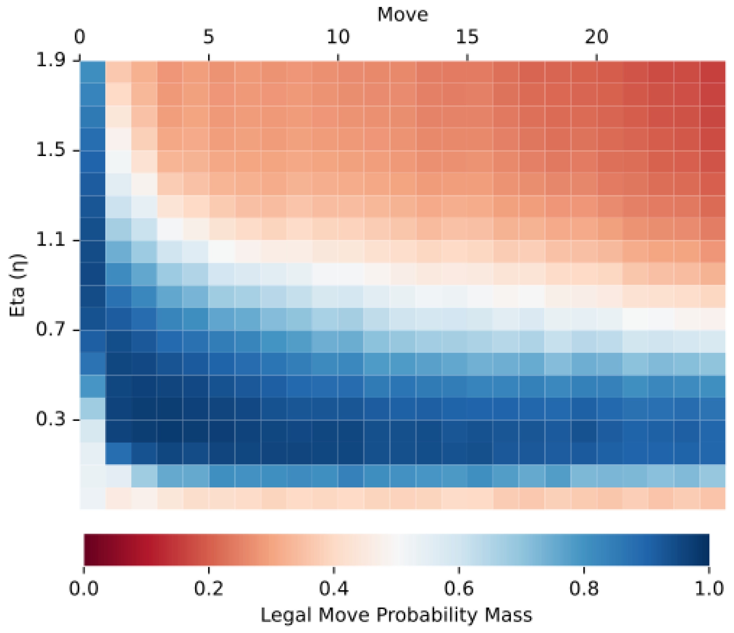
Figure 3.
Example Board Positions. TL: Game trace produces the Original State board position in the top left. The green arrow indicates GPT’s pre-intervention suggestion to move the bishop from c1 to h6. TR: The probe intervention will remove the c1 bishop from the board as depicted in the top right quadrant. BL: The target board resulting from removing the c1 bishop is shown in the bottom left; the green arrow indicates the GPT’s post-intervention suggestion to move the knight from g1 to f3. BR: The bottom right shows the future board which represents the board position six tokens beyond the intervention position i.
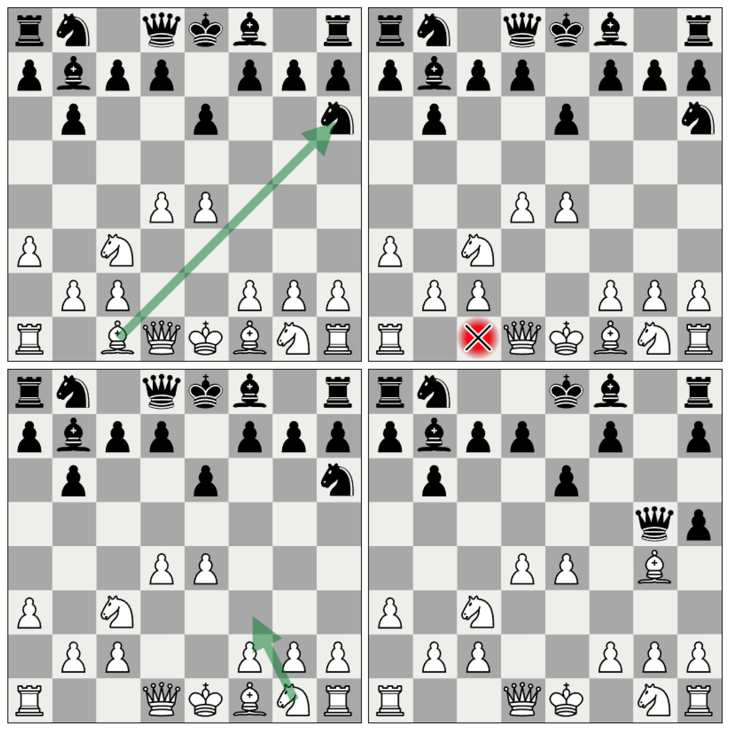
Figure 4.
Cosine similarity between the column vectors of the main probe weight matrix and the linear combination of column vectors from the color and piece probes. Each facet relates to a single column vector k from our probe which classifies color and piece type simultaneously. For each facet k, the value in cell indicates the cosine similarity between the kth column of the main probe versus the sum of the ith column of the color probe and the jth column vector of the piece type probe. Specifically, . The highest values occur exactly at the cells at the intersection of the row and column corresponding with the facet class, indicating the joint representation for (piece, color) can be decomposed into two separate representations: one for piece and one for color.
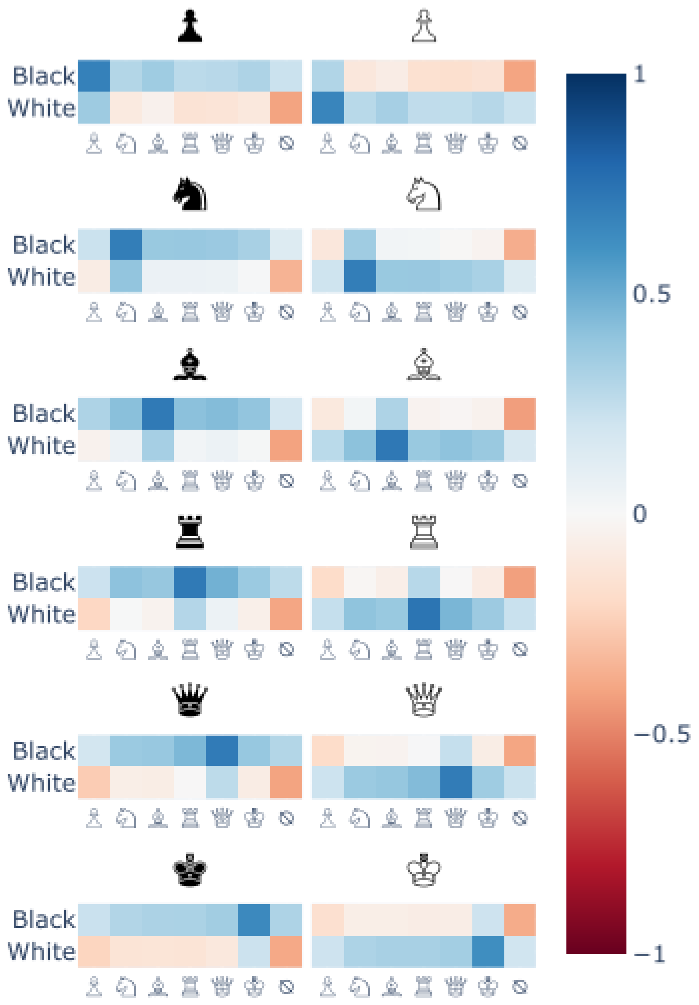
Figure 5.
An example intervention that switches a Scandinavian Defense opening to a King’s Pawn opening. A heatmap of the GPT outputs are shown at the bottom. Pre-intervention, the GPT recommends taking the black pawn on d6. Post-intervention, the e4 pawn has no legal moves. So, the GPT recommends moving the d2 pawn or g1 knight instead.
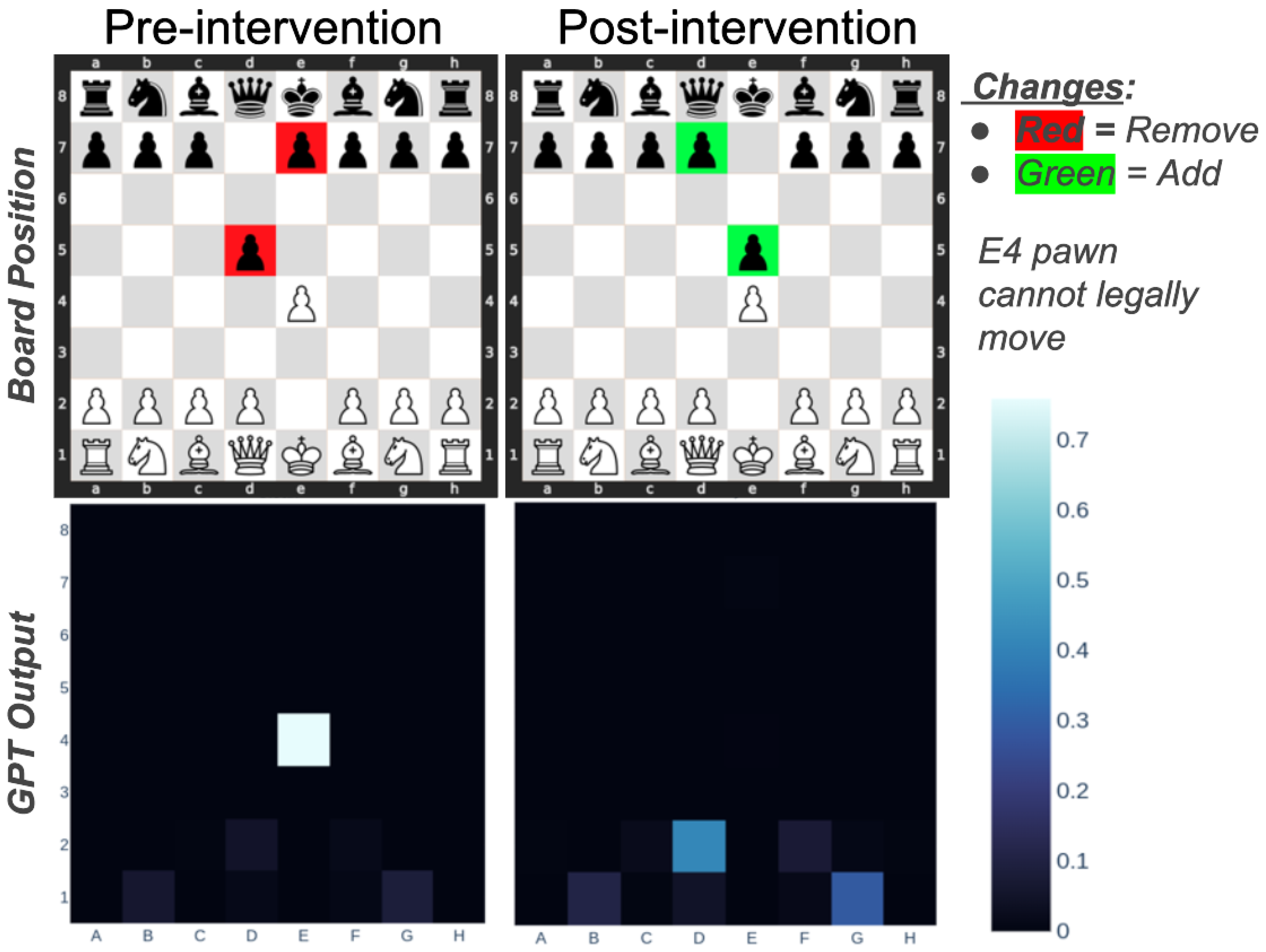
Figure 6.
Legal Move Probability Mass distributions computed for interventions assuming either the Original (left), Target (center), or Future (right) board positions. The intervention vector type is listed on the horizontal axis.
Figure 6.
Legal Move Probability Mass distributions computed for interventions assuming either the Original (left), Target (center), or Future (right) board positions. The intervention vector type is listed on the horizontal axis.
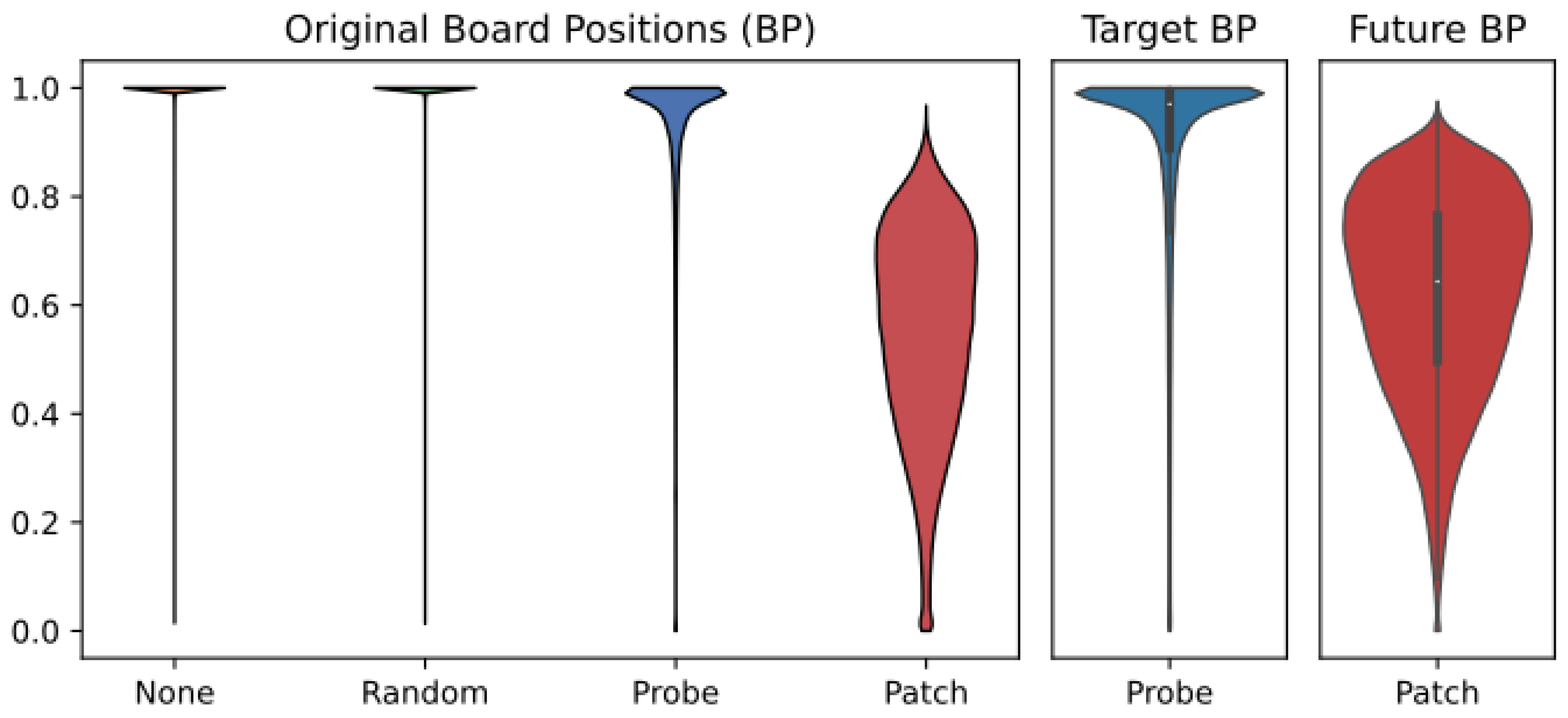
Figure 7.
Probability mass for valid moves post-intervention by-layer. Median values are shown with a black dot, and the nested blue rectangles indicate the 50%, 80%, and 95% inner-quantile ranges with progressively lighter shades.
Figure 7.
Probability mass for valid moves post-intervention by-layer. Median values are shown with a black dot, and the nested blue rectangles indicate the 50%, 80%, and 95% inner-quantile ranges with progressively lighter shades.
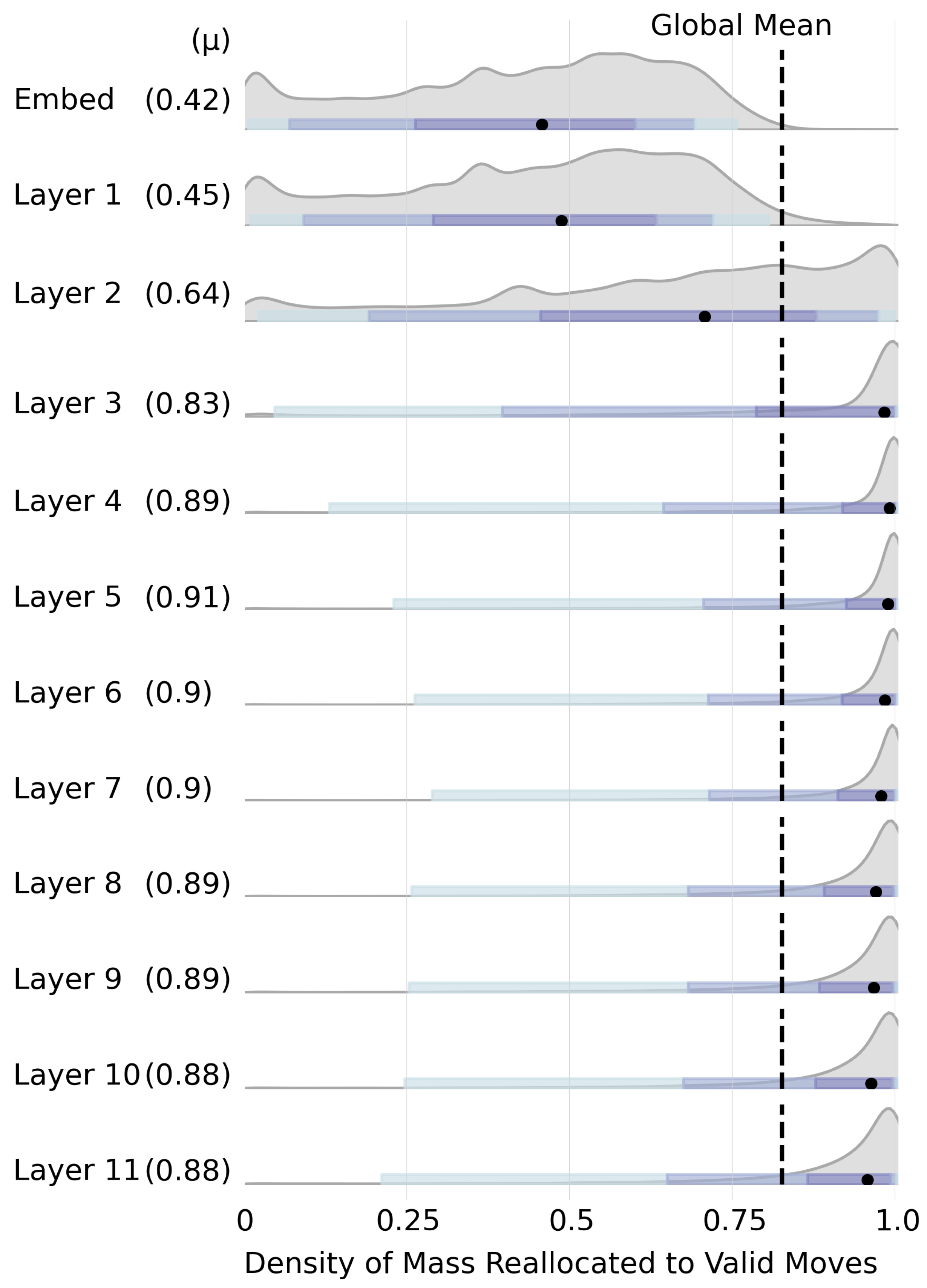
Figure 8.
Mean success rate by location for black piece interventions. Each facet shows mean probe success rate for the given piece type according to the position affected by the intervention. Blank cells indicate of the 286k black-piece interventions, none targeted that (square, piece type) combination.
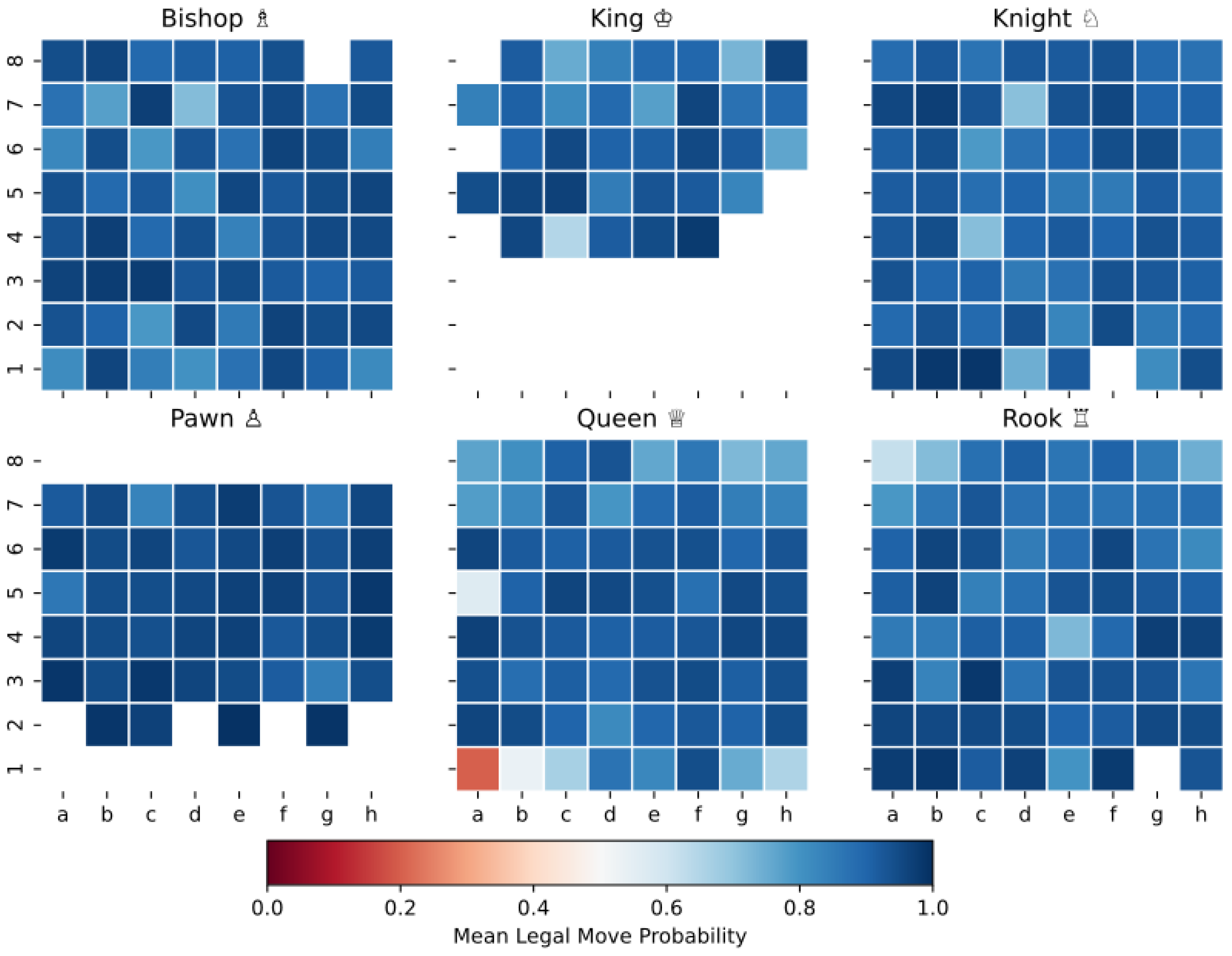
Figure 9.
Legal Move Probability Mass distributions computed for interventions assuming either the Original (left) or Target (right) board positions. The intervention vector type is listed on the horizontal axis.
Figure 9.
Legal Move Probability Mass distributions computed for interventions assuming either the Original (left) or Target (right) board positions. The intervention vector type is listed on the horizontal axis.
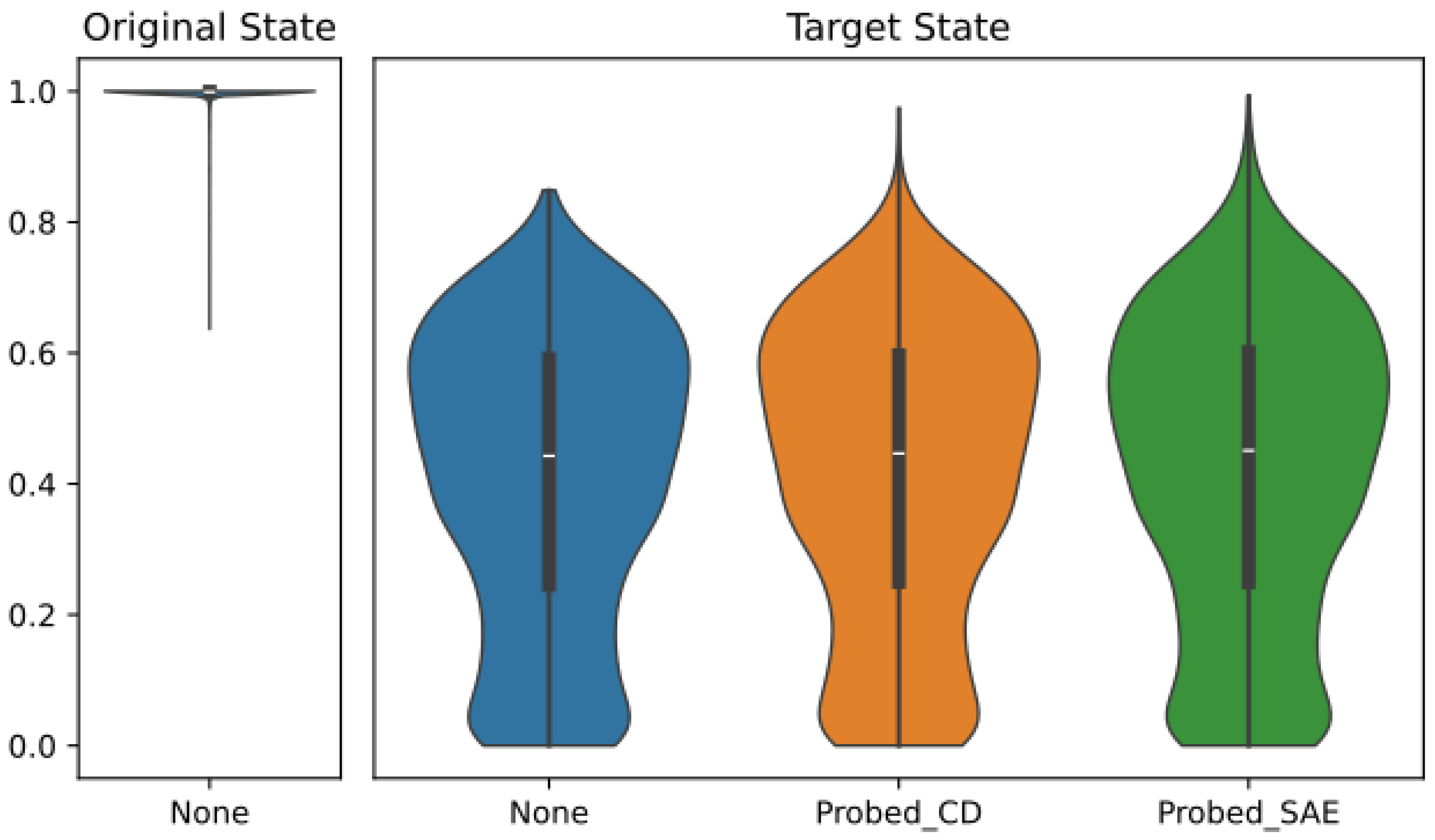
Table 1.
Overview of Related Work.
| Fine Tuning | [8,9,10,11,12] |
| Model Transparency | [13,14,15,16,17,18,19] |
| Linear Representations | [20] |
| Probe Classifiers | [21,22,23,24] |
| Sparse Auto Encoders | [25,26,27,28,29,30,31] |
| Emergent World Models | [32,33,34,35,36,34,37] |
Table 2.
Chess GPT Performance.
| Metric | Ours | LCB [35] | 16-layer [36] | 8-layer [36] |
|---|---|---|---|---|
| Perplexity | 2.262 | 3.486 | - | - |
| Top-1 Acc (%) | 71.3 | 60.4 | - | - |
| Top-5 Acc (%) | 97.3 | 93.9 | - | - |
| Legal Rate (%) | 99.9 | 97.7 | 99.8 | 99.6 |
Table 3.
SAE Performance Metrics.
| Metric | Mean | Std | Min | Max |
|---|---|---|---|---|
| Cross-Entropy Loss with SAE | 1.19 | 0.16 | 1.03 | 1.49 |
| Cross-Entropy Loss Increase | 0.25 | 0.16 | 0.09 | 0.55 |
| Cross-Entropy Loss Score | 0.95 | 0.04 | 0.89 | 0.98 |
| Sparsity (L0 norm) | 14.35 | 4.09 | 10.01 | 20.08 |
| Sparsity (L1 norm) | 24.63 | 8.26 | 15.68 | 35.5 |
| Reconstruction MSE | 0.14 | 0.12 | 0.02 | 0.39 |
| Reconstruction Cosine Similarity | 0.97 | 0.02 | 0.93 | 1.0 |
Table 4.
SAE-based Probe Board Position Classification Performance.
| Layer (ℓ) | Accuracy | F1 | Precision | Recall |
|---|---|---|---|---|
| 1 | 0.77 | 0.72 | 0.74 | 0.77 |
| 2 | 0.78 | 0.74 | 0.75 | 0.78 |
| 3 | 0.78 | 0.73 | 0.75 | 0.78 |
| 4 | 0.78 | 0.74 | 0.76 | 0.78 |
| 5 | 0.78 | 0.74 | 0.76 | 0.78 |
| 6 | 0.79 | 0.76 | 0.77 | 0.79 |
| 7 | 0.81 | 0.79 | 0.79 | 0.81 |
| 8 | 0.84 | 0.83 | 0.83 | 0.84 |
| 9 | 0.87 | 0.86 | 0.87 | 0.87 |
| 10 | 0.88 | 0.88 | 0.88 | 0.88 |
| 11 | 0.87 | 0.86 | 0.86 | 0.87 |
| 12 | 0.87 | 0.87 | 0.87 | 0.87 |
Table 5.
Linear Probe Board Position Classification Performance.
| Layer (ℓ) | Accuracy | F1 | Precision | Recall |
|---|---|---|---|---|
| Embed | 0.78 | 0.73 | 0.74 | 0.78 |
| 1 | 0.82 | 0.79 | 0.81 | 0.82 |
| 2 | 0.85 | 0.82 | 0.84 | 0.85 |
| 3 | 0.90 | 0.88 | 0.89 | 0.90 |
| 4 | 0.92 | 0.91 | 0.91 | 0.92 |
| 5 | 0.93 | 0.92 | 0.93 | 0.93 |
| 6 | 0.95 | 0.94 | 0.94 | 0.95 |
| 7 | 0.95 | 0.95 | 0.94 | 0.95 |
| 8 | 0.95 | 0.95 | 0.94 | 0.95 |
| 9 | 0.94 | 0.94 | 0.93 | 0.94 |
| 10 | 0.93 | 0.93 | 0.93 | 0.93 |
| 11 | 0.93 | 0.93 | 0.93 | 0.93 |
| 12 | 0.94 | 0.93 | 0.94 | 0.94 |
Table 6.
Markovian test statistics by layer.
| Layer | Cohen’s d | |||
|---|---|---|---|---|
| 0 | 3.20e-07 | 0.0427 | 0.0114 | 0.4838 |
| 1 | 9.36e-05 | 0.2414 | 0.0304 | 0.9855 |
| 2 | 7.96e-04 | 0.2196 | 0.0284 | 0.9633 |
| 3 | -4.46e-04 | 0.2911 | 0.0357 | 1.0205 |
| 4 | 6.24e-04 | 0.4013 | 0.0257 | 1.8752 |
| 5 | -1.97e-05 | 0.4382 | 0.0212 | 2.5462 |
| 6 | -3.07e-04 | 0.4853 | 0.0153 | 3.6095 |
| 7 | 6.96e-04 | 0.5352 | 0.0125 | 5.0553 |
| 8 | -9.20e-05 | 0.5792 | 0.0111 | 6.3650 |
| 9 | -5.89e-05 | 0.6024 | 0.0106 | 7.0107 |
| 10 | 2.28e-04 | 0.6345 | 0.0114 | 7.2777 |
| 11 | 9.56e-05 | 0.6657 | 0.0127 | 6.9736 |
| 12 | -9.38e-06 | 0.7049 | 0.0074 | 7.5987 |
Disclaimer/Publisher’s Note: The statements, opinions and data contained in all publications are solely those of the individual author(s) and contributor(s) and not of MDPI and/or the editor(s). MDPI and/or the editor(s) disclaim responsibility for any injury to people or property resulting from any ideas, methods, instructions or products referred to in the content. |
© 2026 by the authors. Licensee MDPI, Basel, Switzerland. This article is an open access article distributed under the terms and conditions of the Creative Commons Attribution (CC BY) license (http://creativecommons.org/licenses/by/4.0/).
Copyright: This open access article is published under a Creative Commons CC BY 4.0 license, which permit the free download, distribution, and reuse, provided that the author and preprint are cited in any reuse.


