
Submitted:
23 December 2025
Posted:
24 December 2025
You are already at the latest version
Abstract
Empirical debates about a "crisis of trust'' highlight long-lived pockets of high trust and deep distrust in institutions, as well as abrupt, shock-induced shifts between them. We propose a probabilistic model in which such phenomena emerge endogenously from social learning on hierarchical networks. Starting from a discrete model on a directed acyclic graph, where each agent makes a binary adoption decision about a single assertion, we derive an effective influence kernel that maps individual priors to stationary adoption probabilities. A continuum limit along hierarchical depth yields a degenerate, non-conservative logistic--diffusion equation for the adoption probability u(x,t), in which diffusion is modulated by (1-u) and increases the integral of u rather than preserving it. To account for micro-level uncertainty, we perturb this dynamics by multiplicative Stratonovich noise with amplitude proportional to u(1-u), strongest in internally polarised layers and vanishing at consensus. At the level of a single depth layer, Stratonovich–Itô conversion and Fokker–Planck analysis show that the noise induces an effective double-well potential with two robust stochastic phases, u ≈ 0 and u ≈1, corresponding to persistent distrust and trust. Coupled along depth, this local bistability and degenerate diffusion generate extended domains of trust and distrust separated by fronts, as well as rare, Kramers-type transitions between them. We also formulate the associated stochastic partial differential equation in Martin–Siggia–Rose–Janssen–De Dominicis form, providing a field-theoretic basis for future large-deviation and data-informed analyses of trust landscapes in hierarchical societies.
Keywords:
stochastic trust dynamics
; hierarchical networks
; social learning
; multiplicative noise
MSC: 35K57; 35K65; 60H15
1. Introduction
Over the past decade, public debates have become saturated with concerns about a “crisis of trust”. Global survey programmes such as the Edelman Trust Barometer document persistent and often widening gaps in confidence in governments, media, business, and non-governmental organisations, with many countries exhibiting chronically low or declining trust in key institutions[1]. Parallel evidence from opinion polls shows that citizens increasingly struggle to decide which information sources to rely on: trust in news organisations has eroded, while large fractions of the population now report getting news via social media but simultaneously express rising worries about inaccuracy, mis- and disinformation, and opaque algorithmic curation[2]. Similar tensions appear in domains that traditionally enjoyed high legitimacy, such as science and medicine, where trust remains comparatively high on average but has become more fragile and polarised along social and political lines[3]. Trust in emerging technologies, including artificial intelligence, displays a likewise uneven pattern: global surveys find widespread adoption of AI tools, yet also a majority of respondents who describe AI as risky or untrustworthy[4].
These empirical patterns raise a set of simple but stubborn questions. Why do some communities consolidate near-consensus trust in a given institution, expert community, or message, while others, exposed to seemingly similar information, crystallise in persistent distrust? Why do hierarchically organised systems, such as states, bureaucracies, corporations, expert and professional communities, so often develop stable pockets of trust and distrust that prove resistant to new evidence or communication campaigns? And why does trust sometimes flip abruptly in response to scandals, crises, or shocks, rather than changing gradually as more information accumulates?
Public and policy discussions about misinformation, institutional legitimacy, vaccine uptake, or the societal acceptance of AI implicitly rely on some mental model of how trust spreads, stabilises, and occasionally collapses in structured populations. Yet formal models that make these mechanisms explicit and mathematically tractable remain comparatively scarce. In particular, there is a lack of dynamical models that simultaneously capture (i) the hierarchical organisation of many real-world systems, (ii) the stochastic, noisy character of information flows and social influence, and (iii) the possibility of bistable outcomes in which both high-trust and high-distrust configurations can be locally stable. The present work aims to address this gap by developing a stochastic, network-based continuum theory in which trust emerges as a noise-induced phase of a belief field on a hierarchical social backbone.
Trust has a long-standing status as a foundational concept in sociology and political theory. For Luhmann, trust functions primarily as a mechanism for reducing social complexity: actors selectively bracket uncertainty about the future behaviour of others in order to make action possible in otherwise opaque environments[5]. Coleman, in turn, conceptualises trust as a form of social capital embedded in network structures, arising from obligations, expectations, and information channels that facilitate cooperation[6]. At a more micro-analytic level, Gambetta proposes to treat trust explicitly as a probabilistic expectation that another party will choose a cooperative or otherwise beneficial course of action under conditions of uncertainty[7]. Across these perspectives, trust is both a cognitive stance toward uncertainty and a relational property tied to patterns of social ties and information flows.
The present model is aligned with this tradition but adopts a deliberately minimalist formalisation. Rather than treating trust as a stable attribute of an isolated actor, we represent it as an emergent phase of a belief field on a hierarchical network: for each agent and depth layer, trust in a given assertion is encoded by the probability of adoption, which evolves under the influence of network position and random informational shocks. In this way, Luhmann’s idea of complexity reduction, Coleman’s emphasis on network-embedded social capital, and Gambetta’s probabilistic reading of trust are synthesised into a dynamical, stochastic picture: trust is a time-dependent local state in a structured population, not a fixed trait. Rich multidimensional accounts of perceived trustworthiness, such as the ability–benevolence–integrity framework of Mayer, Davis, and Schoorman[8], are collapsed here into a binary decision at each interaction (accept vs. reject a specific assertion), which keeps the dynamics analytically tractable while pointing to natural extensions with multidimensional trust variables.
A large body of quantitative work has modelled belief and opinion dynamics on networks. Classical linear consensus models, beginning with DeGroot’s averaging scheme and its many extensions, treat opinions as continuous variables updated by weighted local averaging[9,10]. Bounded-confidence models introduce nonlinearity by restricting interactions to agents whose opinions are already sufficiently close, while voter-type models work with discrete states and random adoption of neighbours’ opinions; both classes have been surveyed extensively in the statistical-physics literature on opinion dynamics and collective behaviour[11,12]. Despite their differences, these models typically operate on general graphs without an explicit notion of hierarchical depth, and their dynamics is, in a broad sense, conservative: they preserve a suitable average opinion or do not allow for systematic creation or annihilation of “opinion mass”, so that long-time behaviour is dominated by convergence to consensus or by coexistence without pronounced phase separation.
For our purposes, this picture is too restrictive. Consensus-type models do not naturally generate long-lived coexistence of high-trust and high-distrust domains along the same hierarchical backbone, nor do they incorporate degenerate diffusion mechanisms that effectively switch off once a layer is saturated (when almost all agents have already converged to acceptance or rejection). Stochastic extensions are usually based on additive or weakly state-dependent noise, which does not vanish at consensus and is not tuned to peak in internally polarised, high-tension configurations. As a result, they struggle to reproduce the empirically salient coexistence of persistent trust islands, distrust pockets, and sharp, dynamically active divides in structured populations.
The framework developed in this paper departs from these traditions in three main ways. First, we start from a probabilistic adoption model on a directed acyclic graph representing a hierarchy, leading, in the continuum limit, to a non-conservative degenerate logistic–diffusion equation for the adoption probability along depth. Second, we introduce multiplicative Stratonovich noise with amplitude proportional to , so that randomness is strongest in internally split layers and vanishes as layers approach full trust or full distrust; the associated Itô description exhibits a noise-induced double-well structure with locally stable trust and distrust phases. Third, by embedding this local bistability into a spatially extended description along the depth axis, we obtain a stochastic partial differential equation that supports extended domains of trust and distrust separated by fronts whose motion and pinning are driven by degenerate diffusion and random shocks. In this sense, the model is designed to capture precisely those features that are hard to obtain in standard consensus or voter dynamics: stable coexisting regions of high trust and high distrust on a hierarchical social substrate, together with noise-driven transitions between them.
Mathematically, the paper derives a non-conservative degenerate logistic-diffusion equation from an underlying discrete probabilistic network model and shows that a specific class of multiplicative Stratonovich noises induces a double-well structure and noise-generated trust/distrust phases. This framework offers a bridge between sociological and organisational theories of trust, which emphasise complexity reduction, network-embedded social capital, and multidimensional trustworthiness, and statistical-physics approaches to pattern formation and phase separation. In doing so, it supplies a compact language for interpreting empirical trust landscapes, coexisting pockets of trust and distrust, sharp divides, sensitivity to shocks, and path-dependent lock-in, within a unified stochastic, depth-resolved model.
The remainder of the paper is organised as follows. In Section 2 we introduce the noiseless probabilistic social learning model on a hierarchical network and derive its continuum limit as a degenerate logistic - diffusion equation in hierarchical depth. Section 3 develops the stochastic extension with multiplicative noise, analyses the resulting local trust/distrust phases, and examines the emergence of spatial domains and fronts along the hierarchy. In Section 4 we situate the model within broader literatures on trust, discuss its limitations, and outline possible extensions. Finally, Section 5 summarises the main findings and points to directions for future work on stochastic models of trust in structured societies.
2. Noiseless Social Learning on Hierarchical Networks: Probabilistic Model and Continuum Limit
2.1. Discrete Probabilistic Network Model
Following [13,14], we consider a finite population of agents, indexed by , each facing a fixed assertion A and making a binary adoption decision. The decision of agent i is represented by a Bernoulli random variable , where corresponds to adoption of A and to its rejection.
Before any social interaction takes place, agent i assigns to A a prior adoption probability . Collecting these components yields the prior vector . The macroscopic state of the system is described by the vector of adoption probabilities , , that is, by the marginal probabilities of a binary decision at each agent, rather than by continuous-valued opinions as in classical models of opinion dynamics and consensus formation [9,10,11,12]. In the dynamical model introduced below, denotes the adoption-probability vector after rounds of social updating, and, whenever the limit exists, we write for the corresponding stationary adoption profile.
Social influence is encoded by a row-stochastic matrix with and for all j, where is the weight that agent j assigns to agent i as an epistemic reference when revising its belief about A. We use the term stochastic matrix in the classical linear-algebraic sense: a matrix is stochastic if and for all i. In this sense, both the influence matrix and the effective influence matrix S introduced below are stochastic and can be viewed as Markov kernels of epistemic referencing on the finite agent set. No randomness is attached to or S; all probabilistic features of the model arise from the Bernoulli adoption variables and their network-induced interactions.
Each agent j has an obstinacy parameter measuring the relative weight of its own prior belief against the influence of the network, and we collect these parameters in the diagonal matrix . The limiting cases and correspond to fully self-reliant and fully conformist agents, respectively.
The belief state of the population evolves according to the linear iteration
or, in coordinates,
At each step, the posterior adoption probability of agent j is thus a convex combination of its individual prior and a weighted average of the current adoption probabilities of its epistemic neighbours.
If the spectral radius is strictly smaller than one, the iteration (1) converges to a unique fixed point P satisfying
Solving (3) for P yields
where is the effective influence matrix and quantifies the aggregate contribution of the prior adoption probability of agent j to the stationary adoption probability of agent i along all direct and indirect influence paths. Under the same condition , S admits the convergent Neumann expansion
whose k-th term represents influence transmitted along paths of length k in the network. When the obstinacy parameters are nearly homogeneous, for all i, the matrix M is close to a scalar multiple of the identity and almost commutes with , so that the series (5) can be interpreted as a weighted sum over walks of different lengths.
At the microscopic level, each agent is thus characterised by a probability distribution on , and is the probability of agreement with assertion A. The model does not track a continuum of opinions and admits no conserved opinion density; this non-conservative character will reappear in the continuum description below.
2.2. Correlated and Memoryless Learning Regimes
To describe temporal aspects of adoption, we introduce for each agent i the (random) learning time , defined as the first time at which the Bernoulli variable becomes equal to 1. The cumulative adoption probability up to time t is
and we use the same notation in both discrete- and continuous-time settings, with t interpreted accordingly.
In the correlated regime, agents integrate the entire history of social exposure to the assertion without forgetting. Time evolves in discrete steps , successive exposures are strongly correlated, and adoption depends on cumulative evidence gathered along past interactions. Under broad conditions on the influence matrix and the obstinacy matrix M [13,14], the learning-time distributions are heavy-tailed and the dynamics is strongly non-Markovian. In particular, the mean learning time may diverge, and the temporal evolution of is history-dependent. We therefore do not seek a closed evolution equation for in this regime and use it only as a conceptual reference for the memoryless dynamics introduced next.
In the memoryless regime, each new exposure to the assertion is treated as an independent opportunity to adopt, conditioned on non-adoption so far. The accumulation of social evidence can then be described, at the level of adoption probabilities, by a continuous-time Markov dynamics. We again write , but now denotes continuous time. Using the effective influence matrix S from (4), we obtain the matrix logistic system
or, in vector form,
where is the vector of ones and ⊙ denotes componentwise multiplication.
Equations (7) - (8) admit a natural hazard interpretation: conditional on agent i not having adopted by time t, its instantaneous adoption rate equals . Under the assumptions described in [13,14], each trajectory is sigmoidal, monotone increasing from its initial value to a limiting value close to one, and the corresponding learning time has a finite mean. The continuum limit studied in the next subsection is based on this memoryless matrix-logistic dynamics (7) - (8).
2.3. Continuum Limit on Hierarchical Depth and Degenerate Logistic Diffusion
In the probabilistic network model developed above, agents occupy vertices of a directed acyclic graph (DAG) representing a hierarchical organisation. The hierarchy is partitioned into depth levels (), from a small set of highly influential sources at towards the periphery at large . For a continuum description we introduce a depth coordinate
with small step and effective maximal depth . Each agent i is assigned a position along this depth axis, and we define the continuum adoption field at these points by
On large scales we regard as a smooth interpolation of the discrete profile along the depth axis, in the spirit of continuum limits for dynamics on dense graphs and graphons [15,16]. The coordinate x is thus not a continuous opinion variable; it is the geometric depth in the hierarchy, and is an adoption probability attached to that depth.
In the memoryless regime, the dynamics of is given by the matrix logistic system (7). Interpreting the index i via its depth position , the term is a weighted average of adoption probabilities across depth layers near . When the DAG is large, sufficiently regular, and densely connected in the depth direction, each row can be viewed as a discrete kernel localised near with finite depth range. In this regime, the continuum limit of the network dynamics is obtained by expanding the discrete convolution in powers of :
with effective coefficients and determined by the depth-wise structure of S. The term encodes on-site amplification of adoption, while describes smoothing of the adoption profile along depth.
Substituting (10) into the scalar form of the matrix logistic equation (7) and letting yields a degenerate logistic–diffusion equation on the depth interval,
where is an effective depth diffusion coefficient and a depth-dependent logistic growth rate, cf. spatial reaction–diffusion models with logistic kinetics [17,18,19]. Crucially, equation (15) is written in non-divergence form: the operator is not expressed as for a flux J, and the model contains no conserved density in depth.
The prefactor in front of the Laplacian reflects finite conversion capacity at each depth: when , almost all agents at depth x are already convinced and further changes in u are strongly suppressed. Mathematically, the effective diffusion coefficient vanishes as , so (15) loses uniform parabolicity at saturated layers, in analogy with degenerate parabolic equations such as the porous-medium equation [20]. In the discrete network this corresponds to the fact that once a depth layer has nearly adopted the assertion, it ceases to act as an efficient channel for propagating additional influence deeper into the hierarchy.
The non-conservative character of (15) is made explicit by the total “mass of conviction”
Even when , is generally not conserved. For instance, if and we impose homogeneous Neumann boundary conditions
then differentiating (12) and integrating by parts using (15) yields
with equality only for spatially constant profiles. Thus even the “diffusion” term does not transport a conserved quantity along depth; it typically increases by smoothing gradients in u, while the reaction term further modifies locally. This is consistent with the probabilistic interpretation: is an adoption probability, and there is no reason for to be conserved.
At the network level, the operator S in (7) is not a graph Laplacian: its rows sum to one rather than to zero, and it does not generate conservative diffusion of any invariant quantity across depth levels. Instead, S combines prior adoption probabilities at different depths into local stationary probabilities via both on-site reinforcement and off-diagonal mixing between neighbouring layers. In the continuum limit, its off-diagonal structure yields the degenerate smoothing term in (15), while its diagonal contributions produce the logistic reaction term . Equation (15) should therefore be viewed as a deterministic continuum approximation of the depth-resolved adoption dynamics; stochastic perturbations and the associated front-propagation and pinning phenomena are treated in subsequent sections, building on the discrete and continuum analyses in [13,14].
3. From Social Conformity to Trust: Noise–Induced Bistable Phases
3.1. Motivation for Stochastic Modelling of Trust
In Section 2 we introduced the continuum limit of the probabilistic network model on a hierarchical directed acyclic graph (DAG) and obtained the degenerate logistic–diffusion equation
where x denotes the depth in the hierarchy and is the probability that agents at depth x have adopted the assertion A by time t. In this deterministic setting, u quantifies local social conformity or conviction with respect to a fixed assertion. A notion of trust—a robust, long-lived disposition to accept or reject information from a given source or about a given assertion—does not yet appear as an independent dynamical object; it emerges only once the intrinsic randomness of social interactions and information flows around the hierarchical backbone (15) is taken into account.
Real hierarchical societies are exposed to irregular signals and heterogeneous micro-events that cannot be captured by a purely deterministic evolution. Even if the averaged network structure is well approximated by and , belief formation at a given depth layer is subject to randomness in the structure and timing of micro-interactions, the arrival of external messages (media, rumours, exogenous shocks), and fluctuations in the size and responsiveness of each depth level. These sources of uncertainty induce random deviations of from the deterministic trajectory (15). The long-time effect of such fluctuations is precisely what we interpret as the emergence of stable “trust” and “distrust” phases along the hierarchy, in the spirit of noise-induced transitions in extended systems [21,22,23].
To model these fluctuations it is natural to perturb (15) by a stochastic term. A purely additive noise, say with a space–time white noise, would attribute the same level of randomness to depth layers with almost complete consensus ( or ) and to layers that are internally split (). This is at odds with microscopic and phenomenological intuition: in nearly unanimous layers the aggregated state should be relatively insensitive to sporadic perturbations, whereas in strongly polarised layers small events can cause substantial shifts of the local average. Additive noise also tends to push u outside the physically meaningful interval , unless one enforces artificial reflecting or absorbing boundaries.
These considerations point instead to a multiplicative noise whose amplitude depends on the current state u. A simple microscopic picture is to regard each depth layer as a finite group of n agents with independent Bernoulli states , where denotes acceptance of A and rejection, and to set
If , then for large n one has , which is maximal for and vanishes for or . In the continuum description this suggests that the natural scale of spontaneous fluctuations of at depth x should be proportional to . We interpret as a local measure of polarisation or internal tension in that layer: when the layer is almost unanimous ( or ) the polarisation , and hence the effective noise level, are negligible; when the layer is sharply divided (), the polarisation and the effective noise are maximal.
We are thus led to adopt a multiplicative stochastic perturbation with amplitude proportional to . In the stochastic extension of (15) we shall use noise terms of the form , where is a global noise intensity and is a space–time noise, interpreted in the Stratonovich sense in time, as is natural for smooth approximations of coloured noise [22,24]. Our guiding principle can be summarised as follows:
Random fluctuations of the belief field should be maximal in internally polarised (split) layers of the hierarchy and should vanish in layers with near-complete consensus. Accordingly, the amplitude of stochastic forcing is taken proportional to the local polarisation .
In the subsequent subsections we show that this choice of multiplicative noise, combined with the Stratonovich interpretation, generates an effective double-well potential for u and gives rise to two robust phases of the belief field, and , which we interpret as persistent distrust and trust, respectively.
3.2. Local Stochastic Dynamics at a Single Depth Layer
To analyse how trust emerges from noisy belief dynamics at a fixed hierarchical depth, we freeze the depth coordinate and focus on a single layer of the DAG. We consider a scalar process representing the coarse-grained probability that agents in this layer have adopted the assertion A by time t. In the deterministic continuum model (15), this quantity evolves according to a local logistic law driven by the effective amplification rate . At a fixed depth, where can be approximated by a constant , the dynamics reduces to the ordinary differential equation
which describes the monotone increase of the local adoption probability from its initial value towards the saturated state , interpreted here as the formation of a stable trusting attitude towards the assertion within the layer.
To incorporate the random microstructure of social interactions at this depth, we perturb (16) by multiplicative noise. Following the motivation in Section 3.1, we choose the noise amplitude proportional to , so that fluctuations are strongest in internally polarised layers and vanish under near-complete consensus. The resulting local stochastic dynamics is given by the Stratonovich stochastic differential equation
where is the noise intensity, is a standard Wiener process, and ∘ indicates Stratonovich integration in time [22,24].
The multiplicative factor in (17) has a direct probabilistic interpretation. When or , the layer is nearly unanimous in rejecting or accepting the assertion, internal polarisation is small, and the amplitude of stochastic perturbations is correspondingly suppressed. When , the layer is sharply split, the polarisation is maximal, and even small random informational events can produce appreciable shifts in the aggregate belief. Dynamically, the choice of the factor ensures that both the deterministic drift and the stochastic forcing vanish at the endpoints and : the interval is invariant, and the boundary states act as natural absorbing configurations. Once a layer has fully consolidated in distrust () or trust (), infinitesimal fluctuations cannot immediately move it away from that state.
In the following subsections we show that, under the Stratonovich interpretation, (17) is equivalent to an Itô diffusion with an additional noise-induced drift term. This effective drift can be written in gradient form with respect to a double-well potential, and endows and with the meaning of two robust stochastic phases of the local belief field. These phases correspond, respectively, to persistent distrust and persistent trust at the level of a single depth layer.
3.3. Stratonovich–Itô Conversion and Noise-Induced Drift
The local stochastic dynamics at a single depth layer was introduced in Section 3.2 as the Stratonovich SDE
where is the local amplification rate, is the noise intensity, is a standard Wiener process, and ∘ denotes Stratonovich integration in time [22,24]. To analyse the induced drift and the long-time behaviour of it is convenient to rewrite (18) in Itô form.
For a one-dimensional SDE of the generic Stratonovich type
the equivalent Itô equation is
with . In the present setting and , so that and
Substituting into (20) yields the Itô form of (18),
Thus the Stratonovich multiplicative noise generates an additional, noise-induced drift term proportional to .
For subsequent use we introduce the effective drift
and the noise amplitude
Equation (21) can then be written succinctly as
The structure of the noise-induced drift becomes transparent if we introduce the quartic “polarisation potential”
A direct computation gives
so that the noise-induced part of the drift can be written as
Hence
It is therefore natural to represent the drift as the negative derivative of an effective potential ,
where the integration constant in V is irrelevant for the dynamics.
The first term in (29), is entirely due to the Stratonovich multiplicative noise. For it defines a symmetric double-well landscape: vanishes at and and attains its maximum at , so that has minima at and and a local maximum at . When the logistic term is small or absent, this noise-induced contribution dominates and exhibits two nearly equivalent wells centred at and , separated by a barrier near . In this regime the states and become two robust stochastic phases of the local belief field, corresponding to persistent distrust and persistent trust, while the intermediate state is unstable and statistically suppressed.
The deterministic term in (22) adds an asymmetric component to via the integral in (29). It does not destroy the double-well structure created by the noise but tilts the potential, making one well deeper than the other. Thus both and remain locally stable configurations, but one of them becomes statistically preferred, with higher occupation probability and longer residence times in the presence of noise. The balance between the deterministic tilt, controlled by r, and the noise-induced double well, controlled by , determines whether the layer is more likely to consolidate in distrust or in trust and how easily it can switch between these phases under random perturbations.
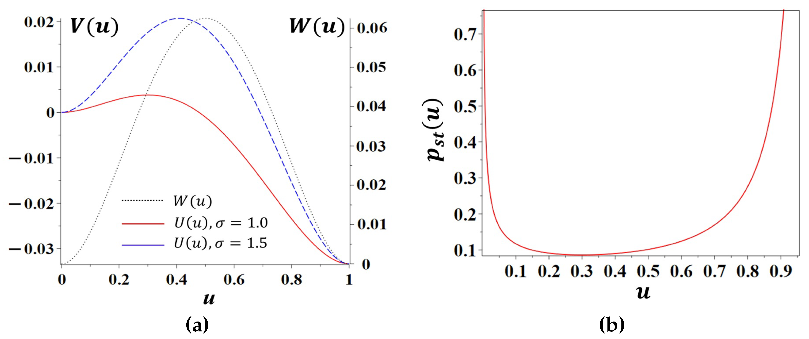
The associated Fokker–Planck equation for the density of on [22,25] admits a quasi-stationary solution whose shape is governed by the potential . In the regime where the noise-induced polarisation term dominates the deterministic bias r, develops two pronounced peaks near and and a pronounced minimum around . This structure is illustrated in Figure 1.
Figure 1 summarises the message of the local stochastic trust model. The polarisation potential and the effective potential landscape encoded in both single out the consensus configurations and as preferred states, while the internally polarised configuration is energetically and probabilistically disfavoured. Accordingly, a single hierarchical layer does not remain in a permanently split state: it tends to resolve internal polarisation by collapsing either into a stable trust phase () or into a stable distrust phase (), with noise-induced transitions between the two phases occurring on exponentially large time scales. These local bistable dynamics form the microscopic building blocks for the spatial domain formation and phase diagrams discussed in the subsequent subsections.
3.4. Fokker–Planck Equation and Stationary Distribution
The Itô form of the local stochastic dynamics at a single depth layer was obtained in Section 3.3 as
with drift and diffusion
as in (22)–(23). The evolution of the density of on is governed by the associated Fokker–Planck equation
supplemented by boundary conditions at and [22,25]. In the present setting both and vanish at the endpoints, so these boundaries are natural candidates for absorbing states. On very long time scales the true stationary distribution of (30) is therefore concentrated at and , corresponding to persistent distrust and persistent trust in the layer.
To understand how the robust phases and emerge and how they are separated by an unstable intermediate region, it is convenient to consider the stationary Fokker–Planck equation in the interior under the assumption of vanishing probability flux. This corresponds either to reflecting regularisations at the endpoints or to a quasi-stationary description conditioned on not having yet reached or . Denoting the stationary density by , stationarity and zero stationary flux give
Equation (33) is a first-order linear ODE that admits the standard explicit solution (see, e.g., [25])
where is a normalising constant whenever the integral converges.
Using (31), we have
The integral in (34) is elementary and can be evaluated in closed form. Since the explicit expression is somewhat cumbersome, we relegate its full derivation to Appendix A and only summarise the structure here. The stationary density on can be written as
where the effective potential is a smooth function incorporating both the noise-induced double-well structure and the deterministic logistic tilt. More precisely, contains a quartic contribution inherited from the potential in (29), together with additional logarithmic terms arising from the state-dependent diffusion coefficient .
In the regime where the noise-induced part of the drift dominates the deterministic term (for instance, when r is small compared to ), the leading contribution to is proportional to , so that
for some and a slowly varying prefactor that remains bounded and non-vanishing on . The qualitative shape of (36) is that of a double-peaked density: attains local maxima near and and a local minimum near . Thus, for a single depth layer, the noisy dynamics (18) admits two preferred configurations: one in which almost all agents persistently reject the assertion () and another in which almost all agents persistently accept it (), see Figure 1(b). The intermediate state , in which the layer is sharply divided, is statistically suppressed: it corresponds to the top of the effective potential barrier and plays the role of an unstable “saddle” between the two phases.
The parameters r and control the relative weight of these phases and the height of the barrier separating them. When is large and r is small, the noise-induced double well is nearly symmetric: the two peaks of have comparable height, and the layer has roughly symmetric chances to reside in a high-trust or high-distrust configuration, with rare noise-driven transitions between them, cf. Kramers-type transitions in double-well potentials [25,26]. When is not negligible, the deterministic logistic term tilts the effective potential in favour of trust: the well near becomes deeper and more probable, while the well near becomes shallower and less frequently visited. In this regime the layer still possesses two locally stable phases, but persistent trust dominates in the stationary statistics, and distrust appears mainly as a metastable configuration that can be overcome by fluctuations.
Thus, at the level of a single depth layer, the Fokker–Planck analysis confirms the picture suggested by the drift representation in Section 3.3: Stratonovich multiplicative noise with amplitude generates an effective double-well potential for the local trust variable u, with robust phases concentrated near and and a probabilistically suppressed intermediate state around .
While the stationary density in Figure 1 describes the long-run distribution over the trust level u, it is also instructive to visualise typical sample paths of the local process (30). The next figure shows numerically simulated trajectories for two noise intensities, illustrating how the same double-well landscape leads to very different escape times from the distrusting phase and different fluctuation patterns near full trust.
Figure 2 highlights the temporal manifestation of the two phases identified by the Fokker–Planck analysis. In the weak-noise regime, a layer may spend a very long time in the vicinity of before a sufficiently large fluctuation drives it across the potential barrier into the trusting phase , after which it undergoes only relatively small fluctuations around near-consensus. As increases, the effective barrier becomes easier to overcome, leading to much earlier entry into the trust well and stronger short-time variability near . In the hierarchical setting, such local episodes of slow escape from distrust and subsequent consolidation in trust form microscopic building blocks for the spatial patterns and domain dynamics discussed in the following subsections, where many layers interact along the depth axis of the hierarchy.
3.5. Field-Theoretic MSRJD Formulation of Noisy Trust Dynamics
We now return to the spatially extended setting and reintroduce the depth coordinate of the hierarchical DAG. The deterministic continuum limit of the network model is given by the degenerate logistic–diffusion equation (15), in which denotes the adoption probability (local social conformity) at depth x. To incorporate random fluctuations as discussed in Section 3.1–Section 3.4, we augment (15) by a multiplicative noise term with amplitude proportional to the local polarisation , interpreted in the Stratonovich sense in time. The resulting SPDE reads
where is the global noise intensity and is a Gaussian white noise with covariance .
As in the local analysis, it is convenient to convert (37) to Itô form before constructing the field-theoretic representation. The Stratonovich–Itô correction acts pointwise in x and produces the same noise-induced drift as in Section 3.3. Thus, in Itô form we obtain
with deterministic part
and noise-induced contribution
identical to the local term in (22). The function encodes, in the continuum setting, the effective double-well structure derived in Section 3.3 and is responsible for the emergence of robust local phases and at each depth.
To analyse rare events, nucleation of domains of trust and distrust, and large-scale fluctuations in the extended system, it is natural to use the Martin–Siggia–Rose–Janssen–De Dominicis (MSRJD) field-theoretic formalism [27,28,29,30,31]. In this approach one introduces an auxiliary response field and represents the statistics of (38) by a functional integral over paths weighted by an action . Formally, starting from (38), imposing the dynamics via a functional Dirac delta and integrating out the Gaussian noise yields the MSRJD action
where is given by (39) and is the observation horizon. The first term in (41) enforces the deterministic part of the SPDE through the response field , while the quadratic term in is the direct outcome of integrating over Gaussian noise with multiplicative amplitude .
Crucially, the deterministic functional in (41) contains exactly the same effective drift and noise-induced potential as those obtained from the Stratonovich–Itô conversion and the Fokker–Planck analysis in Section 3.3–Section 3.4. In particular, encodes the double-well structure associated with the quartic term , rendering and locally stable configurations of the belief field and an unstable saddle. The MSRJD formulation therefore does not change the underlying dynamics; it recasts the same noisy trust model in a form well suited for the systematic treatment of fluctuations and rare events.
Heuristically, functional variation of (41) with respect to reproduces the Itô SPDE (38), while variation with respect to u yields adjoint (instanton) equations describing the most probable paths associated with rare transitions between the trust and distrust phases. The Fokker–Planck equation (32) and its stationary solution (35) describe the same dynamics at the level of probability densities for at fixed depth. Thus the Itô Langevin formulation (38), the Fokker–Planck description, and the MSRJD action (41) are mutually consistent and complementary perspectives on the same stochastic model of trust formation in hierarchical societies.
From the modelling standpoint, the MSRJD framework is particularly useful in two contexts. First, it provides a natural language for analysing large deviations and nucleation events, in which a small domain of trust (or distrust) spontaneously appears within a background phase and either collapses or grows into a macroscopic region along the depth axis; in the weak-noise limit such events are governed by saddle points of (41). Second, the MSRJD action is the starting point for renormalisation-group analyses in higher-dimensional settings, where geometric fluctuations and long-range correlations may substantially modify the effective propagation and pinning of trust and distrust fronts. In the present work we use the MSRJD representation primarily as a conceptual bridge between the microscopic noise model and the emergent bistable potential structure; a more detailed study of instantons, nucleation rates and coarse-grained effective theories is deferred to future work and is briefly outlined in Appendix B.
3.6. Phase Selection and Social Interpretation of Trust/Distrust Phases
The analysis of the local SDE (18) and its Fokker–Planck equation (32) shows that multiplicative Stratonovich noise with amplitude generates an effective double-well structure for the belief variable at a fixed depth layer. Dynamically, the boundary states and act as two robust attractors of the stochastic dynamics (persistent distrust and persistent trust of the assertion within the layer), while the intermediate region near is unstable and statistically disfavoured. We now make this phase-selection picture explicit and connect it to the social interpretation of trust and distrust.
At the level of a single depth layer, the Itô SDE (30) describes a one-dimensional diffusion on with absorbing endpoints. Let be the first hitting time of ,
and let be the probability that a trajectory starting from is absorbed at rather than at ,
It is standard [25,32] that solves the boundary-value problem
with drift and diffusion coefficient given by (31). Although the explicit solution of (42) is cumbersome, its qualitative dependence on , r, and is clear. When the noise-induced double-well potential dominates (e.g. for small r and moderate ), is strongly curved: for slightly above the absorption probability at is close to one, whereas for slightly below it is close to zero, reflecting the unstable nature of the intermediate region and the strong attraction of the endpoints. When is sufficiently large compared to , the deterministic logistic term tilts the effective potential towards trust, and becomes biased in favour of , so that even initial conditions with may have a substantial chance to end in the trusting phase. Thus, for an individual layer, the noisy dynamics induces a probabilistic phase selection: starting from an internally mixed configuration, the layer ultimately consolidates either into distrust () or into trust (), with selection probabilities determined by and the parameters .
To illustrate these phase-selection probabilities quantitatively, we solve the boundary-value problem (42) numerically for a fixed noise level and two values of the amplification rate r. The resulting hitting probabilities for the trusting phase are shown in Figure 3.
Figure 3 confirms the strong tendency of the local process to end in the trusting phase. In the weakly biased case , the curve still exhibits a gradual increase as moves away from the fully distrusting state, reflecting some residual sensitivity to the initial trust level. When r is increased to , the graph is essentially saturated at except in an extremely small neighbourhood of , indicating that even layers starting with very low trust almost surely converge to . From a social perspective, this means that in a sufficiently favourable informational environment distrust becomes only metastable, while trust is the overwhelmingly preferred long-run outcome at the level of a single layer.
In the spatially extended model (38) along the depth axis x, this local bistability is coupled to degenerate diffusion via the term . For an initial profile that contains regions of intermediate values (polarised layers), the combined effect of spatial coupling, local double-well structure, and multiplicative noise produces a mosaic of trust and distrust along the hierarchy. In regions where is biased towards low values and the local tilt is weak, the dynamics drives the field towards the distrust phase ; in regions where is biased towards high values and/or is sufficiently positive, the field is driven towards the trust phase . At intermediate depths, where competing influences balance, the system develops narrow transition zones where passes sharply from values close to 0 to values close to 1. These zones act as domain walls or fronts separating stable trusting and distrusting regions, and their motion, pinning, and nucleation are governed by the interplay between degenerate diffusion, spatially varying , and noise level , in analogy with front dynamics and domain coarsening in bistable media [33,34].
To visualise these depth-wise domains of trust and distrust, Figure 4 shows a numerically computed long-time profile and the corresponding space–time evolution of for the degenerate logistic–diffusion equation (15) along the depth axis of the hierarchy.
In the top plot of Figure 4, the final profile is almost piecewise constant, with large intervals in which layers have converged either to or to . The narrow interfaces between these plateaus correspond to domain walls where the degenerate diffusion term and the local bias balance each other. The bottom plot shows that such profiles arise dynamically from an initially nearly homogeneous configuration: as time evolves, the local bistability of the effective potential amplifies small perturbations, nucleating domains of trust and distrust that then sharpen into plateaus and remain separated by relatively sharp fronts. In the full stochastic hierarchical model, these fronts become the natural mesoscopic objects whose motion and interactions encode large-scale reconfigurations of trust across the depth of the network.
The parameters of the model have a transparent interpretation in this phase-selection picture. The noise intensity plays the role of a “temperature of informational turbulence”: when is very small, transitions between phases are rare, domain walls are sharp and relatively immobile, and the pattern of trust and distrust is largely determined by the deterministic structure encoded in and . As increases, rare large fluctuations become more likely, enabling local patches of trust to nucleate within distrusting regions, and vice versa, and making domain walls more mobile and irregular. The effective amplification rate acts as a local “field” that biases the double–well potential towards trust or distrust at depth x: for the well at is deeper and more frequently occupied, while for negative the well at is favoured in the nearly deterministic regime. On intermediate time scales and for spatially varying , the hierarchy may therefore exhibit a transient polarised configuration in which some layers are locked in a trust phase and others in a distrust phase, separated by slowly evolving fronts.
To quantify the net outcome of this competition in the homogeneous case, we consider the long-time, depth-averaged trust level obtained from the SPDE (38) with constant coefficients. For each pair we simulate the hierarchical field over a long observation window, discard an initial transient, and compute the space–time average of along the depth axis. Figure 5 shows the resulting numerical phase diagram.
Figure 5 shows that, in this simple homogeneous setting, the distrust phase is only sustained when the amplification rate is negative and the informational turbulence is almost absent. As soon as is increased to moderate values, the diagram becomes essentially saturated in red: noise-assisted escapes from the low-trust well, combined with the logistic amplification towards , drive the hierarchy into a robust high-trust phase across the entire depth. Intermediate colours appear only in a thin low-noise band near , reflecting parameter combinations for which the system still spends a non-negligible fraction of time in both phases. Thus the phase diagram complements the local Kramers-type switching picture [26]: microscopic bistability at a single depth layer leads, at the macroscopic level, to either a global high-trust state or a narrow region of long-lived distrust, with only a very limited parameter window supporting persistent probabilistic coexistence of the two phases.
From a social perspective, the bistable structure of the local dynamics means that each depth layer is effectively faced with a communal choice of phase: over time, the layer either consolidates into a stable trusting disposition towards the assertion or into a stable distrusting disposition. The multiplicative noise with amplitude captures the empirical intuition that this choice is negotiated most intensely in internally divided layers, where disagreement and informational turbulence are greatest, while nearly unanimous layers are relatively inert to random perturbations. In contrast to the purely deterministic logistic model, which typically leads to a unique homogeneous attractor, the stochastic model naturally accommodates stable polarisation and metastable transitions between trust and distrust. It thereby provides a probabilistic theory of trust formation over a hierarchical backbone: long-lived trust and distrust emerge as stochastic phases of the belief field , shaped jointly by the underlying network structure and by the intensity and structure of random informational shocks.
4. Discussion
The present framework connects naturally to classic sociological theories of trust while recasting trust as a stochastic phase of a belief field on a hierarchical network. In Luhmann’s systems perspective, trust functions as a device for reducing social complexity, enabling action under uncertainty by bracketing possible contingencies [5]. In our setting, this reduction appears when agents compress rich social information into a binary adoption decision for a single assertion. Yet, unlike static views of trust as a background condition, the binary state in our model is an emergent, noise-driven configuration that can switch in time. Coleman’s conception of trust as a form of social capital embedded in structured networks [6] is reflected in the explicit role of network position and hierarchical depth: influence weights and depth-dependent amplification determine how local trust or distrust is reinforced and propagated. Gambetta’s micro-level interpretation of trust as an expectation of cooperative or reliable behaviour under uncertainty [7] is captured by the probabilistic interpretation of as a local adoption probability. Taken together, these perspectives are complemented rather than replaced: we retain the ideas of complexity reduction and network-embedded expectations, but formalise trust as a bistable probability field on a directed hierarchical graph, shaped jointly by structured influence and stochastic fluctuations.
This simplified paradigm also aligns with, and deliberately abstracts from, multidimensional models of interpersonal and organisational trust. Mayer, Davis, and Schoorman conceptualise trustworthiness along several distinct dimensions (ability, benevolence, integrity) that jointly determine whether a trustee is judged trustworthy [8]. Our model effectively collapses these facets into a single outcome variable: an agent either accepts or rejects the assertion, which can be read as a coarse-grained indicator of overall trust in the source or content. The simplicity of a scalar u makes the stochastic analysis tractable, but it suppresses the reasons why trust is granted or withheld. A natural extension is to replace u by a low-dimensional trust vector, with components corresponding, for example, to credibility of content, perceived benevolence of the source, or institutional reliability. The present scalar model can then be viewed as the first component of a richer trust field, illustrating how network structure and noise alone already generate persistent trust/distrust phases even before these additional dimensions are resolved.
Beyond sociology, our results resonate with pattern formation and phase separation in reaction–diffusion systems and statistical physics. The continuum limit produces a degenerate logistic–diffusion equation whose nonlinear reaction term and state-dependent diffusion naturally permit domain structures, in contrast to purely diffusive or linear consensus models. In classical reaction–diffusion theory, homogeneous equilibria may destabilise and give rise to spatially heterogeneous patterns through diffusion-driven instabilities [19]. In our hierarchical setting, the coupling between depth layers, encoded via the effective diffusion coefficient , and the local double-well potential induced by multiplicative Stratonovich noise, leads to stable domains of high trust and high distrust separated by relatively sharp fronts, reminiscent of phase separation rather than smooth averaging. This contrasts with linear averaging models of opinion dynamics, such as DeGroot’s model and related consensus schemes, where opinion mass is conserved and trajectories generically converge to a single, typically homogeneous, attractor [9]. Here no such conservation law holds: the depth-integrated “mass of conviction” is not preserved, and the system admits multiple long-lived configurations corresponding to coexisting trust and distrust domains. The analogy with spin systems and bistable media is immediate: the field u plays the role of an order parameter, with and behaving like competing phases whose domains coarsen, drift, and pin under the combined influence of network structure and noise, akin to domain formation and coarsening in non-conserved order-parameter dynamics [34]. This places the model alongside network-based opinion and polarisation models that explicitly admit stable clustering and echo chambers rather than inevitable consensus [11].
At the same time, the modelling assumptions entail important limitations. First, the trust state is binary: each agent either adopts or rejects the assertion, so intermediate or ambivalent attitudes are not represented. This is appropriate for settings where the relevant behaviour is indeed dichotomous (accept/deny, share/block) but it underrepresents gradations of confidence and nuanced positions. Second, the hierarchical directed acyclic graph is static; there is no adaptation of the network in response to trust outcomes. In empirical settings, trust and structure co-evolve: connections may weaken or dissolve when trust erodes, or new links may form towards highly trusted sources. Third, only a single assertion is considered; the model does not accommodate competing narratives or cross-topic interactions, even though real agents continuously arbitrate between multiple, sometimes mutually exclusive, claims. Fourth, randomness is represented by Gaussian white noise without memory. This captures diffuse micro-level uncertainty but not rare, heavy-tailed shocks such as scandals or crises that can reconfigure trust on short time scales. Finally, there is no endogenous feedback from the trust field back to the structural parameters and : local levels of trust do not modify influence strengths or the effective amplification rate. These simplifications mean that the present framework should be interpreted as an analytically tractable baseline rather than a full account of trust in complex societies.
Several directions suggest themselves for future work. A first step is to promote u from a scalar to a vector-valued field, with components encoding different aspects of trustworthiness or trust in multiple sources and topics, which would align more closely with multidimensional theories of trust and allow for cross-couplings between dimensions. Second, the hierarchical structure could be generalised to multilayer or multiplex networks, with distinct layers representing, for instance, face-to-face interactions, institutional communication, and online platforms, and with interlayer couplings mediating cross-channel reinforcement or interference. Third, the topology and influence weights could be allowed to adapt in time in response to local trust levels, introducing a coevolution of trust and network structure in which trusted nodes accumulate influence and distrusted ones lose it. Finally, parameters such as the amplification rate r, noise intensity , and effective diffusion D could be calibrated to empirical data, for example from panel surveys on institutional trust or observed cascades of belief on online platforms, to test whether the phase diagrams and domain structures predicted by the model correspond to measurable patterns of trust and distrust in real hierarchical organisations.
In summary, by embedding trust dynamics in a probabilistic network model and its continuum limit, and by explicitly incorporating multiplicative noise, we have shown how stable trust and distrust phases can emerge as stochastic equilibria of a belief field on a hierarchical backbone. This view is consistent with, and gives a quantitative counterpart to, classical sociological accounts that emphasise complexity reduction, network-embedded expectations, and the structural role of trust [5,6,7], while also drawing on analogies with bistable media and pattern formation. At the same time, it opens a pathway towards more elaborate models in which the richness of empirical trust phenomena—their multidimensionality, multi-channel propagation, and coevolution with social structure—can be progressively incorporated into a unified stochastic field-theoretic description.
5. Conclusion
Recent empirical debates about a “crisis of trust” motivated this work: survey evidence points to long-lived islands of high trust and deep distrust in institutions and information systems, as well as abrupt shifts triggered by scandals or shocks. Against this backdrop we asked three related questions: why communities that appear similar in their informational environment can stabilise in very different states (persistent trust versus persistent distrust), why hierarchically organised systems tend to develop robust pockets of trust and distrust along the same organisational backbone, and why changes in trust often occur in sudden jumps rather than as slow, incremental adjustments. Within our framework, these phenomena arise from the combination of hierarchical geometry, a non-conservative degenerate logistic–diffusion mechanism for belief propagation, and noise-induced bistability of the local trust variable, which together generate coexisting trust and distrust phases and rare stochastic transitions between them.
At the level of a single depth layer, the stochastic dynamics already admits two locally stable phases, and , and the eventual state is not predetermined but selected probabilistically as a function of the initial condition and the parameters . In the full hierarchical setting, differences in the initial belief configuration , in the depth-dependent amplification profile (reflecting distinct institutional or contextual environments), and in the hierarchical structure encoded by the effective influence kernel S and diffusion coefficient can therefore lead formally similar communities, exposed to comparable information, to lock into different phases: one may converge to a predominantly trusting regime, while another of similar size and average conditions settles into persistent distrust. The model thus provides a precise mechanism for diverging trust trajectories under ostensibly comparable informational conditions: modest variations in structure, initialisation, and noise level translate into systematic differences in the probabilistic selection between trust and distrust phases.
Along the depth axis of the hierarchy, the continuum limit leads to a non-conservative degenerate logistic–diffusion equation of the form
for the adoption probability . Combined with the local bistability of the stochastic layer dynamics (two stable phases near and ), the degeneracy of diffusion (diffusive coupling effectively switches off in saturated regions with or ) and spatial heterogeneity of generates extended domains of trust and distrust along the hierarchical backbone, separated by relatively narrow fronts. Socially, these domains correspond to pockets of persistent trust or persistent distrust in the same institution or message within a single hierarchical system (such as a state, corporation, or expert community), while the fronts mark sharp boundaries between groups that interpret the same actor or narrative in fundamentally different ways. Because diffusion is weak in saturated layers and motion of the fronts requires overcoming local potential barriers through rare fluctuations, such trust and distrust pockets are structurally robust and difficult to reconfigure by incremental signals alone.
At the local level, the Stratonovich–Itô analysis shows that the multiplicative noise generates an effective double-well potential for u, so that the belief variable fluctuates around one of two wells (trust or distrust) and can undergo noise-induced transitions across the intervening barrier. For fixed parameters the system typically spends very long periods in one phase, but with small probability a fluctuation is large enough to push a layer, or an extended domain, from the distrust well to the trust well, or vice versa. In social terms, scandals, crises, and informational shocks are naturally interpreted as such atypical excursions: they trigger abrupt regime shifts in trust that are followed by equally long plateaux in the new phase, thereby producing step-like, yet persistent, changes in collective attitudes. The Fokker–Planck description and the MSRJD field-theoretic formulation provide a large-deviation framework for quantifying these rare transitions between trust and distrust basins, even though detailed asymptotic calculations of switching rates are left for future work.
Taken together, the results address the three motivating questions from Section 1. First, differences in long-run trust or distrust across communities exposed to seemingly similar information arise from probabilistic phase selection in a locally bistable dynamics, modulated by heterogeneous hierarchical structure and amplification profiles. Second, stable pockets of trust and distrust within a single hierarchy emerge as depth-wise domains of the belief field, supported by the combination of local bistability and degenerate diffusion that switches off in saturated layers. Third, abrupt changes in trust correspond to noise-induced transitions across barriers of the effective potential, producing rare but persistent regime shifts between trust and distrust phases. In this sense, the model frames trust as a noise-sustained phase of a belief field on a hierarchical network rather than a fixed attribute of actors, complementing rather than replacing classical sociological and organisational accounts by providing an explicit stochastic, depth-resolved mechanism for the emergence, coexistence, and sudden reconfiguration of trust and distrust in complex social systems.
The present framework remains deliberately stylised: it focuses on a single assertion with a binary trust variable , evolves on a fixed hierarchical network, and is driven by Gaussian, memoryless noise. These simplifications, discussed in more detail in Section 4, point directly to future work on multidimensional trust fields (e.g. trust in different attributes or sources), adaptive and multilayer network structures, and empirical calibration of parameters such as , and from survey or panel data on institutional trust. We expect that such extensions will make it possible to connect the model more tightly to concrete applications, from organisational communication to online information ecosystems, while preserving the core mechanism of stochastic trust phases on hierarchical backbones. More broadly, the framework offers a compact language in which crises of trust, persistent islands of trust and distrust, and their sensitivity to political, institutional, or informational interventions can be formulated and, in the longer run, analysed quantitatively.
Funding
This research received no external funding.
Institutional Review Board Statement
Not applicable.
Data Availability Statement
The original contributions presented in this study are included in the article. Further inquiries can be directed to the corresponding author.
Acknowledgments
The authors are grateful to their institutions for the administrative and technical support.
Conflicts of Interest
The author declares no conflict of interest.
Appendix A. Stationary Fokker–Planck Solution for a Single Depth Layer
We briefly derive the stationary solution of the Fokker–Planck equation associated with the local Itô dynamics (30) and examine its small- and large-noise limits. Recall the scalar SDE on ,
with
and the corresponding Fokker–Planck equation for the density on ,
On the open interval we consider stationary solutions with vanishing probability flux (detailed balance). Writing for a stationary density, the probability flux
vanishes if and only if
For a one-dimensional diffusion, this first-order equation has the standard solution
where C is chosen (if possible) to normalise .
Substituting (A2) into (A5) yields and
so the integral is elementary. Up to an overall multiplicative constant,
For generic and this formal density is not integrable on because of power-law divergences at and . This is consistent with the fact that the SDE with absorbing boundaries at and has a true stationary measure supported on the set , namely a convex combination of and . Nevertheless, (A7) is useful as a quasi-stationary density describing the relative likelihood of interior values before absorption at the endpoints.
It is convenient to rewrite (A7) in exponential form
with effective potential
The logarithmic terms originate from the state-dependent diffusion and dominate the behaviour of near the boundaries, where vanishes. Away from and , this structure is consistent with the drift-based potential picture developed in Section 3.3, where the Stratonovich multiplicative noise generates an effective double-well contribution proportional to in the deterministic part of the dynamics.
The explicit expression (A7) allows a simple characterisation of the regimes and . When one has , and
so mass concentrates near . This reflects the deterministic logistic drift, which drives almost all trajectories to the trusting phase , and the true stationary measure converges to .
In the opposite regime , the ratio and
up to slowly varying corrections. The interior quasi-stationary density is then symmetrically peaked near both boundaries, corresponding to frequent noise-driven passages between and and a negligible deterministic tilt. In both limits remains non-normalisable on , in agreement with the presence of absorbing boundaries and a true stationary measure supported on . The explicit interior solution nevertheless confirms the qualitative picture from the main text: intermediate values are strongly suppressed, while the two extremal phases (persistent distrust) and (persistent trust) act as robust attractors of the stochastic dynamics for a single hierarchical layer.
Appendix B. MSRJD Functional for the Noisy Hierarchical Model
In this appendix we sketch the derivation of the Martin–Siggia–Rose–Janssen–De Dominicis (MSRJD) functional for the noisy hierarchical trust model, starting from the Itô SPDE that already contains the noise-induced drift identified at the single-layer level.
The depth-resolved belief field on evolves according to
with deterministic part
and noise-induced drift
as in (40). The Gaussian space–time white noise has zero mean and covariance
and formal measure on
The probability weight of a trajectory can be written as an average over noise realisations, constrained by the SPDE (A12),
where we abbreviate , , and denotes a functional Dirac delta. Introducing a real response field , we represent the delta functional as
Substituting (A16) and (A18) into (A17) yields
The dependence on in the exponent of (A19) is
which can be completed to a square pointwise:
Inserting (A21) into (A19) and integrating over (which contributes only an overall normalisation), we obtain
with MSRJD action
Up to notation, this coincides with the functional introduced in Section 3.5. The first term enforces the deterministic drift—including the noise-induced double-well structure identified in the Stratonovich analysis—while the quadratic term in encodes the multiplicative noise with amplitude .
In a weak-noise (saddle-point) approximation, typical rare-event paths are obtained from the stationarity conditions of . Variation with respect to gives
so that
The complementary Euler–Lagrange equation yields the adjoint (“instanton”) dynamics for , involving the operator and derivatives of both and ; its explicit form is standard and omitted here. The connection to the original SPDE (A12) follows from the shift used in completing the square: along an optimal fluctuation one effectively has , and substituting this into (A12) reproduces (A25).
Thus the MSRJD functional (A23) provides a compact field-theoretic representation of the noisy hierarchical trust dynamics, consistent with both the Itô SPDE description and the single-layer Fokker–Planck analysis in Appendix A. It gives a natural starting point for the study of fluctuation-induced nucleation of trust/distrust domains and for large-deviation or renormalisation-group analyses of the stochastic hierarchical model.
Appendix C. Abbreviations
The following abbreviations are used in this manuscript:
| BVP | boundary value problem |
| DAG | directed acyclic graph |
| MSRJD | Martin–Siggia–Rose–Janssen–De Dominicis |
| ODE | ordinary differential equation |
| SDE | stochastic differential equation |
| SPDE | stochastic partial differential equation |
References
- Edelman. 2024 Edelman Trust Barometer: Innovation in Peril; Edelman, 2024. [Google Scholar]
- Pew Research Center. News consumption and trust in the digital age. Pew Research Center Report, 2024.
- Pew Research Center. Public trust in scientists and views on science. Pew Research Center Report, 2024.
- Gillespie, N.; Lockey, S.; Ward, T.; Macdade, A.; Hassed, G. Trust, Attitudes and Use of Artificial Intelligence: A Global Study 2025; University of Melbourne and KPMG International, 2025. [Google Scholar]
- Luhmann, N. Trust and Power; Wiley: Chichester, 1979. [Google Scholar]
- Coleman, J.S. Foundations of Social Theory; Harvard University Press: Cambridge, MA, 1990. [Google Scholar]
- Gambetta, D.; Ed. Trust: Making and Breaking Cooperative Relations; Basil Blackwell: Oxford, 1988. [Google Scholar]
- Mayer, R.C.; Davis, J.H.; Schoorman, F.D. An integrative model of organizational trust. Academy of Management Review 1995, 20, 709–734. [Google Scholar] [CrossRef]
- DeGroot, M.H. Reaching a consensus. Journal of the American Statistical Association 1974, 69, 118–121. [Google Scholar] [CrossRef]
- Easley, D.; Kleinberg, J. Networks, Crowds, and Markets: Reasoning about a Highly Connected World; Cambridge University Press: Cambridge, 2010. [Google Scholar]
- Castellano, C.; Fortunato, S.; Loreto, V. Statistical physics of social dynamics. Reviews of Modern Physics 2009, 81, 591–646. [Google Scholar] [CrossRef]
- Hegselmann, R.; Krause, U. Opinion dynamics and bounded confidence: Models, analysis and simulation. Journal of Artificial Societies and Social Simulation 2002, 5, 2. [Google Scholar]
- Volchenkov, D.; Putkaradze, V. Mathematical Theory of Social Conformity I: Belief Dynamics, Propaganda Limits, and Learning Times in Networked Societies. Mathematics 2025, 13, 1625. [Google Scholar] [CrossRef]
- Volchenkov, D. Mathematical Theory of Social Conformity II: Geometric Pinning, Curvature–Induced Quenching, and Curvature–Targeted Control in Anisotropic Logistic Diffusion. Dynamics 2025, 5, 27. [Google Scholar] [CrossRef]
- Medvedev, G.S. The nonlinear heat equation on dense graphs and graph limits. SIAM Journal on Mathematical Analysis 2014, 46, 2743–2766. [Google Scholar] [CrossRef]
- Lovász, L. Large Networks and Graph Limits; American Mathematical Society: Providence, RI, 2012. [Google Scholar]
- Fisher, R.A. The wave of advance of advantageous genes. Annals of Eugenics 1937, 7, 355–369. [Google Scholar] [CrossRef]
- Kolmogorov, A.N.; Petrovskii, I.G.; Piskunov, N.S. A study of the equation of diffusion with increase in the quantity of matter, and its application to a biological problem. Bulletin of Moscow State University, Series A: Mathematics and Mechanics 1937, 1, 1–25. [Google Scholar]
- Murray, J.D. Mathematical Biology I: An Introduction, 3rd ed.; Springer: New York, 2002. [Google Scholar]
- Vázquez, J.L. The Porous Medium Equation: Mathematical Theory; Oxford University Press: Oxford, 2007. [Google Scholar]
- Horsthemke, W.; Lefever, R. Noise-Induced Transitions: Theory and Applications in Physics, Chemistry, and Biology; Springer: Berlin, 1984. [Google Scholar]
- Gardiner, C.W. Handbook of Stochastic Methods for Physics, Chemistry and the Natural Sciences, 3rd ed.; Springer: Berlin, 2004. [Google Scholar]
- van Kampen, N.G. Stochastic Processes in Physics and Chemistry, 3rd ed.; North-Holland: Amsterdam, 2007. [Google Scholar]
- Arnold, L. Random Dynamical Systems; Springer: Berlin, 1998. [Google Scholar]
- Risken, H. The Fokker–Planck Equation: Methods of Solution and Applications, 2nd ed.; Springer: Berlin, 1996. [Google Scholar]
- Freidlin, M.I.; Wentzell, A.D. Random Perturbations of Dynamical Systems, 3rd ed.; Springer: Heidelberg, 2012. [Google Scholar]
- Martin, P.C.; Siggia, E.D.; Rose, H.A. Statistical dynamics of classical systems. Physical Review A 1973, 8, 423–437. [Google Scholar] [CrossRef]
- Janssen, H.K. On a Lagrangean for classical field dynamics and renormalization group calculations of dynamical critical properties. Zeitschrift für Physik B 1976, 23, 377–380. [Google Scholar] [CrossRef]
- De Dominicis, C. Technics of field renormalization and dynamics of critical phenomena. Journal de Physique Colloques 1976, 37, C1-247–C1-253. [Google Scholar]
- Täuber, U.C. Critical Dynamics: A Field Theory Approach to Equilibrium and Non-Equilibrium Scaling Behavior; Cambridge University Press: Cambridge, 2014. [Google Scholar]
- Kamenev, A. Field Theory of Non-Equilibrium Systems; Cambridge University Press: Cambridge, 2011. [Google Scholar]
- Redner, S. A Guide to First-Passage Processes; Cambridge University Press: Cambridge, 2001. [Google Scholar]
- Fife, P.C. Mathematical Aspects of Reacting and Diffusing Systems; Springer: Berlin, 1979. [Google Scholar]
- Bray, A.J. Theory of phase-ordering kinetics. Advances in Physics 1994, 43, 357–459. [Google Scholar] [CrossRef]
Figure 1.
Local potential landscape and quasi-stationary density (numerical). (a) An effective double-well profile (left vertical axis), representing a monotone rescaling of the potential , plotted together with the polarisation potential (right vertical axis). Both profiles single out the consensus states and as preferred and penalise the internally polarised state . (b) A corresponding quasi-stationary density with two peaks near and and a minimum around , illustrating the coexistence of persistent distrust and trust phases at the level of a single depth layer.
| (a) | (b) |
Figure 2.
Sample paths of the local Itô diffusion (30) for two values of the noise intensity (numerical simulation). Both trajectories start near the distrusting well . For moderate noise (blue dashed curve, ) the process wanders for a long time in the low- and intermediate-trust region before eventually reaching the trusting phase , where it then fluctuates around near-consensus. For stronger noise (red solid curve, ) the process reaches the trusting phase much earlier and then remains close to over the observation window.
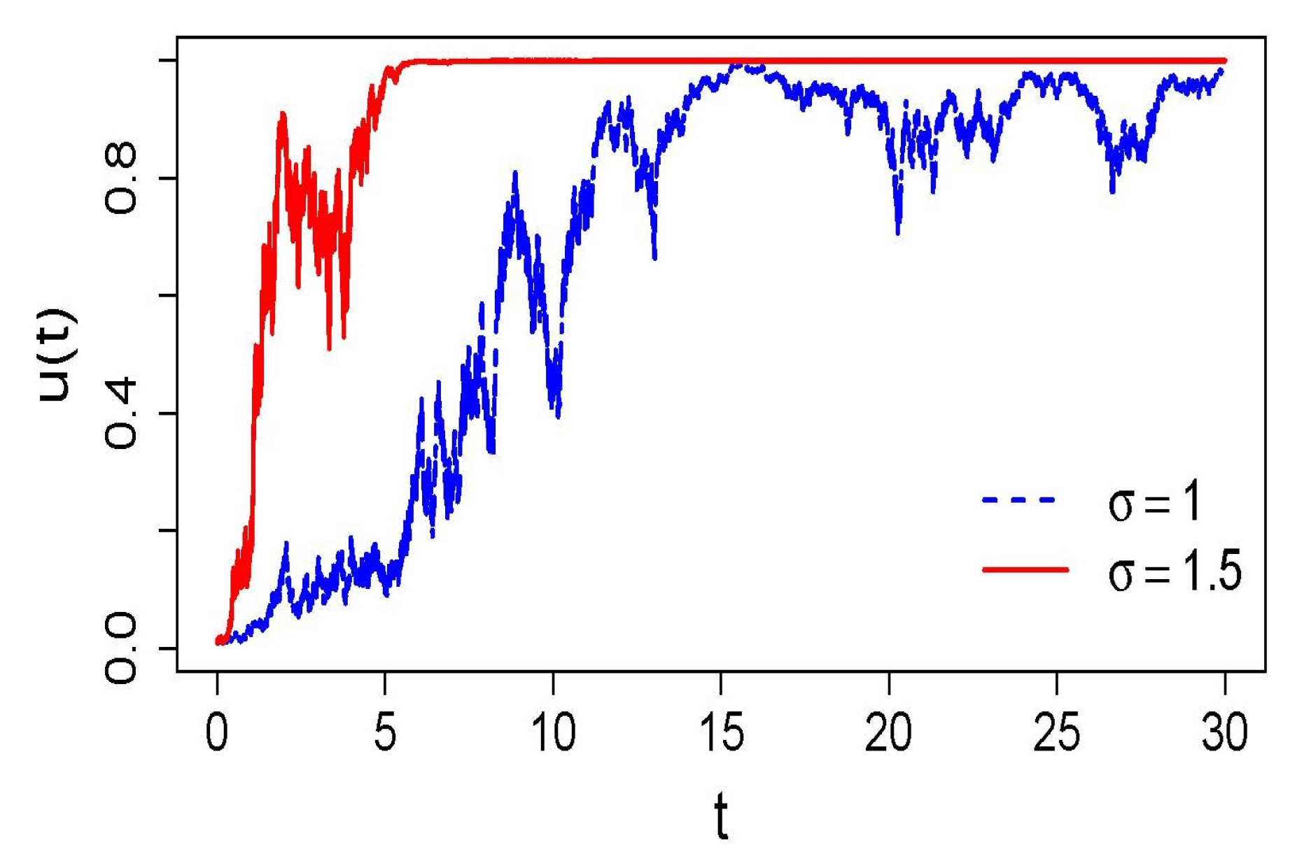
Figure 3.
Hitting probability of the trusting phase for the local diffusion (30). The plot shows the solution of the boundary-value problem (42) for fixed noise intensity and two amplification rates: a weak bias (blue) and a stronger bias (red). For almost all initial conditions the process is absorbed in the trusting phase with very high probability; increasing r compresses the residual basin of the distrusting phase into a small neighbourhood of .
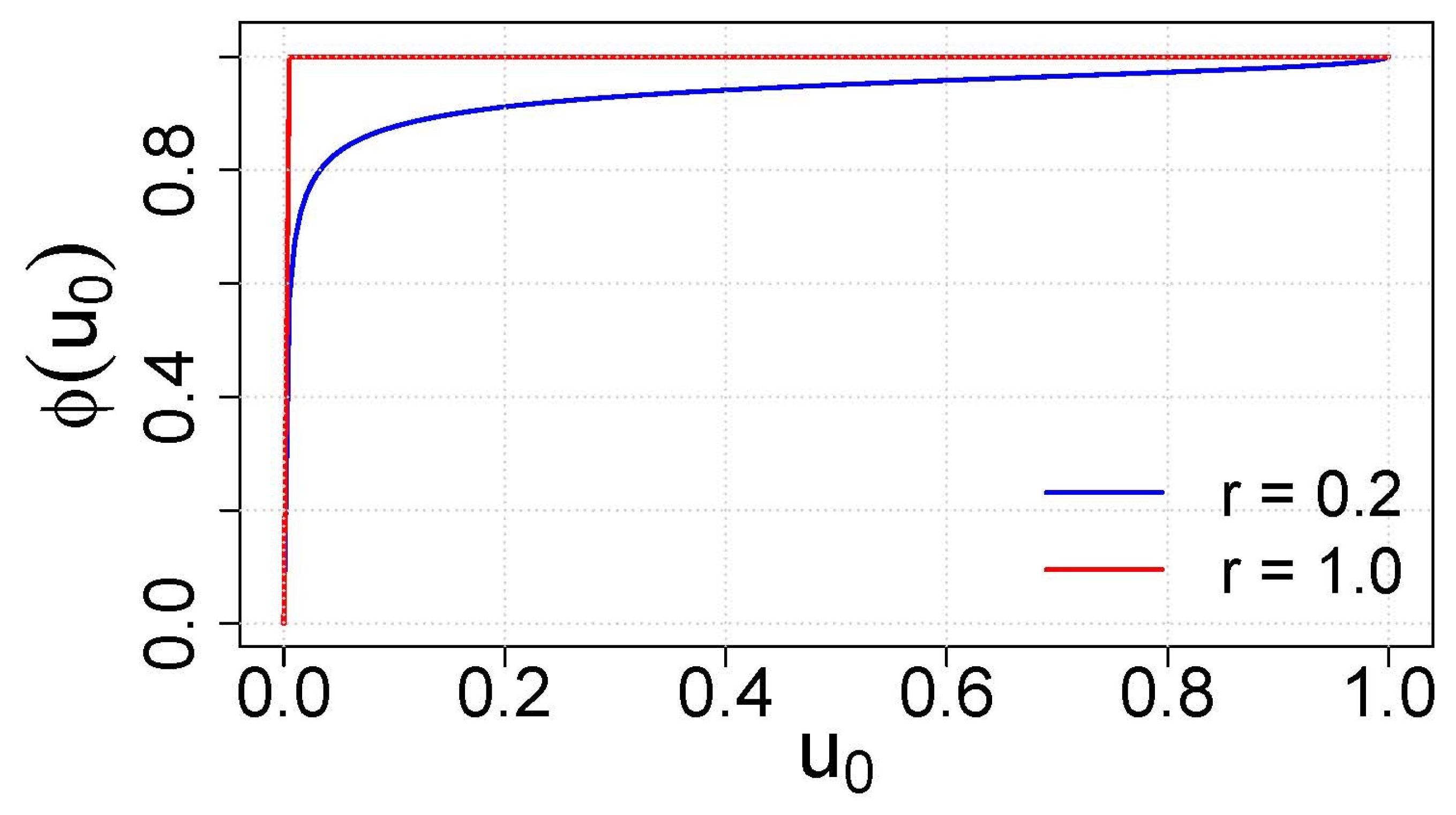
Figure 4.
Trust/distrust domains along the depth of the hierarchy (numerical simulation). Top: final profile exhibiting two extended regions with (distrust) and (trust), separated by narrow transition layers. Bottom: space–time heatmap of in a symmetric case, illustrating how an initially weakly structured state evolves into a persistent mosaic of trusting and distrusting depth layers.
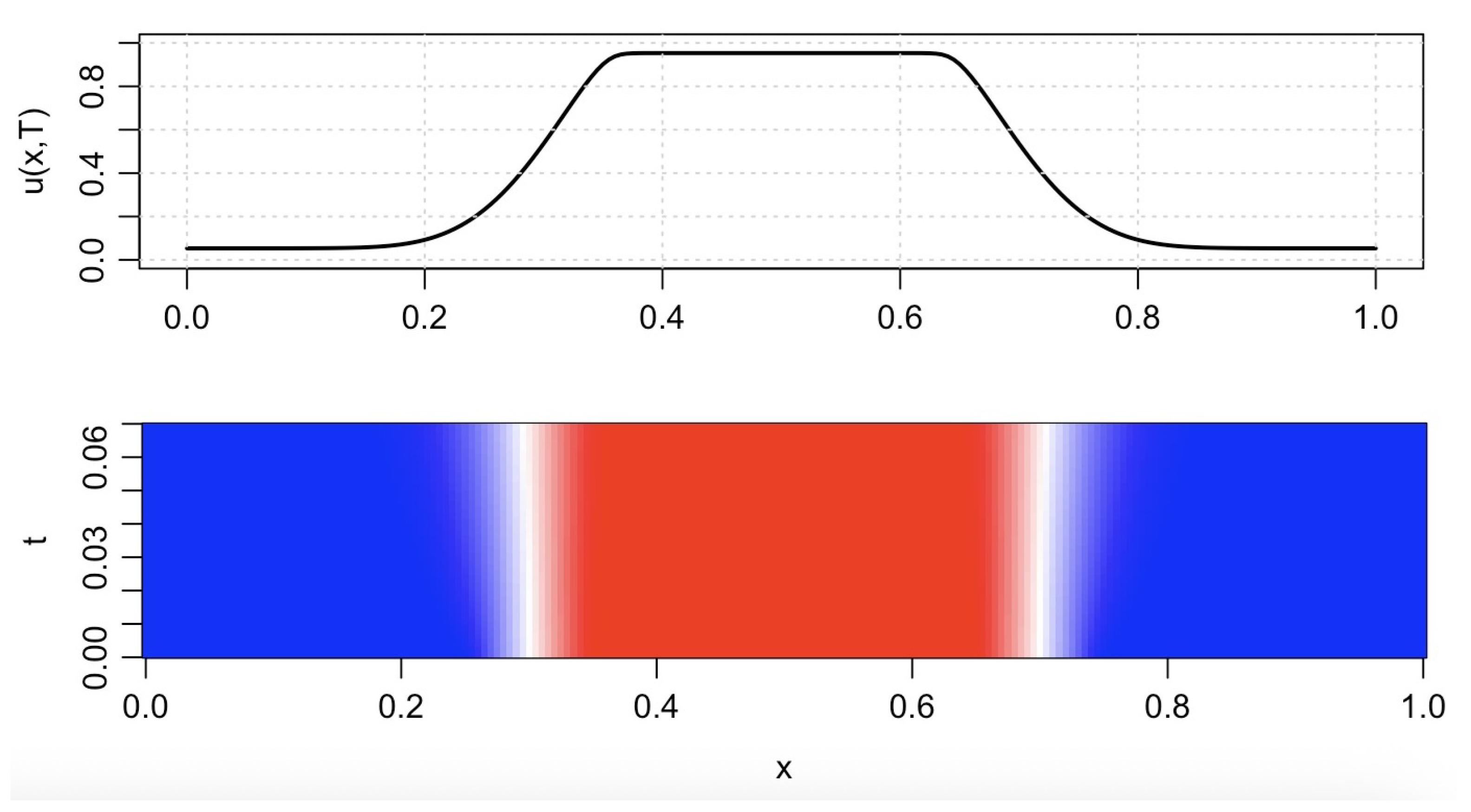
Figure 5.
Phase diagram in the plane (numerical simulation). Colour encodes the long-time, depth-averaged trust level obtained from simulations of SPDE (38) with constant D, r and . Blue corresponds to predominantly distrusting configurations (), red to predominantly trusting configurations (), and intermediate shades indicate mixed states with substantial time spent in both phases. For the parameter range shown, a low-trust regime is confined to a narrow band of very small noise intensities and moderately negative r, while almost all other parameter combinations yield a trust-dominated state.
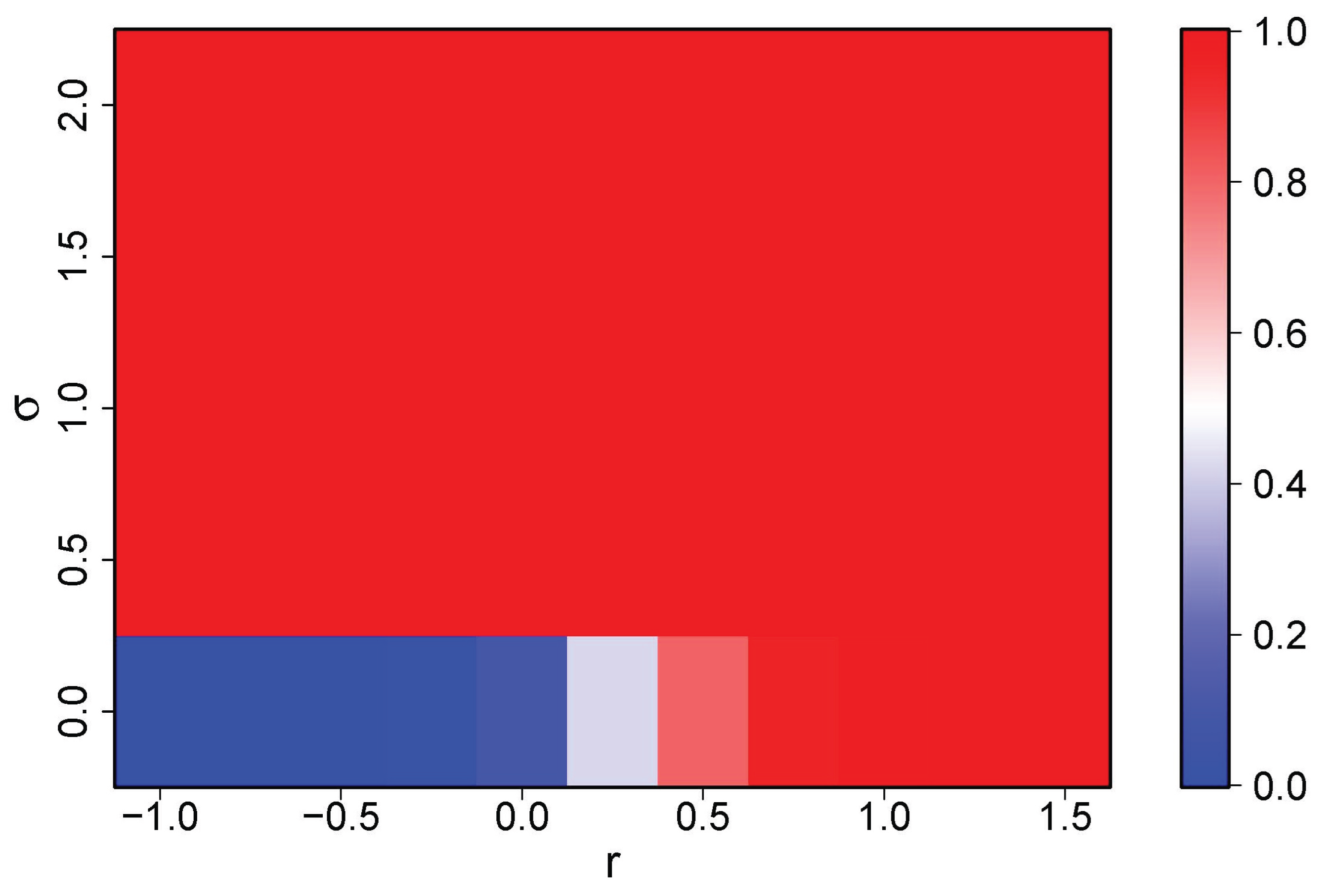
Disclaimer/Publisher’s Note: The statements, opinions and data contained in all publications are solely those of the individual author(s) and contributor(s) and not of MDPI and/or the editor(s). MDPI and/or the editor(s) disclaim responsibility for any injury to people or property resulting from any ideas, methods, instructions or products referred to in the content. |
© 2025 by the authors. Licensee MDPI, Basel, Switzerland. This article is an open access article distributed under the terms and conditions of the Creative Commons Attribution (CC BY) license (http://creativecommons.org/licenses/by/4.0/).
Copyright: This open access article is published under a Creative Commons CC BY 4.0 license, which permit the free download, distribution, and reuse, provided that the author and preprint are cited in any reuse.


