
Submitted:
26 November 2025
Posted:
27 November 2025
You are already at the latest version
Abstract
Fractional transforms have emerged as powerful analytical tools that bridge the time, frequency, and scale domains by introducing a fractional-order parameter into the kernel of classical transforms. This survey provides an overview of the mathematical foundations and distributional frameworks of several key fractional transforms, with emphasis on their formulation within appropriate spaces of generalized functions. Particular attention is devoted to the quasiasymptotic behavior of distributions in relation to the asymptotic properties of their corresponding fractional transforms. Moreover, we apply the considered transforms to the same sample signal and perform a comparative analysis.
Keywords:
quasiasymptic behaviour
; distributions
; fractional integral transforms
1. Introduction
To convert a signal into a form more suitable for analysis and processing, the term transformation is often employed. In many cases, the original signal representation is inconvenient to work with; hence signal transforms are applied to obtain representations that are easier to handle. Among the most commonly used are the Fourier transform (FT) [1,2,3], the Fourier cosine transform (FCT) and the Fourier sine transform (FST), the short-time Fourier transform (STFT) [4], the wavelet transform (WT) [5,6], the Stockwell transform (ST) [7] and the Hankel transform (HT) [8].
Over the past two decades, fractional transforms have become increasingly important in diverse fields such as signal and image processing, optics, geo-informatics, radar and communication systems, as well as biomedical applications (see Section 11). The basic idea behind fractional transforms is to replace the conventional kernel of the transform by a fractional kernel, thereby introducing an extra continuous parameter that permits interpolation between domains (for example between time and frequency). This extra degree of freedom often enables improved representations, enhanced adaptability or improved resolution in joint domains.
The archetype of these fractional transforms is the fractional Fourier transform (FRFT). Historically, although the idea of fractional powers of the Fourier operator can be traced back to early work by Norbert Wiener (1929) and Condon (1937) in the context of phase-space or harmonic oscillator Green’s functions, the formalisation in the signal-processing/ transform-theory community is commonly credited to V. Namias in 1980, who proposed the operator approach for the fractional Fourier transform in the context of quadratic Hamiltonians. [9]. The FRFT is an extension of the classical Fourier transform (FT). As explained in Ozaktas et al. [10] , “the -th order fractional Fourier transform is the -th power of the Fourier transform operator” and the parameter effectively enables rotation by an arbitrary angle in the time–frequency plane.
Because the FRFT generalises and enriches the classical transform domain, it opens the way for a family of fractional versions of many other classical transforms. The survey of such fractional forms is timely because they promise advanced flexibility in representing non-stationary, multi-scale and multi-domain signals, but the literature is fragmented and each fractional version has its own nuances (kernel definitions, additivity properties, inversion, interpretation). In particular, the fractionalisation of each classical transform often aims to preserve key structural properties (such as index-additivity, unitarity, invertibility, resolution trade-offs) while adding the continuous parameter that allows “rotation” or interpolation between domains.
The classical STFT replaces the global Fourier kernel by a time-windowed kernel, enabling time–frequency localisation. However, it remains anchored to the standard Fourier domain. One limitation is that for certain types of signals (such as chirps, or signals with components that rotate in the time–frequency plane), the fixed rotation may not be optimal. The short-time fractional Fourier transform (STFRFT) was proposed in [11] to overcome the limitation of the FRFT in identifying frequency components in the fractional Fourier domain. The STFRFT retains essential properties of the STFT (windowing, invertibility, time–fractional-frequency analysis) while enabling a fractional rotation in the time/frequency plane.
While the FRFT generalises the FT, the fractional Fourier cosine (FRFCT) and sine (FRFST) transforms have been introduced more recently: in [12] the real and imaginary parts of the FRFT kernel were used to define FRFCT and FRFST, though those initial definitions lacked additivity (index-sum property) and thus could not strictly be considered “true fractional” extensions. Later work (e.g., [13], and also [14,15]) proposed additive versions that maintain analogous relationships with the FRFT.
The fractional wavelet transform (FRWT) is an extension of the classical WT that incorporates the FRFT into its kernel. By introducing a fractional-order parameter, the FRWT allows the localization of a signal to be adjusted continuously between the time and frequency domains, thereby providing an additional degree of flexibility in time–frequency analysis. This adaptability enables improved representation of non-stationary and chirp-like signals, while preserving the multi-resolution nature of the standard WT. The FRWT has proven particularly effective in reducing reconstruction error and improving energy concentration in applications involving denoising, compression, and signal characterization.
The classical Stockwell transform blends elements of STFT and WT, providing time-frequency localisation with a frequency-dependent window. The fractional Stockwell transform (FRST) (first introduced in [16] for seismic data analysis) replaces the Fourier kernel with a fractional one, thus adding a fractional rotation parameter and offering enhanced time–fractional-frequency resolution compared to the classical ST. The FRST provides enhanced analysis capabilities for non-stationary signals, offering a flexible framework that bridges the ST, STFT, and FRFT domains. Owing to its improved resolution and adaptability, the FRST has found significant applications in geophysical data analysis, seismic signal interpretation, and other fields requiring high-precision time–frequency characterization.
The HT plays a key role in radially-symmetric or cylindrical problems (for example in optics, wave propagation, scattering). The fractional Hankel transform (FRHT) replaces the Bessel-function kernel of the HT by a fractional-order kernel (or via eigenfunction expansions) to introduce a fractional parameter; early work by Namias [8] and later by Kerr, Zemánek et al. [17,18,19,20,21,22,23,24,25] studied these forms. The FRHT has found applications in wave propagation, optics (e.g., elegant Laguerre–Gaussian beams), and the analysis of pseudodifferential operators.
In this manuscript we survey several key fractional transforms: the fractional Fourier transform (FRFT), the short-time fractional Fourier transform (STFRFT), the fractional Fourier cosine (FRFCT) and sine (FRFST) transforms, the fractional Stockwell transform (FRST), the fractional wavelet transform (FRWT), and the fractional Hankel transform (FRHT). Our objective is to present a unified view of their definitions, histories, underlying motivations, structural properties (such as additivity, resolution, time–fractional-frequency localisation), similar kernel structures, inversion formulas, and their inter-relationships. Our primary focus was the quasiasymptotic behavior of distributions and the corresponding Abelian and Tauberian results that link the asymptotic form of a distribution with that of its fractional image. These results not only generalize classical theorems for integral transforms but also provide a rigorous foundation for studying fractional pseudodifferential operators and asymptotic expansions in functional spaces. Crucuall role in our Tauberian type results will have the following lemma that connects the quasiasymptotic at a point and the oscillation at the same point.
Lemma 1.
[26] [Lemma 3.1] If converges as then converges as where c is a real constant and . The converse statement hold under the assumption that for some the family
2. Spaces
2.1. Schwartz—Type Spaces
is the Hilbert space of square integrable functions on with the inner product , where is a complex conjugate of .
A function is said to decay rapidly at infinity if for all , decreases more rapidly than the power of as , i.e., for all ,
By is denoted the linear space of all rapidly decreasing smooth functions at infinity, i.e., functions for which
The topology of this space is defined by means of the seminorms (1).
The strong dual of is well known space of tempered distributions , i.e., is the linear space of all continuous linear functional on . Dual pairing between a distribution and a test function is denoted by Every locally integrable function f with slow or polynomial growth at infinity defines tempered distribution by the integral
The term tempered corresponds to this slow increase at infinity, and therefore the corresponding distributions are called tempered [27].
The subsets and consist of all even and odd functions, respectively, within , [28]. An even (odd) tempered distribution is defined as a continuous linear functional on the vector space (). The spaces of such distributions are denoted as and , respectively. It is noteworthy that and constitute broader classes than , and specifically, and . Moreover
The space of highly localized test functions is the closed subspace of for which all the moments vanish, i.e., given by
It is provided with relative topology inhered from . Observe that is a closed subspace of and that if and only if for all . Since the elements of are orthogonal to every polynomial, the dual space can be cannonicaly identified with the quotient space of modulo polynomials, [29].
The space forms a wider class than , and specifically .
2.2. Zemanian-Type Spaces
Let , and . The space consists of smooth and complex-valued function on for which
The locally convex space is defined in [21] by with the topology assigned to it by the norms
It is shown in [21] that is complete, the dual space of is the space consisting of distributions with slow growth and specific behavior in a neighborhood of zero. If , then there exist and such that
If is a locally integrable function on such that is of slow growth, as , and is locally integrable on , then generates a regular generalized function on by (see [31])
Remark 2.
As Fréchet and Montel spaces, the aforementioned spaces possess the topological and functional-analytic properties required for the analysis of the corresponding fractional transforms, including the continuity of dual pairings, the applicability of the Banach–Steinhaus theorem, and the relevance of structural theorems in distribution theory.
3. The Quasiasymptotic Behavior
The study of asymptotic behavior plays a crucial role within distribution theory and has attracted significant attention from many researchers over the years. The idea of quasiasymptotic behavior of distributions is to describe how a distribution behaves under scaling — that is, how it changes when its argument is multiplied by a small or large parameter through asymptotic comparison with Karamata regularly varying functions. This concept of studying the asymptotic properties (near zero or infinity) of distributions has found broad applicability across various domains, including mathematical physics, number theory, and differential equations (see, for instance, [32,33,37]). Moreover, the investigation of the asymptotic properties of generalized functions has proven particularly valuable in Tauberian theory, especially in connection with several types of integral transforms [26,34,35,36,38].
Recall a measurable real valued function, defined and positive on an interval (resp. , is called a slowly varying function at the origin (resp. at infinity), if
Note that is a slowly varying function in a neighborhood of ∞ if , where L is slowly varying at zero. The converse also holds. For convinience, by we denote any space of test functions on , and by their duals.
Let L be a slowly varying function at the origin. We say that the distribution has the quasiasymptotic behavior (the quasiasymptotics) of degree at the point (at infinity) with respect to L if there exists such that for each the following limit holds:
We also use the following convenient notation for the quasi-asymptotic behavior of degree at a point (resp. at infinity) with respect to L in
which should always be interpreted in the weak topology of , i.e., in a sense of (6).
One can prove that u cannot have an arbitrary form; indeed, it must be homogeneous with a degree of homogeneity m, i.e., , for all (cf.[37,39]). We remark that all homogeneous distributions on the real line are explicitly known; indeed, they are of the form
Remark 3.
An Abelian-type theorem showing how the quasiasymptotic behavior of a distribution implies the corresponding behavior of its fractional transform, since the Tauber-type theorem showing how the behavior of the fractional transform implies the quasiasymptotic behavior of a distribution. To be able to apply Abelian-type theorem, the corresponding spaces need to be Montel spaces, whereas this property is not required for Tauberian theorem.
4. Kernels
In fractional transform theory, the kernel function plays a central role, as it defines how a signal is mapped into its fractional domain. The kernel for the FRFT is defined as follows:
where . The kernel is an infinitely differentiable function in both x and . The kernels used in the definition of the STFRFT and FRST are the same. For the FRFT, the kernel generalizes the classical Fourier kernel by introducing a rotation through a fractional angle in the time–frequency plane. The FRSTFT extends this idea by combining the same fractional kernel with a localized window function, enabling the analysis of nonstationary signals. The FRST further refines this concept by incorporating a frequency-dependent window within its kernel, blending the advantages of the fractional Fourier and Stockwell transforms (for their definition, see Sections bellow).
The kernel for the FRFCT is
and the kernel for the FRFST is
The fractional Fourier sine and cosine transforms use kernels derived from fractional sine and cosine functions, maintaining orthogonality and energy conservation.
For the FRHT, the kernel is defined as
. where , and
is the Bessel function of first kind and order .
In the standard HT, the kernel involves the Bessel function of the first kind, which naturally appears in problems with circular or radial symmetry. The FRHT modifies this kernel by embedding a fractional phase factor or rotation angle, allowing a continuous transition between the original function and its full HT.
5. The Fractional Fourier Transform
The FRFT is an old mathematical tool that was popularized by Namias in 1980 in order to analyse certain classes of quadratic Hamiltonians, [9]. The FRFT generalizes the classical FT by replacing its kernel with a fractional kernel that depends of the parameter . Different choices of are employed across a wide range of applications, where the FRFT often yields superior results compared to traditional methods, particularly in signal processing for filtering, time-frequency modelling, radar chirp analysis, optics, and quantum physics [3,9,11,40,41,42,43,44]. In [45], the authors investigated the behavior of the FRFT on spaces for , and studies of the FRFT in different generalized function spaces can be found in [26,46,47,48,49]. Pseudodifferential calculus based on the FRFT was developed in [47,50]. Furthermore, Toft and collaborators provided new perspectives, who established a connection between the FRFT and the harmonic oscillator propagator in [51]. The quasiasymptotic behavior of the FRFR is studied in [26].
Let . Then the FRFT of order is defined by
where is defined by (9). Since is periodic with respect to , we will always assume that . For the FRFT reduces to the FT
Notice that is the s-th power of the Fourier transform for The boundedness properties of the fractional Fourier operator are the same as for the Fourier operator , but the convergence properties are not trivial. In [47] it is proven that the FRFT is a continuous mapping from onto itself, and can be extended to the space of tempered distributions by
Recall that in [49] Zayed gave an equivalent definition for the FRFT:
For , the inverse FRFT is and the inversion formula is given by [40,46]
Abelian theorem for the FRFT states that if has quasiasymptotics at zero then quasiasymptotically oscillates at infinity. The Tauberian theorem holds but with the additional assumption.
6. The Fractional Fourier Cosine (Sine) Transform
The concept of fractionalizing the Fourier cosine (sine) transform was first introduced in [12], where the authors used the real and imaginary parts of the FRFT kernel as the kernels for the FRFCT and FRFST, respectively. Nevertheless, they noted that these transforms do not satisfy index additivity and therefore cannot be regarded as true fractional extensions of the FCT and FST. Later, in [13], additive versions of the FRFCT and FRFST were proposed, which also maintain analogous relationships with the FRFT (see also [14,15]). In [36,52], the authors investigated the FRFCT and FRFST within the framework of generalized functions and studied their quasiasymptotic behavior, and the pseudodifferential calculus based on the FRFCT and FRFST was developed in [53].
When restricting to one-sided functions ( for ), the FRFCT of a function is defined as [40,50]
where is defined by (10). For the FRFCT reduces to the FCT
The inverse FRFCT is given by
Similarly, the FRFST of a function is defined as
where is defined by (11). For the FRFST reduces to the FST
The corresponding inverse FRFST is given by
In [14] authors studied the FRFCT (resp. FRFST) for the space (resp. ). It is shown in [50] [Thrm 3.1 and Thrm 3.2] that the FRFCT is the continuous linear mapping of onto itself, and that the FRFST is the continuous linear mapping of onto itself. This allows them to define the generalized FRFCT (FRFST) of distribution f from () by
for all ). Moreover, the FRFCT (FRFST) of a distribution is a continuous linear map of onto itself.
To establish the connection between the FRFT of a causal, one-sided function and the FRFCT and FRFST of this function in an alternative manner, we can use the following expression.
In this identity, the transform can be associated with the even component of , while is linked to its odd component.
In [36], the quasi-asymptotic behavior of even (resp., odd) distributions within the context of a Tauberian theorem applied to the FRFCT (resp., FRFST) is characterized. With the following theorem is established that distributions exhibiting quasi-asymptotic behavior at zero manifest quasi-asymptotic oscillations at infinity through their corresponding FRFCT or FRFST.
Theorem 5.
7. The Short-Time Fractional Fourier Transform
The STFRFT was proposed in [11] to overcome the limitation of the FRFT in identifying frequency components in the fractional Fourier domain. The FRSTFT has the property of additivity of rotation and provides the chirp signal with a horizontal oriented support, which is helpful for the analysis and processing of chirp signals. It should be noted that the STFRFTs introduced in [3,41,43,44,54] are proposed as modifications of the conventional STFT. In particular, the motivation for studying the STFRFT is clearly outlined in the paper [54], where the authors emphasize that this novel transform retains the essential properties of the traditional STFT while allowing straightforward implementation through FRFT-domain filter banks. Moreover, they provide a complete time–fractional-frequency analysis of the transform and its inverse, along with several illustrative applications. In [26], the authors investigated the STFRFT within the framework of generalized functions.
The STFRFT of an integrable function with respect to the window is defined in [11] as
where is given by (9). For , the STFRFT reduces to the FRFT
For given the fractional synthesis operator of is defined as follows [26]
It is shown in [26] [Prop. 2.1] that the STFRFT is a continuous mapping from onto , and that fractional synthesis operator continuous maps onto [26] [Prop. 2.2] . The same properties [26] [Prop. 2.3] hold for their respective dual spaces, yielding
and
So, the inversion formula holds in
where in a non-trivial and is a synthesis window for g, .
Abelian and Tauberian results for the STFRFT are presented in [26] and state:
8. The Fractional Stockwell Transform
The FRST, first introduced in [16] for the analysis of seismic data, is a generalization of the ST. In this approach, the Fourier kernel is replaced with a fractional kernel, providing greater flexibility in time–frequency analysis and in the representation of signal spectra. Compared to the standard ST, the FRST offers enhanced time–frequency resolution [55,56,57,58].
Let such that . The FRST of a signal is defined in [59] by
where is defined by (9). For , the FRST reduces to the ST
The fractional Stockwell synthesis operator is defined by
In [59] the FRST was studied in spaces of generalized functions, while in [38], the connection between the distributional FRST and the FRWT was established, based on which some important properties of the FRST in spaces of generalized functions were obtained. Pseudodifferential calculus based on the FRST was developed in [60], since the quasiasymptotic behavior of the FRST is studied in [38,59].
In [59] it is shown that the FRST is a continuous mapping from onto , and that fractional synthesis operator is a continuous mapping from onto , with window function from . The same hold for the duals, so we have
and
So, the inversion formula holds in
where , and
Theorem 8.
where , and L is a slowly varying function at 0 and . Then, for its FRST with respect to window we have
in whenever (M is the modulation operator).
Theorem 9.
[59] [Theorem 5.4] Let L be a slowly varying function at the origin, , , and is a constant which depends of α. Assume that the limit exists for each , and there exist such that
for all , , and . Then f has a quasiasymptotics at
Theorem 10.
[38] [Theorem 3.2] Let L be a slowly varying function at the origin, , , and is a constant which depends of α. Assume that the limit exists for each , and there exist such that
for all , , and . Then f has a quasiasymptotics at .
9. The Fractional Wavelet Transform
The FRWT, first introduced in [61], extends the conventional WT. It was developed to overcome certain limitations of both the WT and the FRFT (see also [62]).
Let be a wavelet, i.e., let it satisfy . The FRWT of the signal with respect to the wavelet g is defined in [62] by
For , the FRWT reduces to the WT
The fractional wavelet synthesis operator is defined by [62]
By incorporating the FRFT, the FRWT adjusts the signal’s localization to match the requirements of the WT. This adaptability allows control over the degree of localization, which can reduce the mean-square error. Consequently, fewer wavelet components need to be stored to achieve the same reconstruction error. The authors examined the FRWT within spaces in [62], while in [38] this analysis was extended to the space of generalized functions.
It is proven in [38] that the FRWT is a continuous linear mapping from onto , and that fractional wavelet synthesis operator is a continuous mapping from onto , with window function from . The same hold for the duals, so we have
and
So, the inversion formula holds in
where and By the definitions of FRWT and FRST we have the following relation [38]:
and (26) holds in the distributional sense, for and . Hence, based on the Abelian results for the FRST and (26), [38] obtains Abelian results for the FRWT.
Theorem 11.
By applying relation (26), we derive an additional Abelian result establishing a connection between the FRST and the WT.
10. The Fractional Hankel transform
The HT of order of a function is defined by
where, and is given with (13).
The FRHT represents a generalization of the classical HT, achieved by replacing the conventional Bessel kernel with one of fractional order. Moreover, the FRHT with parameter of for and , is defined by [31]
where is defined by (12). For the FRHT reduces to the HT.
Since the two-dimensional Fourier transform is intrinsically linked to the Hankel transform, the FRHT shares many similarities with the FRFT. In fact, it can be obtained directly from the two-dimensional FRFT [8] [p.192]. Initially introduced by Namias [8] and later expanded upon in [63,64] as well as other authors [17,18,19,20,21,22,23,24,25], the FRHT has found numerous applications in fields such as optical systems, wave propagation, and the study of pseudo-differential operators [31]. The quasiasymptotic properties of the FRHT have also been studied in detail in [34,35]. In this recent work is established that, under appropriate test-function space assumptions, quasiasymptotic behavior (at 0 or ∞) of a distribution implies corresponding asymptotics of its FRHT and—under extra hypotheses—the converse Tauberian assertions.
It is proven in [31] [Theorem 3.1] that the FRHT is a continuous linear mapping of onto itself. For , the inverse FRHT is defined in [63] as
where
The FRHT can be extended to the space of distributions by
and furthermore FRHT is a continuous linear mapping of onto itself.
Abelian theorem for the FRHT is given in [34] and state.
Theorem 13.
[34] [Theorem 4.2] Let . Assume that f has the quasi-asymptotic behavior of degree at origin with respect to L in that is,
Then,
Tauberian theorem for the FRHT is given in [35] and state.
Theorem 14.
[35] [Theorem 4.5] Assume that is of slow growth at infinity and locally integrable on , defining a regular element of . Assume that the limit exists for all and there exist constants , , and such that
for all and . Then f has the quasi-asymptotic behavior of degree at in .

Table 1.
Conceptual relationship between fractional transforms.
| Transform | Kernel Base | Domain | Fractional Parameter Role |
|---|---|---|---|
| FRFT | Exponential (Fourier) | Time–Frequency | Rotation in time–frequency plane |
| FRWT | Scaled wavelets | Time–Scale | Fractional modulation and dilation |
| FRSTFT | Exponential + window | Time–Frequency | Local fractional analysis |
| FRST | Localized exponential | Time–Frequency | Fractional phase rotation |
| FRHT | Bessel-based | Radial domain | Fractional rotation in spatial–frequency plane |
Table 2.
Connection between transforms.
| Transform | Connection |
|---|---|
| FRFT and FT | |
| STFRFT and FT | |
| FRST and FT | |
| STFRFT and STFT | |
| FRCFT and FCT | |
| FRSFT and FST | |
| FRST and FRWT | |
| FRHT and HT |
11. Applications of Fractional Transforms
11.1. The Fractional Fourier Transform
As mentioned before, FRFT introduces a rotation in the time–frequency plane using the parameter . This property enables FRFT to represent signals in intermediate domains between time and frequency, which is highly beneficial for analyzing non-stationary or chirp signals. Survey paper [65] synthesizes recent FRFT advances and application areas for nonstationary signal analysis and parameter estimation.
For signal processing purposes, a real-time photonic FRFT instrument for measuring chirp rates and detecting weak chirped radio-frequency (RF) signals under noise is demonstrated in [66], while the authors in [67] apply FRFT spectral analysis to sea-clutter radar data, revealing approximate fractal scaling useful for signal characterization. Authors in [68] present FRFT properties and applications for blind source separation and RF photonics signal manipulation. Paper [69] shows how FRFT-domain filtering achieves optimal restoration for chirplike and space-varying degradations, reducing error compared to classical Wiener filtering. The FRFT filtering also offers lower-complexity optimal estimators for nonstationary degradations and supports specialized denoising, sampling, and operator theorems for fractional domains [69,70,71].
When applied to 2D signals such as images, FRFT yields alternative image representations, improved compression [71,72], edge detection [73], and supports watermarking [74,75]. The FRFT is also widely used in opto-digital cryptosystems, holographic encryption, and optical implementations of randomized transforms, with key optical-domain works demonstrating encryption, optical correlators, and experimental decryption using FRFT models [70,75,76,77,78].
In communications, the FRFT-based modulation and demodulation schemes enhance spectral efficiency and alter signal statistics to hinder interception [79]. Moreover, the FRFT is used to optimize the fractional order to reduce the BER (Bit Error Rate) and PAPR (Peak-to-Average Power Ratio) in visible-light links [80]. Paper [66] also demonstrates agile FRFT computation hardware, enabling chirp-rate measurements and detection of weak chirped radar signals in noise.
11.2. The Fractional Stockwell Transforms
Applications of the FRST span several domains. In geophysics, the FRST transform for seismic reservoir prediction and fluid identification, which demonstrates improved time–frequency resolution, is applied [81]. In biomedical engineering, authors in [82,83] utilized the FRST for ECG denoising and QRS complex detection with notable SNR gains. Extensions of the transform, such as the Fractional Lower-Order S-Transform (FLOST) [84], the Linear Canonical Stockwell Transform (LCST) [85], and the Spectral Graph FrST [86], further expand its applicability to fault diagnosis, chirp signal analysis, and graph signal processing.
11.3. The Fractional Wavelet Transforms
The FRWT generalizes the conventional WT by introducing a fractional-order parameter , which enables a continuous rotation in the joint time–frequency–scale domain. This additional degree of freedom provides a unified mathematical framework connecting fractional Fourier and multiresolution wavelet analysis, enhancing adaptability to nonstationary and transient signals [89,90,91]. Theoretical surveys in [92,93] further positions FRWT as a mathematically consistent and computationally efficient tool for multiscale fractional-domain analysis, supporting diverse applications in denoising, compression, sampling, fusion, and feature extraction.
In signal and image processing, discrete FRWT (DFRWT) methods have been employed for medical image fusion [94], image enhancement [95], and adaptive denoising with optimal fractional orders [96,97], consistently yielding higher peak signal-to-noise ratio (PCNR) and perceptual quality than integer-order wavelets. In time–fractional–frequency analysis, FRWT has been applied to high-resolution linear frequency modulated (LFM) signal parameter estimation and optimization [98].
11.4. The Fractional Hankel Transforms
The FRHT generalizes the classical HT by introducing a fractional-order parameter that provides a continuous transition between the spatial and spatial-frequency domains. This extension preserves the transform’s rotational symmetry, making it particularly suitable for cylindrically symmetric optical systems and radially dependent field analysis.
In [99], authors established the relationship between the modal structure of rotationally symmetric beams and their fractional Hankel representations, showing that the Laguerre–Gaussian spectrum can be obtained from FRHT evaluations along the optical axis. Theoretical and review works [92,100] further discuss fractional cyclic transforms and their role in optical information processing, encryption, and filtering.
Applications of FRHT include beam propagation and diffraction modeling in misaligned and apertures optical systems [101,102], where the transform enables efficient computation of field evolution and diffraction integrals. Beyond optics, theoretical studies such as [103] extend the FRHT to almost-periodic and power-bounded signals, constructing generalized frames and inequalities that link the Hankel and wavelet domains. Collectively, these works establish the FRHT as a mathematically robust and computationally efficient tool for radially symmetric signal and optical-beam analysis.
11.5. Application Example
One of the FRFT applications is to select the optimal parameter for non-stationary signals in order to best represent the signal in the rotated time-frequency plane. It is very useful to examine for which parameter non stationary signal has the maximum energy concentration in the mixed time-frequency space. In this study, three representative non-stationary signals are analyzed in order to illustrate how the optimal fractional order of the FRFT depends on the underlying time–frequency structure of the signal. The signals considered are (i) a linear chirp, (ii) a chirp with an added stationary sinusoidal component, and (iii) a Gaussian-modulated sinusoid. All of those signals are created in Matlab, and for purpose of chirp signal creation, the Matlab function “chirp” is used. An overview of all the functions mentioned with the parameters used is given in Table 3, and those are shown in Figure 1.
To determine the optimal fractional order of the FRFT, an energy–based concentration measure is used and defined as:
where denotes the FRFT of the input discrete-time signal for a given fractional order . In detail analysis, the denominator represents the squared total energy of the transformed signal, ensuring normalization and making the measure invariant to the absolute signal amplitude. The numerator emphasizes large–magnitude coefficients through the fourth power, which increases sensitivity to how strongly the energy is concentrated in a small number of transform coefficients.
A higher value of indicates that the signal becomes more compact in the FRFT domain, which means that the chosen fractional order aligns more closely with the intrinsic time–frequency structure of the signal. Therefore, the optimal fractional order is defined as:
Figure 2 shows the variation of the energy concentration measure as a function of the fractional order for three different input signals shown in Figure 1. As can be seen, for the pure chirp signal, the curve exhibits a clear and pronounced maximum at a specific value of rad. This occurs because the FRFT effectively “straightens” the chirp in the time–frequency plane when the fractional order corresponds to the chirp rate. At this optimal , the signal becomes highly compact in the transform domain, resulting in maximal concentration. However, the signal composed of a chirp and an added sinusoid component produces a broader and shifted maximum. The sinusoid introduces an additional, differently oriented structure in the time–frequency plane, which cannot be simultaneously aligned with the chirp component by a single fractional order. As a result, the optimal fractional order changes, and the concentration measure becomes less sharply peaked. In this case optimal parameter is rad. The optimal parameter for the Gaussian modulated signal is not expressed as in the previous two examples, however is the maximum value is rad. Because Gaussian-type signals maintain approximate invariance under FRFT, their optimal depends primarily on their dominant frequency and temporal localization. The described comparison illustrates that the optimal FRFT order is highly dependent on the underlying time–frequency characteristics of the signal, and that the concentration measure provides an effective quantitative tool for identifying it.
References
- Bochner, K. Chandrasekharan, Fourier Transforms, Princeton University Press., 1949.
- Bracewell, R. N. , The Fourier Transform and Its Applications ,3rd ed., Boston: McGraw-Hill, 2000.
- Capus, C.; Brown, K., Short-time fractional Fourier methods for the time-frequency representation of chirp signals, J. Acoust. Soc. Amer., 2003, 113(6), 3253–-3263. [CrossRef]
- Gröchenig, K., Foundations of time-frequancy analysis, Birkhauser Boston, Inc., Boston, MA, 2001.
- Chui, C.K., An Introduction to Wavelets, San Diego, CA: Academic Press, 1992.
- Meyer, Y. Yves, Wavelets and Operators, Cambridge, UK: Cambridge University Press, 1992.
- Stockwell, R.G.; Mansinha, L.; Lowe, RP., Localization of the complex spectrum: The S transform, IEEE Trans Signal Process, 1996, 44, 998–-1001.
- Namias, V., Fractionalization of Hankel transform. J. Inst. Math. Appl., 1980, 26, 187–197.
- Namias, V., The fractional order Fourier transform and its application to quantum mechanics, J. Inst. math. Appl., 1980, 25, 241–265. [CrossRef]
- Ozaktas, H. M.; Kutay, M. A.; and Mendlovic, D., Introduction to the Fractional Fourier Transform and Its Applications, Advances in Imaging and Electron Physics, 1999, 106, 239–286.
- Ran Tao; Yan-Lei Li; Yue Wang, Short-Time Fractional Fourier Transform and Its Applications, IEEE Transactions on Signal Processing, 2010, 58(5), 2568–2580. [CrossRef]
- Lohmann, A.W.; Mendlovic, D.; Zalevsky Z.; Dorsch R.G., Some Important Fractional for Signal Processing, Optics Communications, 1996 125(1-3), 18–20.
- Alieva, T; Bastiaans M. J., Fractional cosine and sine transforms in relation to the fractional Fourier and Hartley transforms, Proceedings of the Seventh International Symposium on Signal Processing and Its Applications, Paris, France, 2023, 2003(1), 561–564.
- Hudzik H.;, Jain, P.; Kumar R., On generalized fractional cosine and sine transforms, Georgian Mathematical Journal, 2018, 25(2), 259–270. [CrossRef]
- Pei, S.C.; Yeh M.H., The discrete fractional cosine and sine transforms, IEEE Transaction on Signal Processing, 2002, 49(6), 1198–1207.
- Ping, XD; Guo, K., Fractional S-transform—Part 1, Theory. Applied Geophysics, 2012, 9(1), 73-–79.
- Betancor J.J., On Hankel transformable distribution spaces, Publications de L’institut mathematique, 1999, 65(79), 123–141.
- Betancor J.J. and Rodriquez-Mesa L., Hankel convolution on distributions spaces with exponential growth, Studia Mathematica, 1996, 121(1), 35–52.
- Bingham N. H., A Tauberian theorem for integral transforms of Hankel type,J. London Math. Soc., 1972, 2, 5–6. [CrossRef]
- Sheppard, C.J.R.; Larkin, K.G., Similarity theorems for fractional Fourier transforms and fractional Hankel transforms. Opt. Commun., 1998, 154, 173–178. [CrossRef]
- Zemanian, A.H., Generalized Integral Transformations. Interscience Publishers, New York, 1968.
- Zemanian, A.H., A distributional Hankel transformation, SIAM J. Appl. Math. 1966, 14, 561–576.
- Zemanian, A.H., The Hankel transformation of certain distributions of rapid growth,SIAM J. Appl. Math., 1966, 14, 678–690. [CrossRef]
- Zemanian, A.H., Some Abelian Theorems for the Distributional Hankel and K Transformations, SIAM Journal on Applied Mathematics, 1966, 14(6), 1255–1265.
- Zemanian, A.H., Distribution theory and Transform Analysis, McGraw-Hill, New York, 1965.
- Atanasova, S.; Maksimović, S.; Pilipović, S., Abelian and Tauberian results for the fractional Fourier and short time Fourier transforms of distributions, Integral transform and Special functions, 2024, 35 (1), 1–16. [CrossRef]
- Schwartz L. Thory des Distributions I., 2nd ed. Paris: Hermann; 1957.
- Milton, E.O., Fourier transforms of odd and even tempered distributions, Pacific Journal of Mathematics, 1974, 50(2), 563–572. [CrossRef]
- Holschneider, M., Wavelets. An analysis tool. New York: The Clarendon Press. Oxford University Press; 1995.
- Pathak, RS., The wavelet transform of distributions, Tohoku Math. J. 2004, 56, 411–421.
- Prasad, A.; Singh, V.K., The fractional Hankel transform of certain tempered distributions and pseudo-differential operators. Ann Univ Ferrara, 2013, 59, 141–158. [CrossRef]
- Estrada, R.; Kanwal, R. P., A distributional approach to asymptotics. Theory and applications, Second edition, Birkhäuser, Boston, 2002.
- Misra, O. P.; Lavoine, J. L., Transform analysis of generalized functions, North-Holland Publishing Co., Amsterdam, 1986.
- Atanasova, S.; Jakšić, S.; Maksimović, S.; Pilipović, S. (2025). Abelian and Tauberian results for the fractional Hankel transform of generalized functions. Integral Transforms and Special Functions, 1–14. [CrossRef]
- Atanasova S.; Jakšić S.; Maksimović S.; Pilipović S., Abelian and Tauberian results for the fractional Hankel transform in Zemanian-type spaces, preprint (https://arxiv.org/abs/2504.20614).
- Maksimović, S.; Atanasova, S.; Mitrovic, Z., Abelian and Tauberian results for the fractional Fourier cosine (sine) transform. AIMS Mathematics, 2024, 9 (5), 12225–12238. [CrossRef]
- Vladimirov, V. S.; Drozhzhinov, Yu. N.; Zavialov, B. I., Tauberian theorems for generalized functions, Kluwer Academic Publishers Group, Dordrecht, 1988.
- Maksimović S., Asymptotic results for the distributional fractional Stockwell and fractional wavelet transforms, preprint.
- Pilipović, S.; Stanković, B.; Takači, A., Asymptotic Behavior and Stieltjes Transformation of Distribution, Taubner-Texte zur Mathematik, band 116, 1990.
- Almeida L.B., The Fractional Fourier Transform and Time-Frequency Representations , IEEE Transactions on Signal Processing, 1994, 42 (11), 3084–3091. [CrossRef]
- Catherall, A. T.; Williams, D. P., Detecting non-stationary signals using fractional Fourier methods, [Online]. Available: http://www. ima.org.uk/Conferences/mathssignalprocessing2006/williams.pdf.
- Kerr, F. H., A distributional approach to Namias’ fractional Fourier transforms, Proc. Roy. Soc. Edinburgh Sect. A 108, (1988), 133–143. [CrossRef]
- Stanković L.; Alieva T.; Bastiaans M. J., Time–frequency signal analysis based on the windowed fractional Fourier transform, Signal Processing, 2003, 83(11), 2459–2468. [CrossRef]
- Zhang, F.; Bi, G.; Chen, Y. Q., Chip signal analysis by using adaptive short-time fractional Fourier transform, 2000 [Online]. Available:http://www.eurasip.org/Proceedings/Eusipco/Eusipco2000/sessions/ WedPm/OR3/cr1282.pdf.
- Chen W,; Fu, Z. W.; Grafakos, L.; Wu, Y, Fractional Fourier transforms on Lp and applications. Appl Comput Harmon Anal, 2021, 55, 71–-96.
- McBride A.C.; Kerr F. H., On Namias’s fractional Fourier transforms, IMA J. Appl. Math., 1987 39, 159-–175.
- Pathak R.S.; Prasad A.; Kumar M., Fractional Fourier transform of tempered distributions and generalized pseudo/differential operator, J. Pseudo-Differ. Oper. Appl, 2012, 3, 239–254. [CrossRef]
- Singh, A., Fractional Fourier transform of a class of boehmians, International Journal of Pure and Applied Mathematics, 2015, 101(3), 413–420.
- Zayed A.I., Fractional Fourier transform of generalized functions, Integ. Trans. Spl. Funct., 1998, 7, 299–312. [CrossRef]
- Prasad, A.; Kumar, M. Product of two generalized pseudo-differential operators involving fractional Fourier transform, J. Pseudo Differ. Oper. Appl. 2011, 2(3), 355–365. [CrossRef]
- Toft J.; Bhimani D. G.; Manna R., Fractional Fourier transforms, harmonic oscillator propagators and Strichartz estimates on Pilipovic and modulation spaces, arXiv:2111.09575, 29 pp. [CrossRef]
- Banerji, P. K.; Al-Omari, S. K.; Debnath, L., Tempered distributional sine (cosine) transform, Integral Transforms and Special Functions, 2006, 17(11), 759–768. [CrossRef]
- Prasad A.; Singh M.K., Pseudo-differential operators involving Fractional Fourier cosine (sine) transform, Filomat, 2017, 31(6), 1791–1801.
- Shi, J.; Zheng, J.; Liu, X.; Xiang, W.; Zhang, Q. Novel Short-Time Fractional Fourier Transform: Theory, Implementation, and Applications. IEEE Transactions on Signal Processing, 2020, 68, 3280–3295. [CrossRef]
- Cong, D.Z.; Xu, D.P,; Zhang, J.M.. Fractional S-transform-part 2: Application to reservoir prediction and fluid identification, Applied Geophysics, 2016, 13(2), 343-–352. [CrossRef]
- Ranjan, R.; Jindal, N.; Singh, A.K., Fractional S-Transform and Its Properties: A Comprehensive Survey, Wireless Pers Commun, 2020, 113, 2519–2541. [CrossRef]
- Wang, Y.; Zhenming, P., The optimal fractional S transform of the seismic signal based on the normalized second-order central moment. Journal of Applied Geophysics, 2016, 129, 8–16.
- Xu, D.P.; Guo, K., Fractional S transform-Part 1: Theory. Appl. Geophys, 2012, 9, 73–79.
- Maksimović S. Fractional Stockwell transform of Lizorkin distributions. Integral transform and Special functions, 2024, 35 (2), 151–163. [CrossRef]
- Thanga Rejini, M.. Generalized fractional Stockwell transform and its associated pseudo-differential operator, Integral Transforms and Special Functions, 2024, 35(11), 637-–653. [CrossRef]
- Mendlovic, D.; Zalevsky, Z.; Mas, D.; García, J.; Ferreira, C., Fractional wavelet transform, Appl. Opt., 1977, 36, 4801–4806.
- Shi, J.; Zhang, N.T.; Liu, X.P., A novel fractional wavelet transform and its applications, Sci. China Inf. Sci., 2011, 55(6), 1270-–1279. [CrossRef]
- Kerr, F.H., Fractional powers of Hankel transforms in the Zemanian spaces, J. Math. Anal. Appl. 1992, 166, 65–83. [CrossRef]
- Kerr, F. H., A fractional power theory for Hankel transforms in L2(R+), J. Math. Anal. Appl. 1991, 158, 114–123. [CrossRef]
- Kumar, S.; Saxena, R.; Singh, K., Fractional Fourier Transform and Fractional-Order Calculus-Based Image Edge Detection, Circuits Systems and Signal Processing, 2017, 36(4), 1493–-1513. [CrossRef]
- Ludwig, L. F., Image processing utilizing non-positive-definite transfer functions via fractional Fourier transform, Feb. 2000.
- Ran, T.; Bingzhao, L., Theories and methods of signal processing in fractional Fourier domain, Opto-electronic Engineering, 2018, 45 (6), 1.
- Narendra, S.; Aloka, S., Optical image encryption using fractional Fourier transform and chaos, Optics and Lasers in Engineering, 2008, 46 (2), 117–123.
- Jinming, M.; Hongxia, M.; Xinhua, S.; Chang, G.; Xuejing, K.; Ran, T., Research progress in theories and applications of the fractional Fourier transform, Opto-electronic Engineering, 2018, 45 (6), 170747.
- Alieva, T.; Bastiaans, M. M.; Calvo, M. L., Fractional transforms in optical information processing, EURASIP Journal on Advances in Signal Processing, 2005, 2005(10), 1498-–1519. [CrossRef]
- Kutay M. A.; Ozaktas, H. M., Optimal image restoration with the fractional Fourier transform, Journal of The Optical Society of America A-optics Image Science and Vision, 1998, 15(4), 825-–833. [CrossRef]
- Singh K.; Nishchal, N. K., Fractional Fourier transform: Applications in information optics, Proc. SPIE 4929, Optical Information Processing Technology, 2002,4929, 34–48.
- Naveen, K. N.; Joby, J,; Kehar, S., Securing information using fractional Fourier transform in digital holography, Optics Communications, 2004, 235 (4–6), 253–259.
- Zunwei, Fu; Yan, L.; Dachun, Y.; Shuhui, Y., Fractional Fourier Transforms Meet Riesz Potentials and Image Processing, 2023, doi: 10.48550/arxiv.2302.13030. [CrossRef]
- Zhang, YS. et al., The Fractional Fourier Transform and its Application to Digital Image Watermarking, in Proc. International Conference on Advanced Maechatronic Systems, 2018, doi: 10.1109/ICAMECHS.2018.8507072.
- Zalevsky, Z.; Ozaktas, H. M.; Kutay, A. M., Fractional Fourier transform-exceeding the classical concepts of signal’s manipulation, Optics and Spectroscopy, 2007, 103(6), 868–-876. [CrossRef]
- Yetik, İ. Ş.; Kutay, M. A.; Ozaktas, H.M., Image representation and compression with the fractional Fourier transform, Optics Communications, 2001 197(4–6), 275–278. [CrossRef]
- Kumari R.; Mustafi, A., Denoising of Images using Fractional Fourier Transform, 2022 2nd International Conference on Emerging Frontiers in Electrical and Electronic Technologies (ICEFEET), Patna, India, 2022, pp. 1-6.
- Nafchi, A. R.; Hamke, E.; Pereyra, C.; Jordan, R., Circular Convolution and Product Theorem for Affine Discrete Fractional Fourier Transform, arXiv: Signal Processing, Oct. 2020.
- Nassiri, M.; Baghersalimi, G.; Ghassemlooy, Z., Optical OFDM based on the fractional Fourier transform for an indoor VLC system, Applied Optics, 2021, 60(9), 2664-–2671. [CrossRef]
- Du, Z.-C.; Xu, D.-P.; Zhang, J.-M., Fractional S Transform — Part 2: Application to Reservoir Prediction and Fluid Identification, Applied Geophysics, 2016, 13(2), 343–352. [CrossRef]
- Bajaj, A.; Kumar, S. A Robust Approach to Denoise ECG Signals Based on Fractional Stockwell Transform,” Biomedical Signal Processing and Control, 2020, doi:10.1016/J.BSPC.2020.102090. [CrossRef]
- Bajaj, A.; Kumar, S., QRS Complex Detection Using Fractional Stockwell Transform and Fractional Stockwell Shannon Energy Biomedical Signal Processing and Control, 2019. [CrossRef]
- Long, J.; Wang, H.; Zha, D.; Li, P.; Xie, H.; Mao, L., Applications of Fractional Lower-Order S Transform Time–Frequency Filtering Algorithm to Machine Fault Diagnosis, PLOS ONE, 2017, 12(4):e0175202. [CrossRef]
- Wei, D.; Zhang Y.; Li, Y. -M., Linear Canonical Stockwell Transform: Theory and Applications, IEEE Transactions on Signal Processing, 2022, 70, 1333–1347.
- Singh K.; Kumar, S., A Spectral Graph Fractional Stockwell Transform for Signal Analysis, Traitement du Signal, 2024, 41(3), 1539–1546. [CrossRef]
- Maksimovic S.; Gajic, S., Stockwell Transform and Its Modifications in Signal Processing Courses: Comparison and Features, in Proc. INFOTEH, 2023,.
- Ranjan, R.; Jindal, N.; Singh, A., Fractional S-Transform and Its Properties: A Comprehensive Survey, Wireless Personal Communications, 2020, 13, 2519–-2541. [CrossRef]
- Mendlovic, D.; Zalevsky, Z.; Mas, D.; Garcia, J.; Ferreira, C., Fractional wavelet transform, Applied Optics, 1997, 36(20), 4801-–4806.
- Shi, J.; Zhang, N.; Liu, X., A novel fractional wavelet transform and its applications, Science in China Series F: Information Sciences, 2012, 55(12), 2753–-2764. [CrossRef]
- Shi, J.; Liu, X.; Zhang, N., Multiresolution analysis and orthogonal wavelets associated with fractional wavelet transform, Signal, Image and Video Processing, 2015, 9, 211-–220. [CrossRef]
- Zayed, Ahmed I. Fractional Integral Transforms: Theory and Applications. Chapman and Hall/CRC, 2024.
- Jindal, N.; Singh, K., Applicability of fractional transforms in image processing—review, technical challenges and future trends, Multimedia Tools and Applications, 2019, 78(2 ), 34303–-34333. [CrossRef]
- Xiaojun Xu; Youren, W.; Shuai, C., Medical image fusion using discrete fractional wavelet transform, Biomedical Signal Processing and Control, 2016, 27, 103-–111.
- Guo, C., The application of fractional wavelet transform in image enhancement, International Journal of Computers and Applications, 2021, 43(6), 528-–534. [CrossRef]
- Wang, Y., Novel image denoising method based on discrete fractional orthogonal wavelet transform, in Proc. Conf. CNKI, 2014.
- Yuanyuan, J.; Youren, W.; Hui, L., Image denoising method for unknown noise based on 2-D FWT with optimal fractional order, Journal of Computers, 2014, 9(2), 412–-419.
- Luo, Y.; Yang, L., LFM signal optimization time–fractional–frequency analysis: Principles, method and application, Digital Signal Processing, 2022, 126, 103505,.
- Alieva, T.; Bastiaans, M. J. M., Mode analysis in optics through fractional transforms,” Optics Letters, 1999, 24(17):1206-1208. [CrossRef]
- Alieva, T.; Bastiaans, M. J. M.; Calvo, M. L., Fractional cyclic transforms in optics: Theory and applications, In book: Recent Research Developments in Optics, Research Signpost, Trivandrum, 2001.
- Ge, F.; Zhao, D.; Wang, S., Fractional Hankel Transform and the Diffraction of Misaligned Optical Systems, Journal of Modern Optics, 2005, 52(1), 61–71. [CrossRef]
- Mei Z.; Zhao, D., Propagation of Laguerre–Gaussian and Elegant Laguerre–Gaussian Beams in Apertured Fractional Hankel Transform Systems, Journal of the Optical Society of America A, 2004, 21, 2375–2381.
- Ünalmış Uzun, B., Fractional Hankel and Bessel Wavelet Transforms of Almost Periodic Signals, Journal of Inequalities and Applications, 2015, 388. [CrossRef]
Figure 1.
Three non-stationary signals.
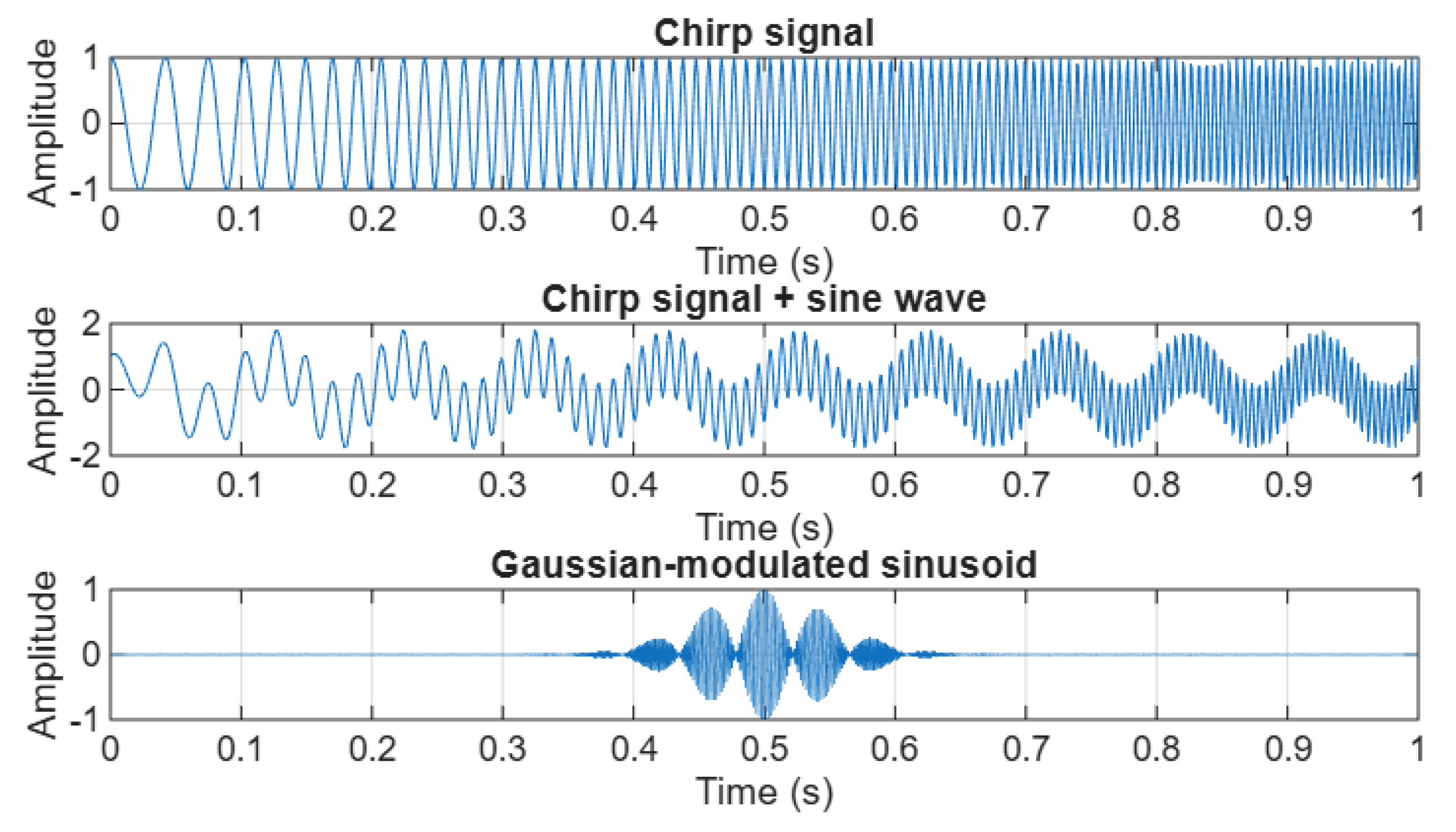
Figure 2.
for different fractional orders.
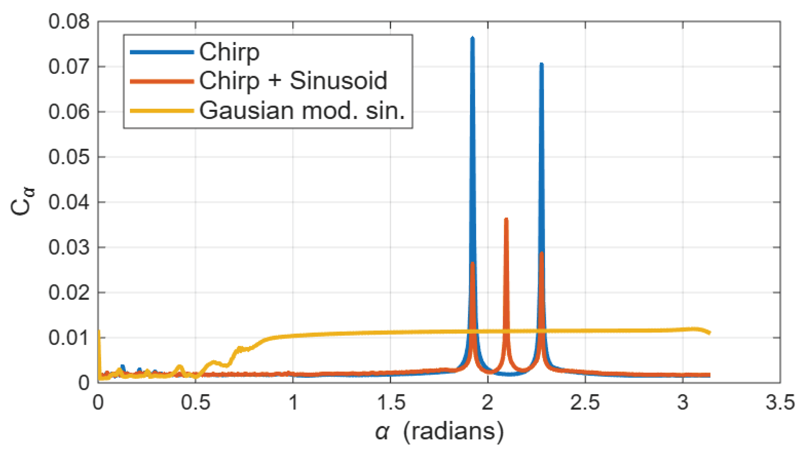
Table 3.
Summary of signals used in the study.
| Signal | Mat. Expression | Parameters / Notes |
|---|---|---|
| (i) | ||
| (ii) | ||
| (iii) | , | |
| G. envelope centered at |
Disclaimer/Publisher’s Note: The statements, opinions and data contained in all publications are solely those of the individual author(s) and contributor(s) and not of MDPI and/or the editor(s). MDPI and/or the editor(s) disclaim responsibility for any injury to people or property resulting from any ideas, methods, instructions or products referred to in the content. |
© 2025 by the authors. Licensee MDPI, Basel, Switzerland. This article is an open access article distributed under the terms and conditions of the Creative Commons Attribution (CC BY) license (https://creativecommons.org/licenses/by/4.0/).
Copyright: This open access article is published under a Creative Commons CC BY 4.0 license, which permit the free download, distribution, and reuse, provided that the author and preprint are cited in any reuse.


