Submitted:
06 October 2025
Posted:
07 October 2025
You are already at the latest version
Abstract
The evaluation of groundwater recharge is a main issue in karst regions threatened by meteorological drought. Since June 2017, a measurement site consisting of a micrometeorological station and two monitoring wells is operational in the Salento peninsula (southern Italy) with the aim of establishing the relationships between groundwater fluctuations and weather forcings over different time scales. In this paper, using inductive reasoning, some insight and knowledge into the local recharge dynamics and monitoring well responses are gained. The results are as follows: (1) short-term fluctuations in water table well are due to atmospheric pressure changes combined or not with precipitation inputs; (2) seasonal fluctuations are apparently controlled by monthly cumulative rainfall; (3) long-term groundwater fluctuations seems to be strictly related to the meteorological variability. As research continues, the site may become a reference for exploring the response of the groundwater reservoir to ongoing climate change.
Keywords:
monitoring well
; hydrograph interpretation
; site hydrostratigraphy
; vadose zone
; well barometric response
; aquifer recharge
1. Introduction
Groundwater levels in wells change in response to a number of processes and over different time scales. Short-term fluctuations occur as a result of precipitation, barometric-pressure changes, pumping, natural or artificial recharge, and other causes. Mid-term fluctuations in groundwater levels are usually due to the seasonality of evapotranspiration, rain infiltration, and irrigation. Finally, long-term (years to decades) fluctuations are caused by meteorological variability, climate changes and extensive human activities (e.g., diffuse extraction, induced recharge, changes in land use) [1,2,3].
Groundwater Recharge (GR) is defined as the entry into a saturated zone of water made available at the water table surface, together with the associated lateral flow within the aquifer [4]. There are several approaches for estimating recharge from groundwater level data, although the most widely issued is the water table fluctuation (WTF) method [1]. Reliable evaluation of GR is crucial in assessing the renewability of groundwater from rain infiltration, especially (but not exclusively) in semi-arid karst regions actually or potentially affected by meteorological drought [4,5,6,7]. Therefore, in different karst regions, measurement sites allowing to determine partitioning of precipitation into soil moisture, evapotranspiration, and GR are in operation (cf., e.g., Refs. [8,9]).
A measurement site, consisting of a micrometeorological station and two monitoring wells tapping an unconfined groundwater reservoir, operates since June 2017 within the Ecotekne Campus of the University of Salento (Salento peninsula, Italy) [10]. The collected time series were used to explore the multi-annual (2017-2022) relationships between groundwater fluctuation and vadose percolation [11]. With the aim of establishing the basis for a GR evaluation, this study tries to inductively identify the processes causing short- and mid-term WTFs in the monitoring wells. The multi-annual trend of the groundwater level is then investigated to gain insights on the influence of meteorological variability. A comparison of the collected WTF time series with a dataset recorded in a different locality of the Salento peninsula raises some questions regarding the behavior of the regional hydrogeological system. Finally, future research goals are discussed.
2. Study Area and Site Description
2.1. Hydrogeological and Climate Setting
The Salento peninsula is the southeastern tip of Italy and belongs to the administrative region of Apulia (Figure 1). Its groundwater is contained in a complex hydrogeological system and provides about 80% of residential water demand. This system consists of a deep coastal Cretaceous Aquifer (CA) and several shallow Tertiary/Quaternary aquifers bounded by aquitards and aquicludes [12,13,14].
The freshwater contained in the CA and the intruding seawater meet and mix in a transition (brackish) zone (Figure 1). GR occurs throughout the rainy season (autumn-winter), while no effective input is expected in the dry season (spring–summer). This latter includes the recession period during which net infiltration is hampered by high evapotranspiration rates and low soil moisture contents [11,16,17].
Since the Upper Cretaceous, different phases of extensional tectonics faulted the developing sedimentary bedrock, resulting in a NW-SE horst and graben structure. The stratigraphic sequences are vertically and laterally variable and control the groundwater circulation, especially the variations in conductivity and inter aquifer transfers [14,18,19]. As a whole, the hydrogeological system of the Salento peninsula should consequently behave as a compartmentalized aquifer. Carbonate rocks prevail in the study area and, therefore, karst features are considered to play an important role in determining the surface water and groundwater flow patterns [15,20,21,22]. The vegetation cover is characterized by Mediterranean scrub-land with several coastal pine forests and few residual oak woods, and agricultural areas with large extensions of olive groves and vineyards, and smaller irrigated patches of crops and orchards [23].
Salento is a warm temperate region with dry-hot summers (Csa climate type [24]), mild-wet winters and about 650 mm of average annual rainfall in the last decades [25,26]. It is highly responsive to climate variability, thus severe possible incoming effects on water resources could happen in a near future [27,28]. The peninsula is mainly exposed to northwesterly winds generally turning to southwesterly with approaching Atlantic lows. These latter, together with northeastern cold outbreaks, are responsible for most precipitating events. It has been found that an abrupt falling in atmospheric pressure usually precedes the approach of a weather system associated with precipitation and precipitation is strongly correlated with decreasing pressure [11,23]. Therefore, the short-term effects of these meteorological parameters on WTFs may be hard to disentangle.
In the last decades, the annual precipitation over the Salento peninsula has slightly decreased while temperature shows statistically significant increasing tendencies especially in summer [29]. The increase in minimum temperature was about two times the global trend while the reference evapotranspiration increased considerably (15–20 mm per decade) [30]. Again, since at least the 80s, drought periods of 50 consecutive days are frequent in the summer (July-August) months [25]. The Salento peninsula must therefore be considered a semi-arid area threatened by meteorological drought [31].
2.2. The Measurement Site
The site of the Ecotekne Campus (Figure 1) was selected based on practical criteria (see Appendix A for details). The micrometeorological station (Figure 2) is active since 2002 and collects data based on half-hour averages that are stored in local memory and then transferred to the web data base [26]. The monitoring wells (named Fiorini, FW, and Benessere, BW, Figure 2) have large diameter (1.4 m FW; 1.1 m BW) and were hand-dug more than a century ago to provide water for agriculture and rural settlements. They tap a groundwater reservoir named MACES, an acronym that means Miocene Aquifer of the Central-Eastern Salento. MACES is mainly made by Middle-Late Miocene calcarenitic calcilutites [14,32]. It is a heterogeneous and low permeable aquifer somewhere affected by karst dissolution that can locally increase its hydraulic conductivity (Appendix A).
The site is located within a graben depression in a suburban environment (Figure 1). Oligocene to Early Miocene units form an aquiclude separating CA from MACES. About 60 years ago, before suburbanization and groundwater exploitation (see Appendix A), well tests had shown that the aquifers had the same piezometric head (i.e., MACES was in hydraulic equilibrium with CA) [11]. Towards the northwest, the aquiclude becomes thinner and thinner and finally disappears (lateral pinch-out of beds), therefore MACES recharges CA. The inter-aquifer leakage (i.e., the drainage of the shallow aquifer into the deep aquifer) occurs also towards the southwest and northeast by means of horst-graben fault systems (Figure 1). Due this hydrogeological setting, the groundwater elevation of CA forms the local base level (i.e., the lowest level that can occur from groundwater flow; cf. Ref. [33]) of MACES [34]. Inside the graben, the Miocene rocks are covered by Quaternary rocks (coarse calcarenite, silty-clay and sands, from the bottom to the top of the succession) [35].
The water table of MACES lies at a depth of 20–22 m below the ground in the Ecotekne Campus area, while the monitoring wells are about 25 m deep [11]. The vadose zone consists of two set of layers. The upper part is made by Quaternary coarse calcarenite rocks, while the lower part by Miocene calcarenitic-calcilutite rocks (left inset of Figure 2). In absence of dissolution-enlarged fractures, these latter must be considered low-permeability layers. Given the above, it was early assumed that barometric changes, vadose/shaft flow, and well bore effects could affect the groundwater data (see Appendixes A and B for more details).
Manual measurements of groundwater level (as water-table depth below the well head, see Appendix A for the measurement-scheme) began in June 2017 for FW, and in June 2018 for BW. They have been taken 2-2.5 times per week using a water-table meter (Boviar GST-FR100). The frequency of measurement was established during the first months of monitoring, taking into account the device sensitivity (0.5 cm) and the occurrence of WTFs. It proved to be suitable for understanding the seasonal, annual, and multi-year relationships of the groundwater level with the rainfall inputs (Section 4). In autumn 2021, BW was temporarily equipped with HC--SR04 ultrasonic detection sensors controlled by an Arduino board. Such an instrumentation system was designed to several purposes, including testing manual measurements (Appendix A).
3. Method
For gaining insight and knowledge on the local recharge dynamics and well monitoring response, the relationships between observed WTFs and meteorological data have been investigated by inductive reasoning. This method was used several times to infer the causes of groundwater fluctuations in the short and medium term, with results also of general interest for aquifer and unsaturated zone hydraulics. The works of Yusa (1969) on Beppu site (Japan) and of Weeks (1979) on Lubbok site (Texas, USA) have been earlier observational studies on the effects produced by the barometric-pressure changes in monitored wells [36,37]. Later, the inferences obtained from the comparison of water table levels and meteorological series were used mainly as the basis for analytical investigations [see, e.g., 23,38].
Inductive reasoning involves generating hypotheses based on systematic observations and data examination. Each inductive inference start from assumptions on data, and end in conclusions that extend beyond the data. The quantitative analysis of observed phenomena, the testing of hypothesis, and the inference of the best explanation form the basis of this method. However, researchers are “unable to agree on the correct systematization of induction” [39, p. 647]. Indeed, different inference strategies can be used in relation to the emerging issues while inductive inference may only be valid locally [39,40,41].
Multi-year observations of WTFs can be relevant in characterizing some subsurface conditions. According to Butler et al. 2021 [42], different insights can be gleaned from long-term hydrographs including the nature of GR and possible preferential connections between monitoring and pumping wells. Particular emphasis is given by these authors to the different manners to interpret WTFs with reference to the available hydrogeological knowledge.
A comparative analysis of long-term hydrographs carried out at selected sites has been used to investigate the relationships between precipitation and GR in climate perspective (see, e.g., Refs. [43,44,45]). Inductive inferences on well responses can be also useful for hydrogeological characterization (see, e.g., Refs. [46,47]). Therefore, the use of systematic observations and data evaluation in the framework of inductive reasoning can lead to various research developments.
In agreement with the literature, the standard hydrological year (from 1 October to 30 September in temperate/mid-latitudes of the Northern Hemisphere) is herein used for subdividing the time series data and investigating the inter-annual variability. However, in the study area, the rainy season can begin as early as early September, marking the end of the recession period in advance of the end of the hydrological year. The average of the water table levels measured in the drought July-August period (ASL, Average Summer Level; see Section 2.1) is used as a proxy of the recession level at the time of the peak [1,48]).
The initial project envisaged monitoring only the FW (Figure 2). At that time, precipitation was thought to be the first cause of WTFs. However, considering the local hydrostratigraphy (Section 2.2 and Appendixes A and B), the infiltration and groundwater flows were expected to be complex. Hypotheses for interpreting the hydrographs were made during the first two observed hydrological years (2017-2018 and 2018-2019). They were then tested by analyzing and comparing the WTFs with the weather data in the process of being acquired.
4. Results
The observations allow to identify the processes causing WTFs in the monitoring wells over different time scales. In this way, useful elements for the characterization of the site were obtained. This section is subdivided into subsections on: emerging issues and working hypotheses (Section 4.1); investigation on the effect of atmospheric pressure changes (Section 4.2); observations on seasonal fluctuations (Section 4.3) and multi-annual trend of groundwater level (Section 4.4).
4.1. First Observations and Hydrograph Interpretations
The outlined complexity of the WTF pattern (Section 2.2) was confirmed soon and, as an example, Figure 3 can be considered. Observed high daily increases in water table level (see e.g., the increase of 3 cm from 5 to 6 March 2018) could be caused by a fast infiltration component through enlarged discontinuities or karst conduits. On the other hand, water table and barometric-pressure changes appeared inversely related (with a time delay among the peaks of about 1 week, see Figure 3). This delayed inverse correlation has since been frequently observed, becoming a reference point for the research.
With the beginning of the irrigation season, the issue of the possible influence of groundwater exploitation on the WTFs was faced. This potential noise problem could happen especially in the presence of preferential connections (karstified fractures and/or bedding planes) between FW and pumping wells. April 2018 was particularly dry (less than 5 mm of total rainfall) and in the meantime the water table level in FW dropped by 30 cm (Figure 4). Barometric pressure decreased by about 12 mbar until 11 April, so WF level was expected to increase over the next 7-10 days. Instead, the water level continued to fall and the assumption of a preferential hydraulic connection with one or more pumping wells took shape. Differently, the atmospheric pressure peak recorded on 18 April could have contributed to the subsequent lowering of the water table. Anyway, it was clear that a single time series of WTF data did not allow us to evaluate the different possible hypotheses.
Again, during May 2018, there were 2 heavy rains (8 and 23 May). After small increases, the water table continued to fall (Figure 4). Consequently, to obtain more robust insights for interpreting the data, it was decided to start monitoring a second well from June 2018 (BW, see Figure 2 for its location). As can be observed in Figure 5 (top side), the fluctuations in the two wells do not show substantial differences (the two lines fit almost perfectly). Given this evidence, it was inferred that: (1) the monitoring wells do not intersect hydraulically active conduits connected, in turn, to pumping wells or karst shafts; and (2) MACES appears to be not influenced by secondary permeability (cf. Appendix A), at least in the area of the measurement site. Otherwise the hydrographs would have shown some differences.
In Figure 5 (bottom side), the difference in water table elevation (BW elevation minus FW elevation) for the selected period is shown. This difference ranges from 0.12 to 0.06 m in the considered period and will not change in the following years. It is also shows that the difference in water table elevation between the two monitoring wells decreases with severe weather conditions. In other words, the level in the FW increases (and also decreases, see below) more and faster than in the BW. This has been a constant feature up to now and may be due to different well bore storage (Section 5.3).
4.2. Atmospheric Pressure Change Effect
During the hydrological years from 2019 to 2023, at the end of long drought periods (some weeks) and several days before the rainfall occurrence, the rising of the water table was observed many times. The most likely explanation for the cause was thought to be the decrease in atmospheric pressure that occurred several days before the precipitation. Considering the early observations (Section 4.1), a positive peak of the water table should correspond to a negative peak of the atmospheric pressure, and vice versa. However, the frequency of the water table measurements (2-2.5 per week, see Section 2.2.) did not allow for reliable conclusions. Thus, during the hydrological years 2023-2024 and 2024-2025, the frequency of the measurements in the monitored wells was temporarily increased (up to 5 days per week). These years have been characterized by dissimilar weather conditions, especially in the winter period, allowing us to observe the fluctuations of the water table under different forcing conditions.
The 2023-2024 winter in Salento peninsula was relatively dry with less than 70 mm of rain recorded by the IMS (Figure 2) from 26 December to 1 March. The atmospheric pressure was characterized by wide fluctuations (up to 30 mbar in 10 days, see Figure 6).
Considering the period from the end of December 2023 to the beginning of March 2024, three apparent cause-effect relationships were found between atmospheric pressure changes and WTFs (Figure 7). The time lags between an atmospheric pressure peak and the corresponding water table peak were about of 1 week. The first 2024 weather system that affected the Salento peninsula was associated with a fall of pressure from 1020 to 990 mbar (28 December–6 January) and 3 days of low precipitation (6-8 January; 13,8 mm of cumulative rain). This event corresponded to a rise in the water table of about 10 cm in FW and 8 cm in BW. It should also be noted that while the rain of January 20 did not cause an assessable rise in water table well, the rise in levels from 6 to 20 February occurred without contribution of concomitant rainfall.
The 2024-2025 winter in the Salento peninsula was moderately wet. The cumulative rainfall recorded by IMS from 28 December to 20 March was almost 170 mm, while the atmospheric pressure was characterized by smaller fluctuations than in the previous winter (Figure 7). During this time interval, the rising of the water table several days before the rainfall occurrence was repeatedly observed (e.g., 8 January, 14 February, and 12 March, Figure 7). Despite the increase in the frequency of the water table measurement, the maximum/minimum has not always been identified precisely (see dotted lines in Figure 7). Also, the FW peak sometimes preceded the BW peak.
The first 2025 weather system was associated with a fall of pressure of 25 mbar (2-12 January) and 3 days of prolonged precipitation (11-13 January; 64,8 mm of cumulative rain). This event corresponded to a rise in the water table of 13 cm in FW and 10 in BW. Comparing data collected during the first adverse meteorological conditions occurred in 2024 and 2025 respectively, in the short-term the rainfall infiltration through the vadose zone appears to contribute less to the rise in the water table than the drop in barometric pressure (Section 5.1). Even the heavy rain of February 2 (37,2 mm) seems to have had no perceptible effect on the concomitant rise of the water table (Figure 7). Again, the rise in the water table observed from March 9 to 18 cannot be correlated with any rainfall.
4.3. Seasonal Groundwater Fluctuations
Seasonal fluctuations in groundwater level occurred over the 8 years of observation. As expected, higher average levels were observed during the rainy season (autumn-winter) and lower average levels during the dry season (spring-summer). In FW, the difference between the Highest Rainy Season Level (HRSL) and the Lowest Dry Season Level (LDSL) ranged between 0.19 and 0.35 m (Table 1). Similar values were observed in BW. To show the general features of the mid-term fluctuations, years with contrasting rainfall patterns are considered in what follows.
The 2017-2018 was the wettest year (845 mm of rain) throughout the observation period. A level difference of 0.34 m was found, almost the largest (Table 1). In January-March 2018, about half of the annual precipitation fell, and the highest water table level was recorded after the wettest month (late in the autumn-winter semester, Figure 8). During groundwater recession, water level dropped and then continued to fluctuate until the summer.
The 2023-2024 was, together whit 2021-2022, the driest hydrological year (512 mm of rain) throughout the observation period. A difference 0.23 m was found between HRSL and LDSL (Table 1). Despite low autumn rainfall, the highest levels were observed in the period December-January. In mid- January, the water table dropped abruptly due to sharp increases in barometric pressure (Section 4.2, Figure 6). During the rest of the hydrological year (throughout the recession period), it decreased and oscillated until July-August. Finally, September 2024 was particularly rainy and unsettled (the next hydrological year seemed to have started early) causing a significant rise in groundwater level (Figure 9).
Considering the above observations, groundwater fluctuations are apparently correlated to cumulative precipitation on the mid-term scale at the Ecotekne Campus site. Polynomial trend lines can be used as proxies of these periodic changes in water table level to highlight their seasonality (Figure 8 and Figure 9).
4.4. Multi-Annual Trend of Groundwater Level
The 8-year linear trend of the water table level has a negative slope (red line in Figure 10), thus suggesting a decline of the groundwater stored in MACES over the considered period (Section 5.3). However, during 2022-2023 the water table has risen, reaching a higher average summer level than the previous year (marked by an arrow in Figure 10; see also the coincident LDSL increase in Table 1). The 4th order polynomial curve (black line in Figure 10) highlights a multi-annual fluctuation.
To explain the above long-term fluctuation, the variations in annual precipitation can be considered. Cumulative rainfall decreased by 60% from 2017-2018 to 2021-2022 (Table 2), with values lower than the multi-decadal average (i.e., 650 mm, see Section 2.1) for 3 consecutive years. Instead, in 2022-2023, annual precipitation exceeded the average by 20%, increasing by 50% compared to the previous year. Over the last two hydrological years, annual precipitation has once again fallen below average (Table 2).
The LDSL (Table 1) may be strongly influenced by the effect of atmospheric pressure (Section 4.2). A better proxy of the groundwater level at the end of the recession period is the ASL parameter, that is the average of the water table levels measured in the drought July-August period (cf. Section 2.1, Section 3, Section 4.3). The annual groundwater level change (AGLC, Table 2, columns 4 and 5) is calculated as the difference in the ASL between two subsequent years. From October 2017 to September 2022 ASL decreased year by year (Table 2). In 2022 summer, ASL returned to the level of 2020 summer, recovering over 0.1 m (see Table 2). Finally, this recovery was reversed in the last two hydrological years.
Using this evidence, some insights into the climate relevance of the above multi-annual trend, including inter-annual recharge variability, can be drawn (Section 5.3).
5. Discussion
The study of aquifer recharge in semi-arid regions is particularly challenging due to several environmental conditions [8,49,50]. In addition, lithological heterogeneity in karst vadose zone can produce complex infiltration dynamics influencing both the timing and extent of GR [51,52]. On the other hand, WTFs may be out of phase with atmospheric pressure changes where low-permeability layers are present in saturated zone [37]. Thus, during the monitoring activity, special attention was given to infer insights and knowledge on these issues.
Considering the characteristics of the Ecotekne Campus site, a single monitoring well would not have been enough to verify some basic hydrogeological conditions (Section 2.2, Appendix A). Differently, the use of two wells shed light on both the hydraulic connectivity and the type of permeability of the aquifer. The hydrographs match almost perfectly, so connections between monitoring wells and pumping wells and karst shafts can be reasonably ruled out; meanwhile, MACES appears to be controlled by primary rather than secondary permeability (Section 4.1). Once enough evidence about these aspects was gathered, the main effort was focused on the short- and mid-term meteorological forcings (Section 4.2, Section 4.3). Finally, attention is beginning to shift to the multi-annual trend of groundwater level (Section 4.4). For an overview of the ongoing observational work, the weather forcings over different time scales (Section 5.1), the significance of the site in the regional context (Section 5.2.) and the future research goals (Section 5.3) are discussed below.
5.1. Weather Forcings over Different Time Scales
A short-term influence of the atmospheric pressure changes on WTFs was soon hypothesized (Section 4.1; Appendix B) and then extensively explored (Section 4.2). In both monitoring wells, water table rise was frequently observed during an atmospheric pressure drop and several days before precipitation occurred, even after long periods of drought. Low values (negative peaks) of atmospheric pressure preceding the approach of unsettled weather conditions were many times found about a week before positive peaks in water table level. Likewise, high values (positive peaks) of atmospheric pressure bringing settled weather conditions were found about a week before negative peaks in water table level. Finally, the increase in the water table level after the drop in atmospheric pressure occurred even in the absence of precipitation (Section 4.2). A strong control of short-term atmospheric pressure variations on WTFs is the best explanation for these observed phenomena.
In literature there are several studies on the barometric pressure effects in unconfined aquifers (see, e.g., Refs. [37,38,53].) However, they regard small diameter drilled wells with blind casings in the vadose zone and slotted screens in the whole saturated zone. Rise and fall of water level in wells tapping unconfined groundwater reservoirs were described as delayed responses to atmospheric pressure variations, while the basis to account for these transient effects can be provided by the calculation of the barometric response characteristics for individual wells [38,53]. These delayed responses are triggered by the crossing of barometric pressure change through the vadose zone that causes a pressure potential gradient between the wells and the surrounding aquifer. The equalization of pressure is not instantaneous because of the time required for radial groundwater flow into and out of the wells [54,55]. The time delay depends on the aquifer properties (i.e., hydraulic conductivity, specific storage, saturated thickness) and existing well/borehole conditions (i.e., well bore storage, well skin effects, discrete vertical interval in which the well is open to the aquifer). Low values of hydraulic conductivity and pneumatic diffusivity can therefore significantly increasing the time lag of the well response (cf. Refs. [38,56]).
Since the onset of precipitation has always been preceded by a decrease in atmospheric pressure, there are no observations that allow us to inductively establish the short-term influence of rain on the water table. However, the comparison between the measurements collected during the winter of 2023-2024 and the winter of 2024-2025 (Section 4.2), allowed us to roughly assess to what extent precipitation input could overlap with barometric pressure input in determining water table rise (see Appendix A for the infiltration pathway and other details). Two examples are enough to understand this feature. In FW, 10 cm and 13 cm of water table increase were measured after the precipitation of 6-8 January 2024 and 11-13 January 2025, respectively. Since the second event was much rainier than the first (cf. Figure 6 and Figure 7), we argue that, on a weekly scale, rainfall infiltration can only make a little contribution to the water table rise (likely less than 20%). There was no evidence of the contrary of this finding throughout the observation period.
Inductive reasoning can also help us to gain insights into the mid-term effect of precipitation on water table rise. Observations on seasonal fluctuations are useful for this purpose (Section 4.3). Comparing the graphs in Figure 8 and Figure 9, or their polynomial curves (which are more easily readable, cf., e.g., Refs. [57,58]), it can be deduced that the highest mean levels occur after the wettest month of the autumn-winter period (February in the 2017-2018 hydrological year, and November in the 2023-2024 hydrological year). Thus, differently from the short-term fluctuations, the mid-term fluctuations observed in the monitoring wells would appear to be controlled by rainfall infiltration (Section 4.3). It can be argued that most of the infiltrated rainwater would take at least 1 month to reach the aquifer (Figure 8 and Figure 9).
The use of stochastic models could help to reach more confident conclusions [59,60,61]. An attempt to obtain further information on the short- and mid-term processes herein described has been performed by two complementary black box approaches [62]. In particular, a Langevin equation has been used to investigate the correlation functions in presence of time-correlated forcing, and a response function model has been used to solve least square regressions for water table cross-correlograms with precipitation and atmospheric pressure in both time and frequency domain. The results indicate a time response of about one week to be attributed to the correlations between the meteoric forcings, and a response duration of about 80 days (with a delay between 30 and 60 days) to be attributed to rainfall infiltration [62]. These findings are consistent with the inductive explanations given above.
Regarding the long-term changes in groundwater level, 8 years of monitoring is not an appropriate length of time for a reliable evaluation. However, the data collected to date allow us to formulate one hypothesis. The downward trend in the water table (Figure 10) was accompanied by a decreasing tendency in annual precipitation (Table 2). The hydrological year 2022-2023 was an exception, recording increases in both mean groundwater level and cumulative precipitation (Section 4.4). It can therefore be assumed that the monitored water table could be responsive to inter-annual change in precipitation. Based on the data collected so far, there is a direct nonlinear relationship between the annual variation in precipitation and that of the ASL parameter (Figure 11). Continuous meteorological and hydrogeological monitoring will allow for a larger database.
GR changes in semi-arid regions are expected to be significantly affected by variations in evapotranspiration rate [63,64]. According to Delle Rose and Martano 2023 [11], in the hydrological years 2017-2018 to 2021-2022, real evapotranspiration showed a downward trend, although not very significant. In this five-year period, the decrease in precipitation recorded at the Ecotekne Campus (Table 2) was therefore accompanied by a slight decrease in evapotranspiration. Further data collecting and analyzing is required to properly investigate this issue (Section 5.3).
5.2. Relevance of the Site in the Regional Context
The usefulness of a hydrological measurement site depends on several requirements, including the presence of common characteristics in the region where the site is located. In the Salento peninsula, suburban areas prevail over urban ones and those intended for agricultural-irrigation purposes [65]. The zones characterized by low-density residential neighborhoods, limited infrastructure, sparse wild vegetation, and minimal agricultural activity, such as the Ecotekne Campus, constitute the dominant landscape of the region. From this perspective, the monitoring site, although chosen for simple practical reasons (Section 2.2), is truly typical. Also the vadose zone within the measurement site, composed of high-permeability layers superimposed on low-permeability layers, is characteristic in the region. Several conditions present in the Ecotekne Campus are therefore common in the study region, as suggested in literature for the usefulness of the hydrological observation sites [8,9].
To properly assess how representative the Ecotekne Campus is for near-surface hydrogeology, several well hydrographs scattered throughout the Salento peninsula are needed. Since a decades-long process of groundwater depletion and salinization affects the regional water resources [12,20,66], the Apulia water authority periodically funds and leads well monitoring activities. Such campaigns are considered essential for water resources protection and management. The monitoring measurements of the Tiziano Project (2007-2011) are the latest publicly available data on which researchers have carried out studies [23,67]. For the above reasons, it is not currently possible to compare the Ecotekne Campus datasets with hydrological datasets of the regional water authority.
To our knowledge, the only research conducted on a time series of groundwater level recorded in the Salento peninsula since 2017 is the one reported by Leins et al., 2023 for the CA [68]. This series starts from November 20, 2017 and ends on October 24 of the following year. It can then be compared with the measurements taken in FW (Section 2.2). As can be observed in Figure 12, the two hydrographs are very similar and only minor differences are evident comparing the curves. This similarity is apparent despite the striking differences in data acquisition techniques (one manual, the other automatic) and frequency measurements (2-2.5 measures per week at the Ecotekne Campus, 1 measure per hour at the comparison site).
To explore the possible implications of this similarity, some essential features of the measurement site of Leins et al. 2023 [68] must be first drawn. It consists on an automatic multiparameter probe placed below the water table inside a 70 m deep karst sinkhole (local name: Vora Bosco; see Figure 1 for its location). This sinkhole drains the ephemeral runoff of an endorheic basin of approximately 1 square km (it acts as a recharge point) and allows the speleologists to reach the water table of the regional deep aquifer (Section 2.1). Unfortunately, due to the severe heavy rainfall on 22-23 October 2018, and the resulting sinkhole flooding, all installed instrumentations were lost [68].
The 22-23 October 2018 rainfall event also caused the largest increase in water table elevation (10.5 cm in FW and 6.5 cm in BW, see Figure 5) during the first two years of monitoring at Ecotekne Campus. A convective cloud system bringing a huge localized precipitation in short time characterized such an event [69]. The ISAC-CNR micrometeorological station (IMS in Figure 2) recorded 40 mm of rain in 3 hours. Other meteorological stations scattered over the region and managed by the civil protection authority recorded up to 245 mm in two days (data from Annali Idrologici of “Ufficio Idrografico e Mareografico” [70]). Different endorheic areas were flooded for several days suffering significant damage [69], including the basin of Vora Bosco [68].
At least two hypotheses can be made to explain the apparent correlation between the hydrographs in Figure 12: 1) MACES and CA behave, at a regional scale, as a porous aquifer rather than as a compartmentalized aquifer system; 2) MACES is locally well connected to CA and its water table reaches the base level in short time. Both hypotheses find support in the literature (Appendix C). The evaluation of these hypotheses can give further relevance to the research at the Ecotekne Campus site.
5.3. Future Research Goals
The observations carried out at Ecotekne Campus allowed a better knowledge into short- and mid-term WTFs, local recharge dynamics, and response of wells to weather forcings. They also raised a number of issues to be addressed as research continues. Given that the long-term aim of the research is to obtain a reliable assessment of GR, the main efforts will be directed towards the achievement of this result.
Different approaches are used to estimate GR based on groundwater level data. The WTF method is widely used due to its advantages of low cost, few required data and simple calculation [1,15,71,72]. However, the accuracy of the WTF method could limited because of signal lag, attenuation and uncertainties, especially from barometric pressure effect, unsaturated drainage, and lateral flow [73,74,75]. Considering the characteristics of the Ecotekne Campus, the applicability of the WTF method to the collected data is constrained to mid-term time scales. Furthermore, the specific yield of MACES has not yet been calculated. Due to the importance of this parameter for GR evaluation, it should be determined using different procedures [76,77]. Aside from the reliability of the specific yield calculation, it will eventually be appropriate to apply different methods of GR estimation, including those not based on WTF, relying on consistency in results.
Given that groundwater depletion is a global concern [78,79], multi-annual trend in groundwater level is gaining widespread interest as a practical tool for initial hydrological evaluation. As an example, for assessing the quantitative status of an aquifer, the World Meteorological Organization proposes to use decadal trends of well hydrographs together with the rank of the mean groundwater level in a given year [80, pp. 12-13]. The trend can be “rising”, “stable” or “declining” while the rank, determined by percentile calculation, can be “above normal”, “normal”, or “below normal” in comparison to the average decadal level [81]. This methodology could be applied to MACES in the near future, possibly increasing the number of observed wells and making use of automatic groundwater level monitoring instruments. Furthermore, long-term hydrographs of selected sites are used to investigate the relationships between climate variability and GR (see, e.g., Refs [43,44,45]). By extending the observations on the Ecotekne Campus site over time, a dataset suitable for such an investigation could be available [51,82].
Along with a decreasing trend, the groundwater level data from the last 8 years described above (Section 4.4) show a significant inter-annual variability directly related to changes in precipitation (Section 5.1). Based on the data collected so far, this relationship is not linear (Figure 11). A high inter-annual recharge variability is typical in semi-arid regions [83,84,85]. Precipitation variability is thought to explain up to 80% of inter-annual recharge variability [86]. However, since both the minimum temperature and reference evapotranspiration increases significantly in the Salento peninsula [30], it will be mandatory to explore the role of evapotranspiration variability for a reliable explanation of recharge variability.
A deeper understanding of the relationships between WTFs and atmospheric pressure changes will be another aim of research. Short-term fluctuations have been found and described through manual measurements of groundwater level taken 2 to 5 times per week. Barometric-pressure changes are inversely related to WTFs, with an average time delay of approximately 1 week. Rainfall infiltration can slightly amplify the effect of this forcing (Section 4.1, Section 4.2). To refine this result, high-resolution WTF data must be collected using automatic sensing and recording instruments. Furthermore, high frequency monitoring is also essential for improving site characterization [47,87]. To achieve these goals and monitor physical-chemical parameters, it is planned to install sensors for data automatic collection within the monitoring wells [88]. The sensors will be controlled by a Raspberry Pi device, while dedicated transmission protocols will allow secure remote data acquisition. Regarding the atmospheric pressure forcing on the water table in the wells, a finer definition of the time delay and a better understanding of the phenomenon are expected. In the meantime, it should be possible to calculate the barometric response function and infer the hydro-geomechanical properties of the site (c.f., e.g., Refs. [38,53,87]).
Again, since water table level increases and decreases at different rates in the two monitoring wells (Section 4.1), it could be investigated whether this is due to different storage characteristics of the wells. Dealing with large diameter wells, several approaches are proposed in the literature to address this problem [89,90,91]. Finally, to test the reliability of the presented results, several analytical and laboratory models may be used (see, e.g., Refs. [92,93,94]), even taking into account the particular lithology of MACES.
6. Conclusions
In this paper, an explanation of the relations between hydrogeological and meteorological data and the hydrological behavior of a measurement site is given by inductive reasoning based on a system of inference. First, some evidence shows that monitoring well levels are not influenced by either pumping or karst flows, which could have hampered the interpretation of WTF time series. On the other hand, the site itself has proven to be representative of the area in which it is located. Short-term variations in water-table levels occur mainly in response to atmospheric pressure changes, while mid-term water table fluctuations are apparently related to recharge due to fall-winter precipitation.
The monitored groundwater level appears to be responsive to the changes in annual precipitation. A direct nonlinear relationship has been found between the annual variations in precipitation and the average summer groundwater level. Furthermore, the negative slope of the groundwater level trend suggests a decline of the monitored groundwater reservoir throughout the 8 years of observations. High frequency monitoring will allow to have a larger database and test the hypotheses outlined here.
Funding
This research received no external funding.
Data Availability Statement
The dataset of the water-table depths taken from 21 June 2017 to 30 September 2025 can be provided by the author upon request. The atmospheric pressure and precipitation time series can be download from the ISAC-CNR Lecce Micrometeorological database (www.basesperimentale.le.isac.cnr.it) upon request.
Acknowledgments
The author would like to thank his colleagues at the ISAC-CNR Office in Lecce (Italy) for their collaboration in data collection and for the constructive discussions on data processing and analysis.
Conflicts of Interest
The author declares no conflicts of interest.
Abbreviations
The following abbreviations are used in this manuscript:
| ASL | Average Summer Level |
| AGLC | Annual Groundwater Level Change |
| APV | Annual Precipitation Variation |
| CA | Cretaceous Aquifer |
| GR | Groundwater Recharge |
| HRSL | Highest Rainy Season Level |
| LDSL | Lowest Dry Season Level |
| MACES | Miocene Aquifer of the Central-Eastern Salento |
| WTF | Water Table Fluctuation |
Appendix A. Site Characteristics
MACES (the groundwater reservoir inside which the monitoring wells are dug, see Section 2.2) is supplied by net infiltration of rainwater and exploited for irrigation and domestic purposes through many licensed and unlicensed wells. In the dry season, it is recharged by irrigation water withdrawn from CA. Unfortunately, the amounts of withdrawal are not known, therefore the hydrogeological balance for MACES can hardly be calculated. The general hydrostratigraphic features can be described with reference to the chrono-lithostratigraphic units recognized in the whole Salento peninsula [19]. However, local geological details influencing rainfall infiltration and aquifer recharge, such as the lithological heterogeneity and the distribution of dissolution-enlarged discontinuities, are scarcely known.
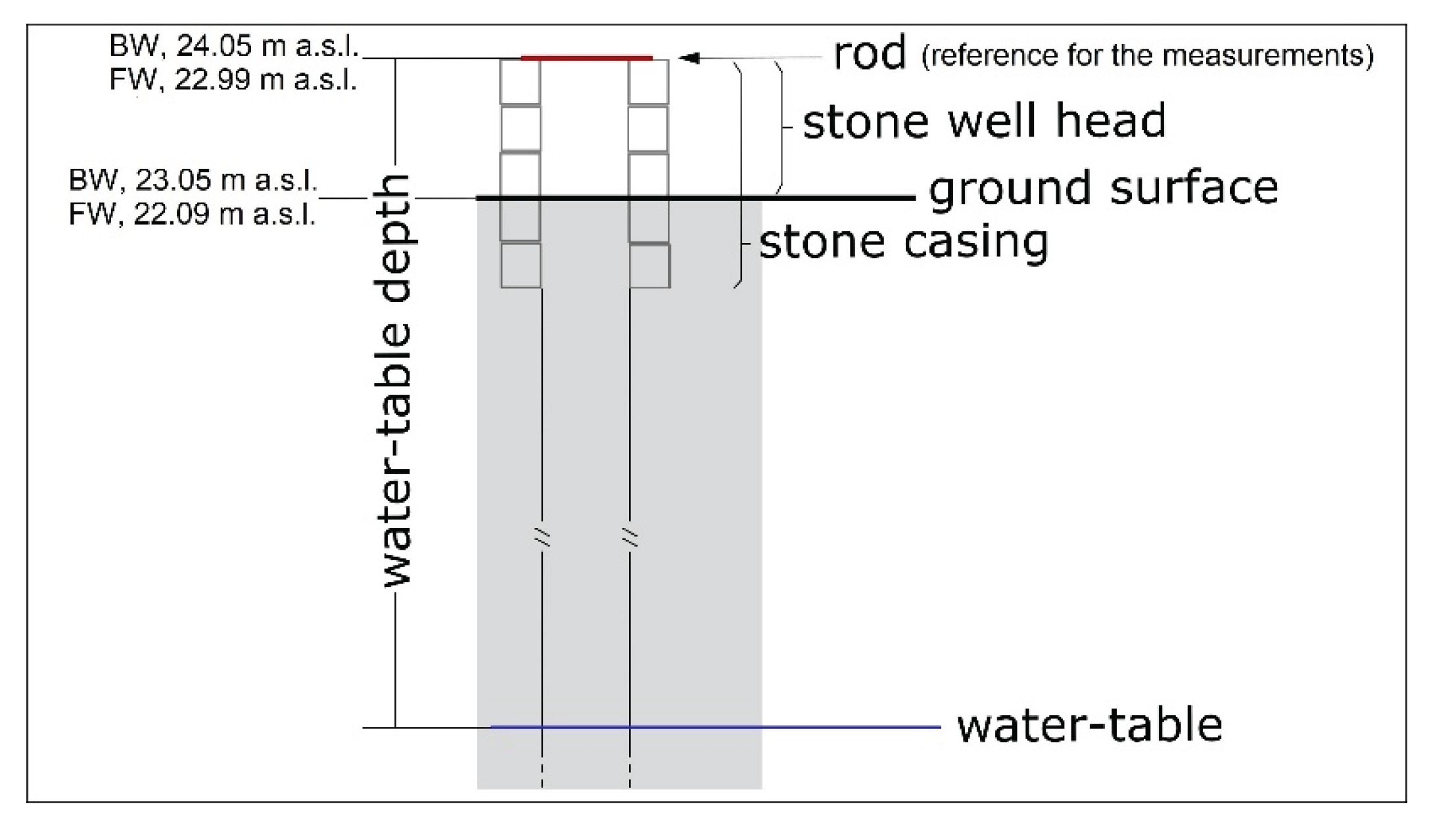
Regarding the choice of the measurement site, the first criterion used was the presence of easily accessible wells in the vicinity of the ISAC-CNR Office (Figure 2). The out of ground casing of the selected wells is made by stone and has a box shape. It allowed to design an inexpensive, simple, and not subjective measurement procedure. The measurements are taken placing a 2 cm thick rod between two opposite sides of the stone casing and using a water-table meter (Figure A1). Since the water-table is clearly visible from above, a simple tape measure can also be used. Measurements performed by different operators have always been found to be equivalent. Such a procedure avoids instrumental errors and the expensive maintenance costs of complex equipment (on the other hand, its main limitation is to take measurements with adverse weather conditions). Moreover, given the proximity of the wells to the micrometeorological station managed by ISAC-CNR (Figure 2), the water table measurements can be related with confidence to the weather measurements. Finally, due the flat topography of the site area, local runoff is negligible. This set of conditions offers the possibility of making a low-cost long-term dataset to study the GR in a climate perspective.
Figure A1.
Scheme for the measurement of the water-table depth (from [11], modified). The altitudes of the ground surface (in meters above sea level) were measured by a GPS device (Leica gps900).
Figure A1.
Scheme for the measurement of the water-table depth (from [11], modified). The altitudes of the ground surface (in meters above sea level) were measured by a GPS device (Leica gps900).
Some physical properties of the Miocene rocks forming MACES and the lower part of its vadose zone (see Section 2.2) can be deduced, in general terms, form literature studies. This layers should have degree of compactness between 0.5 and 0.7, porosity of 0.3–0.45, imbibition capacity of about 10–20% [95], permeability of 10-4–10-5 cm/s [Delle Rose 2001], and a weighted coefficient of infiltration of 0.4 (in a scale of 0 to 1) [19]. Again, Miocene rocks are poorly to moderately fractured. As a whole, their permeability is composed of a primary permeability (apparently homogeneous, associated with the rock porosity) and a secondary permeability (strongly heterogeneous, dictated by a network of sparse sub-vertical fractures randomly enlarged by karst dissolution) [10]. In unsaturated conditions, the Miocene rocks of the Salento peninsula can significantly delay the infiltration of rainwater, especially where they are thick and with very low permeability due to porosity and fracturing [96].
Until the 1960s, the Ecotekne Campus area was extensively exploited for the extraction of building stone. Currently, several quarry walls are exposed. Such exposures allow to observe both the epikarst features and the upper part of the Quaternary rocks. The degree of epikarst development, as evaluated by the frequency and depth of the surface karst features (cf. Refs. [97,98]), is low. However, a number of sub-vertical fractures and sub-horizontal bedding planes are enlarged by karst dissolution and shown apertures of up to several centimeters. No observed fracture shows openings that widen with depth, so it is unlikely that any of them evolve into vertical conduits or karst shafts (cf. Refs. [99,100]). Nevertheless, a set of interconnected discontinuities (fractures and bedding planes) could favor rapid infiltration of rainwater into the wells (Figure A2), similar to the hydraulic behavior of the “complex shafts” of Veress 2019 [101]. In the short term, this process could overlap with the barometric effect in wells (Section 5.1).
Figure A2.
Pattern of the karstified discontinuities affecting the vadose zone. (a) Quarry wall exposure of the Quaternary coarse calcarenite (see text); (b) schematic highlighting of the discontinuities; (c) inferred pattern (not in scale); preferential infiltration pathways are evidenced by arrows.

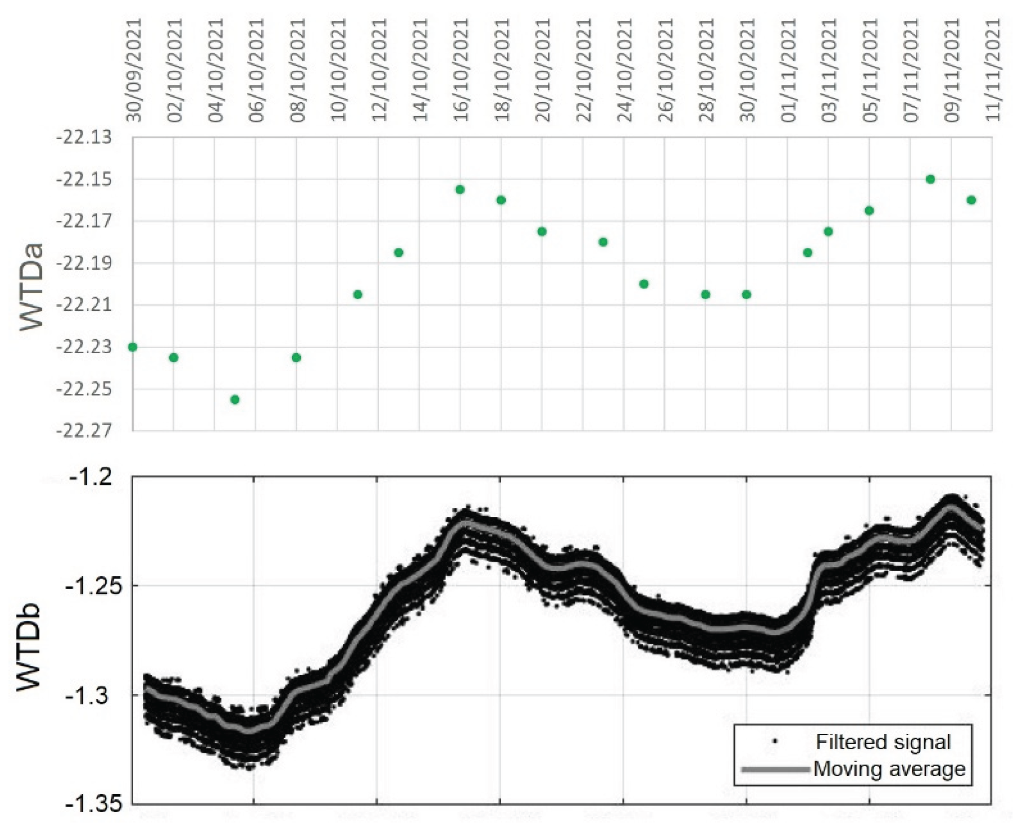
From 30 September 2021 to 11 November 2021, the BW was equipped with an experimental sensor system which collected data every 30 minutes (Section 2.2). Ultrasonic detection sensors for measuring the groundwater level were positioned inside the well, more than 1 m above the water table [102]. As shown in Figure A3, the curve obtained from the automatic measurement fits the trend of the manual measurement. This similarity can be interpreted as a cross-confirmation between the two measurement systems.
Figure A3.
Comparison between water table level measured by HC-SR04 ultrasonic detection sensors (after [102], modified; at the bottom) and the measurement performed manually (at the top). WTDa = water table depth (in m) according to the scheme of Figure A1; WTDb = water table depth (in m) measured by sensors.
Appendix B. Phenomena affecting WTFs
In wells tapping unconfined aquifers, WTFs may be out of phase with barometric changes where the saturated zone consists of poorly permeable rocks, and/or the vadose zone of rocks with low pneumatic diffusivity [37,56]. Such a phenomenon occurs because the movement of the air is slowed by the finite permeability of the unsaturated rocks and by their capacity to store or release soil gas as the pressure change. Therefore, the change in soil gas pressure at the phreatic surface lags that at land surface, while barometric changes are transmitted instantaneously in the wells. This pressure potential gradient produces, in turn, a WTF [38,53]. More in detail, the transmission of atmospheric pressure within the vadose zone is a direct function of its pneumatic diffusivity which depends on the vertical permeability, moisture content and compressibility of the contained gas [37]. Considering the characteristics of the lower part of the vadose zone (Section 2.2), at the beginning of monitoring the effect of barometric-pressure changes on WTFs in wells dug in MACES was believed possible, although not yet investigated.
The WTFs recorded in the Ecotekne Campus could be affected by other processes. A first one concerns the infiltration of the water through the vadose zone. A second one involves the well bore effects. The Quaternary rocks making up the upper part of the vadose zone have high primary permeability (up to 10-2 cm/s) [96]. They are dissected by sub-vertical fractures and sub-horizontal bedding planes both enlarged by karst processes that, apparently, can enhanced the infiltration rate (Appendix A). In the presence of karstified fractures developed along the whole vadose zone, fast infiltration events could occur during severe rainfall (see, e.g., vadose flow and shaft flow, Refs. [97,100,103]). Unfortunately, there are no data to confirm or exclude the presence of significant karstified fractures near the wells. However, the monitoring wells themselves could behave like karst shafts, draining part of the infiltrated water (Appendix A).
Well bore effects include both the bore storage (i.e., the change in water volume in relation to size of the well) and the well skin effects (i.e., a reduction of aquifer permeability near the well). They determine, together with the transmissivity and storativity of the aquifer, the time required for the radial movement of a finite volume of water between the well and the surrounding aquifer in consequence of a barometric pressure change [38,53]. Regarding the measurement site, since the wells were dug by hand and are not screened, the skin effect may be neglected. Instead, due to the large size of the wells (1.1 and 1.4 m in diameter) a significant bore storage effect was expected.
Appendix C. Hypotheses on the Similarity of Hydrographs
The similarity between the hydrographs of FW and Vora Bosco [68] can be explained in at least two ways (see Section 5.2). It is necessary premise that the hydrogeological system of the Salento Peninsula has long been considered to be composed by a main deep aquifer (CA) and a number of shallow aquifers (including MACES) separated from each other (Section 2.1). The horst and graben tectonic setting of the region and the geological evolution would have determined a compartmentalized structure without significant water exchanges (cf., e.g., Refs. [104,105]). However, recent data reanalysis shows that, as a whole, the hydrogeological system of the Salento Peninsula has a great storage capacity, is characterized by a regular percolation of rainwater which recharges the aquifers through delayed pathways, and usually exhibits a slow response to precipitation [67]. Considering this conceptual model, the similarity of the hydrographs in Figure 10 would not be unexpected. The first hypothesis is thus supported.
Regarding the second hypothesis, it must be considered that the Ecotekne Campus site is located within a graben depression which is bounded by normal fault systems [35]. Nothing is known about the hydraulic characteristics of these tectonic structures but some suppositions can be made. Fault systems often introduces permeability heterogeneity and anisotropy, which can have an important impact on the regional groundwater flow. They have the capacity to be hydraulic conduits connecting shallow and deep groundwater reservoirs, even if their core could form barriers to flow [106]. Considering that the flow lines of MACES are directed toward the border of the graben [33] and the water table of MACES was found at the same depth as the water table of CA during groundwater level testing [11], it can be supposed that the normal faults facilitate the inter-aquifer leakage for the case here reported. The search for evidence to support one or the other hypothesis is beyond the scope of this work.
References
- Healy, R.W.; Cook, P.G. Using groundwater levels to estimate recharge. Hydrogeol. J. 2002, 10, 91–109. [Google Scholar] [CrossRef]
- Favreau, G.; Cappelaere, B.; Massuel, S.; Leblanc, M.; Boucher, M.; Boulain, N.; Leduc, C. Land clearing, climate variability, and water resources increase in semiarid southwest Niger: A review. Water Resour. Res. 2009, 45, W00A16. [Google Scholar] [CrossRef]
- Lorenzo-Lacruz, J.; Garcia, C.; Morán-Tejeda, E. Groundwater level responses to precipitation variability in Mediterranean insular aquifers. J. Hydrol. 2017, 552, 516–531. [Google Scholar] [CrossRef]
- Freeze, R.A., Cherry, J.A. Groundwater. Prentice-Hall: Englewood Cliffs, New Jersey, USA, 1979; 604 pp.
- Leduc, C.; Bromley, J.; Schroeter, P. Water table fluctuation and recharge in semi-arid climate: some results of the HAPEX-Sahel hydrodynamic survey (Niger). J. Hydrol. 1997, 188–189, 123–138. [Google Scholar] [CrossRef]
- Touhami, I.; Andreu, J.M.; Chirino, E.; Sanchez, J.R.; Mourahir, H.; Pulido-Bosch, A.; Martinez-Santos, P.; Bellot, J. Recharge estimation of a small karstic aquifer in a semiarid Mediterranean region (southeastern Spian) using a hydrological model. Hydrol. Process. 2013, 27, 165–174. [Google Scholar] [CrossRef]
- Pazola, A. , Shamsudduha, M., French, J., MacDonald, A.M., Abiye, T., Goni, I.B., Taylor, R.G. High-resolution long-term average groundwater recharge in Africa estimated using random forest regression and residual interpolation. Hydrol. Earth Syst. Sci. 2024, 28, 2949–2967. [Google Scholar] [CrossRef]
- F. Ries, J. Lange, S. Schmidt, H. Puhlmann, and M. Sauter. Recharge estimation and soil moisture dynamics in a Mediterranean, semi-arid karst region. Hydrol. Earth Syst. Sci. 2015, 19, 1439–1456. [Google Scholar] [CrossRef]
- R. Berthelin, M. Rinderer, B. Andreo, A. Baker, D. Kilian, G. Leonhardt, A. Lotz, K. Lichtenwoehrer, M. Mudarra, I.Y. Padilla, Pantoja Agreda, F.; Rosolem, R.; Vale, A.; Hartmann, A. A soil moisture monitoring network to characterize karstic recharge and evapotranspiration at five representative sites across the globe. Geosci. Instrum. Method. Data Syst. 2020, 9, 11–23. [Google Scholar]
- Alfio, M.R.; Balacco, G.; Delle Rose, M.; Fidelibus, C.; Martano, P. A hydrometeorological study of groundwater level changes during the covid-19 lockdown year (Salento peninsula, Italy). Sustainability 2022, 14, 1710. [Google Scholar] [CrossRef]
- Delle Rose, M.; Martano, P. Datasets of groundwater level and surface water budget in a central Mediterranean site (21 June 2017–1 October 2022). Data 2023, 8, 38. [Google Scholar] [CrossRef]
- Tadolini, T.; Tulipano, L. The evolution of fresh-water/salt water equilibrium in connection with withdrawals from the coastal carbonate and karst aquifer of the salentine peninsula (southern Italy). Geol. Jaharb. 1981, 29, 69–85. [Google Scholar]
- Tulipano, L. Temperature logs interpretation for the identification of preferential flow pathway in the coastal carbonatic and karstic aquifer of the Salento peninsula (Southern Italy). In Proceedings of the 21 Congress International Association Hydrogeologists, Guilin, China, 10–15 October 1988; volume 2; pp. 956–961. [Google Scholar]
- Delle Rose, M. Sedimentological features of the Plio-Quaternary aquifers of Salento (Puglia). In Memorie Descrittive delle Carta Geologica d’Italia; S.E.L.C.A., Florence, Italy, 2007; volume 76, pp. 137–145.
- Delle Rose, M.; Fidelibus, C.; Martano, P. Assessment of specific yield in karstified fractured rock through the water-budget method. Geosciences 2018, 8, 344. [Google Scholar] [CrossRef]
- Cotecchia, V. Sviluppi della teoria di Ghyben ed Herzberg nello studio idrogeologico dell’alimentazione e dell’impiego delle falde acquifere, con riferimento a quella profonda delle Murge e del Salento. Geotecnica 1958, 6, 301–318. (In Italian) [Google Scholar]
- Portoghese, I.; Uricchio, V.; Vurro, M. A GIS tool for hydrogeological water balance evaluation on a regional scale in semi-arid environments. Comput. Geosci. 2005, 31, 15–27. [Google Scholar] [CrossRef]
- Fidelibus, M.D.; Tulipano, L.; D’Amelio, P. Convective thermal field reconstruction by ordinary kriging in karstic aquifers (Puglia, Italy): geostatistical analysis of anisotropy. In Advances in Research in Karst Media. Environmental Earth Sciences; Andreo, B., Carrasco, F., Durán, J., LaMoreaux, J., Eds.; Springer: Berlin, Heidelberg, Germany, 2010; pp. 203–208. [Google Scholar]
- Giudici, M.; Margiotta, S.; Mazzone, F.; Negri, S.; Vassena, C. Modelling hydrostratigraphy and groundwater flow of a fractured and karst aquifer in a Mediterranean basin (Salento peninsula, southeastern Italy). Environ. Earth Sci. 2012, 67, 1891–1907. [Google Scholar] [CrossRef]
- Cotecchia, V.; Grassi, D.; Polemio, V. Carbonate aquifers in Apulia and seawater intrusion. Giornale di Geologia Applicata 2005, 1, 219–231. [Google Scholar]
- Apollonio, C.; Delle Rose, M.; Fidelibus, C.; Orlanducci, L.; Spasiano, D. Water management problems in a karst flood-prone endorheic basin. Environ. Earth Sci. 2018, 77, 676. [Google Scholar] [CrossRef]
- Rana, G.; Muschitiello, C.; Ferrara, R.M.; Verdiani, G.; Acutis, M. Modelling the groundwater level by water balance: a case study of a Mediterranean karst aquifer of Apulia region (Italy). Ital J. Agrometeorol. 2018, 23, 35–48. [Google Scholar]
- Delle Rose, M.; Martano, P. Infiltration and Short-Time Recharge in Deep Karst Aquifer of the Salento Peninsula (Southern Italy): An Observational Study. Water 2018, 10, 260. [Google Scholar] [CrossRef]
- Peel, M.C.; Finlayson, B.L.; McMahon, T.A. Updated world map of the Köppen-Geiger climate classification. Hydrol. Earth Syst. Sci. 2007, 11, 1633–1644. [Google Scholar] [CrossRef]
- Zito, G.; Ruggiero, L.; Zuanni, F. Aspetti meteorologici e climatici della Puglia. In Proceedings of the First Workshop on “Clima, Ambiente e Territorio nel Mezzogiorno”, Taormina, Italy, 11–12 December 1989; CNR: Roma, Italy, 1991; pp. 43–73. (In Italian). [Google Scholar]
- Martano, P.; Elefante, C.; Grasso, F. Ten years water and energy surface balance from the CNR-ISAC micrometeorological station in Salento peninsula (southern Italy). Adv. Sci. Res. 2015, 12, 121–125. [Google Scholar] [CrossRef]
- Giorgi, F.; Lionello, P. Climate change projections for the Mediterranean region. Glob. Planet. Chang. 2008, 63, 90–104. [Google Scholar] [CrossRef]
- Ladisa, G.; Todorovic, M.; Trisorio Liuzzi, G. A GIS-based approach for desertification risk assessment in Apulia region, SE Italy. Phys. Chem. Earth 2012, 49, 103–113. [Google Scholar] [CrossRef]
- D’Oria, M.; Tanda, M.G.; Todaro, V. Assessment of Local Climate Change: Historical Trends and RCM Multi-Model Projections Over the Salento Area (Italy). Water 2018, 10, 978. [Google Scholar] [CrossRef]
- Elferchichi, A.; Giorgio, G.A.; Lamaddalena, N.; Ragosta, M.; Telesca, V. Variability of Temperature and Its Impact on Reference Evapotranspiration: The Test Case of the Apulia Region (Southern Italy). Sustainability 2017, 9, 2337. [Google Scholar] [CrossRef]
- Forte, F.; Pennetta, L. Geomorphological map of the Salento peninsula. J. Maps 2007, 3, 173–180. [Google Scholar] [CrossRef]
- Romanazzi, A.; Gentile, F.; Polemio, M. Modelling and management of a Mediterranean karstic coastal aquifer under the effects of seawater intrusion and climate change. Environ. Earth Sci. 2015, 74, 115–128. [Google Scholar] [CrossRef]
- Olin, M. Estimation of base level for an aquifer from recession rates of groundwater levels. Hydrogeol. J. 1995, 3, 40–51. [Google Scholar] [CrossRef]
- Tadolini, T.; Calo, G.; Spizzico, M.; Tinelli, R. Caratterizzazione idrogeologica dei terreni post-cretacei presenti nell’area di S. In Cesario di Lecce (Puglia). In Proceedings of the V Congresso Internazionale sulle Acque Sotterranee, Taormina, Italy, 17–21 November 1985; p. 11 (In Italian). (In Italian). [Google Scholar]
- D’Alessandro, A.; Massari, F.; Davaud, E.; Ghibaudo, G. Pliocene–Pleistocene sequences bounded by subaerial unconformities within foramol ramp calcarenites and mixed deposits (Salento, SE Italy). Sediment. Geol. 2004, 166, 89–144. [Google Scholar] [CrossRef]
- Yusa, Y. The fluctuation of the level of the water table due to barometric change. In Special Contributions of the Geophysical Institute; Kyoto University: Kyoto, Japan, 1969; pp. 15–28. [Google Scholar]
- Weeks, E.P. Barometric fluctuations in wells tapping deep unconfined aquifers. Water Resour. Res. 1979, 15, 1167–1176. [Google Scholar] [CrossRef]
- Spane, F.A. Considering barometric pressure in groundwater flow investigations. Water Resour. Res. 2002, 38, 1–18. [Google Scholar] [CrossRef]
- Norton, J.D. A material theory of induction. Philos. Sci. 2003, 70, 647–670. [Google Scholar] [CrossRef]
- Romeijn, J.W. Inductive logic and statistics. In Handbook of the History of Logic, volume 10; Gabbay, D.M., Hartmann, S., Woods, J., Eds.; North-Holland: Amsterdam, The Netherlands, 2011; pp. 625–650. [Google Scholar]
- Fisher, A.A. Inductive reasoning in the context of discovery: Analogy as an experimental stratagem in the history and philosophy of science. Stud. Hist. Philos. Sci. 2018, 69, 23–33. [Google Scholar]
- Butler, J.J.; Knobbe, S.; Reboulet, E.C.; Whittemore, D.O.; Wilson, B.B.; Bohling, G.C. Water well hydrographs: an underutilized resource for characterizing subsurface conditions. Groundwater 2021, 59, 808–818. [Google Scholar] [CrossRef]
- Tedd, K.M.; Misstear, B.D.R.; Coxon, C.; Daly, D.; Hunter Williams, N.H. Hydrogeological insights from groundwater level hydrographs in SE Ireland. Q. J. Eng. Geol. Hydrogeol. 2012, 45, 19–30. [Google Scholar] [CrossRef]
- Kotchoni, D.O.V.; Vouillamoz, J.M.; Lawson, F.M.A.; Adjomayi, P.; Boukari, M.; Taylor, R.G. Relationships between rainfall and groundwater recharge in seasonally humid Benin: a comparative analysis of long-term hydrographs in sedimentary and crystalline aquifers. Hydrogeol. J. 2019, 27, 447–457. [Google Scholar]
- Chen, Z.; Grasby, S.E.; Osadetz, K.G. Relation between climate variability and groundwater levels in the upper carbonate aquifer, southern Manitoba, Canada. J. Hydrol. 2004, 290, 43–62. [Google Scholar] [CrossRef]
- Lee, L.J.E.; Lawrence, D.S.L.; Price, M. Analysis of water-level response to rainfall and implications for recharge pathways in the Chalk aquifer, SE England. J. Hydrol. 2006, 330, 604–620. [Google Scholar] [CrossRef]
- Mukherjee, A.; Gupta, A.; Ray, R.K.; Tewari, D. Aquifer response to recharge–discharge phenomenon: inference from well hydrographs for genetic classification. Appl. Water Sci. 2017, 7, 801–812. [Google Scholar] [CrossRef]
- Knott, J.F.; Olimpo, J.C. Estimation of recharge rates to the sand and gravel aquifer using environmental tritium, Nantucket Island, Massachusetts. U.S. Geological Survey water-supply paper, 2297; U.S. Geological Survey: Denver, Colorado, USA, 1986; p. 26. [Google Scholar]
- Barreiras, N.; Ribeiro, L. Estimating groundwater recharge uncertainty for a carbonate aquifer in a semi-arid region using the Kessler’s method. J. Arid Env. 2019, 165, 64–72. [Google Scholar]
- Yadav, B.; Parker, A:, Sharma, A. ; Sharma, R.; Krishan, G.; Kumar S.; Le Corre, K.; Campo Moreno, P.; Singh, J. Estimation of groundwater recharge in semiarid regions under variable land use and rainfall conditions: A case study of Rajasthan, India. PLOS Water 2023, 2, e0000061. [Google Scholar] [CrossRef]
- Hartmann, A.; Goldscheider, N.; Wagener, T.; Lange, J.; Weiler, M. Karst water resources in a changing world: Review of hydrological modeling approaches. Rev. Geophys. 2014, 52, 218–242. [Google Scholar] [CrossRef]
- Spellman, P.; Breithaupt, C.; Bremner, P.; Gulley, J.; Jenson, J.; Lander, M. Analyzing recharge dynamics and storage in a thick, karstic vadose zone. Water Resour. Res. 2022, 58, e2021WR031704. [Google Scholar] [CrossRef]
- Rasmussen, T.C.; Crawford, L.A. Identifying and removing barometric pressure effects in confined and unconfined aquifers. Ground Water 1997, 35, 502–511. [Google Scholar] [CrossRef]
- S. Rojstaczer. Determination of fluid flow properties from the response of water levels in wells to atmospheric loading. Water Resour. Res. 1988, 24, 1927–1938. [Google Scholar] [CrossRef]
- Rojstaczer, S.; Riley, F.C. Response of the water level in a well to earth tides and atmospheric loading under unconfined conditions. Water Resour. Res. 1990, 26, 1803–1817. [Google Scholar] [CrossRef]
- Price, M. Barometric water-level fluctuations and their measurement using vented and non-vented pressure transducers. Q. J. Eng. Geol. Hydrogeol. 2009, 42, 245–250. [Google Scholar] [CrossRef]
- Jones, P.M.; Tomasek, A.A. Assessment of aquifer properties, evapotranspiration, and the effects of ditching in the Stoney Brook watershed, Fond du Lac Reservation, Minnesota, 2006–9. U.S. Geological Survey Scientific Investigations Report 2015- 5007; U.S. Geological Survey: Reston, Virginia, USA, 2015; p. 33. [Google Scholar]
- Hasan, K.; Paul, S.; Chy, T.J.; Antipova, A. Analysis of groundwater table variability and trend using ordinary kriging: the case study of Sylhet, Bangladesh. Appl. Water Sci. 2021, 11, 120. [Google Scholar] [CrossRef]
- Padilla, A.; Pulido-Bosch, A. Study of hydrographs of karstic aquifers by means of correlation and cross-spectral analysis. J. Hydrol. 1995, 168, 73–89. [Google Scholar] [CrossRef]
- Peterson, T.J.; Western, A.W. Nonlinear time--series modeling of unconfined groundwater head. Water Resour. Res. 2014, 50, 8330–8355. [Google Scholar] [CrossRef]
- Qi, Z.; Shi, Z.; Rasmussen, T.C. Time- and frequency-domain determination of aquifer hydraulic properties using water-level responses to natural perturbations: A case study of the Rongchang Well, Chongqing, southwestern China. J. Hydrol. 2023, 617, 1–14. [Google Scholar] [CrossRef]
- Martano, P.; Delle Rose, M.; Donateo, A. Correlations between meteoric forcings and groundwater levels in a karst aquifer well, 2025. Preprint available at: http://dx.doi.org/10.2139/ssrn.5132771 (accessed on 19/09/2025).
- Cuthbert, M.O.; Taylor, R.G.; Favreau, G.; Todd, M.C.; Shamsudduha, M.; Villholth, K.G.; MacDonald, A.M.; Scanlon, B.R.; Kotchoni, V.D.O.; Vouillamoz, J.-M.; Lawson, F.M.A.; Adjomayi, P.A.; Japhet, K.; Seddon, D.; Sorensen, J.P.R.; Ebrahim, G.Y.; Owor, M.; Nyenje, P.M.; Nazoumou, Y.; Goni, I.; Ousmane, B.I.; Tenant, S.; Ascott, M.J.; Macdonald, D.M.J.; Agyekum, W.; Koussoube, Y.; Wanke, H.; Kim, H.; Wada, Y.; Lo, M.-H.; Oki, T.; Kukuric, N. Observed controls on resilience of groundwater to climate variability in sub-Saharan Africa. Nature 2019, 572, 230–234. [Google Scholar] [CrossRef]
- Turkeltaub, T.; Bel, G. Changes in mean evapotranspiration dominate groundwater recharge in semi-arid regions. Hydrol. Earth Syst. Sci. 2024, 28, 4263–4274. [Google Scholar] [CrossRef]
- Alfio, M.R.; Balacco, G.; Parisi, A.; Totaro, V.; Fidelibus, M.D. Drought Index as Indicator of Salinization of the Salento Aquifer (Southern Italy). Water 2020, 12, 1927. [Google Scholar] [CrossRef]
- Alfio, M.R.; Balacco, G.; Dragone, V.; Polemio, M. A statistical approach for describing coastal karst aquifer: the case of the Salento aquifer (southern Italy). Acque Sotterranee—Ital. J. Groundwater 2024, 13, 7–19. [Google Scholar] [CrossRef]
- Balacco, G.; Alfio, M.R.; Parisi, A.; Panagopoulos, A.; Fidelibus, M.D. Application of short time series analysis for the hydrodynamic characterization of a coastal karst aquifer: the Salento aquifer (Southern Italy). J. Hydroinform. 2022, 24, 420–443. [Google Scholar] [CrossRef]
- Leins, T.; Liso, I.S.; Parise, M.; Hartmann, A. Evaluation of the predictions skills and uncertainty of a karst model using short calibration data sets at an Apulian cave (Italy). Environ. Earth Sci. 2023, 82, 351. [Google Scholar] [CrossRef]
- Delle Rose, M.; Fidelibus, C.; Martano, P. The Recent Floods in the Asso Torrent Basin (Apulia, Italy): An Investigation to Improve the Stormwater Management. Water 2020, 12, 661. [Google Scholar] [CrossRef]
- Annali Idrologici, Protezione Civile Puglia (in Italian). Available online: https://protezionecivile.regione.puglia.it/annali-idrologici-parte-i-documenti-dal-1921-al-2021 (accessed on 19/09/2025).
- Crosbie, R.S. , Binning, P., Kalma, J.D. A time series approach to inferring groundwater recharge using the water table fluctuation method. Water Resour. Res. 2005, 41, W01008. [Google Scholar] [CrossRef]
- Crosbie, R.S. , Doble, R.C., Turnadge, C., Taylor, A.R. Constraining the magnitude and uncertainty of specific yield for use in the water table fluctuation method of estimating recharge. Water Resour. Res. 2019, 55, 7343–7361. [Google Scholar] [CrossRef]
- Jeong, J. , Park, E. A shallow water table fluctuation model in response to precipitation with consideration of unsaturated gravitational flow. Water Resour. Res. 2017, 53, 3505–3512. [Google Scholar] [CrossRef]
- Guillaumot, L.; Longuevergne, L.; Marcais, J.; Lavenant, N.; Bour, O. Frequency domain water table fluctuations reveal impacts of intense rainfall and vadose zone thickness on groundwater recharge. Hydrol. Earth Syst. Sci. 2022, 26, 5697–5720. [Google Scholar] [CrossRef]
- Sun, J.; Yan, X.; Li, S.; Wang, W.; Liu, W.; Li, Z. Improving the water table fluctuation method to estimate groundwater recharge below thick vadose zones. Hydrol. Sci. J. 2024, 69, 2044–2056. [Google Scholar] [CrossRef]
- Pozdniakov, S.P.; Wang, P.; Lekhov, V.A. An approximate model for predicting the specific yield under periodic water table oscillations. Water Resour. Res. 2019, 55, 6185–6197. [Google Scholar] [CrossRef]
- Lv, M.; Xu, Z.; Yang, Z.-L.; Lu, H.; Lv, M. A comprehensive review of specific yield in land surface and groundwater studies. J. Adv. Model. Earth Syst. 2021, 13, e2020MS002270. [Google Scholar] [CrossRef]
- Konikow, L.F.; Kendy, E. Groundwater depletion: A global problem. Hydrogeol. J. 2005, 13, 317–320. [Google Scholar] [CrossRef]
- Jasechko, S.; Seybold, H.; Perrone, D.; Fan, Y.; Shamsudduha, M.; Taylor, R.G.; Fallatah, O.; Kirchner, J.W. Rapid groundwater decline and some cases of recovery in aquifers globally. Nature 2024, 625, 715–721. [Google Scholar] [CrossRef] [PubMed]
- World Meteorological Organization (WMO). State of the global water resources 2022 Report. WMO-No. 1333; World Meteorological Organization: Geneva, Switzerland, 2023; p. 55. [Google Scholar]
- Sterckx, A.; Gerges, E.; Lictevout, E. The hydrological cycle is spinning out of balance. Quantitative status of groundwater; International Groundwater Resources Assessment Centre: Delft, The Netherlands, 2023; p. 18. [Google Scholar]
- Klove, B.; Ala-Aho, P.; Bertrand, G.; Gurdak, J.J.; Kupfersberger, H.; Kvaerner, J.; Muotka, T.; Mykra, H.; Preda, E.; Rossi, P.; Bertacchi Uvo, C.; Velasco, E.; Pulido-Velazquez, M. Climate change impacts on groundwater and dependent ecosystems. J. Hydrol. 2014, 518, 250–266. [Google Scholar] [CrossRef]
- Barron, O.V.; Crosbie, R.S.; Dawes, W.R.; Charles, S.P.; Pickett, T.; Donn, M.J. Climatic controls on diffuse groundwater recharge across Australia. Hydrol. Earth Syst. Sci. 2012, 16, 4557–4570. [Google Scholar] [CrossRef]
- Pool, S.; Frances, F.; Garcia-Prats, A.; Puertes, C.; Pulido-Velazquez, M.; Sanchis-Ibor, C.; Schirmer, M.; Yang, H.; Jimenez-Martinez, J. Hydrological modeling of the effect of the transition from flood to drip irrigation on groundwater recharge using multi-objective calibration. Water Resour. Res. 2021, 57, e2021WR029677. [Google Scholar] [CrossRef]
- Lee, S.; Irvine, D.J.; Duvert, C.; Rau, G.C. Comparing Groundwater Recharge Rates Estimated Using Water Table Fluctuations and Chloride Mass Balance Across the Australian Continent, 2025. Preprint available at: https://www.authorea.com/users/887071/articles/1265119 (accessed on 19/09/2025).
- Keese, K.E.; Scanlon, B.R.; Reedy, R.C. Assessing controls on diffuse groundwater recharge using unsaturated flow modeling. Water Resour. Res. 2005, 41, W06010. [Google Scholar] [CrossRef]
- Kennel, J.; Parker, B. Characterizing water level responses to barometric pressure fluctuations from seconds to days. J. Hydrol. 2024, 641, 131843. [Google Scholar] [CrossRef]
- Lauria, A.; Pascarella, F.; Delle Rose, M.; Cafaro, M.; Mele, G.; Madaro, F.; Tomasicchio, G.R.; Saponieri, A.; Gafa, R.M.; Delogu, D.; Francone, A.; Grassi, G.; Lay-Ekuakille, A.; Radogna, A.V.; Gatto, D.; Paglialunga, A.; Leone, E. De Bartolo, S. Multi-Scaling Aquifer Data (MUSA): un approccio integrato di gestione della falda sotterranea su scala regionale. In Proceedings of 39th Italian Conference on Hydraulics and Hydraulic Construction, Parma, Italy, 15-18 September 2024; pp. 653–656. (in Italian), (available at: https://zenodo.org/records/13584918)
- Moench, A.F. Transient Flow to a Large-Diameter Well in an Aquifer with Storative Semiconfining Layers. Water Resour. Res. 1985, 21, 1121–1131. [Google Scholar] [CrossRef]
- Balkhair, K.S. Aquifer parameters determination for large diameter wells using neural network approach. J. Hydrol. 2002, 265, 118–128. [Google Scholar] [CrossRef]
- De Smedt, F. Determination of Aquitard Storage from Pumping Tests in Leaky Aquifers. Water 2023, 15, 3735. [Google Scholar] [CrossRef]
- Slimene, E.B.; Lassabatere, L.; Winiarski, T.; Gourdon, R. Modeling Water Infiltration and Solute Transfer in a Heterogeneous Vadose Zone as a Function of Entering Flow Rates. J. Water Resour. Prot. 2015, 7, 1017–1028. [Google Scholar] [CrossRef]
- He, Y.; Wang, Y.; Liu, Y.; Peng, B.; Wang, G. Focus on the nonlinear infiltration process in deep vadose zone. Earth-Sci. Rev. 2024, 252, 104719. [Google Scholar] [CrossRef]
- Liu, R.; Wang, J.; Zhang, Y.; Reimann, T.; Hartmann, A. Jun Laboratory and numerical simulations of infiltration process and solute transport in karst vadose zone. J. Hydrol. 2024, 636, 131242. [Google Scholar] [CrossRef]
- Nuzzo, L.; Quarta, T. Near-surface geophysical investigations inside the cloister of the historical palace Palazzo dei Celestini in Lecce, Italy. J. Geophys. Eng. 2010, 7, 200–210. [Google Scholar] [CrossRef]
- Delle Rose, M. Geological constraints on the location of industrial waste landfills in Salento karst areas (southern Italy). In Water Pollution VI, Modelling, Measuring and Prediction; Brebbia, C.A., Ed.; Witpress: Southampton, UK, 2001; pp. 57–68. [Google Scholar]
- Kilmchouk, A.B. Towards defining, delimiting and classifying epikarst: Its origin, processes and variants of geomorphic evolution. Speleogenesis and Evolution of Karst Aquifers 2004, 2, 1–13. [Google Scholar]
- Bauer, S.; Liedl, R.; Sauter, M. Modeling the influence of epikarst evolution on karst aquifer genesis: A time-variant recharge boundary condition for joint karst-epikarst development. Water Resour. Res. 2005, 41, W09416. [Google Scholar] [CrossRef]
- Monroe, W.H. A glossary of karst terminology; U.S. Government Printing Office: Washington, Columbia, USA, 1970; p. 26. [Google Scholar]
- Gunn, J. Point-recharge of limestone aquifers—A model from New Zealand karst. J. Hydrol. 1983, 62, 19–29. [Google Scholar] [CrossRef]
- Veress, 2019,, M. Shaft Lengths and Shaft Development Types in the Vadose Zone of the Bakony-Mountains (Transdanubian, Hungary. J. Soil Water Sci. 2019, 3, 54–74. [Google Scholar]
- De Bartolo, S.; Cafaro, M.; Rizzello, S.; Francone, A.; Martano, P.; Delle Rose, M.; Lauria, A.; Saponieri, A.; Tomasicchio, G.R. Water table multi-scaling aquifer data: an integrated groundwater management approach. In Proceedings of the 44th Italian Conference on Integrated River Basin Management, Rende, Italy, 22–23 June 2023; pp. 347–356. [Google Scholar]
- Poulain, A.; Watlet, A.; Kaufmann, O.; Van Camp, M.; Jourde, H.; Mazzilli, N.; Rochez, G.; Deleu, R.; Quinif, Y.; Hallet, V. Assessment of groundwater recharge processes through karst vadose zone by cave percolation monitoring. Hydrol. Process. 2018, 32, 2069–2083. [Google Scholar] [CrossRef]
- Bense, V.F.; Person, M.A. Faults as conduit-barrier systems to fluid flow in siliciclastic sedimentary aquifers, Water Resour. Res. 2006, 42, W05421. [Google Scholar]
- Petrella, E.; Aquino, D.; Fiorillo, F.; Celico, F. The effect of low-permeability fault zones on groundwater flow in a compartmentalized system. Experimental evidence from a carbonate aquifer (Southern Italy), Hydrol. Process. 2015, 29, 1577–1587. [Google Scholar]
- Bense, V.F.; Gleeson, D.; Loveless, S.E.; Bour, O.; Scibek, J. Fault zone hydrogeology. Earth-Sci. Rev. 2013, 127, 171–192. [Google Scholar] [CrossRef]
Figure 1.
Geological map of the Salento peninsula. 1, Pliocene and Quaternary units; 2, Oligocene and Miocene units; 3, Cretaceous unit; 4, main fault system; 5, Miocene Aquifer of the Central-Eastern Salento (MACES); 6, theoretical position of the interface between the freshwater of the Cretaceous Aquifer (CA) and the brackish water; 7, theoretical position of the interface between the brackish water and the intruding seawater; 8, Ecotekne Campus; 9, comparison site (Vora Bosco, see Section 5.2). After [15], modified.
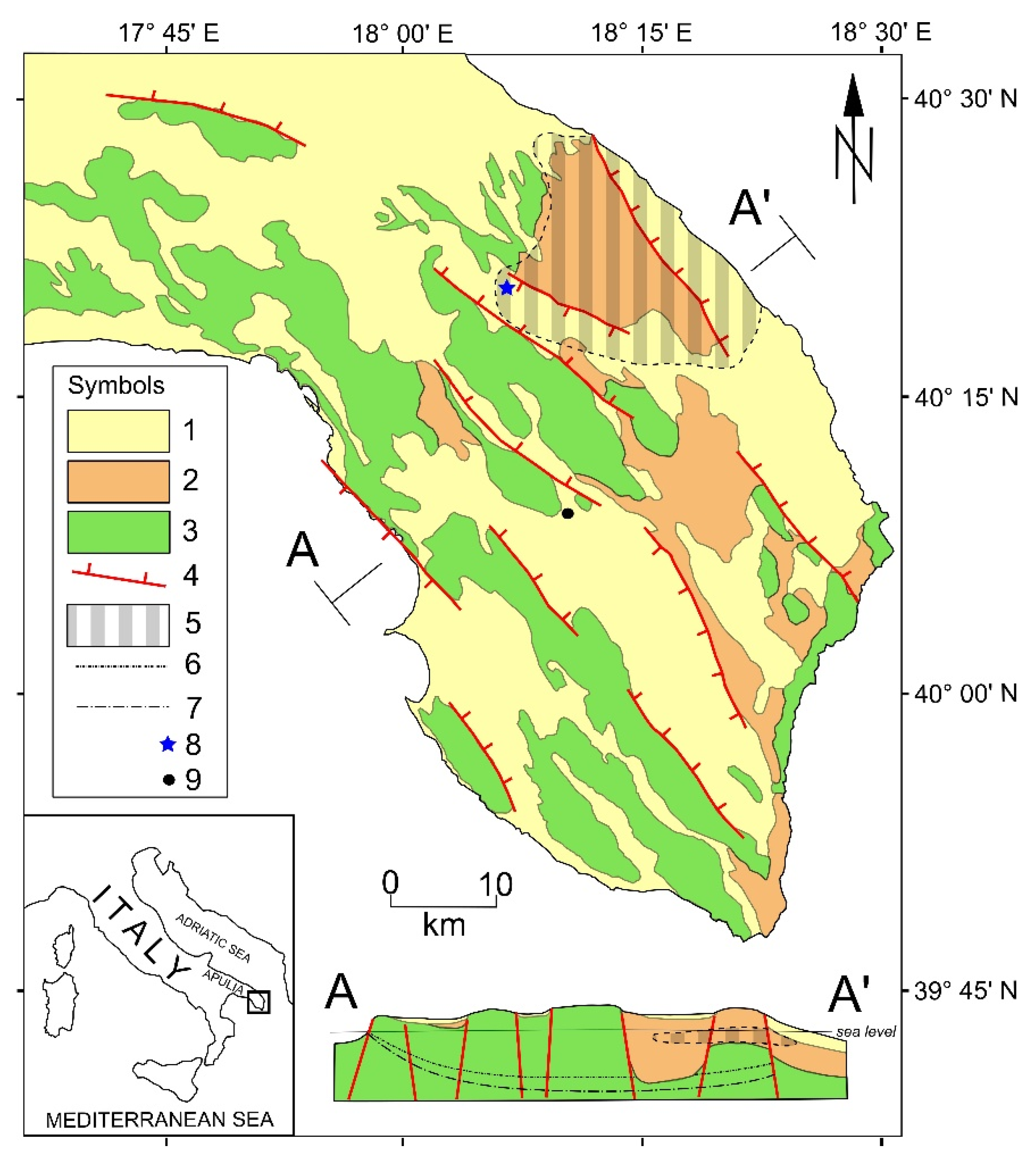
Figure 2.
Ecotekne Campus measurement site. FW, Fiorini Well; BW, Benessere Well; IMS, ISAC-CNR micrometeorological station. In the left side, the hydrostratigraphy of FW is reported (A, upper part of the vadose zone; B, lower part of the vadose zone; C, local shallow aquifer). After [10], modified.
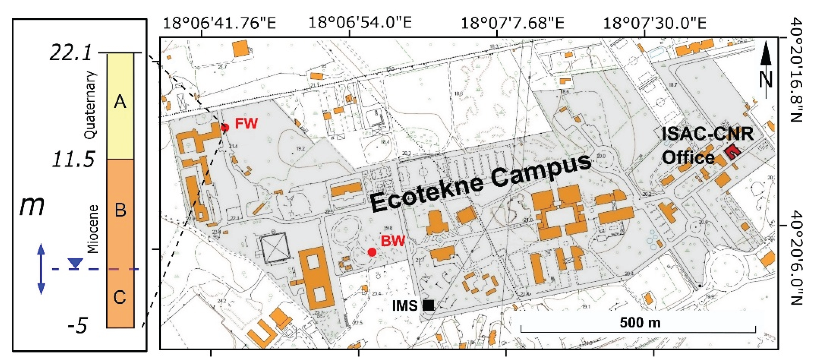
Figure 3.
First interpretation of possible phase delay between water table peaks and atmospheric pressure peaks. PTL, Peak time lag. The dashed line is intended only to aid viewing.
Figure 3.
First interpretation of possible phase delay between water table peaks and atmospheric pressure peaks. PTL, Peak time lag. The dashed line is intended only to aid viewing.
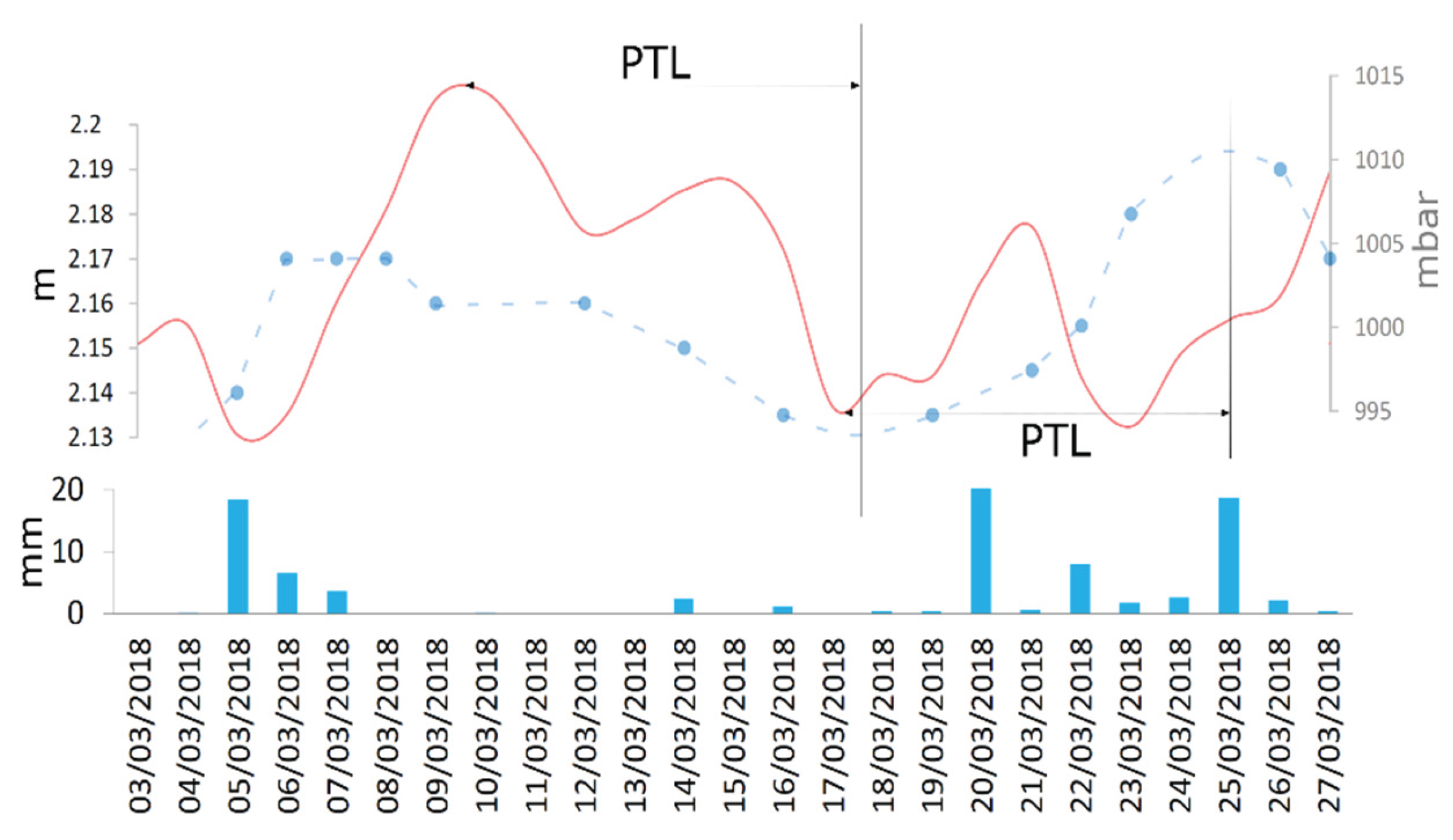
Figure 4.
Comparison between FW level, daily average atmospheric pressure, and daily rainfall.
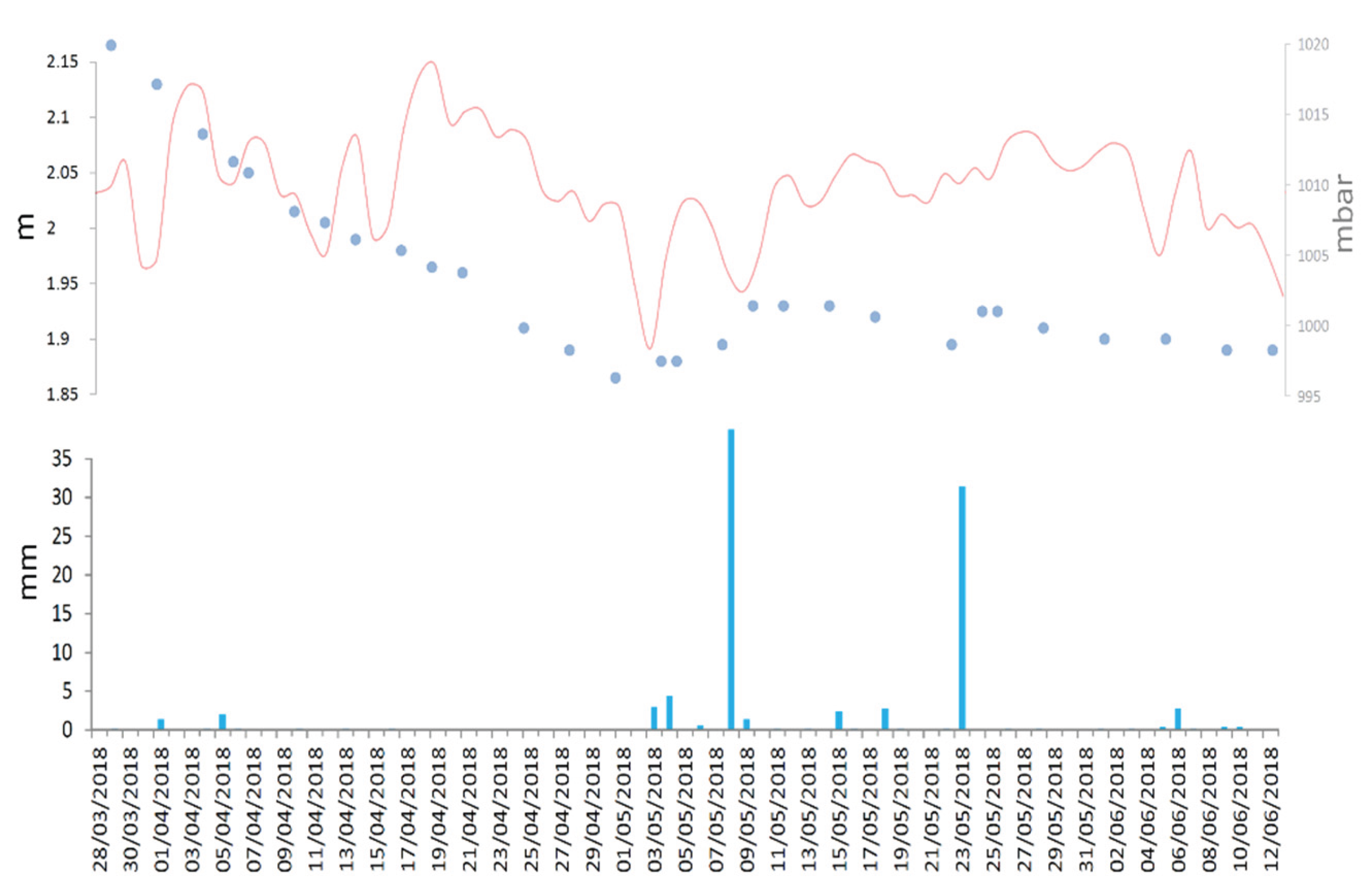
Figure 5.
Comparison between WTFs in the monitoring wells since June 2018 until March 2019. Smooth continuous lines (top side); difference in water table elevation (bottom side). Asterisks mark the day of severe weather conditions (more than 20 mm/day of rain).
Figure 5.
Comparison between WTFs in the monitoring wells since June 2018 until March 2019. Smooth continuous lines (top side); difference in water table elevation (bottom side). Asterisks mark the day of severe weather conditions (more than 20 mm/day of rain).
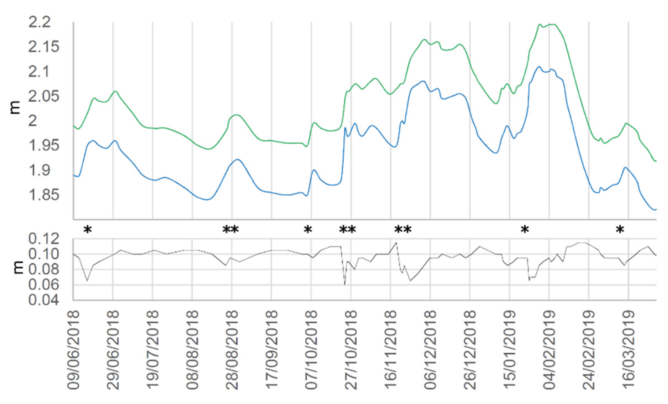
Figure 6.
Comparison between FW (blue points) and BW (green points) levels (in m a.s.l.), daily average atmospheric pressure (in mbar), and daily rainfall (in mm) from 26 December 2023 to 1 March 2024. PTL, Peak time lag between water table peaks and atmospheric pressure peaks.
Figure 6.
Comparison between FW (blue points) and BW (green points) levels (in m a.s.l.), daily average atmospheric pressure (in mbar), and daily rainfall (in mm) from 26 December 2023 to 1 March 2024. PTL, Peak time lag between water table peaks and atmospheric pressure peaks.
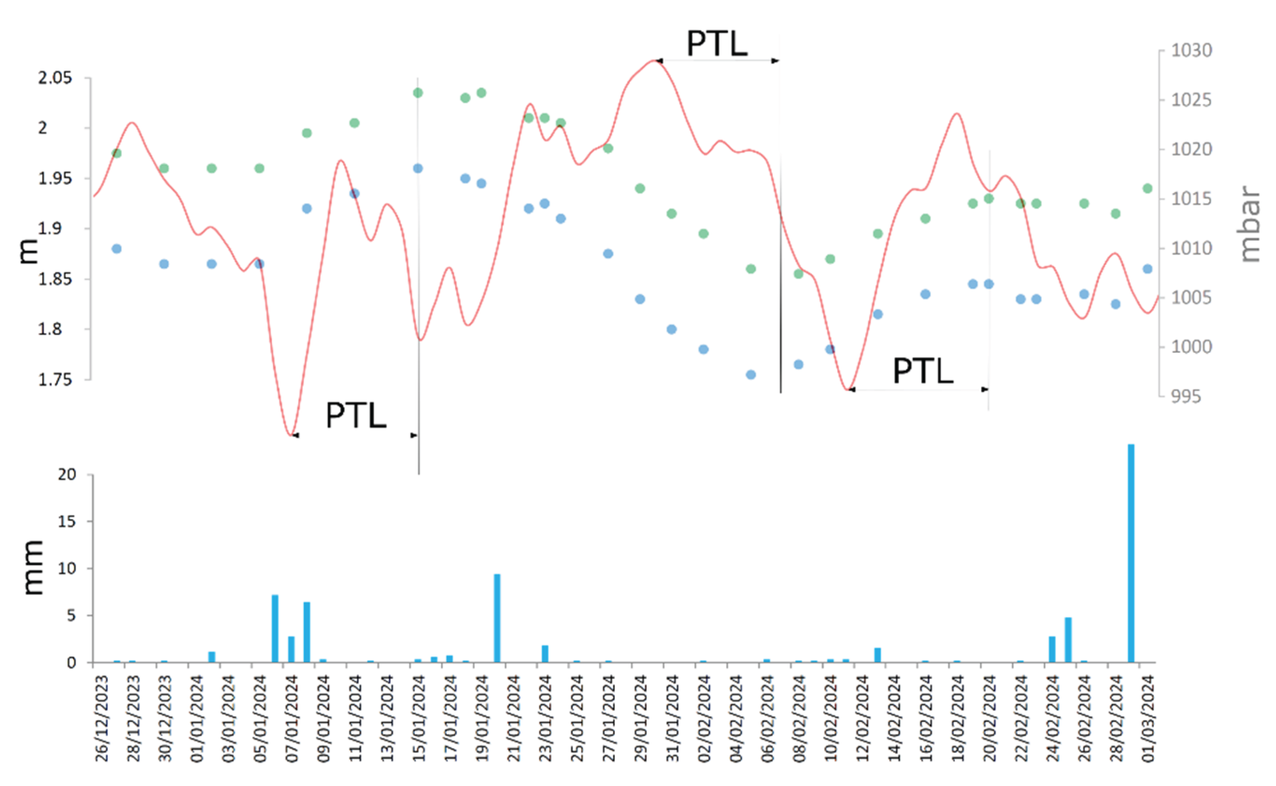
Figure 7.
Comparison between FW (blue points) and BW (green points) levels (in m a.s.l.), daily average atmospheric pressure (in mbar), and daily rainfall (in mm) from 28 December 2024 to 20 March 2025. PTL, Peak time lag between water table peaks and atmospheric pressure peaks.
Figure 7.
Comparison between FW (blue points) and BW (green points) levels (in m a.s.l.), daily average atmospheric pressure (in mbar), and daily rainfall (in mm) from 28 December 2024 to 20 March 2025. PTL, Peak time lag between water table peaks and atmospheric pressure peaks.
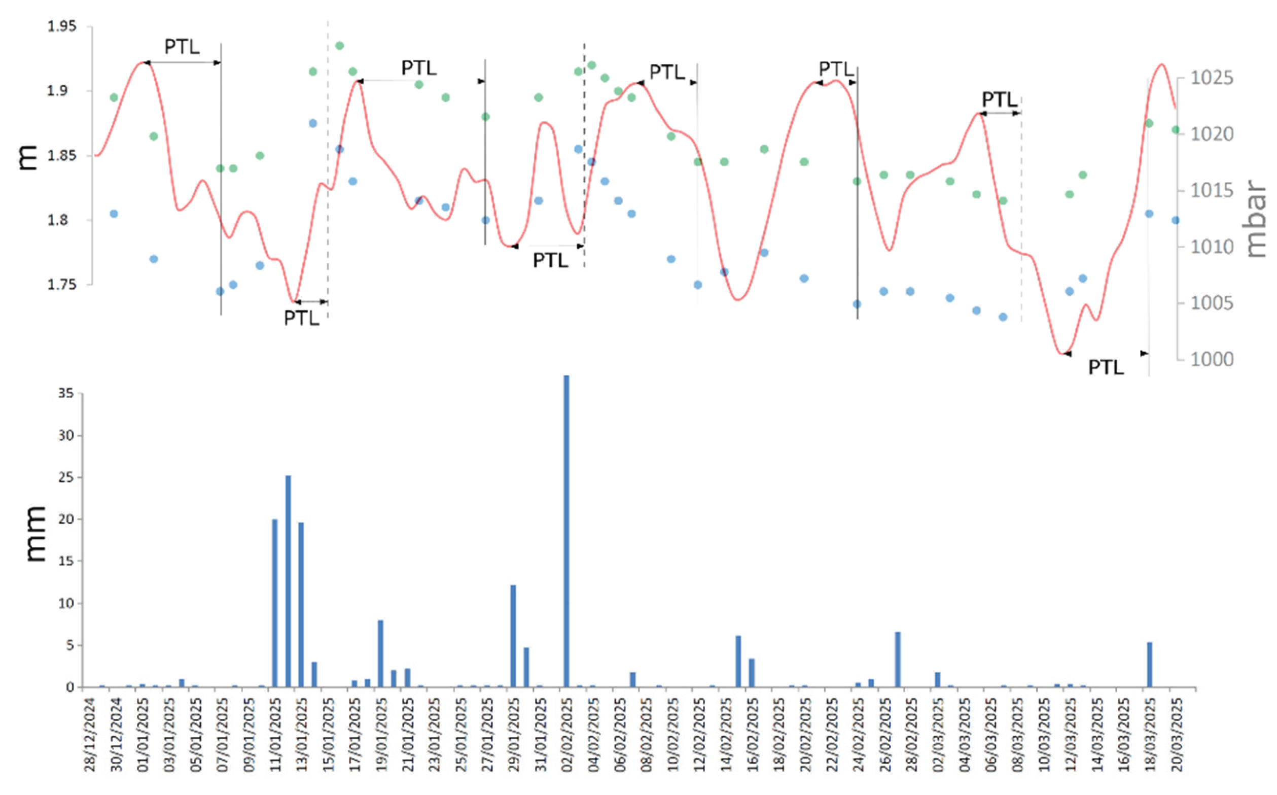
Figure 8.
FW level (in m a.s.l.) recorded during 2017-2018; the 4th order polynomial trend line is reported to aid viewing (black line). Below, monthly rainfall histogram.
Figure 8.
FW level (in m a.s.l.) recorded during 2017-2018; the 4th order polynomial trend line is reported to aid viewing (black line). Below, monthly rainfall histogram.
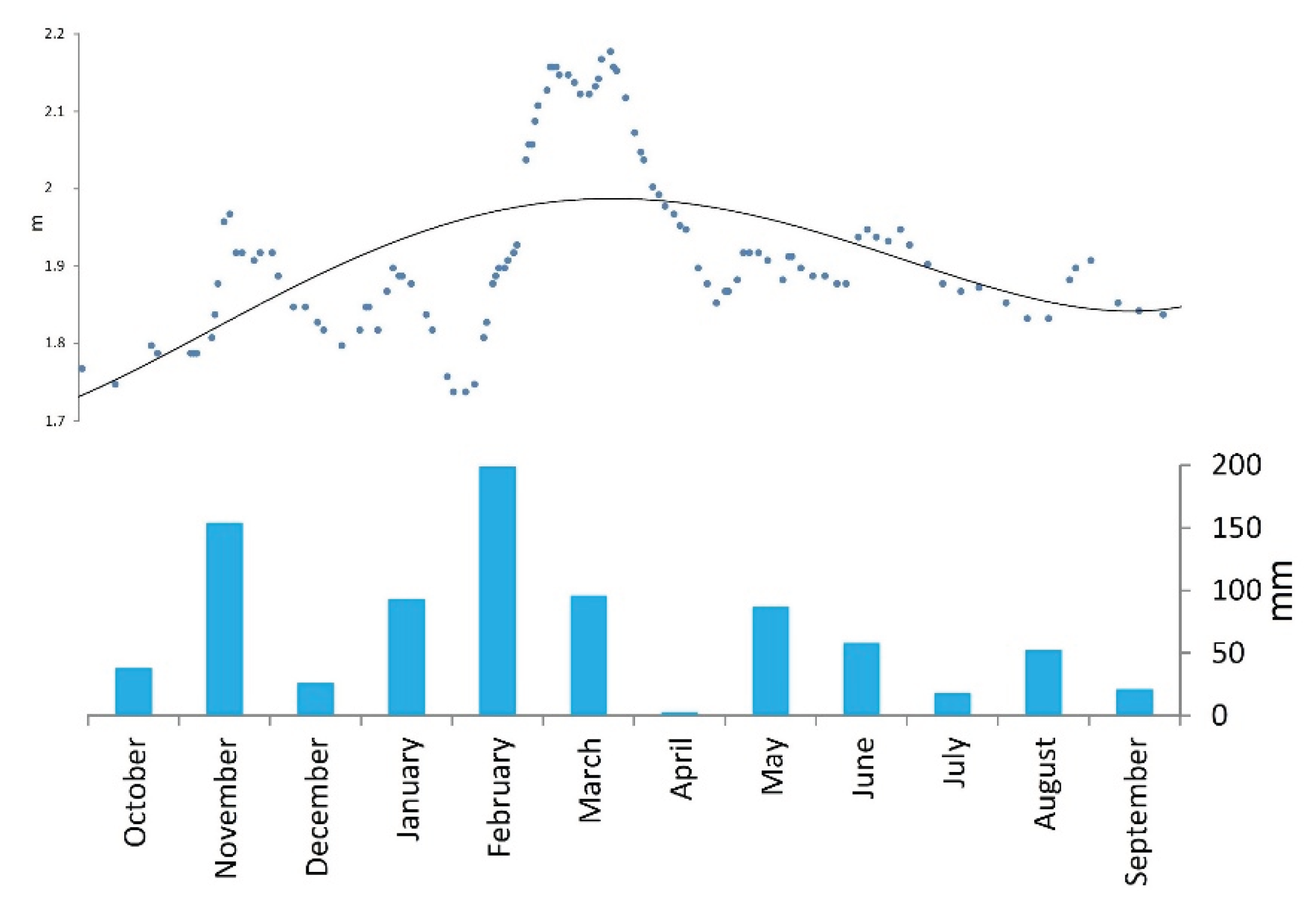
Figure 9.
FW level (in m a.s.l.) recorded during 2023-2024; the 3rd order polynomial trend line is reported to aid viewing (black line). Below, monthly rainfall histogram,.
Figure 9.
FW level (in m a.s.l.) recorded during 2023-2024; the 3rd order polynomial trend line is reported to aid viewing (black line). Below, monthly rainfall histogram,.
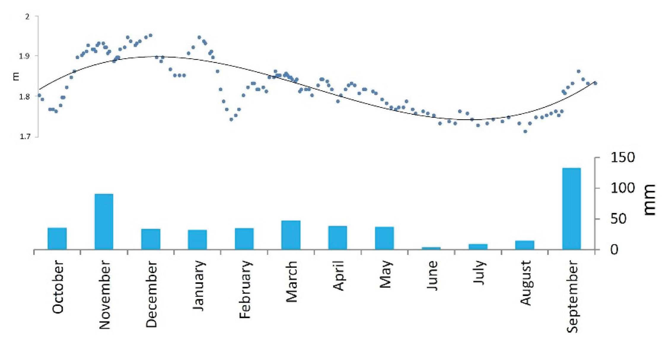
Figure 10.
Smoothed FW hydrographs (level in m a.s.l.) with linear regression (red line) and 4th order polynomial trend (black line).
Figure 10.
Smoothed FW hydrographs (level in m a.s.l.) with linear regression (red line) and 4th order polynomial trend (black line).
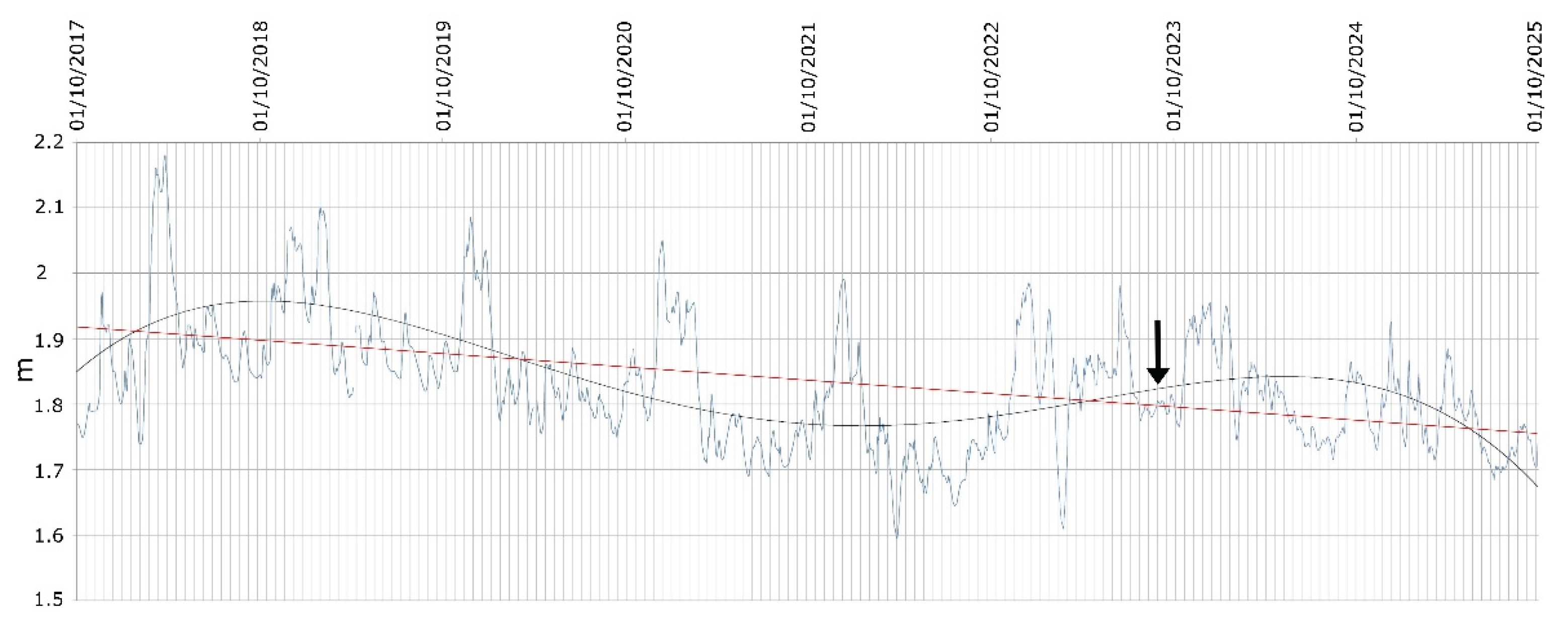
Figure 11.
Scatter diagram of annual precipitation variation (APV, in mm) versus annual groundwater level change (AGLC, in m) calculated for FW.
Figure 11.
Scatter diagram of annual precipitation variation (APV, in mm) versus annual groundwater level change (AGLC, in m) calculated for FW.
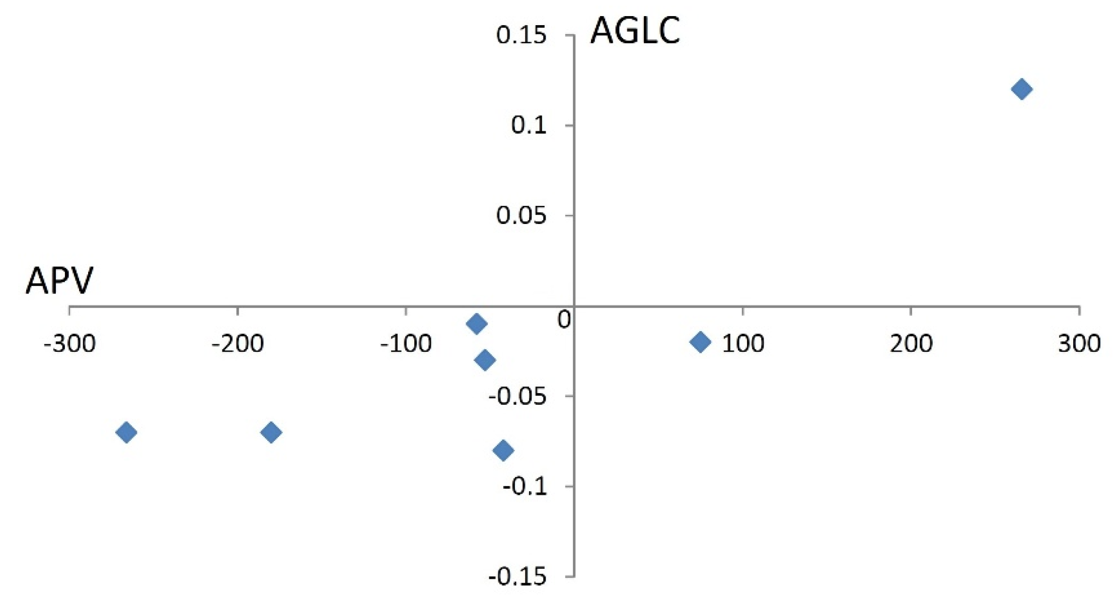
Figure 12.
Dark line, Vora Bosco hydrograph (redrawn from Figure 6 of Ref. [68]); blue line, smoothed FW hydrograph (see text).
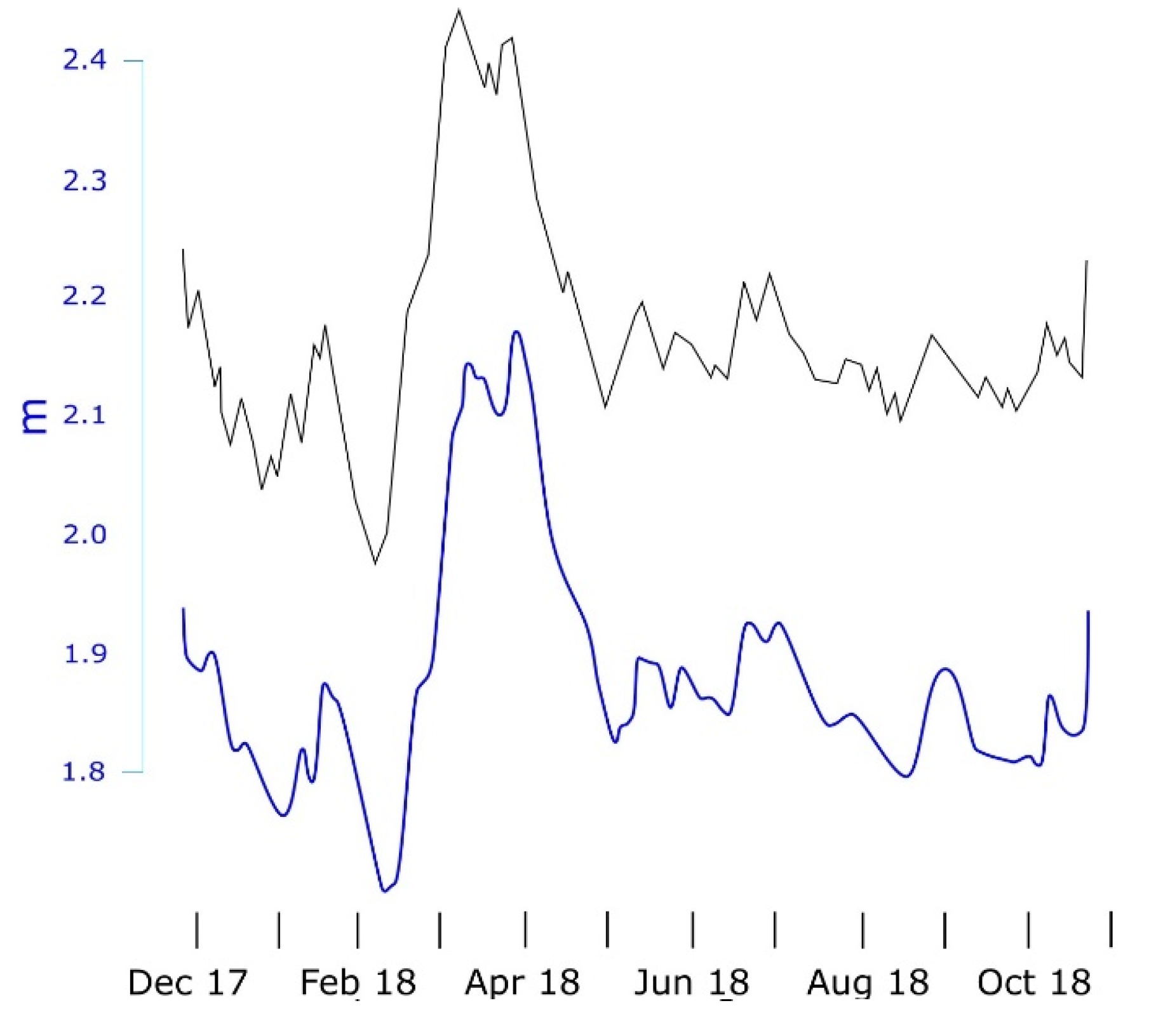

Table 1.
Highest level in the rainy season (in m a.s.l), lowest level in the dry season (in m a.s.l), and annual difference between the levels (in m) recorded in FW during 2017-2025 hydrological years.
Table 1.
Highest level in the rainy season (in m a.s.l), lowest level in the dry season (in m a.s.l), and annual difference between the levels (in m) recorded in FW during 2017-2025 hydrological years.
| Hydrological Year | Highest Rainy Season Level | Lowest Dry Season Level | Annual difference |
| 2017-2018 | 2.16 | 1.82 | 0.34 |
| 2018-2019 | 2.09 | 1.81 | 0.28 |
| 2019-2020 | 2.07 | 1.74 | 0.33 |
| 2020-2021 | 2.03 | 1.68 | 0.35 |
| 2021-2022 | 1.97 | 1.64 | 0.33 |
| 2022-2023 | 1.96 | 1.77 | 0.19 |
| 2023-2024 | 1.93 | 1.7 | 0.23 |
| 2024-2025 | 1.92 | 1.67 | 0.25 |
Table 2.
Cumulative annual precipitation (in mm), annual precipitation variation (in mm), annual groundwater level change (in m).
Table 2.
Cumulative annual precipitation (in mm), annual precipitation variation (in mm), annual groundwater level change (in m).
| Fiorini Well | Benessere Well | |||
| Hydrological Year | Annual Precipitation | APV | AGLC1 | AGLC 1 |
| 2017-2018 | 845 | |||
| 2018-2019 | 787 | -58 | -0.01 | -0.01 |
| 2019-2020 | 607 | -180 | -0.07 | -0.08 |
| 2020-2021 | 565 | -42 | -0.08 | -0.07 |
| 2021-2022 | 512 | -53 | -0.03 | -0.03 |
| 2022-2023 | 778 | +266 | +0.12 | +0.12 |
| 2023-2024 | 512 | -266 | -0.07 | -0.08 |
| 2024-2025 | 587 | +75 | -0.02 | -0.02 |
1 inter-annual difference between the averages of the water table levels measured in the drought July-August period (see text).
Disclaimer/Publisher’s Note: The statements, opinions and data contained in all publications are solely those of the individual author(s) and contributor(s) and not of MDPI and/or the editor(s). MDPI and/or the editor(s) disclaim responsibility for any injury to people or property resulting from any ideas, methods, instructions or products referred to in the content. |
© 2025 by the authors. Licensee MDPI, Basel, Switzerland. This article is an open access article distributed under the terms and conditions of the Creative Commons Attribution (CC BY) license (http://creativecommons.org/licenses/by/4.0/).
Copyright: This open access article is published under a Creative Commons CC BY 4.0 license, which permit the free download, distribution, and reuse, provided that the author and preprint are cited in any reuse.


