Annual Rainfall Forecasting Using Artificial Neural Networks with Stochastic Modeling Approach

S. M. Karthik; M. Gunasekaran; M. Hilaria Soundari; A. Balakrishnan

doi:10.20944/preprints202510.0184.v1

Submitted:

01 October 2025

Posted:

02 October 2025

You are already at the latest version

Abstract

India remains an agrarian society, with agriculture contributing around 13.7% to the national GDP and employing nearly 50% of the workforce. Rainfall plays a pivotal role in sustaining agriculture by irrigating fields and replenishing rivers as well as groundwater reserves. Consequently, understanding rainfall patterns is vital for the country’s economic growth and overall welfare. Accurate rainfall forecasting not only supports better agricultural planning but also aids in flood management and disaster preparedness. Artificial Neural Networks (ANNs) provide a promising approach for predicting monthly rainfall by capturing the cyclical nature of weather systems. This technique utilizes historical time-series data, making it less sensitive to shifts in underlying climate models, including anthropogenic climate change. In this study, ANNs are applied to forecast monthly rainfall, where rainfall data for each of the twelve months is used to predict values for the subsequent year. The neural network is trained using the gradient descent algorithm, and its performance is assessed through four key metrics: Mean Squared Error (MSE), Root Mean Squared Error (RMSE), Mean Absolute Deviation (MAD), and Mean Absolute Percentage Error (MAPE). Experimental results indicate that ANNs can effectively forecast monthly rainfall trends for the period 2025 to 2030.

Keywords:

stochastic modeling

;

ANN

;

annual rainfall

;

prediction

;

flood prevention

Subject:

Computer Science and Mathematics - Mathematics

I. Introduction

Rainfall plays a crucial role in the Indian economy. Approximately 50% of India’s vast labor force relies primarily on agriculture [1,2,3,4]. A significant portion of agricultural activities is directly or indirectly influenced by rainfall. In India, rainfall patterns are highly unpredictable, varying by region and year. The average annual precipitation is around 125 cm. The majority of this rainfall occurs from June to September, a period referred to as the monsoon season. Monsoon winds transport moisture from the Arabian Sea and the Bay of Bengal, resulting in rainfall over the Indian plateau. According to records from the Meteorological department, Cherrapunji in Meghalaya is the wettest area in Asia, receiving approximately 1000 cm of rainfall. In June, rising temperatures in northern India create a low-pressure area, which is filled by winds from the oceans [5,6]. These moisture-laden winds are captured by the Himalayan range, leading to precipitation in the plains of India. The southwest monsoon in June and the northeast monsoon in September represent two distinct systems that bring rainfall to India [7].

The monsoons are essential to the Indian economy. Favorable monsoon conditions result in improved agricultural yields, which enhance rural consumption and create job opportunities. About half of India’s growing population depends on agriculture and related sectors. Positive forecasts of monsoon rains often correlate with rising stock market indices in Mumbai. Besides irrigating farmland, rainfall also helps replenish groundwater supplies. India’s groundwater resources are under significant strain due to a rising population. Numerous deep wells are spread throughout the rural landscape, while rainwater harvesting techniques are just starting to gain traction. This underscores the importance of annual rainfall [8].

Another important aspect of rainfall forecasting is flood management. The urban infrastructure was not equipped to manage sudden flash floods, which caused major disruptions in what is regarded as the financial hub of India. Similar situations have been observed in Chennai in recent years. Accurate predictions of forthcoming rainfall can significantly aid in managing flood scenarios, especially in large, overcrowded cities [9].

II. Study Area and Data

The area-weighted monthly and annual precipitation data is sourced from the data.gov.in website, provided by the Indian Ministry of Earth Sciences. The cumulative annual rainfall in India spans from 1901 to 2024 [10]. The peak rainfall recorded was 1463.9 mm in 1917, while the lowest was 947.1 mm in 1972. In general, the total rainfall does not exhibit a specific pattern. Nevertheless, it is highly unpredictable with alternating periods of drought and rainfall, stemming from a chaotic weather system [11]. Figure 1 presents a box plot illustrating the monthly fluctuations in rainfall. The period from June to October constitutes the monsoon season, characterized by both significant amounts and variability in rainfall. July records the highest rainfall levels and shows the greatest variability. In contrast, the other months receive less than 75 mm of rain and display less unpredictability. Figure 2 further illustrates the monthly variations in rainfall.

Figure 3 illustrates the examination of the relationship between rainfall patterns over several years. The box plot categorizes the data into three groups: the first group represents the correlation between the rainfall patterns of the first year and the second year, the second group pertains to the correlation between the patterns of the first year and the third year, and the third group relates to the correlation between the patterns of the first year and the fourth year. The correlations observed between consecutive years exhibit the strongest correlation, with most values exceeding 0.91. The outliers in this analysis are the years 1905, 1953, and 2004, which have correlations of 0.87, 0.88, and 0.89, respectively. These years do not show improved correlation with any other years. This indicates that the most accurate predictions can be made by utilizing the rainfall data from one year to forecast the following year’s patterns.

III. Artificial Neural Network (ANN)

The Artificial Neural Network (ANN) approach was introduced by Hamzacebi in [12,13,14]. This method is adept at learning and predicting nonlinear relationships in time series data. In contrast to Autoregressive Integrated Moving Average (ARIMA) [15,16] models, ANN retains variations in the data. It identifies patterns and accurately forecasts future values in the time series [17,18]. Empirical evidence has shown that it performs exceptionally well in domains like weather prediction and stock market analysis[19]. In these scenarios, the variables being measured often exhibit various cyclical patterns with distinct time periods and phase shifts. The Artificial Neural Network (ANN) [20,21,22] operates as a supervised learning mechanism and is capable of modeling nonlinear relationships[23,24,25]. The input layer of the ANN consists of s nodes, with s representing the variation period. For monthly rainfall data, s is set to 12, aligning with the twelve months of the year. Data for each month is inputted through the neurons in this layer. STORAGE functions as a temporal stochastic simulator, developed to produce extended and high-resolution rainfall time series[26]. The Markov chain method used to predict the precipitation on short period, the prediction performance of Markov chain model is related with the forecasting steps [27,28].

A hidden layer is also included, containing a specific number of neurons. The greater the number of neurons in the hidden layer, the more complex and effective the ANN’s modeling capabilities become. However, if there are too many hidden neurons, the training data may be inadequate. In our tests, we utilize 6 neurons in the hidden layer. The output layer is designed to forecast the monthly rainfall for the subsequent year. Figure 4 provides a visualization of the ANN utilized in this study.

Let

R_{i, j}

be the amount of rainfall observed in the jth month of the ith year. The input neurons are fed with

R_{i, j}, j = 1,2, \dots, 12 .

The output neurons are trained to give

R_{i + 1, j}, j = 1,2, \dots, 12

. The weights

U_{j, k}, j = 1,2, \dots, 12; k = 1,2, . . ., h

are present in the connections between the 12 neurons in the input layer and the h neurons in the hidden layer. The weights

V_{k, j}, j = 1,2, \dots, 12; k = 1,2, . . ., h

are present in the connections between the h neurons in the hidden layer and the 12 nodes in the output layer. In addition to these neurons, bias neurons with the weights

α_{k}

and

β_{j}

are present. The relationship between the output and input neurons are captured by the equation.

{\hat{R}}_{i + 1, j} = β_{j} + \sum_{k = 1}^{h} (V_{k j} f (α_{k} + \sum_{j = 1}^{12} U_{j, k} R_{i, j}))

(1)

Here f is the activation function. The choice of a proper architecture is crucial in the accuracy of all types of ANNs. The only parameter here is h which the number of neurons in the hidden layer is. It is decided on an empirical basis. Common activation functions used include logistic function, softmax function and the gaussian function. In this work, the gaussian function is used because the predicted variable is continuous.

The data consists of 126 years of observations. It is partitioned randomly into training and testing set each consisting of 57 observations. The parameter h is varied from 4 to 9. The gradient descent method is used for training. The experimental results are summarized in the next section.

IV. Experimental Results and Analysis

I. Performance Measures

Let

R_{i, j}, i = 1,2, . ., n; j = 1,2, \dots, 12

be the actual rainfall recorded in the test set for n years. Let

{\hat{R}}_{i, j}

be the prediction for the same period from the ANN. Then the following performance measures are used to assess the accuracy of the prediction.

Mean Squared Error (MSE) is defined as

m s e = \frac{1}{12 n} \sum_{i = 1}^{n} \sum_{j = 1}^{12} {(R_{i, j} - {\hat{R}}_{i, j})}^{2}

(2)

Root Mean Squared Error (RMSE) is defined as

r m s e = \sqrt{m s e}

(3)

Mean Absolute Deviation (MAD) is defined as

m a d = \frac{1}{12 n} \sum_{i = 1}^{n} \sum_{j = 1}^{12} |R_{i, j} - {\hat{R}}_{i, j}|

(4)

It is the average of all absolute deviations of the predicted from the actual values.

Mean Absolute Prediction Error (MAPE) [8] is also known as Mean Absolute Percentage Deviation (MAPD). It is defined as

m a p e = \frac{1}{12 n} \sum_{i = 1}^{n} \sum_{j = 1}^{12} |\frac{R_{i, j} - {\hat{R}}_{i, j}}{R_{i, j}}|

(5)

MAPE can be used in our current application since there are no zero values in the predicted variable and does not cause division by zero error. When MAPE is multiplied by 100, it is expressed as a percentage. MSE, RMSE, MAD and MAPE must be low for a good prediction. RMSE, MAD and MAPE are expressed in the same units as the predicted variable i.e., in mm in this case.

II. Neural Network Training and Results

The ANN was trained with number of neurons in the hidden layer ranging from 4 to 9. Figure 5 shows the training parameters with the MATLAB Neural Network Toolbox. The results are summarized in Figure 6, Figure 7, Figure 8, Figure 9, Figure 10 and Figure 11. The prediction values are plotted against the actual values for one representative year out of the 57 years (i.e., 12 months) in the test set.

I. Performance Analysis in ANN

The summary of the performance analysis is presented in Table 1. It provides the values for MSE, RMSE, MAD, and MAPE for the parameter h, which varies from 4 to 12.

Based on the performance metrics, increasing the number of neurons in the hidden layer leads to improved accuracy. A larger number of neurons in the hidden layer allows for capturing more intricate relationships within the time series data. However, after reaching a certain threshold, the improvement in accuracy becomes negligible. Table 1 indicates that there is only a slight enhancement when the number of hidden neurons exceeds 7. The best performance is achieved with 8 hidden neurons. The RMSE of 8.77 indicates that rainfall predictions can be expected to have an average error margin of ± 6 mm. For h = 8, the MAPE is approximately 10%. Thus, rainfall can be forecasted reliably using ANN. The MAD is under 6.00 for h = 8. The highest deviation recorded in the predictions for the test set is 9 mm. A comparative evaluation has been conducted, and the findings are presented in Table 2. The ANN with h = 8 is evaluated alongside Autoregressive Moving Average (ARMA) [9], Autoregressive Integrated Moving Average (ARIMA), Seasonal Autoregressive Integrated Moving Average (SARIMA) [10], and Hidden Markov Models (HMM) [11]. The ANN outperforms the HMMs, achieving the highest performance.

II. Annual Rainfall Prediction 2025 to 20230

The ANN model is utilized to forecast rainfall from 2025 to 2030. The findings are presented in summary form below. Figure 10 illustrates the projected average annual rainfall for those years. Figure 11 depicts the anticipated monthly rainfall for the same timeframe.

Figure 10. Average Annual Rainfall forecasted 2025 to 2030.

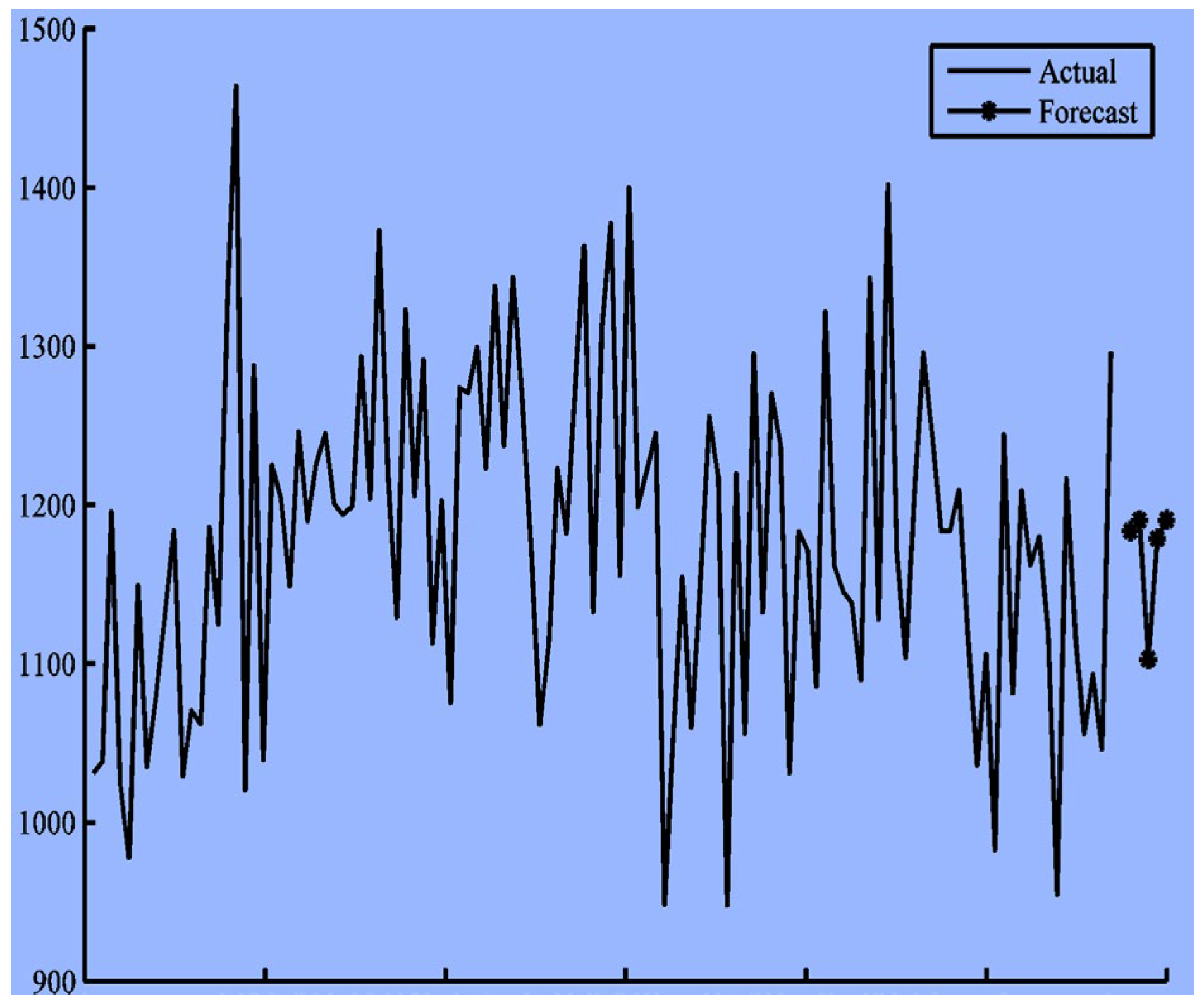
Figure 11. Monthly Rainfall forecasted for 2025 to 2030 (60 months).

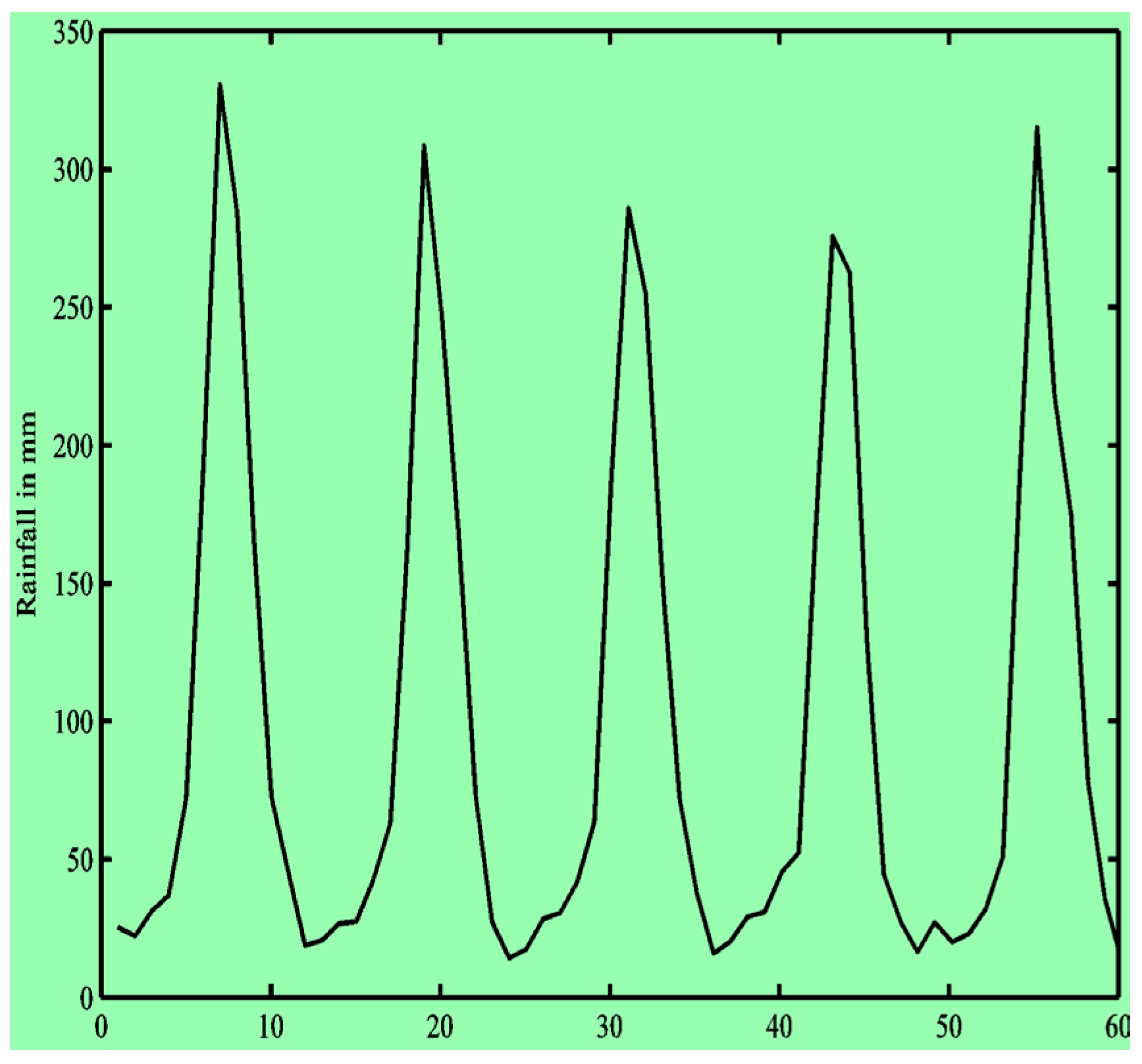
The accuracy of forecasts for extended periods tends to be low due to the compounding errors in the predictions. Nonetheless, it is typical for chaotic systems, such as weather patterns, to show decreasing reliability in longer-term predictions. Still, it is possible to forecast the entire upcoming year, which can be useful for planning agricultural activities and managing floods.

V. Conclusion

Prediction rainfall is a crucial element of weather management. This study focused on predicting rainfall using an artificial neural network (ANN). The data’s characteristics are effectively captured through the ANN framework. A brief explanation of the ANN concept and its mathematical models was provided. Experiments were conducted using monthly rainfall data covering the years 1901 to 2024. The statistical properties of the data were illustrated through visualization techniques. Performance metrics suggest that the predictions are dependable within an error margin of ±6 mm. This level of accuracy is beneficial for agricultural planning and flood management. Forecasts for rainfall up to 2020 are included in this study. The results are compared with common forecasting methods like ARMA, ARIMA, SARIMA, and HMMs, demonstrating the superior accuracy of the ANN approach. Future research could explore integrating the high accuracy of ANN with the stability offered by HMMs for longer-term forecasting. Additionally, predictions could be broadened to include other variables such as surface temperature, humidity, and cyclones.

References

Harris, L. , McRae, A. T. T., Chantry, M., Dueben, P. D., & Palmer, T. N. (2022). A generative deep learning approach to stochastic downscaling of precipitation forecasts. N. ( 14, e2022MS003120. [CrossRef]
Skarlatos, K. , Bekri, E. S., Georgakellos, D., Economou, P., & Bersimis, S. (2023). Projecting annual rainfall timeseries using machine learning techniques. Energies, 16. [CrossRef]
Allawi, M. F. , Abdulhameed, U. H. et. al.. (2023). Monthly rainfall forecasting modelling based on advanced machine-learning methods: Tropical region as case study. Engineering Applications of Computational Fluid Mechanics, 17, 2243. [Google Scholar] [CrossRef]
Lathika, P. , & Sheeba Singh, D. (2023). A novel model for rainfall prediction using hybrid stochastic-based Bayesian optimization algorithm. Environmental Science and Pollution Research, 30. [CrossRef]
Sammen, S. S. , Kisi, Ö., Ehteram, M., El-Shafie, A., Al-Ansari, N., Ghorbani, M. A., … Shahid, S. (2023). Rainfall modeling using two different neural networks improved by metaheuristic algorithms. Environmental Sciences Europe, 35. [CrossRef]
[6] Nguyen, T. H. T. , Bennett, B., & Leonard, M. (2023). Evaluating stochastic rainfall models for hydrological modelling. Journal of Hydrology, 627, 3038. [Google Scholar] [CrossRef]
Ríos Gaona, M. F. , Michaelides, K., & Singer, M. B. (2024). STORM v.2: A simple stochastic rainfall model for exploring impacts of climate and climate change at and near the land surface. Geoscientific Model Development, 17. [CrossRef]
Iotti, M. , et al. (2025). RainScaleGAN: conditional generative adversarial network for rainfall downscaling and stochastic generation. Journal of Advances in Modeling Earth Systems / AI in Earth Sciences. [CrossRef]
Wani, O. A. , et al. (2024). Predicting rainfall using machine learning, deep learning, and time-series: a comparative study. Scientific Reports, 14, 1234. [Google Scholar] [CrossRef]
Ji, H. K. , et al. (2024). Implementing generative adversarial networks as a data-driven multi-site stochastic weather generator for flood frequency estimation. Environmental Modelling & Software, 166. [CrossRef]
Ridwan, W. M. , & coauthors. (2021). Rainfall forecasting model using machine learning methods — comparative evaluation. Journal of Atmospheric and Solar-Terrestrial Physics, 224, 0559. [Google Scholar] [CrossRef]
Narejo, S. , et al. (2021). Multi-step rainfall forecasting using deep learning approach. Scientific Reports, 11, 1236. [Google Scholar] [CrossRef]
Farhani, N. , et al. (2022). MetGen: a regional sub-daily stochastic weather generator based on artificial neural networks and statistical components. Environmental Modelling & Software, 157. [CrossRef]
Najibi, N. , et al. (2024). A statewide, weather-regime based stochastic weather generator for California: evaluation and applications. Journal of Hydrology: Regional Studies, 52. [CrossRef]
Northrop, P. J. (2021). Stochastic models of rainfall: review and recent developments. Annual Review of Statistics and Its Application, 8. [CrossRef]
[16.] Behfar, N. [16.] Behfar, N., et al. (2024). Assessing rainfall-runoff models and AI methods for climate change impacts on catchment hydrology. Hydrological Processes, 38, 3236. [Google Scholar] [CrossRef]
Ratha Jeyalakshmi, T & Karthik, S. M. et. al. (2024) “Enhanced Pulmonary Embolism Detection in CT Angiography Using Spectral ResNet Hyper Convolutional Neural Network”, SN Computer Science: A Springer Nature Journal, 5(8),1-14. [CrossRef]
Molina, J. L. , & coauthors. (2025). Bayesian stochastic rainfall generator (BSRG): an intelligent data-driven tool. Water Resources Management, 39. [CrossRef]
Guan, X. , Nguyen, V. D., Voit, P., Merz, B., Heistermann, M., & Vorogushyn, S. (2025). The ability of a stochastic regional weather generator to reproduce heavy-precipitation events across scales. Natural Hazards and Earth System Sciences, 25. [CrossRef]
Zhang, H. , & coauthors. (2020). Semi-empirical LSTM approach for monthly precipitation prediction: a case study. Atmospheric Research, 240. [CrossRef]
He, R. , et al. (2024). Data-driven multi-step prediction and analysis of monthly rainfall using GRU/ANN hybrids. Expert Systems with Applications, 220, 1195. [Google Scholar] [CrossRef]
Bouach, A. , et al. (2024). Improving ANN-based rainfall forecasts with geographically aware postprocessing. Journal of Hydrometeorology, 25, 1362. [Google Scholar] [CrossRef]
Rasool, T. , et al. (2024). Development of a stochastic rainfall generator to yield realistic extreme precipitation events for hydrologic design. Journal of Hydrology, 618, 1286. [Google Scholar] [CrossRef]
Price, I. , et al. (2025). Probabilistic weather forecasting with machine learning: GenCast and beyond. Nature. [CrossRef]
Kothari, A. , et al. (2024). Predicting rainfall using a combined ML/DL/time-series framework: ANN, LSTM, ARIMA comparisons. Scientific Reports, 14, 9876. [Google Scholar] [CrossRef]
De Luca, D. L. , & Petroselli, A. (2021). STORAGE (STOchastic RAinfall GEnerator) v2: updates and ANN conditioning for high-resolution synthetic rainfall sequences. Hydrology, 8. [CrossRef]
Arumugam, P. and Karthik S.M., “Stochastic Modelling in Yearly Rainfall at Tirunelveli District, Tamil Nadu, India”, Journal of Materials Today: Proceedings, Elsevier, 5(1), 1852 – 1858, 2018. [CrossRef]
Karthik. S.M., and Arumugam. P. (2017) “Stochastic modelling based monthly rainfall prediction using seasonal artificial neural networks. “ ICTACT Journal of Soft Computing, 2(2). [CrossRef]

Figure 1. Box Plot of Monthly Variation.

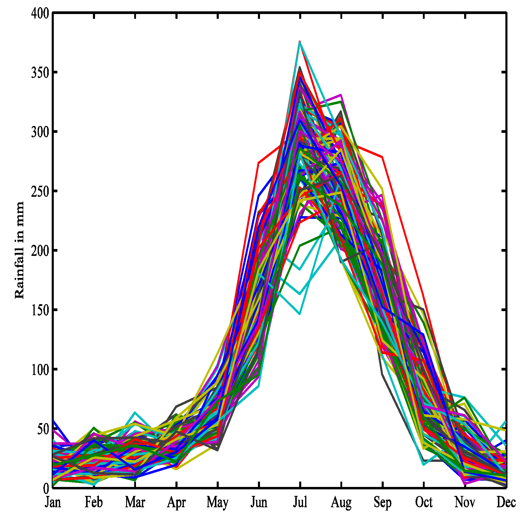
Figure 2. Line Plot of Monthly Variation.

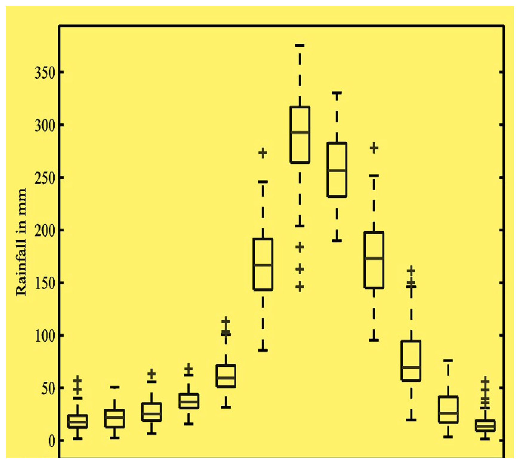
Figure 3. Correlation of Monthly Rainfall with Succeeding Years.

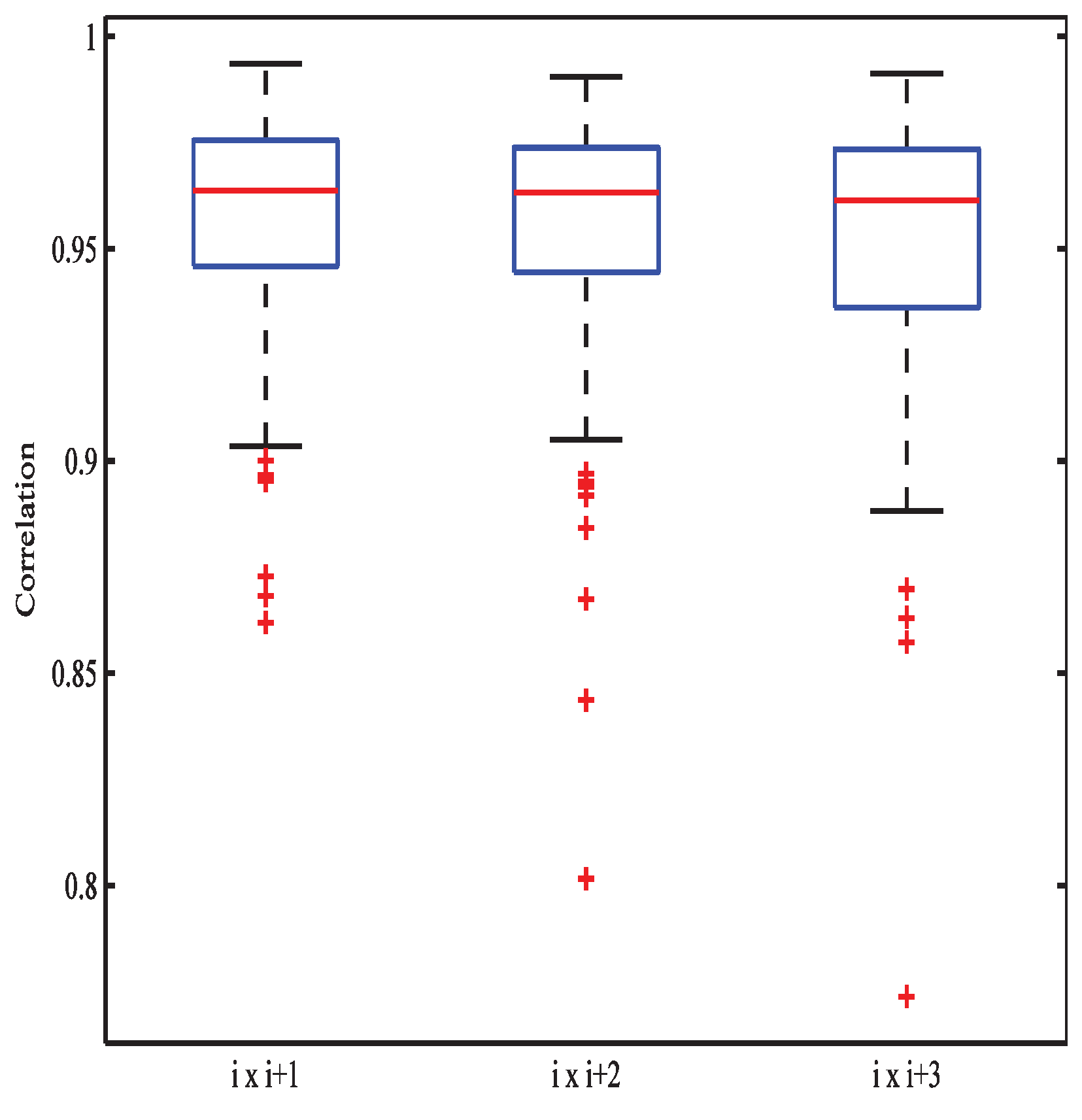
Figure 4. Neural Network with s = 12.

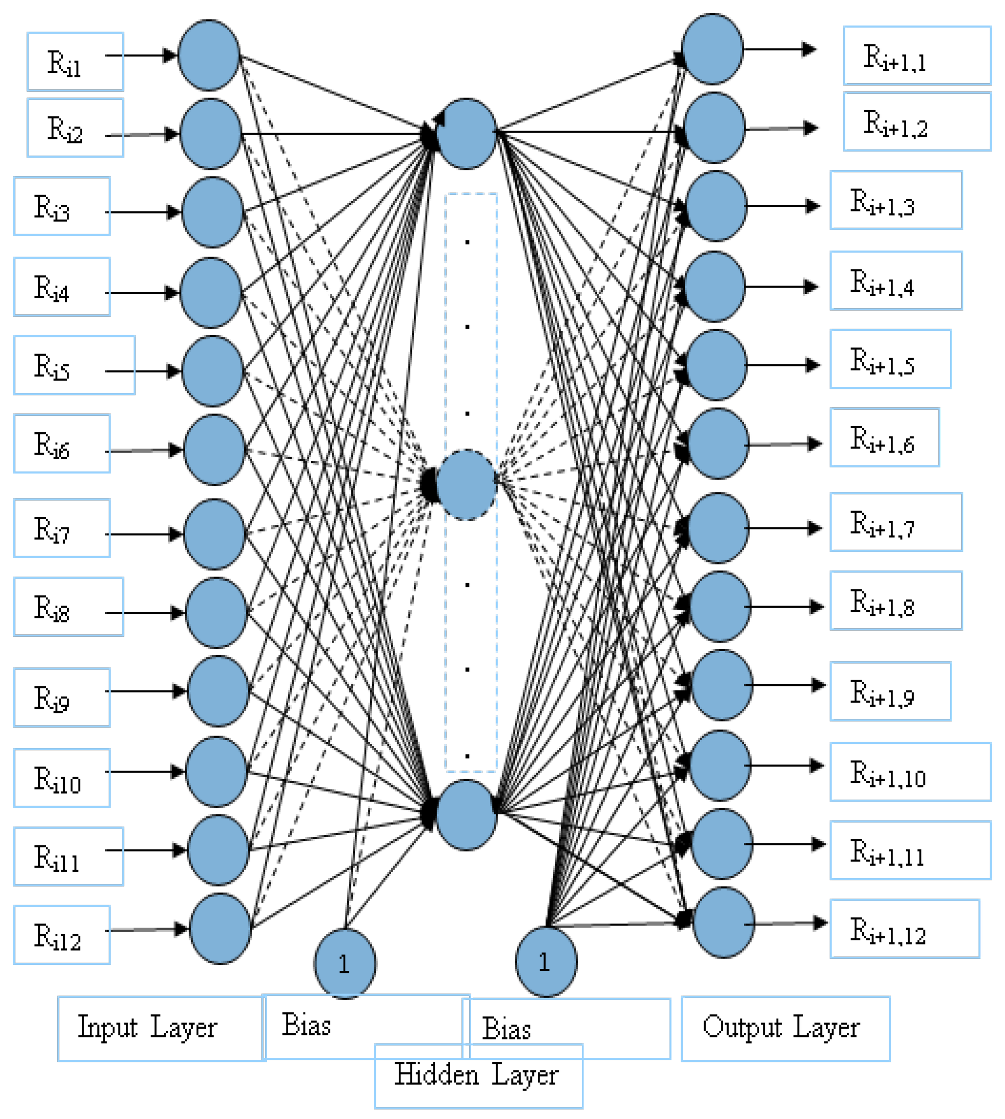
Figure 5. Neural Network Parameters in MATLAB.

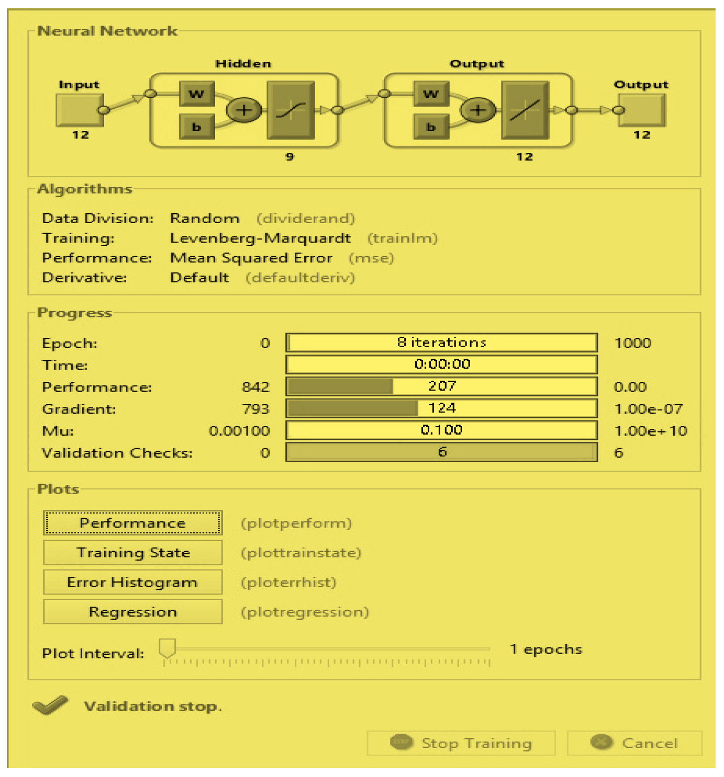
Figure 6. h = 4.

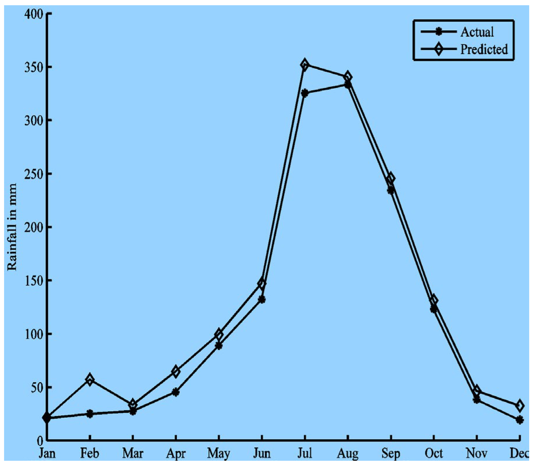
Figure 7. h = 5.

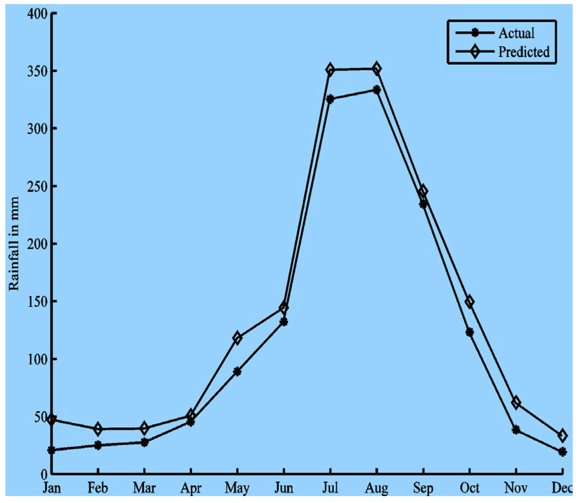
Figure 8. h = 6.

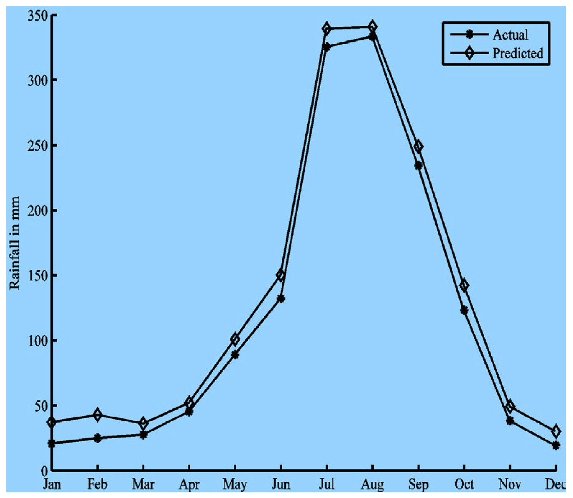
Figure 9. h = 7.

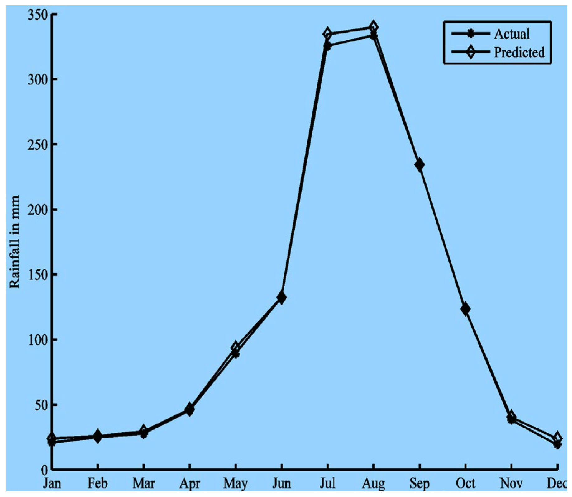
Figure 10. h = 8.

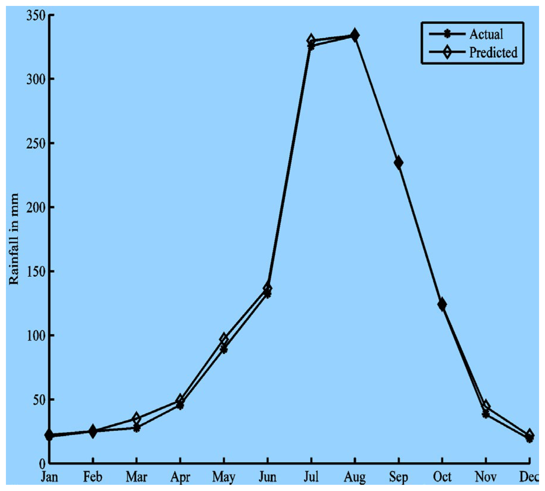
Figure 11. h = 9.

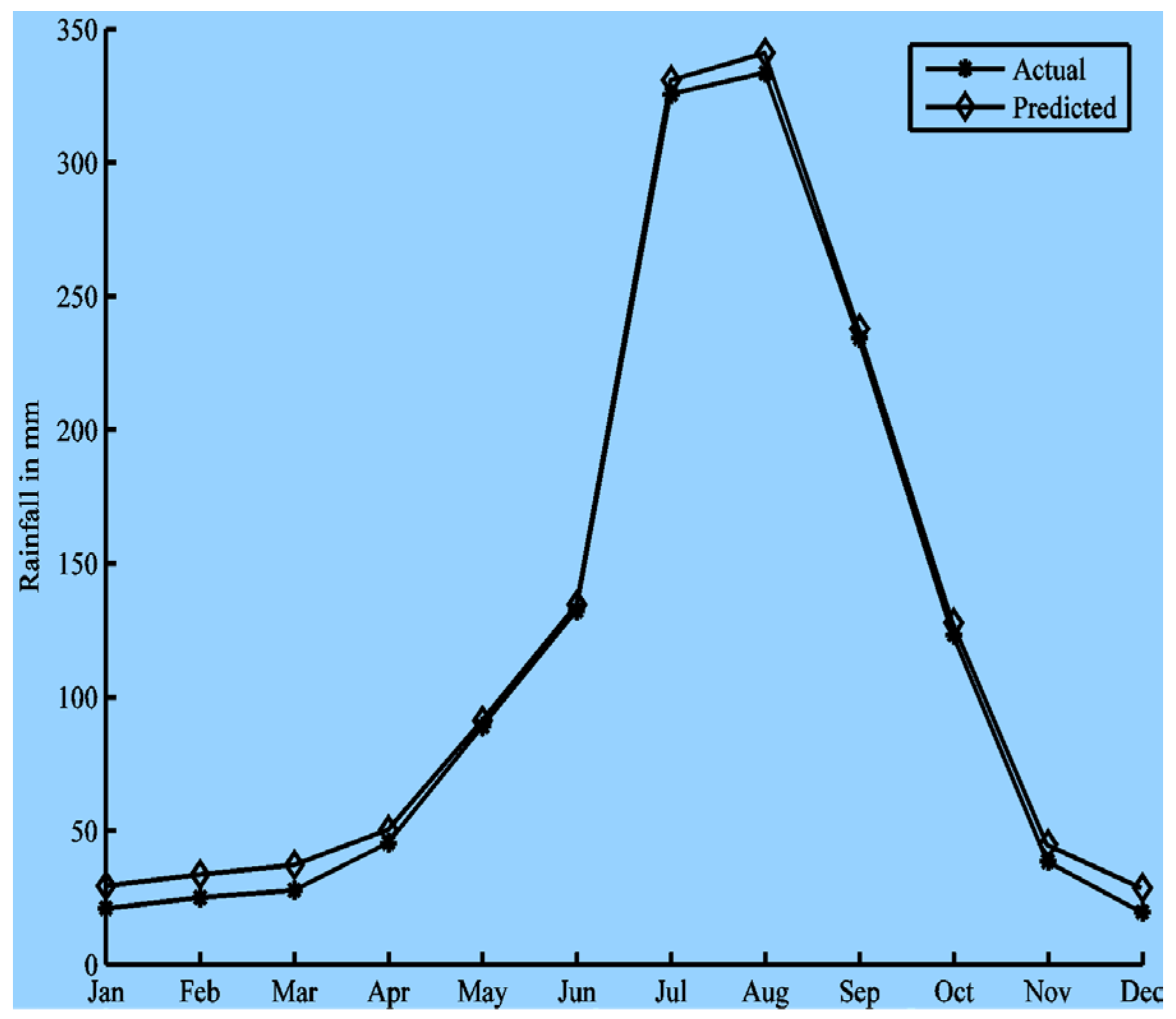
Table 1. Performance Measures for ANN.

h	MSE	RMSE	MAD	MAPE
4	552.10	25.68	22.80	0.53
5	305.85	19.63	17.20	0.42
6	137.58	13.84	12.31	0.42
7	32.78	7.87	6.90	0.30
8	34.69	8.83	6.76	0.31
9	35.52	8.97	8.12	0.34

Table 2. Comparative Analysis.

Method	MSE	RMSE	MAD	MAPE
ANN (h=8)	34.69	7.13	6.86	0.30
HMM	40.68	8.22	7.02	0.32
ARMA	41.40	8.33	7.89	0.33
ARIMA	42.55	8.56	7.33	0.34
SARIMA	45.52	8.44	7.44	0.37

Disclaimer/Publisher’s Note: The statements, opinions and data contained in all publications are solely those of the individual author(s) and contributor(s) and not of MDPI and/or the editor(s). MDPI and/or the editor(s) disclaim responsibility for any injury to people or property resulting from any ideas, methods, instructions or products referred to in the content.

© 2025 by the authors. Licensee MDPI, Basel, Switzerland. This article is an open access article distributed under the terms and conditions of the Creative Commons Attribution (CC BY) license (http://creativecommons.org/licenses/by/4.0/).

Copyright: This open access article is published under a Creative Commons CC BY 4.0 license, which permit the free download, distribution, and reuse, provided that the author and preprint are cited in any reuse.