
Submitted:
23 September 2025
Posted:
24 September 2025
You are already at the latest version
Abstract
This paper reports the preliminary findings of the first initiative of developing a year-round streamflow forecasting system using HBV hydrologic model in a data scarce Ruvu catchment in Tanzania. Considering the importance of the Ruvu catchment as the main source of water to the fast-growing mega city of Dar es Salaam, the researchers in this study made the most of the available data and their joint previous application experience of the modelling framework for the purpose of setting up a reliable operational model. Besides, the researchers adopted a phased approach of developing the streamflow forecasting system, using HBV as hydrological model, which resulted into a simplified model structure with minimized complexity. For instance, the snow routine was removed as it is not relevant to the study area, and a number of parameters was reduced to improve model efficiency. As a measure to improve confidence in model predictions, various error functions were used for hydrological model calibration and validation. Although, Ruvu catchment has been characterized by this study as data scarce catchment, the results of the hydrological forecasting system range from good to very good and varying with season and quality of forecast meteorological data, and the model is already launched for operational use and the forecasts are published online. The authors suggest that any future forecasting initiative should put much emphasis on both the understanding of the modelling framework to be used and adequate data collection and analysis, in a synergetic manner with all relevant agencies. And it is also recommended to be vigilant to changes of the catchment characteristics and model performance during its life cycle as the performance of the developed model is only valid to the condition it was calibrated and validated.
Keywords:
data scarce catchments
; HBV model
; hydrologic modelling
; operational streamflow forecasting system
; Ruvu catchment
; Tanzania
1. Introduction
Hydrological forecasting is a translation of single deterministic or an ensemble of short, intermediate, and long lead-time meteorological forecasts into estimates of hydrological variables of interest (e.g., streamflow, river stage, snowmelt, etc.) via hydrological forecasting models at the corresponding temporal scales [1], [2], [3], [4].
Operational hydrological models are a set of models consisting of more or less interactive routines handling all from validation and correction of input data to finally calculating the runoff forecast or ensemble of such, on short or long term [1], [2], [3], [5], [6]. In an operational environment, it is typically driven by inputs from a wide range of sources, including meteorological observations and forecasts, river observations, and other data types [1], [2].
Hydrological forecasting is of primary importance to better inform decision-making, for instance on flood and drought response strategies, irrigators, reservoir operations, hydropower generation, water resources planning, and environmental flow management [1], [2], [3], [7], [8], [9], [10], [11], [12]. It should be noted that hydrological forecasts possess no “intrinsic value”. They acquire value through their ability to influence the decisions made by users of the forecasts [13], [14].
Hydrological models can be broadly classified into three categories: empirical models (Black box), conceptual models (Grey box), and physically based models (White box), [15]. Conceptual and empirical driven models are usually used in lumped or semi-distributed forms [1], [2]. The Hydrologiska Byrans VattenbalansavdeIning (HBV) is a conceptual hydrological model extensively used in operational hydrological forecasting and water balance studies [16], [17]. As with many other types of models, hydrological forecasting models are subject to many sources of uncertainty, including uncertainties in the input data, model parameters, initial conditions, and boundary conditions [1], [2], [18]. The model performance should be evaluated during the model calibration, and in subsequent monitoring of the operational performance, and ideally in real-time operation. For operational use, appropriate performance measures also need to be adopted for forecast verification [1], [2], [17].
To date, hydrological forecasting initiatives face variety of challenges induced by the increasing trend of extreme events, changing basin climate and hydrology, and demands of a unified and versatile hydrological forecasting system operating at local to continental scales [6], [3], [19], [18], [20], [21], [22], [23], [10], [24]. These challenges include (i) Making the most of available data as both data-rich and data-poor countries struggle with retrieving, quality controlling, infilling, formatting, archiving, and redistributing these data; (ii) Making accurate predictions using models (i.e. Modelling and forecasting); (iii) Turning hydrometeorological forecasts into effective warnings; and (iv) Administration of an operational service. Furthermore, as remarked by other researchers such as [20] it is not clear how can we disentangle and reduce model structural/parameter/input uncertainty in hydrological prediction?
Some of the obstacles encountered in hydrological services in the developing countries, such as Tanzania include inadequate modelling capacity, declining hydrometeorological monitoring networks and inadequate data management systems as such they are characterized as data poor regions [24], [25], [26]. As such, hydrological forecast service in Tanzania almost not been present. Unlike developed countries (rich-data regions), many developing nations (data poor regions) do not have hydrological models of their own, largely because of fairly low technical capacity for developing and/or simulating the models and lack of financial resources to compute and maintain the models. This means that modellers in developing countries strive to choose an appropriate hydrological model from a variety of models developed in other regions and customize it to local catchments and condition [27], [28], [29], [30], [31]. As one of Tanzania's earliest flow forecasting studies, this paper addresses challenges (i) and (ii) discussed above.
Therefore, the purpose of this paper is to report the preliminary findings of the first initiative of developing an operational streamflow/hydrological forecasting system using a HBV hydrological model in data scarce catchments in Tanzania with a view of addressing modelling capacity gap and data inadequacy and uncertainty issues.
2. Materials and Methods
2.1. Study area
The study area is Ruvu catchment, administratively located within the Wami-Ruvu Basin in Tanzania. The Ruvu catchment can be subdivided into the following three sub-catchments, namely, Ngerengere, Upper Ruvu, and Lower Ruvu. The Ruvu catchment area is 17,843 km2, which includes parts of Morogoro and Pwani Regions, that drains into the Indian Ocean [32]. The Ruvu River originates in the Uluguru Mountains and flows eastwards and lies between latitudes 6° 05’ and 7° 45’ south and longitudes 37° 15’ and 39° 00’ east [33], [34].
2.2. Characteristics of the study area
2.2.1. Climate
The eastern slopes of the Uluguru Mountains have a mean annual rainfall in excess of 2500 mm while the western side of the mountains receives less [35]. The Ruvu catchment has a bimodal rainfall pattern. Average monthly minimum and maximum temperatures are almost the same throughout the catchment; the coldest month is August (about 18°C) and the hottest month is February (about 32°C). The annual average temperature is about 26°C [33].
2.2.2. Topography
Except for the Uluguru Mountains in the extreme west, which has an altitude of above 2000 m above mean sea level, the catchment is mostly composed of low-lying areas along the Ruvu River valley and a slightly elevated hilly area with moderate undulation, which extends from west to east around Morogoro town. Isolated rolling hills are in the middle reach of the Ruvu River. The lowermost part of the Ruvu river is meandering heavily along the floodplain and the extreme eastern edge of the catchment, where low-lying alluvial flood-plain about 5–10 km wide.
2.3. Surface water availability:
Ruvu river is the main source of water supply and livelihood of Dar es Salaam Region, the megacity of Tanzania. Over 50% of Dar-es-Salaam residents rely on groundwater because of the unreliable supply of water from Ruvu River. This is due to vulnerability of the unregulated Ruvu River to adverse impacts of droughts and floods [33]. To address the water supply problems in Dar es Salaam, the Government have had embarked in structural and information investments including drilling for deep ground water in the Kimbiji and Mpiji aquifers, upgrading of upper and lower Ruvu water supply intakes, construction of a dam at Kidunda for water supply, and developing disaster risk management plans. The Kidunda dam will result in changes in downstream flow from 7.073 m3/s as available Discharge (Average Drought – Water Discharge) as reported in [32] to the minimum discharge, to be released downstream of the dam, of 24 m3/s.
2.4. Socio-economic activities
The Ruvu catchment is home of different socioeconomic activities such as agriculture, which is the principal livelihood for about 20% of the rural population living in the area and 80% of the population lives in urban area. Outside major urban areas, 75% of total household income in the catchment is gained from agriculture. Other rural livelihood activities include irrigation practices in areas where rainfall is inadequate, pastoralism, beekeeping, and fishing activities. Major cash crops grown in the catchment include sugarcane, sisal, and cotton, while surplus food crops include maize, rice, sweet potatoes, and beans [33]. The catchment is also the major water supply source for Morogoro Municipality through Morogoro Urban Water Supply Authority (MORUWASA); but also supplies other urban towns or cities including Dar es Salaam, Kibaha, Mlandizi, Bagamoyo, and other small towns through the Dar es Salaam Water Supply Authority (DAWASA). The Upper and Lower Ruvu water supply intakes on the river are located downstream of the flow gauging station, 1H8A. Considering the near future water scarcity as a result of climate change and urbanization impacts, DAWASA is currently constructing a Kidunda dam upstream of Ruvu Catchment. The dam is designed to stabilize the water supply, particularly for the Dar es Salaam and Coast Regions, mitigate floods and droughts, enhance fishing and agriculture, and hydropower generation with a capacity of 20 MW
2.5. Data and Data Analysis
In this section of the paper, besides presenting the traditional methods for data and data analysis, further data processing has been conducted in order to reflect on issue number (i) of this paper, how to make the most of the available data in the data scarce catchments with regard to data availability, sourcing, retrieving, quality controlling, infilling, formatting, archiving, and redistribution of these data. The rainfall and streamflow data records at all stations in the hydroclimatic regular monitoring network were subjected to data quality checks. This entailed checking for errors and inconsistencies in the records. Thus, data-cleaning and gap-filling techniques were applied whenever necessary. The stations finally selected for calibration of the rainfall-runoff models should also be operational still, for use during the forecast preparation by the calibrated models. This includes both precipitation stations giving input data and streamflow stations used for model updating.
2.5.1. Precipitation data
According to available information, there exist fourteen (14) precipitation gauges in the regular meteorological monitoring network within the Ruvu catchment (Figure 1). They include manual and automatic climatic parameter gauges. The stations are spatially distributed within the catchment. However, most of the weather stations are located on both the windward and leeward sides of the Uluguru mountains in the Upper Ruvu catchment.
Further analysis suggests that, with exception of three stations (SR. Nos 9, 11 & 12) every station has a missing data (Table 1) with two stations (SR. Nos 8 & 10) having missing data above 10 percent as a quality threshold used for this study. Notwithstanding, the stations have varying record lengths ranging from 3982 to 24,191 daily records with average of 14,336 equivalent to 66, 11 and 39 years, respectively. Besides, spatial analysis indicates that most of the rainfall-gauging stations have been monitored with nonconcurrent observation periods. Consequently, available rainfall data have different lengths, periods of observation, and quality which is related to the size of missing observations. Based on Table 1 above, about three quarters (i.e., 11 out of 14) of the stations have long rainfall records spanning between 1956 and 2023 with missing data less than 10%. You will also note that most of the stations have data beyond the year 2013. However, the similar analysis for the period between 2013 and 2023, indicates that all 14 stations have rainfall records with missing data less than 10%. This suggests that the period between 2013 and 2023 is the concurrent period for most of the stations in the Ruvu the catchment.
2.5.2. Selecting rainfall-gauging stations
Because high-quality precipitation data are essential for hydrological forecasting, the study first needed to determine which gauging stations were suitable for use as forecasting stations. The assessment of the contribution of rainfall stations amounts to streamflow was done using two approaches, Theisen polygon analysis (Table 1) and data mining approach (machine learning models) under the Cubist tool environment as has been proposed by other researchers [10], [36], [37], [38]. Thiesen polygon analysis was conducted in two scenarios, all 14 stations and 5 selected stations to measure consistency of results. The results for the first scenario are presented in Table 1 in the last column. The results for the second scenario indicate that five stations Utari (46%), Milengwelengwe (22%), Matombo (15%), Mindu dam (12%) and Mondo (5%) have higher percentage of influence in that order. You will note that the absolute values of contributions, as bracketed, of respective stations vary with number of rainfall stations used in the analysis. Besides, somewhat the results from the two scenarios seem to correlate for some stations; whereby three stations of Nghesse at Utari Bridge, Milengwelengwe and Matombo Mission, consistently, appear to have higher influence and contributions to total amount of catchment rainfall. However, Mindu and Mondo stations have less influence and contributions. Besides, this analysis suggests that the three stations of Hobwe, Ruhungo and Kwandewa Masa (Mongwe) do not have any influence.
Such results were expected as the authors are aware that, Thiessen polygons are a simplification of reality [41]. They assume that rainfall is uniform within each polygon, require that the meteorological stations are relatively dense, and the topography of the interpolated areas is similar, which may not always be the case [39]. Additionally, the accuracy of the analysis depends on the density and distribution of rainfall stations.
The cubist model was applied to Ruvu Catchment at the Morogoro Road bridge gauging station (1H8A), with 15 attributes (one flow and 14 rainfall gauging stations) to discover which rainfall stations might be responsible for influencing runoff delivery at the outlet of the Ruvu catchment. Besides, the form of the model used is instances and rules and the extrapolation allowed is 5%.
Based on this analysis five (5) rainfall stations that are Mondo, Mindu, Matombo, Ngesse at Utari bridge and Milengwelengwe are the key rainfall stations contributing to runoff generation in the catchment. It should be noted further that some rainfall stations such as Ruvu at Morogoro Bridge and Morogoro Water Department (Morogoro Maji) that were found to have higher influence in contributing to Catchment rainfall based on Thiessen polygons analysis, are considered redundant variables and therefore avoided. Again, such results were expected as the cubist models are designed to discover complex relationships between variables and avoid parameter redundancy in constructing relationships [36], [37], [38].
2.5.3. Precipitation data quality analysis
The data quality analysis was conducted to the five (5) selected rainfall-gauging stations above (Mondo, Mindu, Matombo, Milengwelengwe and Nghesse/Utari), (Figure 2). There are many small gaps in the data series, but shorter gaps can be filled in by correlation with other stations. But some of the stations are missing for longer periods, as shown in Figure 2. Considering the correlation between the stations and the quality of the combined areal precipitation series, we end up with the following acceptable “precipitation years”: 2010 and 2012-2019. The year 2011 is considered uncertain because of unrealistic high precipitation for Matombo. Further investigation is needed to confirm if the data are ok, but for this stage it was kept out of use for modelling and verification.
2.5.4. Runoff data
For purpose of this study only 5 out of the existing 15 flow gauging stations in the regular hydrometry monitoring network within the Ruvu catchment, were selected (Table 2), as desired, for the current forecasting initiative. The selected stations are spatially distributed within the catchment.
The data used for the current rating curves span from 1993 to 2021 with number of streamflow gaugings varying from 16 to 45. Besides, you will note that the Ruvu catchment regular streamflow monitoring network density is satisfactory (S).
2.5.5. Selecting runoff-gauging stations
Considering the fact that streamflow data required for hydrological forecasting are of high quality; there was a need to ascertain at the beginning of the study how many streamflow gauging stations; qualify to be used as forecasting stations. The reliability analysis of the rating curves of the flow gauges was used to reveal how accurate and dependable they are in representing the relationship between water stage (depth) and discharge (flow rate). In this research reliability of discharge rating curves was assessed based on both Acceptance Limits for the Discharge Measurements and The Sign Test [24].
Out of 5 stream flow gauging stations earmarked in this project to be used for building operational hydrological forecasting models, the minimum number of 2 gauging stations of Ruvu at Morogoro Road Bridge and Ruvu at Kidunda, despite their cross-section geometries been recently modified, were recommended for use in setting up the hydrological models after having upgraded.
Due to unavoidable circumstances, the earmarked streamflow gauging stations for this study required upgrading due to modification of the flow gauging stations' cross-section geometry, of the selected gauging stations, emanating from socio-economic activities. In year 2021/22 a water diversion weir or a sill was constructed just downstream of the 1H8A gauging station. Such modification has made the river geometry at this site even more complex. Besides, it was observed that the existing rating curve at this gauging station is ill-defined as it does not represent floodplain floods conveyed through culverts installed under Morogoro Road embarkments.
Besides, it should be noted that the Kidunda flow gauging station (IH3) was completely damaged by floods on 29th April, 2024 rendering it not operational anymore. All the staff gauges including their respective anchoring/mounting posts have been displaced and removed by flood waters and fallen/uprooted big trees. The only remaining measuring structure is a submerged and silted non-operational water levels graphical recording stilling well. Therefore, at the moment, it is noteworthy that no water level recording takes place. The chosen stations need to be upgraded in terms of infrastructure revitalisation and rating curve updating. The status regarding data quality and availability is outlined in Figure 3.
For these stations, good data was found for the years 2011-2017. Less accurate but acceptable data was found for the years 2010, 2012 and 2018. Both stations were operational at the start of the project, but unfortunately one of them, 1H3 Kidunda flow gauging station was destroyed during a major flood and is still not rehabilitated.
Figure 4 highlights three (3) key sub-areas and the locations of two (2) essential flow gauging stations used for model calibration and operation: Ruvu at Kidunda (red, 1H3), Ruvu at Morogoro Road Bridge (green, 1H8A), and the Ruvu sub-catchment downstream from 1H8A to the Bagamoyo outlet.
The Dar es Salaam water intake is near station 1H8A at Morogoro Roadbridge. The Kidunda reservoir, located close to gauging station 1H3 about 80 km upstream from 1H8A, will help regulate flow in the Ruvu and is expected to be operational by 2026.
Table 3 presents key data for the catchments at 1H3 and 1H8A. The meteorological and hydrological conditions differ between these two subcatchments; most precipitation and runoff generation occurs in the mountainous 1H3 (Kidunda) sub-catchment, whereas the remainder of the 1H8A catchment is relatively dry and contributes only a small portion to the flow at the water intake located at Morogoro Roadbridge.
The table shows that 94% of flow at 1H8A originates from the Upper Ruvu Sub catchment (Kidunda), which covers 6665 km2—less than half of the total catchment area (14,361 km2). Specific runoff in Kidunda is 7.2 l/s/km2, compared to just 0.4 l/s/km2 for the remaining 7696 km2.
The share of flow coming from the Kidunda sub-catchment and from the remaining (local) sub-catchment varies from year to year, during the year and even from one rainfall event to another. Since the flow measurements at both stations are both incomplete and prone to various types of measurement errors, the computation of flow in the local catchment as the difference between flows at 1H8A and 1H3 is not feasible due to error propagation from both measurement and frequently give negative flows. It is therefore not possible to find flow data of acceptable quality and to establish and calibrate a separate hydrological model for this catchment.
2.5.6. Upgrading of key streamflow gauging stations
Therefore, poor status of the monitoring stations necessitated the initiation of new spot-gauging measurements and recalibration of the rating curves, especially for two key flow gauging stations of Ruvu at Morogoro Road Bridge (1H8A) and Ruvu at Kidunda (1H3). The problem at hand, on scientific grounds, is complex considering also the fact that a rating curve is a nonlinear equation. Besides, the number of new spot flow measurements is inadequate on the statistical grounds. Therefore, traditional approaches such as Ordinary Least Square were considered inadequate and avoided to be used to recalibrate the rating curves at the respective streamflow gauging stations [24], [40].
In this assignment, therefore the flow gauges which required re-calibration were done using the spreadsheet Solver toolkit optimization procedures as recommended by [40].
2.5.7. Historical meteorological data
Meteorological data such as temperature, wind speed, humidity, and solar radiation are essential for calculating potential evapotranspiration, a key input for the HBV hydrological model. For the Ruvu Catchment, only mean daily temperature records from 1971–1989 at Morogoro Meteorological station (via WRBWBB database) were sufficiently available. Since year 2018, near real-time weather data have been accessible from TAHMO for five (5) new stations in the catchment—Milengwelengwe, Ngerengere Utali, Matombo Mission, Langali Sec., and Kibungo Juu—with four (4) of them currently operational (Table 4).
These stations are distributed across different climatic conditions and elevation zones. The recorded climatic parameters include precipitation, temperature, wind speed, humidity, and shortwave radiation. Missing data in the datasets vary from 0.12 to 37.8 percent, with an average of 21.1 percent. The weather stations are all situated near their corresponding precipitation gauge stations. This dataset is, unfortunately, not considered sufficient or concurrent with the streamflow data available for model setup. Due to limited data, this study decided to calculate potential evapotranspiration (PET) using the Thorntwaite method [41], [42] based on monthly average temperatures from WRWBB database and applied with smoothing for month-to-month variation (Figure 5).
2.5.8. Meteorological forecasts data
Meteorological forecasts data on rainfall and temperature were sourced from a joint collaborative venture between NRK and Norwegian Meteorological Institute (YR: https://www.yr.no/en) and Tanzania Meteorological Authority (TMA: https://www.meteo.go.tz/) during model building/piloting and operational phases, respectively. It should be noted that while the model was being built, researchers had no access to local forecast data from TMA, so it was resorted to use publicly available data resource, the YR. Weather forecast data retrieved online from TMA database are in Network Common Data Form (NetCDF) files format. The NC file from TMA contains various geographical coordinates (latitude and longitude), time, and weather-related variables (temperature and precipitation). Please note that the forecast data are presented as time series with a time step of 180 minutes (3 hours) for 10 days at each location. The temperature data are presented in degrees centigrade and rainfall in millimetres.
The process involved a cross-matching of the five (5) selected rainfall monitoring gauging stations with the locations embedded within the NC file. The coded NC data underwent a spatial mapping procedure to pinpoint and align with the coordinates of the monitoring stations. Subsequently, the corresponding weather station values associated with these stations were extracted. The correct formatting was applied to ensure the data is presented clearly. It is noteworthy that data from YR are read directly and did not require reformatting.
2.5.9. Final data selection for the calibration and verification periods
To set up, calibrate the model and then verify the goodness of calibration, it is necessary to have some years with good data (precipitation, temperature and streamflow) for the calibration, and some other years with equally good data for verification. The verification must be done using independent data (years), not those used in the calibration. For the HBV-model (and probably also other similar models), it has been found that up to 5 years of data is enough for calibration, and similar for verification.
This strategy may be problematic, if the total number of years with good data available is limited, which is the case also here. If we have only for example 7 years of data, the question is, should the number of years used for calibration be reduced to have enough years for verification? Recently, modelling experts, for example [43], [44] have argued that in such case, the most important thing is to prioritize data for calibration and take what is possible to have for verification.
In this project, the Ruvu model, this is clearly an important question. Both precipitation and streamflow data are limited, and it is a problem to find 5+5 years with high quality data. Figure 2 and Figure 3 illustrate the problem.
The initial data availability analysis helped to identify 5 precipitation stations for use in the calibration and operation of the HBV models. These stations are Mondo, Mindu, Matombo, Milengwelengwe and Nghesse/Utari. The individual weight of each station in the computation of mean (Areal) precipitation in each catchment was initially guided by Theisen polygon and cubist model analysis and finally fine-tuned during the model calibration process as described in 2.5.2.
The conclusion from the data availability analysis was that the most promising 5 years period with both good precipitation data and good streamflow data for stations 1H8A and 1H3 are the hydrological years from 2013/14 to 2017/18. It is not possible to find another 5-year period to be used for hydrological model verification but following the advice of [43], we decided to use three (3) remaining good years for verification (2010, 2012 and 2018).
Operationally, the forecasting hydrological system updating and validation was based on the near-real time hydroclimatic data from five (5) selected rainfall gauging stations, four (4) TAHMO weather stations, and streamflow data derived from recalibrated rating curves of 1H8A and 1H3 gauging stations. Besides, TMA climatic forecast data were used for hydrological forecasting.
2.6. The operational forecasting model system – Components and Structure
In this section of the paper, besides presenting the traditional methods for hydrological forecasting modelling, further analysis has been conducted to reflect on issue number two (ii) of this paper, how to make accurate predictions using models (i.e. Modelling and forecasting) in data-scarce catchment and developing countries.
2.6.1. The Ruvu-HBV flow forecasting system – Model Structure
As deduced based on data availability and quality analysis above, the Ruvu River flow forecasting system is designed to produce streamflow forecasts for two locations at the Ruvu river using an HBV-type Rainfall-Runoff model. The HBV models simulate the natural flow from the catchments at gauging stations 1H3 Kidunda and 1H8A Ruvu at Morogoro road bridge.
Since the modelling system is intended to assist in the operation of the water supply system, priority has been given to establishing a forecasting service for the inflow to the intake at 1H8A. This can be done by establishing a hydrological model for the entire catchment upstream of 1H8A, with a total area of 14,361 km2 (estimated by this study).. This model setup is further called 1-stage system (Figure 6).
In addition, a forecast service is needed for inflow to the Kidunda reservoir and its use when the reservoir becomes operational in year 2026. Inflow forecasts will be needed to obtain the optimal operation of the reservoir. The catchment below 1H8A to the outlet is not included in the modelling system. The introduction of a reservoir at Kidunda leads to a heavily modified flow regime in Ruvu river downstream of the dam, between the gauging stations 1H3 and 1H8A. The model that was established for the unregulated flow at 1H8A will not be valid anymore, a more complex model setup is needed, later called the 3-stage model system (Figure 7). It consists of the following 3 models in sequence: i) A Rainfall-runoff model for the 1H3 sub-catchment; ii) A reservoir operation model for the Kidunda reservoir; and iii) A river routing model for the flow along Ruvu from Kidunda to Morogoro Roadbridge, including local inflow from tributaries.
In the 3-stage model the first stage is to compute a forecast for the 1H3 Kidunda sub-catchment, giving the inflow to the reservoir. The inflow may be stored or (partly) released, depending on the operation decided for the reservoir. The reservoir operation model is the second stage, it is designed to respond to a complex set of rules for the reservoir operation, where the action of storing or releasing water depends on inflow, water demand and state (water level) in the reservoir. Seepage and evaporation losses are also taken into account. The water released from Kidunda dam will flow downstream along Ruvu river and arrive at the intake site at Morogoro road bridge a few days later. The straight-line distance is only about 80 km, but Ruvu is meandering heavily along the floodplain, increasing the flow length and delaying the flow up to several days, typically 3-5 days. The flow released from the dam is also gradually mixing with local inflow from tributaries and from the floodplain itself. The river routing model is Stage 3 in the model setup. In principle, we use a modified Muskingum model where the lateral inflow is accounted for assuming similar flow timing as in the Kidunda forecast model and a fixed share of the inflow to Kidunda.
The 3-Stage system model, will only be needed after the Kidunda reservoir becomes operational, but has been developed and tested already now to be ready for use when needed. Until then, it will be sufficient to use the 1-Stage model for simulating flow and generate forecasts in Ruvu at 1H8A. Both model versions have been implemented and can be operated from a common user interface, with seamless integration of data import and storage.
2.6.2. The Operational Model System – Data collection, transfer and storage
An overview of the operational Ruvu-HBV forecasting system is shown in Figure 8. The modelling system includes components for input and storage of hydrometeorological data, Rainfall-Runoff models for simulating and forecasting river flow, a reservoir model for the operation of Kidunda reservoir and a routing model for river flow between Kidunda reservoir and the Morogoro Road bridge. It also includes several report generators for preparing and displaying results. All user inputs and interactions can be operated from a common user interface which is described later.
In operational use, a hydrological forecasting system is usually driven by inputs from a wide range of sources, including meteorological observations and forecasts and river and catchment observations. This normally requires use of a forecasting system, and, even for less frequent model run frequencies, this approach can help with labour intensive tasks such as data validation and the post-processing of model outputs [2].
Implementation of the conceptual framework in Figure 8 entailed customizing the existing commercial HBV model, calibrating, testing and verifying the hydrological modelling system (HBV) using data from the selected flow and precipitation gauging stations in the catchment linked through GSM technology (Figure 9).
2.6.3. Rainfall-Runoff model - The HBV-Model
The hydrological model used to develop the Ruvu catchment streamflow forecasting system is a conceptual based model, based on the HBV model [45], as presented in Figure 10. The model is implemented under an Excel environment and is often referred to as Excel-HBV [46]. The HBV-model is a widely used hydrological models and has proved to work well in climate zones ranging from tropical to arctic. A good summary of the HBV history is given in [47].
The Excel-HBV program system has been developed, tested and used over 30 years, mainly for use in teaching and research at the Norwegian University of Science and Technology (NTNU). It has also become popular for operational use in flow/flood forecasting, mainly by Hydropower utilities and Water Supply utilities. The software has been developed and maintained by Professor Ånund Killingtveit (the modelling expert in this assignment), who has been responsible also for implementation and user support in cases of operational use. All codes in this implementation were written in-house at NTNU. Like most software packages also Excel-HBV has been under constant development and improvement, and the Ruvu HBV implementation is the latest version, building on a similar system in use at Oslo Water Supply utility (Oslo H2O) in Norway.
Source codes for Excel-HBV will be transferred to the Dar es Salaam Institute of Technology (DIT), a leading institution in this study, who will have the full user right for the software and any new implementations in Tanzania or elsewhere in Africa. In addition to the above issues led to selecting the HBV model, some other factors which influenced the choice of overall modelling approach included the level of expertise required to develop models; the modelling software available, data availability both in real-time and for model calibration, additional requirements such as topographic survey data, the budget available for implementation, and experience with using the model type(s) elsewhere [2].
The HBV model represents four (4) main storage types: soil moisture, upper and lower groundwater zones, and snow (not included in this implementation). In the Ruvu model, precipitation enters soil moisture and passes through the three storages before exiting as runoff or evaporation.
The model is comprised of confined parameters and free parameters. The Confined parameters which are catchment area, area elevation curve and lake percentage and determined from maps, GIS or field surveys before the model is taken into operational use and later kept constant. The Free parameters which are Field capacity (FC) and the β in the Soil moisture routine and the three recession parameters (KLZ, KUZ and KUZ1) in the Upper and Lower zones are determined by the process of model calibration. The snow routine is not needed for most African catchments and since the program code for snow is quite extensive, it is omitted in the Ruvu version of the model.
Besides, as a result of implementing a conceptual framework for developing Streamflow forecasting system as reported in [2], modelling exercise in this project took place in three (3) phases for the purposes of finding an intermediate complexity that would facilitate parameter calibration and improve the relevance of hydrologic model as attempted by others [21], [23]: Phase 1 – Data analysis and suitability assessment of the HBV as a rainfall-runoff model in the study area; Phase 2 - customizing and testing HBV as a streamflow forecasting system using meteorological forecast data sourced from Yr.no; and Phase 3 - operational forecasting model integrated online with near real time hydrometeorological data and meteorological forecasts from TMA. As a result of this approach, model structure was simplified to avoid unnecessary complexity, for instance, the snow routine was removed as it is not relevant to the study area. This decreased the number of parameters and improved model efficiency, decreasing both data requirements and computational resources especially during calibration.
2.6.4. Hydrological Model Calibration and Validation
In the HBV-model there are about 10 Free Parameters that must be decided during the model calibration process for a model without snow routine, as it is the case for this study. In hydrological model calibration, the Error Function is a mathematical formula used to quantify the difference between observed data and model predictions. It’s a critical part of the calibration process as it helps to assess how well the model is performing and guide adjustments in its parameters to improve its accuracy. The goal is to minimize this error, indicating a better fit between the model and real-world observations.
The HBV-model used in this study is coded in Excel using both ordinary in-cell formulas and Macro program code for speeding up complicated calculations. The model calibration process, however, was performed using a separate model optimalization system mainly coded in C++ integrated with Excel for maximum speed and easier user interaction and visualization of model performance. The HBV calibration program was coded in C++ for maximum speed.
The parameter optimization is guided by an Error Function which measures the goodness of fit between observed and simulated flow. The main error function used in the optimization was of the Nash-Sutcliffe (NSE) type, but several other goodness-of-fit parameters were also calculated and used in the final fine-tuning of the models, including the bias (PBIAS) and the Kling-Gupta (KGE) parameter, as recommended by other researchers [48], [49]. The Optimization routine used is based on the SCE-UA (Shuffled Complex Evolution) algorithm [50].
The Nash-Sutcliffe efficiency (NSE) is used to quantify the predictive accuracy of hydrological models by comparing the variance of observed data to the variance of model predictions. An NSE value closer to 1 indicates that the model predictions closely match the observed data, meaning the model has high predictive skills. Conversely, an NSE value closer to 0 indicates that the model predictions are no better than using the mean of the observed data as a predictor. The NSE is probably the most widely used method for calibrating hydrological models, with good overall performance, but it also has weaknesses and many other error functions have been proposed in the literature, some of them listed in Table 5. The NSE is more sensitive to high flows than to low flows, due to the quadratic function.
Assuming a time-series with n number of observed (O) and predicted (P) flow values, the six (6) error function parameters shown in Table 5 were computed based on recommendations in [48], [49].
Model calibration was conducted for two catchments: 1H8A Ruvu at Morogoro Roadbridge (14,361 km2) and 1H3 Kidunda (6,665 km2), as shown in Figure 4. For both catchments, calibration and testing were performed using a 5-year time-series (2013–2017) for calibration and three different hydrological years (2010, 2011, 2018) for verification. Due to limited data availability, the longer continuous 5-year period was selected for calibration, while the remaining three years with sufficient data were used for verification.
The performance (goodness of fit) for a model depends on how close the error function parameter (NSE, R2, …) is to its optimal value. [48] [49] developed a system to translate the numerical value into a verbal classification, ranging from Unsatisfactory to Very Good. This classification scheme was adapted and used here and is summarized In Table 6.
2.6.5. The Operational Forecasting Model System – User Interface
As shown in Figure 8, the forecasting system consists of four main components: Data input, Data storage, Model simulation, and Reporting. Data input can be performed automatically or manually, depending on the available data platforms. The automatic data input option offers advantages for data quality and control.
The main user interface (“Dashboard”, Figure 11) guides the operator through 6 main steps that is needed to produce a forecast and the reports needed for distribution to users. The step number is marked on the six grey command buttons used to activate each step in the process,
The first two steps entail inputting climatic data and streamflow data either automatically or manually. For cases where required respective data are not available, long-term historical data values may instead be used. In step 3 the model simulates the streamflow based on observed precipitation, up to the day the forecast will be issued (“Today”). The simulated flow can be compared to the observed flow, and in case of large deviations, the HBV-model may be updated to produce a more correct simulation. This process is described later.
Then, a streamflow forecast is simulated (Step 4.1) for the next 10 days (or more) based on the initial model state (today) and weather forecast for the next 10 days (or more). For forecasts, operationally, the models were configured to use weather forecasts (rainfall) from TMA or Yr with mainly a lead time of 10-days. This is in line with a catchment response time of 3-5 days. The forecasting system can also generate seasonal (three-month) flow forecasts using precipitation and temperature forecasts from TMA.
This forecast is the best estimate of the streamflow but may still have errors. To map the uncertainty systematically (Step 4.2) several alternative forecasts can be run based on different variations in the met forecasts including the use of ensemble forecasts. The model also includes the possibility to use observed precipitation from previous years as input, to see what will happen if previous extreme weather events should happen again.
The impact on the Kidunda reservoir may be studied (step 5) by feeding the forecasted streamflow into the reservoir. By simulating the water balance and operation, the risk of flooding and/or emptying the reservoir can be analysed, and operation optimized.
Finally, the results are summarized in different reports that are tailored to meet different users need for information. Some examples are given later. During the forecast generation process, the most important results will be stored in statistics files and kept for later use in the model performance assessment. After sometime, the study of model behaviour during a variety of different hydrological events may give indications of a possible need for recalibration or need for new data.
2.6.6. Operational flow forecasting- - Workflow
Flow forecast will be issued based on the following:
- A meteorological forecast for precipitation and temperature
- A hydrological model for transforming precipitation forecast into runoff
- The model states at the time of forecast
To avoid potential bias and other issues, the same types of data were used during model preparation phase (calibration and verification) and in operational phase (updating and forecasting). In both cases the same selection of rain gauges and flow gauges were used. For forecasts, operationally, the models were configured to use weather forecasts (rainfall) from TMA or Yr with mainly a lead time of 10-days. This is in line with a catchment response time of 3-5 days.
As recommended [13], optional longer lead time of 3-months was also configured to allow seasonal forecasts for informing water supply scheme and irrigation during droughts periods. However, the authors note that forecast uncertainty is caused by initial hydrological or antecedent conditions (e.g. water held in storage in a catchment, in the soil, as ground water, in surface stores or as snow/ice) and from the skill of seasonal climate forecasts [11].
Other considerations that led to choosing the lead times included:
- Data transmission times – the time delay between an observation and its receipt by telemetry (or other means) at a forecasting centre.
- Model run times – the time taken to perform a model run including pre- and post-processing and multiple runs in an ensemble forecasting system.
- Decision-making time – the time taken for forecasters (or other decision-makers) to interpret the information and decide whether to issuing a warning.
- Warning dissemination time – the time taken to issue warnings to civil protection authorities, emergency responders and the public (as appropriate). These delays were considered as part of the model design process.
The achievable accuracy of streamflow forecasts depends on several factors, all with some inherent uncertainty:
- The precipitation forecasts
- The hydrological model structure
- The hydrological model calibration
- Initial conditions in the catchment when a forecast is issued
To analyse and identify possible weaknesses and need for improvements, it is necessary to identify the main sources of errors among these factors, and, if possible, improve the quality in the dominant factor(s). This type of analysis has been done for the first year of operation and presented later in section 3 of this paper.
2.6.7. The model updating process
The skill of streamflow forecasts depends a lot on the capability to estimate catchment initial conditions (model states) at the time the forecast is issued. The model states are issued as the amount of water in the different storage reservoirs in the model. The model reservoirs correspond to water storage in the river catchment. In the HBV-model the following reservoirs are defined (Figure 10): Soil water (SM), Upper zone (UZ), Lower zone (LZ). Updating is based on using observations of streamflow to identify model state errors and correct these to improve the model during operation. Many different methods have been proposed and used in the literature, [51], [52], [53], [54], [55] ranging from direct manual corrections to Kalman-filter based methods. Here, in the Ruvu-HBV model system, a hybrid method is implemented, where the model operator can choose between purely manual methods, or a semi-automatic optimization method using the powerful Solver tool in Excel [56] to determine optimal updated model states.
In principle, the contents in the natural storages in the catchment could have been measured directly in the field, but in practice this is only possible for snow storage, which is not used in the Ruvu-HBV-model. The amount of water in the underground storages (SM, UZ and LZ) is only possible to assess by simulation, by running the model with observed precipitation up to the time of forecast and compute each of the states by water balance equations.
Since the computed flow is a direct (but not unique) function of the model states, by comparing observed and computed flow it is possible to see if the computed states are correct and acceptable to be used as initial states for the forecast simulation. If there are deviations, there may be a need to correct, update, the model states first. The updating will usually be performed at regular intervals and at least every time a forecast is prepared, to keep the model in best possible shape (“Updated”) and ready for the forecasting.
By gradually correcting the model each time when deviations between observed and simulated flows becomes too large, the model will always be close to the correct states in the catchment, and ready for issuing forecasts. This technique is sometimes referred to as a “nudging scheme”, where small corrections are made when needed to “nudge” the model towards states more like those in the real world. [52].
As an alternative to directly changing the model states, it is also possible to adjust precipitation data. This will lead to a corresponding change in the model states. A benefit of this method is that all model states will be updated in a physical correct way, during the simulation. For large deviations this method is preferred. For a well calibrated model (as in this case) errors in the precipitation is usually the main source of error and the need for updating. Errors in precipitation data are not primarily caused by uncertainty in measurements per se, but mostly in the calculation of the areal average precipitation which is the input to the model. This uncertainty is caused by the large spatial variability in rainfall and (nearly always) too few precipitation gauges. With just 5 gauging stations in a catchment with area of > 14,000 km2, it is possible to have large rainfall events falling over areas without any precipitation stations, leading to underestimated areal precipitation. On the other hand, a very local intense rainfall event at one station may lead to overestimated areal precipitation and therefore too high streamflow. Both these types of events are quite common and often leads to the need for rainfall data corrections and model updating.
A more in-depth description of all the model software can be found in the project documentation, given in 6 Volumes [57, 58, 59, 60, 61, 62]. These reports could be distributed by DIT.
2.7. Forecast quality analysis
At the time of writing this paper the forecasting system has been operational in nearly one year and a study of the models forecasting skills is now possible. Due to unforeseen events some vital equipment has been damaged or destroyed since the calibration finished, limiting the amount of data available for forecast verification. The damage includes complete destruction of station 1H3 Kidunda in April 2024 and a partial destruction of high water levels staff gauges for 1H8A Ruvu at Morogoro Roadbridge. The loss of 1H3 Kidunda has still not been replaced so a verification of forecast performance for forecasts here has not been possible, leaving only 1H8A to be studied. The damaged upper section of the staff gauge at 1H8A was repaired in June 2025 and the station is now fully operational for accurate monitoring also at high flood levels.
Here, the loss of staff gauges for high water levels has made flow data above 100 m3/s increasingly uncertain, though correlation with other measurements has made it possible to estimate flow up to 400 m3/s and even higher. The uncertainty is, however, deemed so high that only forecasts up to ca 200 m3/s were included in the analysis, leaving for example the entire month of April 2025 out.
In the Ruvu-HBV model the most important forecast results are logged for possible later analysis. Examples taken from this log during the first year of operation is used here to illustrate the model performance and try to identify possible sources of errors or poor prediction, or need for model improvements.
The selection of forecasts for verification analysis was grouped by the three main seasons in Tanzania; Dry season, Short-Rains and Long-Rains. The data quality problem, and the seasonal distribution of rain in the 2024/25 season, resulted in the following seasonal grouping into three cases:
- Dry season (September-November, flows from 5 to 30 m3/s)
- Short Rains (December-February, flows from 10-120 m3/s)
- Long Rains (May-June, flows from 5-250 m3/s)
The highest flows were observed in April, with estimated peaks up to and possibly above 450 m3/s, but the measurement was deemed very uncertain, and it was therefore decided to exclude the data for April 2025 from the performance analysis. The analysis consists of graphical presentation of the forecasts, compared to observed flows, and statistical analysis quantifying the degree of correlation between forecasted and observed flow. Given that precipitation forecasts often carry significant uncertainty, they are frequently identified as a primary source of error within the flow forecasting chain. To specifically evaluate the magnitude of error attributable to precipitation forecast inaccuracies, a virtual experiment can be performed: for the same initial hydrological conditions, forecasts are re-run using the actual observed precipitation data instead of the original forecasted values. This approach, often described as a “perfect precipitation forecast” scenario, directly reveals how closely the model could match reality if meteorological forecasts were flawless. The difference between the original forecast and this idealized run quantifies the impact of precipitation forecast errors on streamflow prediction quality and highlights the potential gains achievable through improvements in meteorological input. Statistical methods were applied to calculate numerical indexes for assessing how closely flow forecasts aligned with observed flows across various seasons of the first year of forecasting.
3. Results and discussion
3.1. Model calibration results, 1H8A Ruvu at Morogoro Roadbridge
Results from the calibration and verification periods are summarized in Table 7 (Parameters) and Table 8 (Statistics for goodness-of-fit).
According to [49] (Table 6), calibration results are very good across all parameters (NSE, R2, PBIAS, and RSR). The KGE value is also notably high. We therefore conclude that the model is acceptable for its intended operational use. A visual presentation of the model performance is given in Figure 12, Figure 13, Figure 14 and Figure 15. On all these graphs, observed flow is shown in blue and simulated flow in red.
3.2. Model calibration results, 1H3 Kidunda
Results from the calibration and verification periods are summarized in Table 9 (Parameters) and Table 10 (Statistics for goodness-of-fit).
According to [49] (Table 6), calibration results are very good across all parameters (NSE, R2, PBIAS, and RSR). The KGE value is also notably high. We therefore conclude that the model is acceptable for its intended operational use. A visual presentation of the model performance is given in Figure 16 and Figure 17. On these graphs, observed flow is shown in blue and simulated flow in red.
3.3 Operational 10-day flow forecasting results
Operational flow forecasting results are presented as tables and graphs, with the main output being a 10-day streamflow forecast for two stations: 1H3 Kidunda and 1H8A Ruvu at Morogoro Roadbridge. Figure 18 shows the forecast (red line), observed flow up to the forecast date (blue line), normal flow (black line), and both observed and predicted precipitation.
An example, showing the results of sensitivity analysis for precipitation volume for forecast issued 25 June 2024 is presented in Figure 19 below.
An example of results for “Alternative forecasts” using precipitation from previous observed flow events for different alternative years of 2002, 2004, 2007, 2011 and 2019, with purpose of studying what the response would be if this precipitation sequence should happen again are presented in Figure 20.
3.4. Seasonal flow forecasting results
Seasonal forecasts may have limited accuracy due to rainfall uncertainty, but can be useful, particularly in the Dry Season when groundwater storage supports longer flow response times. The HBV-model's Lower zone stores water, allowing sustained flow through dry months even with minimal precipitation. Updating initial storage and flow enables baseflow prediction months in advance using occasional observed flow updates. An example of such Seasonal forecast is given in Figure 21 and Figure 22.
Figure 21 shows a copy of a 3-month forecast from September to end of November this year, based on model states per 1st of September and a 90-day precipitation forecast from TMA. The plot shows the streamflow forecast in red, together with flow percentiles 10%, 50% and 90% based on historical flow (2009-2024) in the same period. The blue bars show the daily precipitation forecasts. The forecast is high, above the long-term average in this period (50% percentile) and sometimes even above the 90%-percentile.
Figure 22 shows a different view, focusing on the volume of streamflow during the same period. The blue bars show volume of flow for individual years from 2009 to 2024, in Million m3 (Mm3). To the right, the four (4) bars show this year’s forecast (red) and the 10%, 50% and 90% percentiles for observed flow volumes for the same period. Again, we can see that this year’s forecast (354 Mm3) is well above the average (137.3 Mm3). Comparing with individual prior years, the forecast is the 3rd highest in the 17 years period.
As soon as Ensemble meteorological forecasts becomes available, the model system can produce ensemble streamflow forecasts, and statistical analysis of the probability for different flow events in the period. This type of information is often used in reservoir operation management and could be very useful for the future operation of the Kidunda reservoir. The model system is prepared for this possibility.
3.5. Forecast quality analysis
The results are grouped by and presented for three seasons of the year: Dry season, Short rains and Long rains.
3.5.1. Case 1: Dry Season: Low flow - September to November 2024
In the first case the results from 8 forecasts made during the dry season were analysed and compared to observed streamflow at the station 1H8A Morogoro Roadbridge. Some main results are shown at Figure 23 and Figure 24. Each forecast is marked with a red diamond at the time the forecast was issued, and a dotted red line show the forecasted flow the following 10 days. The blue line shows the observed flow and the blue bars below the sum of predicted precipitation during the forecast period (Figure 23) and daily observed precipitation (Figure 24) during the same period.
The first, Figure 23, shows the forecasts computed from a well updated initial state (the computed flow is close to observed flow) and with forecasted precipitation as input. We notice that forecasts number 1,2, 7, 8 (counted from the left) are quite close to the observed streamflow for the next 10 days. Three of the forecasts, 3, 4 and 5 have too low and falling flow, while in fact steady or even increasing flow is observed during the next 10 days.
To identify the cause of error, forecasts were recalculated using the actual observed precipitation over the 10-day period. As shown in the second figure (Figure 24), all 8 forecasts would have performed well with accurate precipitation forecasts. Comparing the precipitation bars shows the forecasted values were too low, likely the main source of error. There is no evidence of model errors.
3.5.2. Case 2: Short Rains: Medium high flow - December-February 2024/2025
The results (Figure 25 and Figure 26) indicate lower forecast precision compared to the first case, likely due to the dry season’s higher share of baseflow, making forecasts more dependent on initial conditions than in wetter periods dominated by stormflow.
In forecasts no. 4 (31 Dec.) and no. 6 (20 Jan.), predicted precipitation was less than observed, so using actual precipitation would have improved flow forecasts. However, even with observed precipitation, forecasts no. 4 and no. 7 did not match peak flows, suggesting areal precipitation may have been underestimated. The high flow deviation on Feb. 1 may be due to both underestimated precipitation and possible errors in flow measurements, as water levels exceeded the damaged staff gauge.
The two last forecasts in February were nearly perfect, and similar as Case 1 shows that the model gives excellent results for the recession part of hydrographs, dominated by baseflow.
3.5.3. Case 3: Long Rains: Forecasts during high flow May-June 2025
This case shows model performance during the end of the Long Rains in May and early June 2025, and into the start of dry period in July. The problems with missing staff gauge for high flows results in uncertain data quality above 100 m3/s and unfortunately missing data for April.
The first two forecasts (May 4th and May 17th) were low due to poor precipitation predictions (Figure 27). With accurate precipitation forecasts (Figure 28), both flow forecasts would have improved, but flow uncertainty limits categorical conclusions. The other six forecasts were almost flawless, further showing the models' strong performance in predicting low flows driven by groundwater and steady recession, with minimal impact from precipitation uncertainty.
3.6. Statistical analysis
Results of statistical analysis of forecast skills are presented in Table 11. During the Dry season, based on 70 forecasts evaluated, the correlation coefficient between observed and predicted flow was 0.964 for standard meteorological forecasts, and 0.981 for “Perfect forecasts” that utilized actual precipitation data, resulting in a r2 increase of 0.017. PBIAS was used to quantify bias by comparing average forecasted and observed flows.
Similar results were obtained for Short and Long Rains period and presented in the same Table. Better precipitation forecasts will improve flow forecasts, with r2 gains between 0.017 and 0.039. A perfect forecast result would give both r2 and PBIAS = 1.0. Forecasts tend to underestimate precipitation, but this can be corrected by increasing forecast values by 15% (multiplying by 1/0.866) throughout the hydrological year.
 – coefficient of determination
PBIAS - ∑(Forecasted flow)/∑(Observed flow)
The following figures illustrate the forecast skills by plots comparing forecasted flow and observed flow for the same days. Figure 29, Figure 30 and Figure 31 compares forecasted and observed flows during three different seasons, using both actual and “perfect precipitation forecasts” (= observed precipitation),
The key takeaway from these three examples is that uncertainty in precipitation forecasts typically represents the primary source of error, especially during the rainy seasons. Enhancing forecast accuracy may require the development of meteorological models tailored to local conditions, particularly in mountainous areas. Areal precipitation measurement can be refined by increasing the number of meteorological stations and strategically optimizing their placement. However, this approach may result in increased costs and additional time required for data collection and quality control.
We also found that it is essential to update the model as close as possible to actual states in the basin before issuing the forecast; otherwise, initial errors are likely to persist throughout much of the forecast period
5. Conclusions
This paper shares early results from developing a streamflow forecasting system with an HBV model for data-scarce catchments in Tanzania, aiming to make the best possible use of existing data and address gaps in hydrological modelling capacity.
As adequately analyzed in this study, data in this catchment is scarce as expected in developing world. They are characterized by being unreliable, inadequate, unpublished and inconsistently reported in various sources. Besides, most of the data used for this study were collected from different sources in many different formats (digital and paper) and on maps in different scales and projections, and all stored in different locations/organizations. Such status of data availability in Ruvu catchment is not uncommon in developing world. It may be attributed to, among other things, insufficient budgets; inability to attract, train, and retain qualified staff; insufficient maintenance of hydrological infrastructure; inadequate data management systems; and insufficient integration between hydrological and meteorological services.
The performance of the developed hydrological model is acceptable for use as one of the components of the Hydrological forecasting system of Ruvu catchment. As model skills depend strongly on adequate precipitation forecasts, in this project to improve the skill of precipitation forecasts, spatial displacement errors of the location of forecasted precipitation were minimized. The locations for met forecasts are near locations to the existing five (5) rain gauges used for model calibration. It should be noted that the problem of inadequate capacity in developing countries in the areas of hydrological modelling was addressed by deploying an international team of experts as researchers in this study constituted through South-North joint collaborative venture, drawing modelling experience in the developed countries and hydrological model customization practices and data management issues in developing world. Besides, this study adopted a phased approach of developing the streamflow forecasting system which resulted in a simplified model structure with minimized complexity. For instance, the snow routine was removed as it is not relevant to the study area, and a number of parameters was reduced to improve model efficiency (reduced data requirements and computational resources especially during calibration).
6. Recommendations
Considering the data scarcity issues as observed in this study it is recommended that data quality needs to be checked thoroughly before use for hydrological modelling purposes. Besides, researchers or forecasters must improve the available data sets by either using additional primary data collection or validated public domain data sets. And data analysis is a daunting task and should be sustained throughout the forecasting project phases by an experienced hydrologist.
Accurate streamflow measurements are crucial, damage of flow gauging station, 1H3 Kidunda interrupted data collection and made further use of the model difficult. Even minor losses, such as the loss of one staff gauge at 1H8A Morogoro Road Bridge, resulted in data gaps during the high flows season, and prevented model updates during flood. Without reliable field data for model updating, forecast models become less effective. Prompt repair of these stations is therefore essential. We also recommend regularly measuring flow to verify the accuracy of stage-discharge rating curves, especially after major floods that may alter the riverbed or banks.
Furthermore, to increase the usefulness of the hydrometeorological data in the catchment, data need to be put into a relational database format and stored in a centralized, secured, and easily accessible location. Access of data for all users should be improved. To achieve that a framework is required to debottleneck the data management challenges while emphasizing the need for adequate and accurate data to achieve sound decision making for sustainable management and development. The framework should, among other things, comprise of training, research, and data management work packages. There is a need, for instance, for conducting a training on data QC and data QA as a prerequisite programme for a sound data management system. It is also critical through research to ascertain and document reliability of hydrologic data sets, at different scales, and uncertainties associated with using unreliable hydrologic data sets in water resources management, and validation and entrenching of the new data-gathering approaches in hydrologic monitoring programmes in the basin and the country at large.
The applicability of developed HBV hydrological model (HBV) for the Ruvu catchment is only valid to the present catchment condition in which it was calibrated and validated (“in natural phase”), otherwise its performance may tend to decrease when the catchment has been highly regulated by human activities. It is therefore recommended to be vigilant to changes of the catchment characteristics and model performance during its life cycle. Besides, to sustain the forecasting capacity built in Ruvu Catchment, it is recommended to strengthen the ability to attract, train, and retain already trained hydrologists in this field. Considering also the budgetary constraints facing developing countries, it is recommended to embrace collaborative efforts between the Wami-Ruvu Water Basin Board and key stakeholders including research and academic institutions.
Author Contributions
Individual author’s contributions are as follows: Conceptualization, Preksedis M. Ndomba and Ånund Killingtveit; methodology, Preksedis M. Ndomba and Ånund Killingtveit; software, Ånund Killingtveit; validation, Preksedis M. Ndomba and Ånund Killingtveit; formal analysis, Preksedis M. Ndomba and Ånund Killingtveit; investigation, Preksedis M. Ndomba; resources, Preksedis M. Ndomba.; data curation, Preksedis M. Ndomba; writing—original draft preparation, Preksedis M. Ndomba; writing—review and editing, Ånund Killingtveit; visualization, Ånund Killingtveit; supervision, Preksedis M. Ndomba.; project administration, Preksedis M. Ndomba.; funding acquisition, Preksedis M. Ndomba. All authors have read and agreed to the published version of the manuscript.
Funding
This component of research received no external funding.
Data Availability Statement
The data presented in this study are available on request from the corresponding author due to legal reasons.
Acknowledgments
Authors wish to acknowledge the administrative and technical support granted by the Wami-Ruvu Water Basin Board (WRWBB) in conducting this study.
Conflicts of Interest
The authors declare no conflicts of interest. Besides, WRWBB had no role in the design of the research; in analyses, or interpretation of data; in the writing of the manuscript; or in the decision to publish the results.
References
- Sene, K. (2010). Chapter 4: Hydrological Forecasting. In book: Hydrometeorology (pp.101-140), DOI 10.1007/978-90-481-3403-8_4, Springer Science+Business Media B.V.
- Sene, K. (2016). Hydrometeorology: Forecasting and Applications (Second Edition). Springer. (https://10.6.20.12:80), 978-3-319-23546-2.
- He, M., & Lee, H. (2021). Advances in Hydrological Forecasting. Forecasting, 3, 517–519. [CrossRef]
- Zhao, X., Wang, H., Bai, M., Xu, Y., Dong, S., Rao, H., & Ming, W. (2024). A Comprehensive Review of Methods for Hydrological Forecasting Based on Deep Learning. Water, 16(10), 1407. [CrossRef]
- Lucatero, D., Madsen, H., Refsgaard, J. C., Kidmose, J., & Jensen, K. H. (2018). Seasonal streamflow forecasts in the Ahlergaarde catchment, Denmark: the effect of preprocessing and post-processing on skill and statistical consistency. Hydrol. Earth Syst. Sci., 22, 3601–3617. [CrossRef]
- Bruland, O., Kolberg, S. A., Tøfte, L. S., & Engeland, K. (2009). ENKI - operational hydrological forecasting system. 17th International Northern Research Basins Symposium and Workshop, Iqaluit-Pangnirtung-Kuujjuaq, Canada, August 12 to 18, 2009.
- Sunday, R. K. M., Masih, I., Werner, M., & van der Zaag, P. (2014). Streamflow forecasting for operational water management in the Incomati River Basin, Southern Africa. Physics and Chemistry of the Earth, 72–75 1-12. [CrossRef]
- Nadeem, M. U., Waheed, Z., Ghaffar, A. M., Javaid, M. M., Hamza, A., Ayub, Z., Nawaz, M. A., Waseem, W., Hameed, M. F., Zeeshan, A., Qamar, S., & Masood, K. (2022). Application of HEC-HMS for flood forecasting in hazara catchment Pakistan, south Asia. International Journal of Hydrology, 6(1).
- Arsenault, M., Wood, A. W., Brissette, F., & Martel, J.-L. (2021). Generating ensemble streamflow forecasts: A review of methods and approaches over the past 40 years. Water Resources Research, 57, e2020WR028392. [CrossRef]
- Lerat, J., Chiew, F., Robertson, D., Andreassian, V., & Zheng, H. (2024). Data Assimilation Informed model Structure Improvement (DAISI) for robust prediction under climate change: Application to 201 catchments in southeastern Australia. Water Resources Research, 60, e2023WR036595. [CrossRef]
- Charles, S. P., Wang, Q. J., Ahmad, M.-D., Hashmi, D., Schepen, A., Podger, G., & Robertson, D. E. (2018). Seasonal streamflow forecasting in the upper Indus Basin of Pakistan: an assessment of methods. Hydrol. Earth Syst. Sci., 22, 3533–3549. [CrossRef]
- Godet, J., Payrastre, O., Javelle, P., & Bouttier, F. (2023). Assessing the ability of a new seamless short-range ensemble rainfall product to anticipate flash floods in the French Mediterranean area. Nat. Hazards Earth Syst. Sci., 23, 3355–3377. [CrossRef]
- Vogel, E., Lerat, J., Pipunic, R., Frost, A. J., Donnelly, C., Griffiths, M., Hudson, D., & Loh, S. (2021). Seasonal ensemble forecasts for soil moisture, evapotranspiration and runoff across Australia. Journal of Hydrology, 601, 126620. [CrossRef]
- Cassagnole, M., Ramos, M.-H., Zalachori, I., Thirel, G., Garçon, R., Gailhard, J., & Ouillon, T. (2021). Impact of the quality of hydrological forecasts on the management and revenue of hydroelectric reservoirs – a conceptual approach. Hydrol. Earth Syst. Sci., 25, 1033– 1052. [CrossRef]
- Jajarmizadeh M., Harun S., & Salarpour M. (2012). A review on theoretical consideration and types of models in hydrology. Journal of Environmental Science and Technology 5 (5): 249-261, 2012.
- Nibret A. Abebe, Fred L. Ogden, Nawa R. Pradhan (2010). Sensitivity and uncertainty analysis of the conceptual HBV rainfall–runoff model: Implications for parameter estimation. Volume 389, Issues 3–4, 11 August 2010, Pages 301-310. [CrossRef]
- Wang, Y., Wang, Y., Wang, Y., Li, C., Jua, Q., Jin, J., Deng, X., Sun, G., & Bao, Z. (2023). Applicability of the HBV model to a human-influenced catchment in northern China. Hydrology Research 54(2) 208-219. [CrossRef]
- Kavetski, D., & Clark, M. P. (2011). Numerical troubles in conceptual hydrology: Approximations, absurdities and impact on hypothesis testing. Hydrological Processes, 25, 661–670. [CrossRef]
- Pagano, T., Wood, A., Ramos, M., Cloke, H., Pappenberger, F., Clark, M., Cranston, M., Kavetski, D., Mathevet, T., Sorooshian, S., & Verkade, J. (2014). Challenges of Operational River Forecasting. Journal of Hydrometeorology. [CrossRef]
- Blöschl, G., Bierkens, M. F. P., Chambel, A., Cudennec, C., Destouni, G., Fiori, A., … Zhang, Y. (2019). Twenty-three unsolved problems in hydrology (UPH) – a community perspective. Hydrological Sciences Journal, 64(10). [CrossRef]
- Astagneau, P. C., Bourgin, F., Andréassian, V., & Perrin, C. (2024). Lead-time-dependent calibration of a flood forecasting model. Journal of Hydrology, 644, 132119.
- Najafi, H., Shrestha, P. K., Rakovec, O., Apel, H., Vorogushyn, S., Kumar, R., Thober, S., Merz, B., & Samaniego, L. (2024). Nature Communications, 15, 3726. [CrossRef]
- WMO. (2008). Guide to hydrological practices, Volume 1, Hydrology – From measurement to hydrological information. 6th ed. WMO-No.168, Geneva. Available from http://www.hydrology.nl/images/docs/hwrp/WMO_Guide_168_Vol_I_en.pdf.
- Ndomba, P. M. (2014). Streamflow Data Needs for Water Resources Management and Monitoring Challenges: A Case Study of Wami River Subabasin in Tanzania. In A. M. Melesse, W. Abtew, & S. G. Setegn (Eds.), Nile River Basin, Ecohydrological Challenges, Climate Change and Hydropolitics (pp. 101-140). Springer International Publishing Switzerland. [CrossRef]
- Mikova, K., & Makupa, E. E. (2015). Current Status of Hydrological Forecast Service In Tanzania. Research Gate, Conference paper 2015.
- World Bank Group, 2018. Assessment of the State of Hydrological Services in Developing Countries. ©2018 International Bank for Reconstruction and Development/The World Bank.
- Ndomba, P. M., Mtalo, F., & Killingtveit, A. (2008). SWAT Model application in a data scarce tropical complex catchment in Tanzania. Journal of Physics and Chemistry of the Earth, 33, 626-632.
- Jjunju, E., & Killingtveit, A. (2015). Modelling climate change impacts on hydropower in East Africa. Water Storage & Hydropower Development for Africa, Article in International Journal on Hydropower and Dams, January 2015.
- Banda, V. D., Dzwairo, R. B., Singh, S. K., & Kanyerere, T. (2022). Hydrological Modelling and Climate Adaptation under Changing Climate: A Review with a Focus in Sub-Saharan Africa. Water, 14, 4031. [CrossRef]
- Tibangayuka, N., Mulungu, D. M. M., & Izdori, F. (2022). Evaluating the performance of HBV, HEC-HMS and ANN models in simulating streamflow for a data scarce high-humid tropical catchment in Tanzania. Hydrological Sciences Journal, 67(14), 2191-2204. [CrossRef]
- Shagega, F. P., Munishi, S. E., & Kongo, V. (2019). Assessment of potential impacts of climate change on water resources in Ngerengere catchment, Tanzania. Physics and Chemistry of the Earth. [CrossRef]
- IWRMDP-URT (2020). Integrated Water Resources Management and Development Plan for Wami/Ruvu Basin. Component III - Volume 5: IWRMDP for Upper Ruvu Catchment, REF: WRB-URP.03.
- Ngana, J., Mahay, F., & Cross, K. (2010). Wami Basin: A Situation Analysis. Report for the Wami/Ruvu Basin Water Office, Supported by IUCN. © 2010 International Union for Conservation of Nature and Natural Resources.
- Alphayo, S. M., & Sharma, M. P. (2018). Impact Of Land Use On Water Quality In Ruvu River Basin, Tanzania. In S. N. Chauhan (Ed.), Technology and Environment Management for Smart India: Challenges, Opportunities and Strategies (pp. 21-27) Bloomsbury India ISBN: 978-93-87146-12-9.
- Wami/Ruvu Basin Water Office (WRBWO). 2008. Business Plan. WRBWO, Morogoro.
- Tongal, H., & Booij, M. J. (2018). Simulation and forecasting of streamflows using machine learning models coupled with base flow separation. Journal of Hydrology, 564, 266-282. [CrossRef]
- Tarfaya, C., Houichi, L., & Heddam, S. (2022). Prediction of Index rainfall in ungauged regions of Algeria: survey of rule-based models using geographic predictors. Arabian Journal of Geosciences. [CrossRef]
- Shortridge, J. E., Guikema, S. D., & Zaitchik, B. F. (2015). Empirical streamflow simulation for water resource management in data-scarce seasonal watersheds. Hydrol. Earth Syst. Sci. Discuss., 12, 11083–11127. [CrossRef]
- Guo, B., Zhang, J., Xu, T., Song, Y., Liu, M., & Dai, Z. (2022). Assessment of multiple precipitation interpolation methods and uncertainty analysis of hydrological models in Chaohe River basin, China. Water SA, 48(3), Pretoria, July 2022. [CrossRef]
- Zakwan, M., Muzzammil, M., & Alam, J. (2017). Developing Stage-Discharge Relations using Optimization Techniques. Aquademia: Water, Environment and Technology, 1(2), 05. [CrossRef]
- 41. Thornthwaite, C. W. (1948). An approach toward a rational classification of climate. Geographical Review, 38, 55–94 .
- Rusnam, R., & Yanti, N. R. (2021). Potential Evapotranspiration uses Thornthwaite Method to the Water Balance in Padang City. IOP Conf. Ser.: Earth Environ. Sci., 757, 012041.
- Arsenault, M., Wood, A. W., Brissette, F., & Martel, J.-L. (2018). The hazards of split-sample validation in hydrological model calibration. Journal of Hydrology. Volume 566, November 2018, Pages 346-362. [CrossRef]
- Shen, H., Tolson, B. A., & Mai, J. (2022). Time to update the split-sample approach in hydrological model calibration. Water Resources Research, 58, e2021WR031523. [CrossRef]
- Bergström, S. & Forsman, A. (1973) Development of a conceptual deterministic rainfall-runoff model. Nordic Hydrol. 4, 147–170.
- Killingtveit, Å., & Sælthun, N. R. (1995). Hydrology. Vol. 7 - Hydropower Development. Division of Hydraulic Engineering, NTH, 213 pp.
- Seibert, J. and Bergström, S.: A retrospective on hydrological catchment modelling based on half a century with the HBV model, Hydrol. Earth Syst. Sci., 26, 1371–1388, https://doi.org/10.5194/hess-26-1371-2022, 2022.
- Moriasi, D. N., Arnold, J. G., Van Liew, M. W., Bingner, R. L., Harmel, R. D., & Veith, T. L. (2007). Model Evaluation Guidelines For Systematic Quantification Of Accuracy In Watershed Simulations. Transactions of the ASABE, 50(3), 885−900. 2007 American Society of Agricultural and Biological Engineers. ISSN 0001−2351.
- Moriasi, D. N., Gitau, M. W., Pai, N., & Daggupati, N. (2015). Hydrologic and water quality models: performance measures and evaluation criteria. Am. Soc. Agric. Biol. Eng., 58(6), 1763-1785.
- Duan, Q., S. Sorooshian, and V. Gupta (1992), Effective and efficient global optimization for conceptual rainfall-runoff models, Water Resour. Res., 28(4), 1015–1031. [CrossRef]
- Beldring, S. (2000). Real time updating of hydrological forecasting models: Methods and information sources. NVE Report nr 17 https://publikasjoner.nve.no/dokument/2000/dokument2000_17.pdf.
- Gochis, D.J., Barlage, M., Cabell, R., Casali, M., Dugger, A., FitzGerald, K., McAllister, M., McCreight, J., RafieeiNasab, A., Read, L.,... (2020). The WRF-Hydro modelling system technical description (Version 5.1.1). NCAR Technical Note. 107 pages.
- Liu, Y., A. H., & al. (2012). Advancing data assimilation in operational hydrologic forecasting: progresses, challenges, and emerging opportunities. Hydrology and Earth System Sciences, 16(10), 3863–3887 https://hess.copernicus.org/articles/16/3863/2012/.
- Mazzoleni, M., Noh, S. J., Lee, H., Liu, Y., Seo, D. J., Amaranto, A.,... (2018). Real-time assimilation of streamflow observations into a hydrological routing model: effects of model structures and updating methods. Hydrological Sciences Journal, 63 . [CrossRef]
- Mozhdeh, J., Mehdi, J., Mumtaz A., Masoud K., Aitazaz A. F, Anurag M., Saad J. C., Travis J. E., Zaher M, Y. (2024). Quantitative improvement of streamflow forecasting accuracy in the Atlantic zones of Canada based on hydro-meteorological signals: A multi-level advanced intelligent expert framework. Ecological Informatics 80 (2024) 102455. [CrossRef]
- Microsoft Press (1995) Microsoft Excel/Visual Basic Reference, Second Edition. Solver Function (pp. 718-732).
- Ndomba, P., Killingtveit, Å. (2025) Volume 1 Ruvu-HBV model – Systems Overview. DIT/RS/MN/01/R.No6.
- Killingtveit, Å., Ndomba, P. (2025) Volume 2 Ruvu-HBV model – Calibration and Verification. DIT/RS/MN/01/R.No7.
- Killingtveit, Å., Ndomba, P. (2025) Volume 3 Ruvu-HBV model – User Manual. DIT/RS/MN/01/R.No8.
- Killingtveit, Å., Ndomba, P, (2025) Volume 4 Ruvu-HBV model - Technical Documentation. DIT/RS/MN/01/R.No9.
- Ndomba, P., Killingtveit, Å. (2025) Volume 5 Ruvu-HBV model - Input Data Processing. DIT/RS/MN/01/R.No10.
- Killingtveit, Å., Ndomba, P. (2025) Volume 6 Ruvu-HBV model - Model Updating and Data Assimilation. DIT/RS/MN/01/R.NO11.
Figure 1.
location map of Ruvu catchment in the Wami-Ruvu Basin, Tanzania.
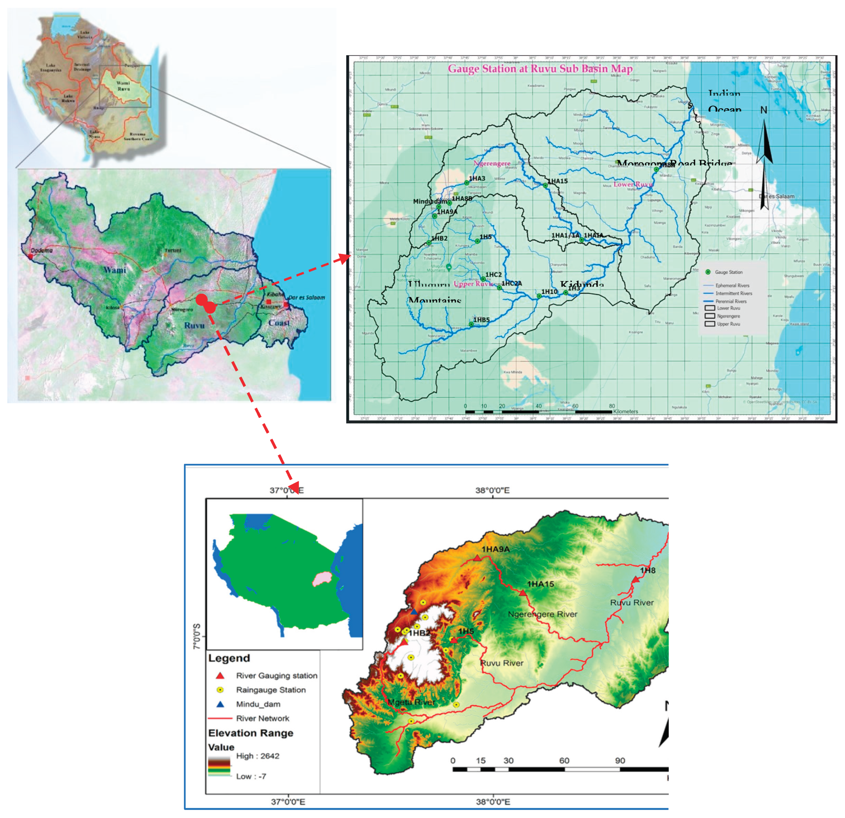
Figure 2.
Data quality analysis – Precipitation.
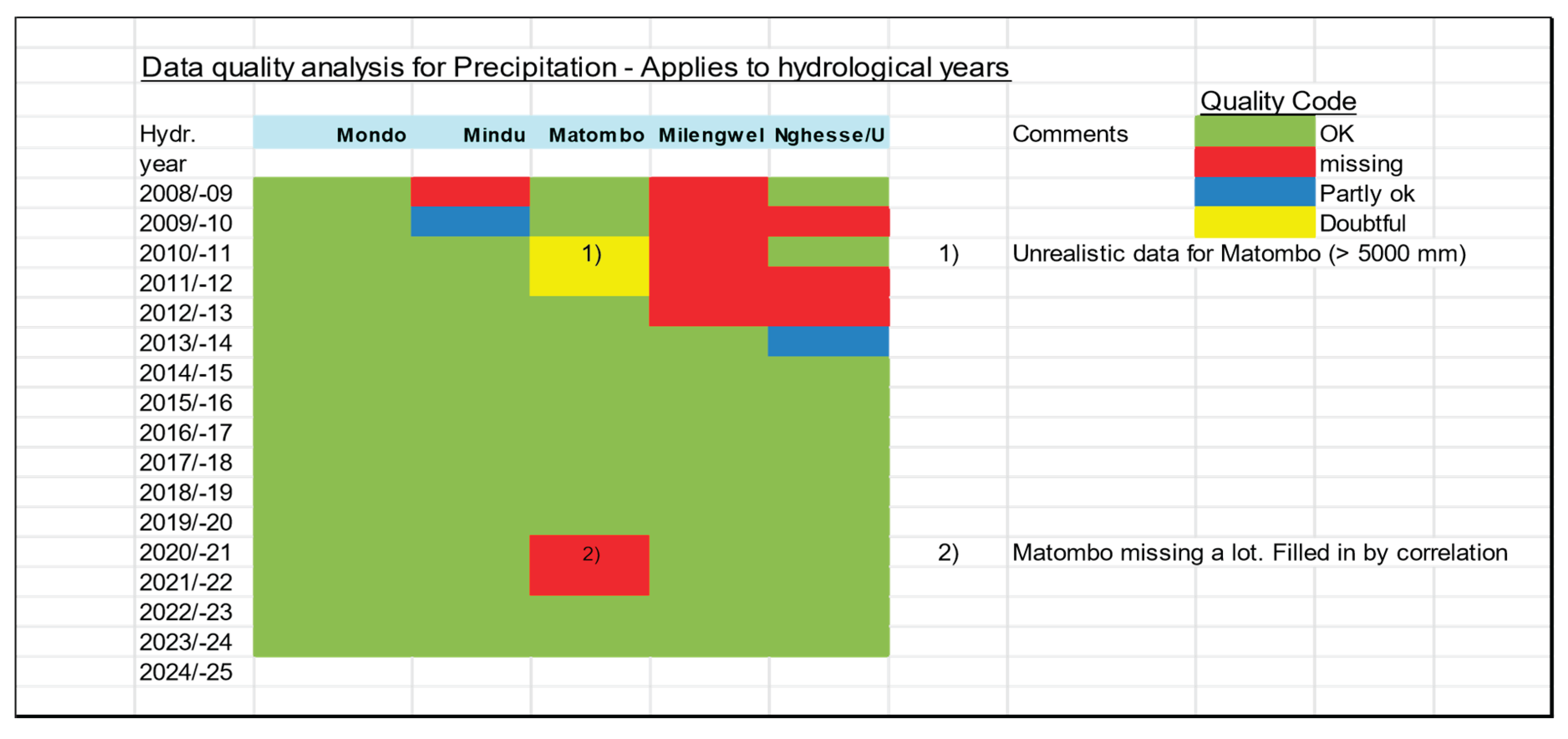
Figure 3.
Data quality analysis – Runoff data.
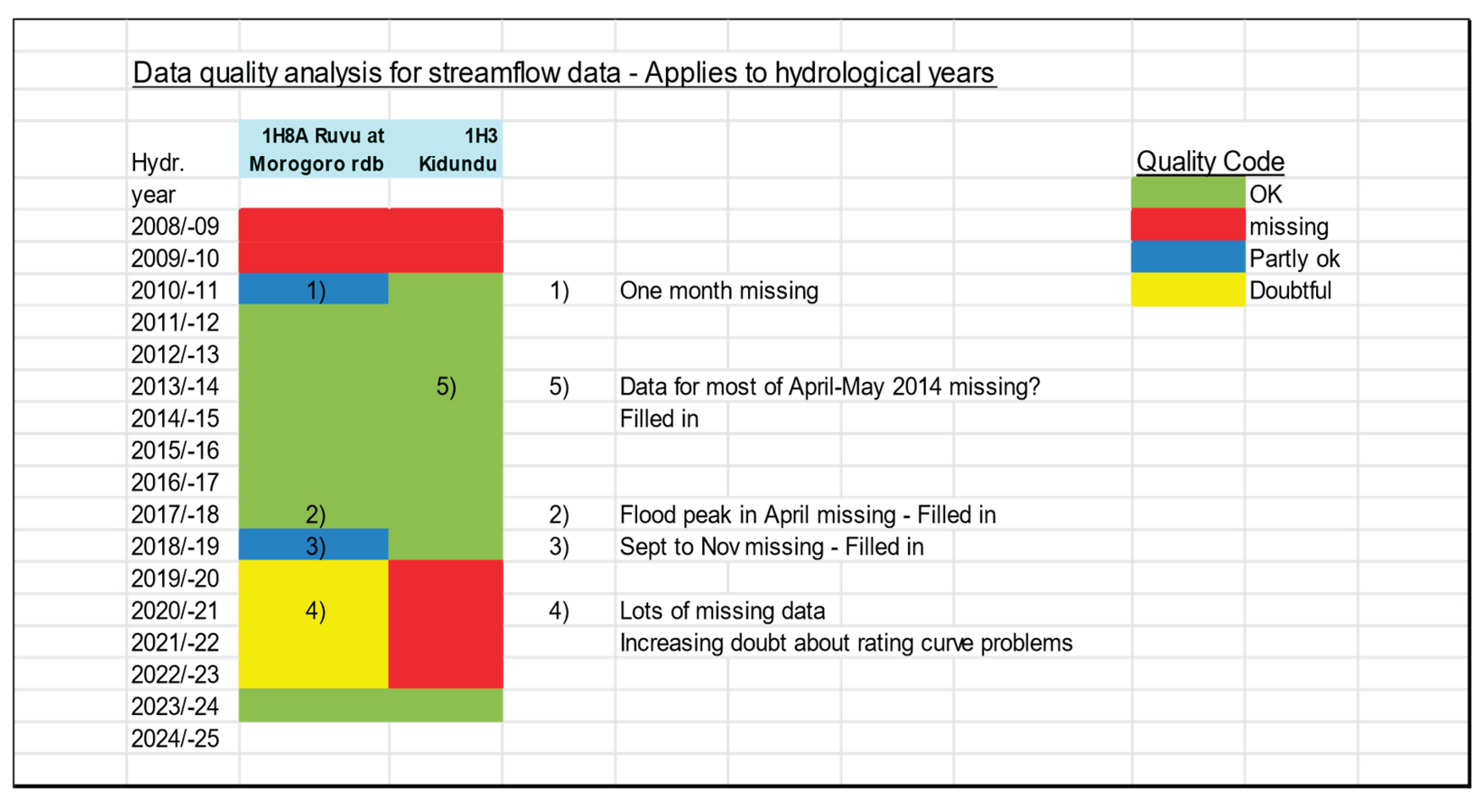
Figure 4.
Location of selected flow gauging stations in the study area.
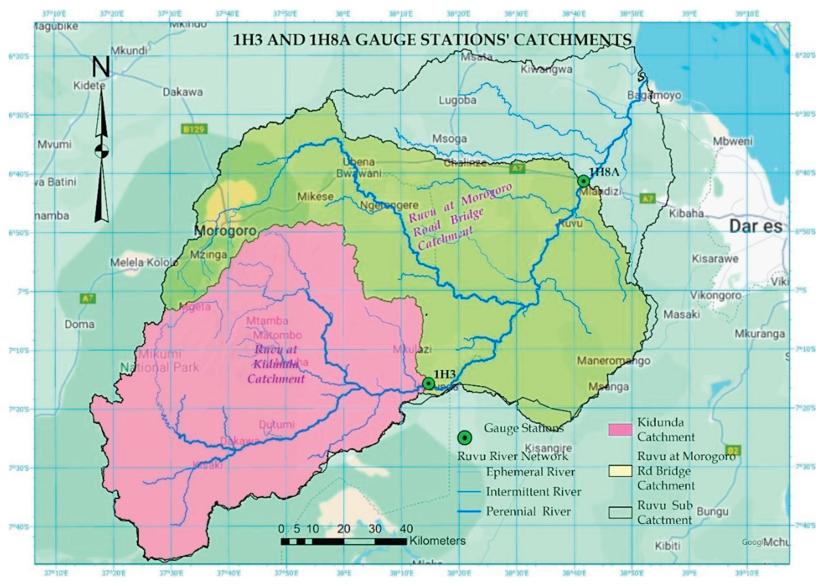
Figure 5.
Climatic data for Ruvu Basin.
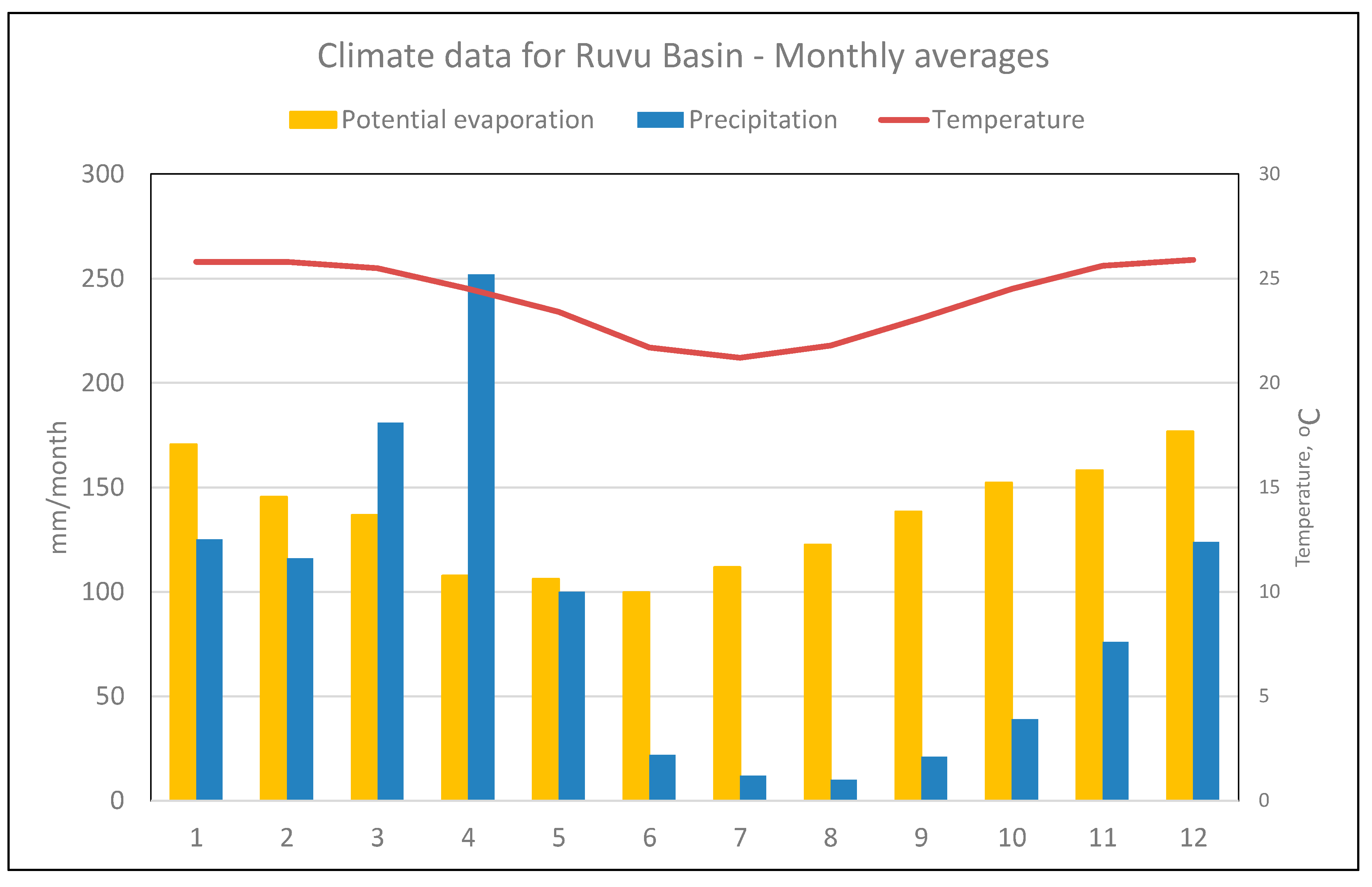
Figure 6.
Ruvu hydrological forecast model system - The 1-stage model system.
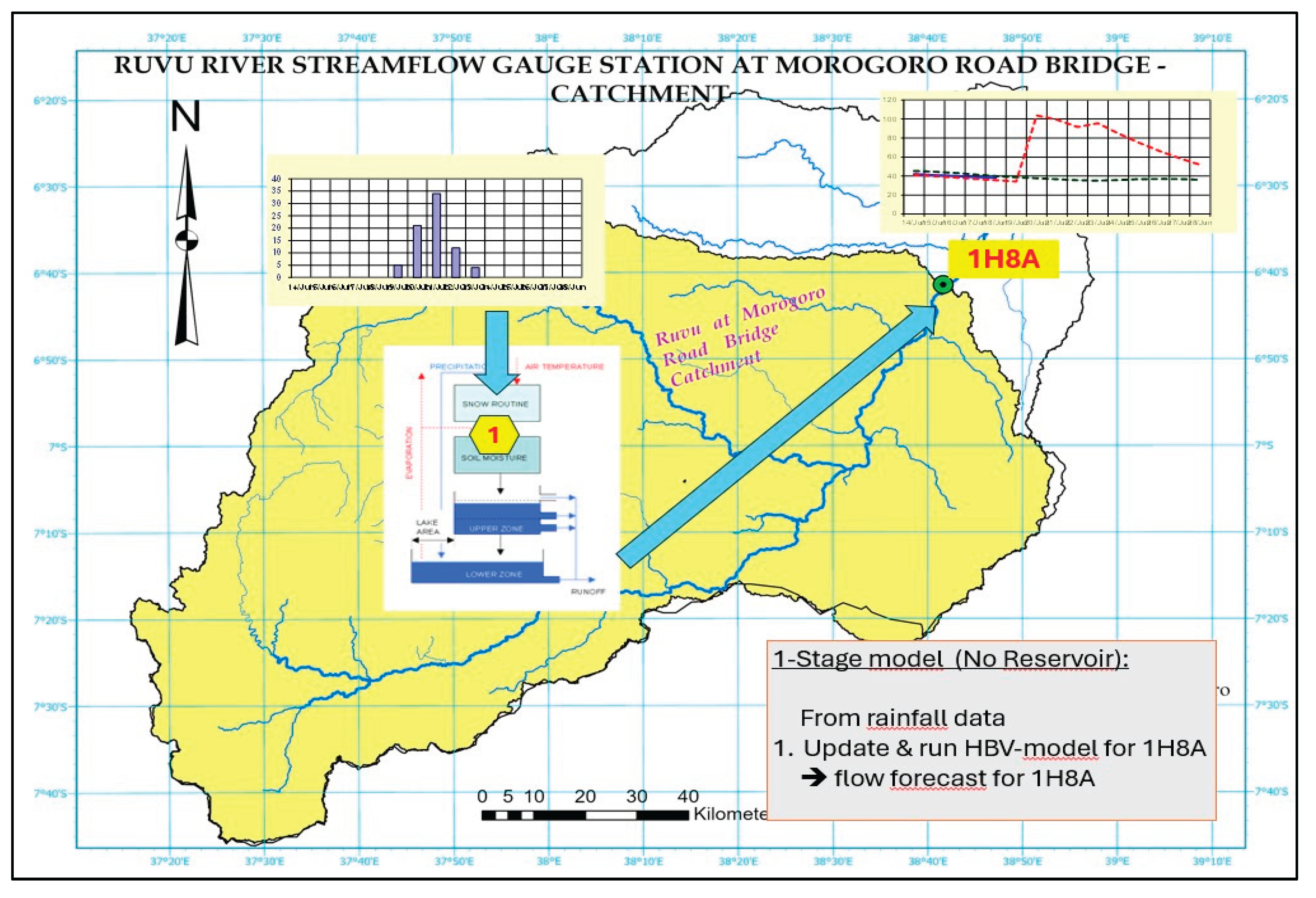
Figure 7.
Ruvu hydrological forecast model system - The 3-stage model system.
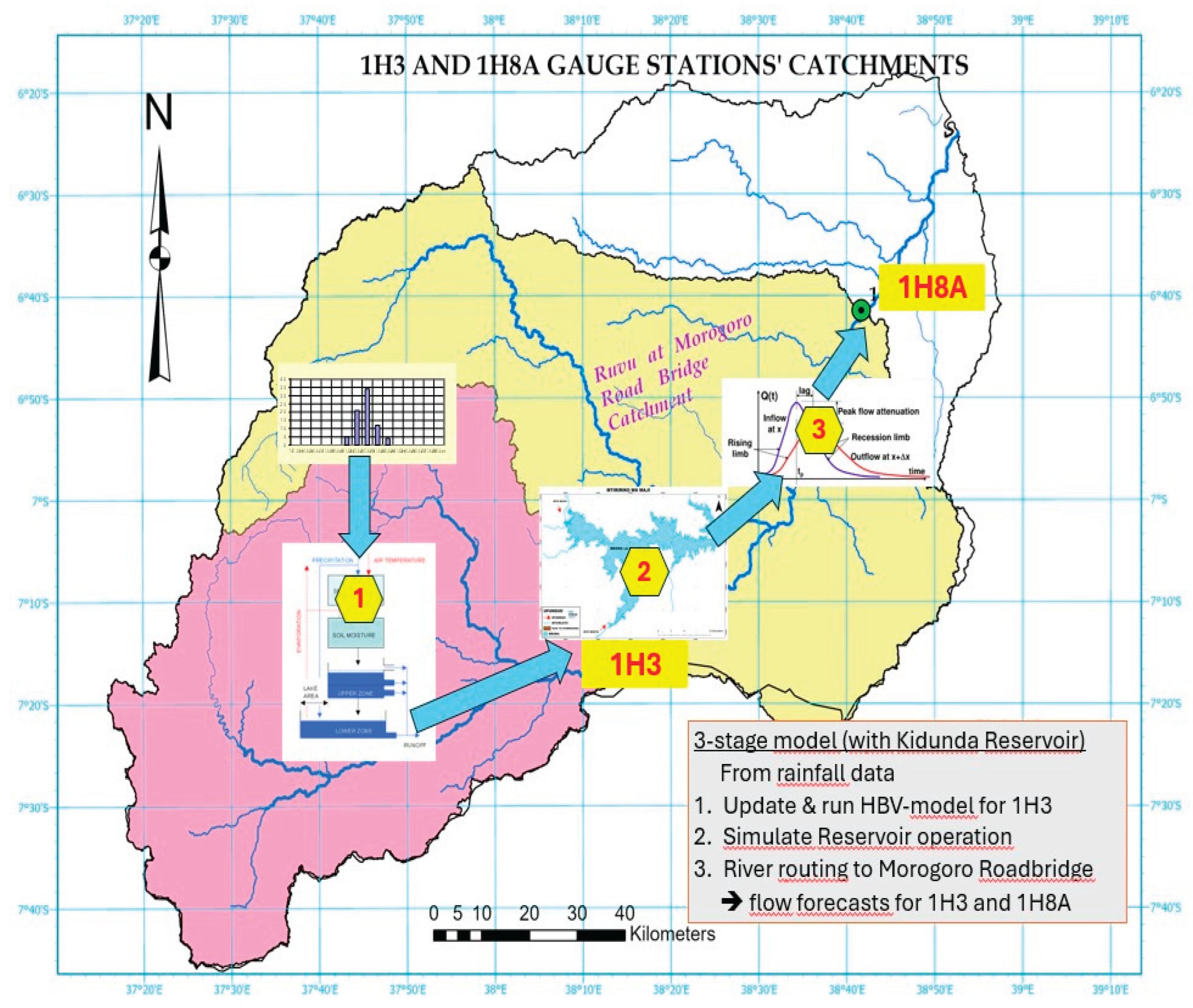
Figure 8.
Ruvu-HBV flow forecasting model – Components and data flow.
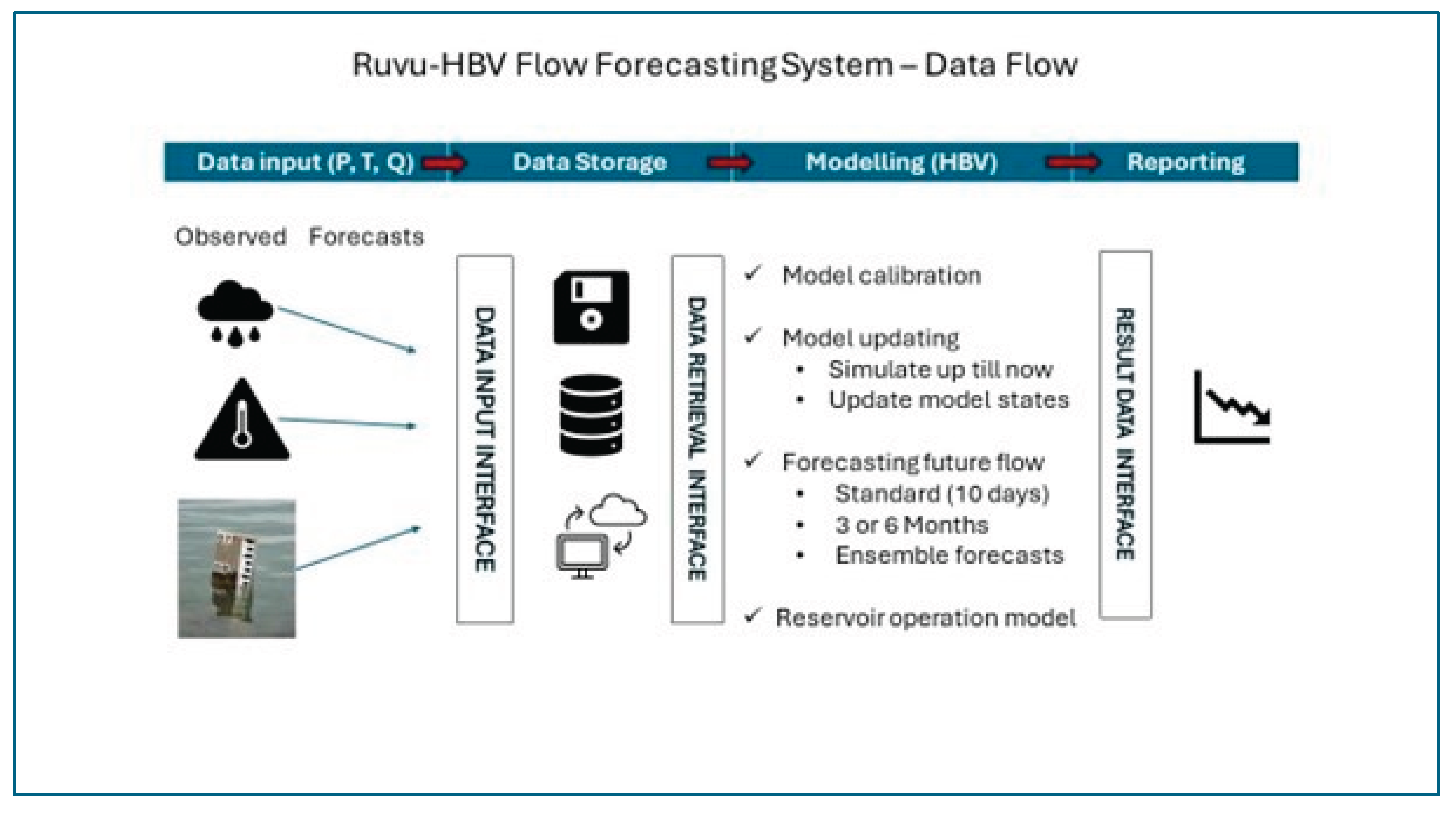
Figure 9.
Proposed GSM Technology for data capture and transmission.
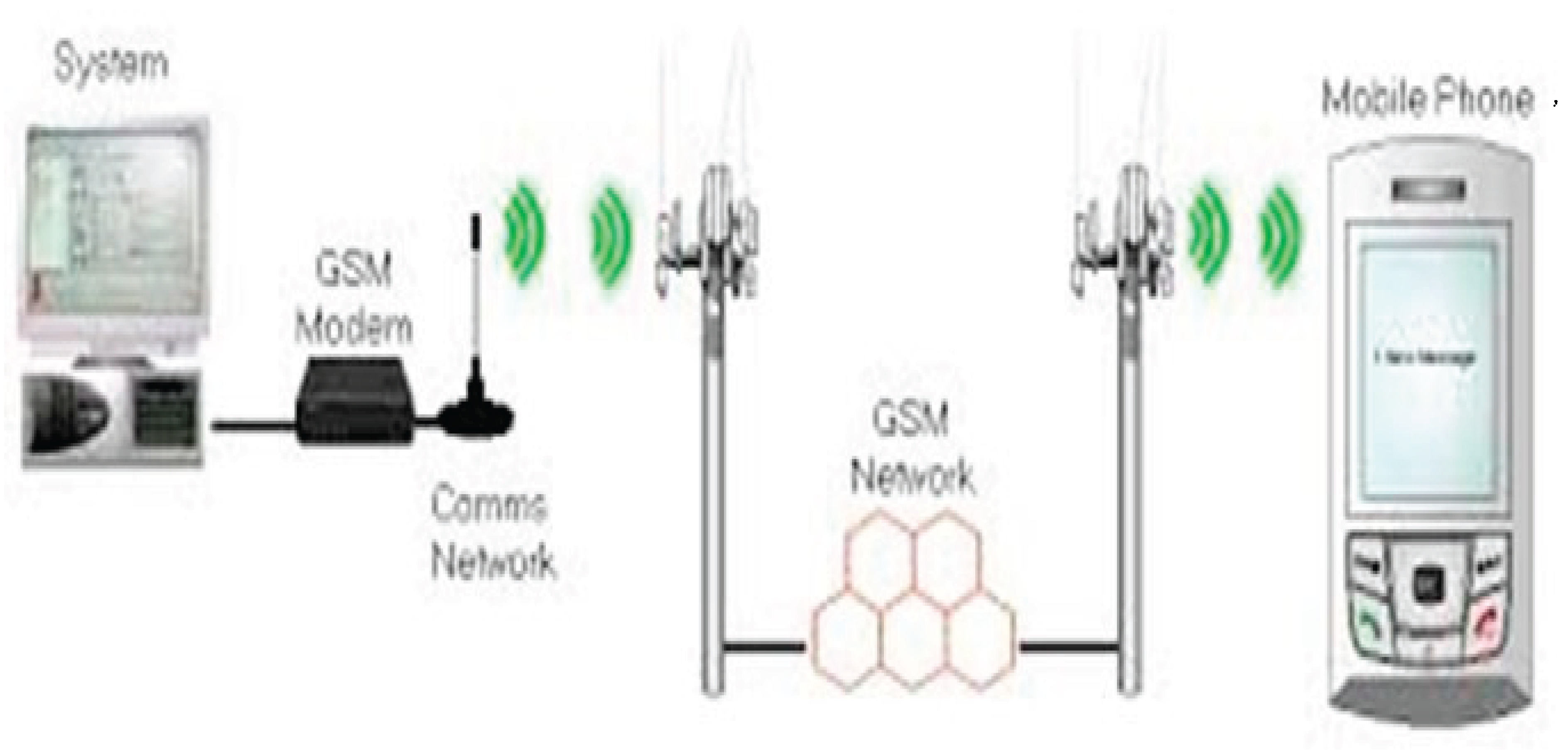
Figure 10.
The HBV-model – Simplified version without snow routine.
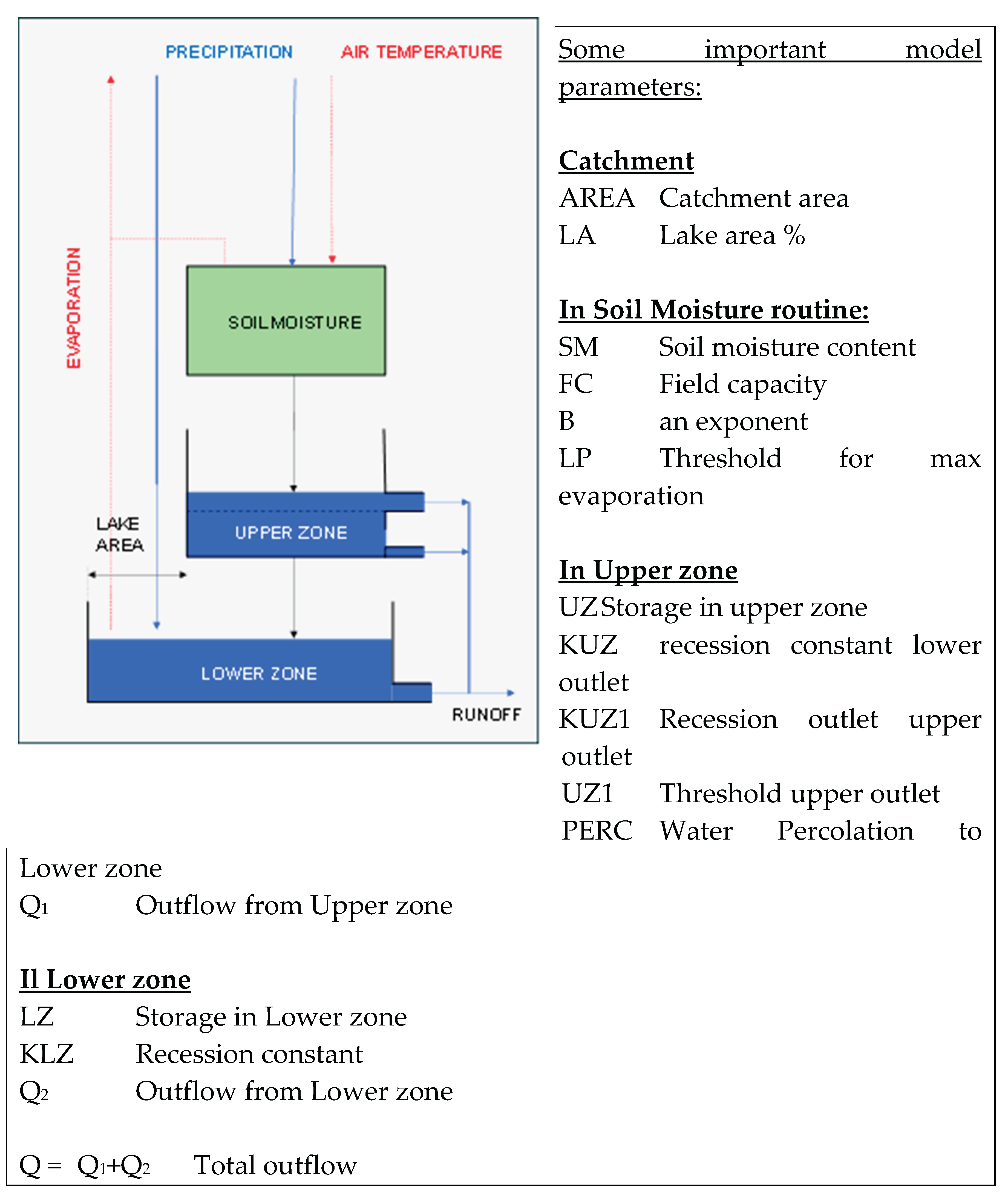
Figure 11.
Operators interface to the Ruvu-HBV streamflow forecasting model.
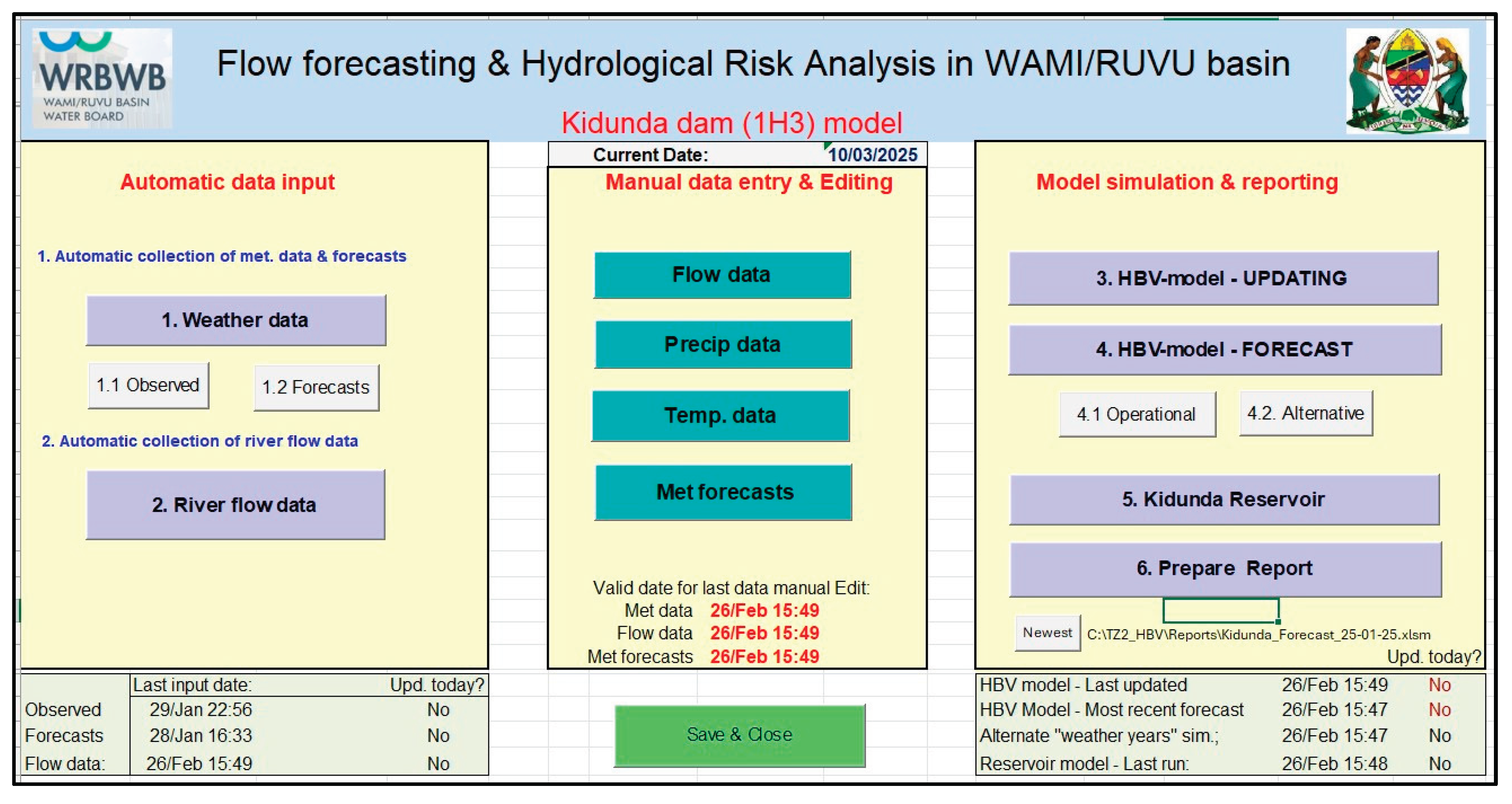
Figure 12.
H8A - Observed and Simulated flow in Calibration period.
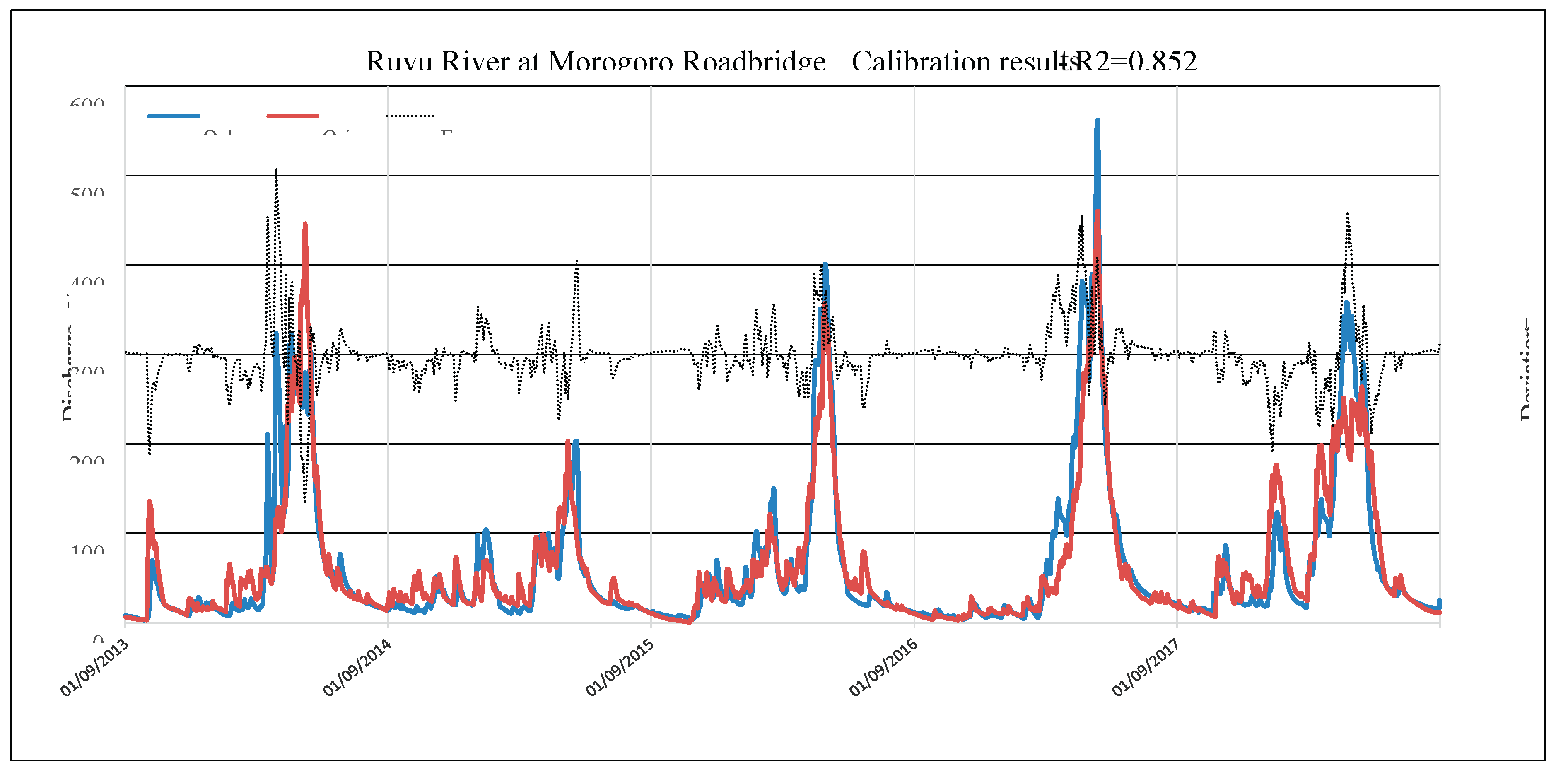
Figure 13.
H8A - Observed and Simulated flow in Verification period.
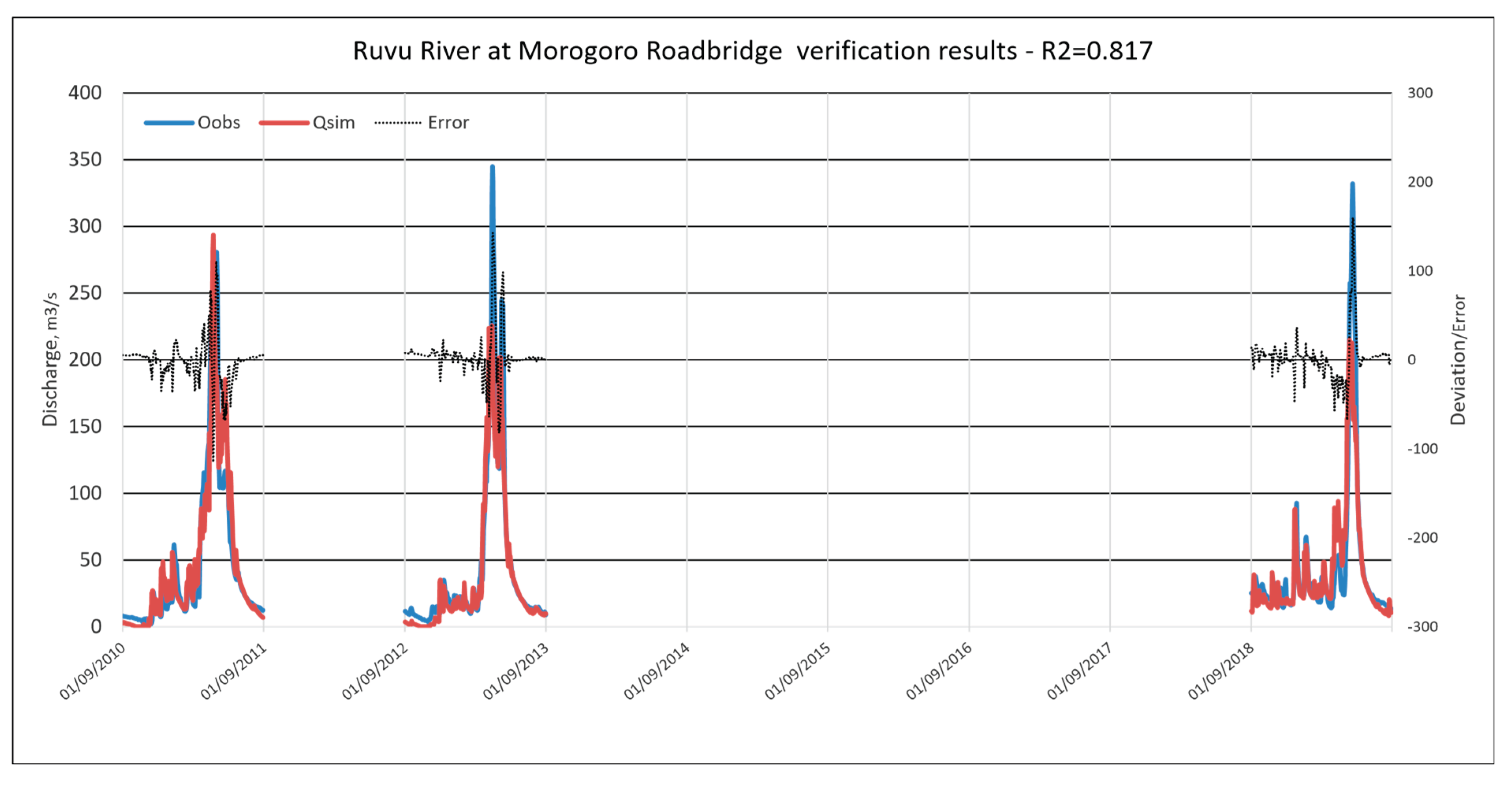
Figure 14.
H8A - Duration curves for Observed and Simulated flow, Calibration period.
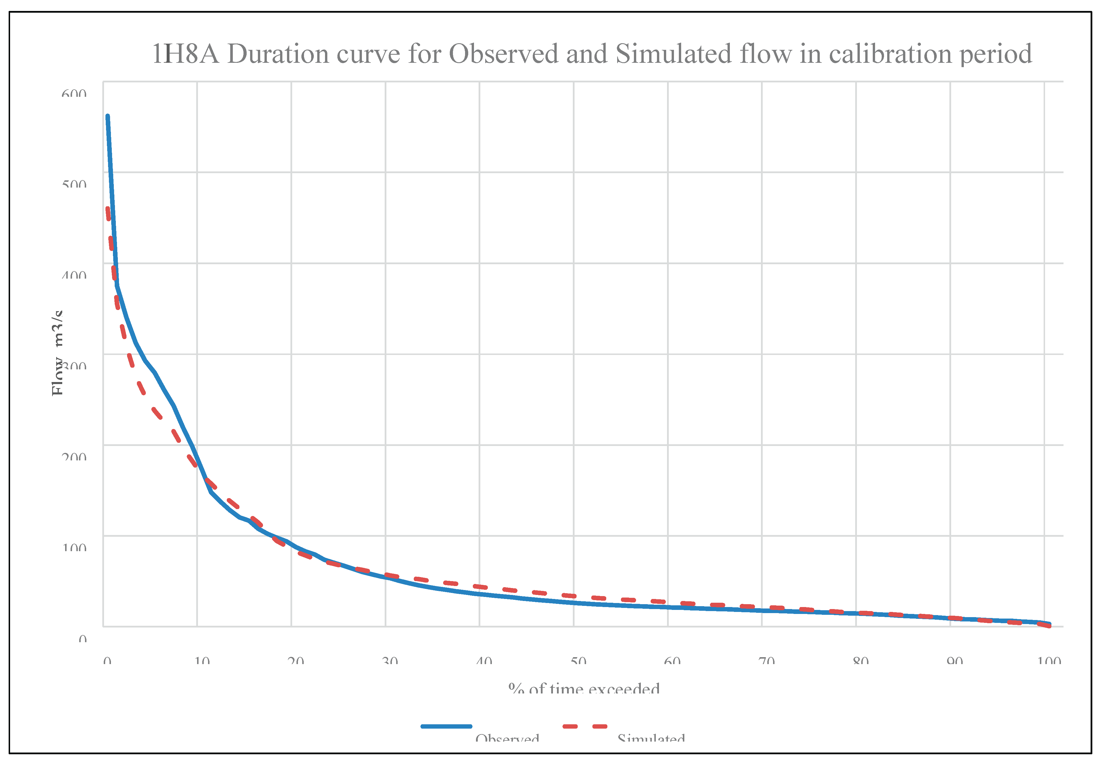
Figure 15.
H8A - Duration curves for Observed and Simulated flow, Verification period.
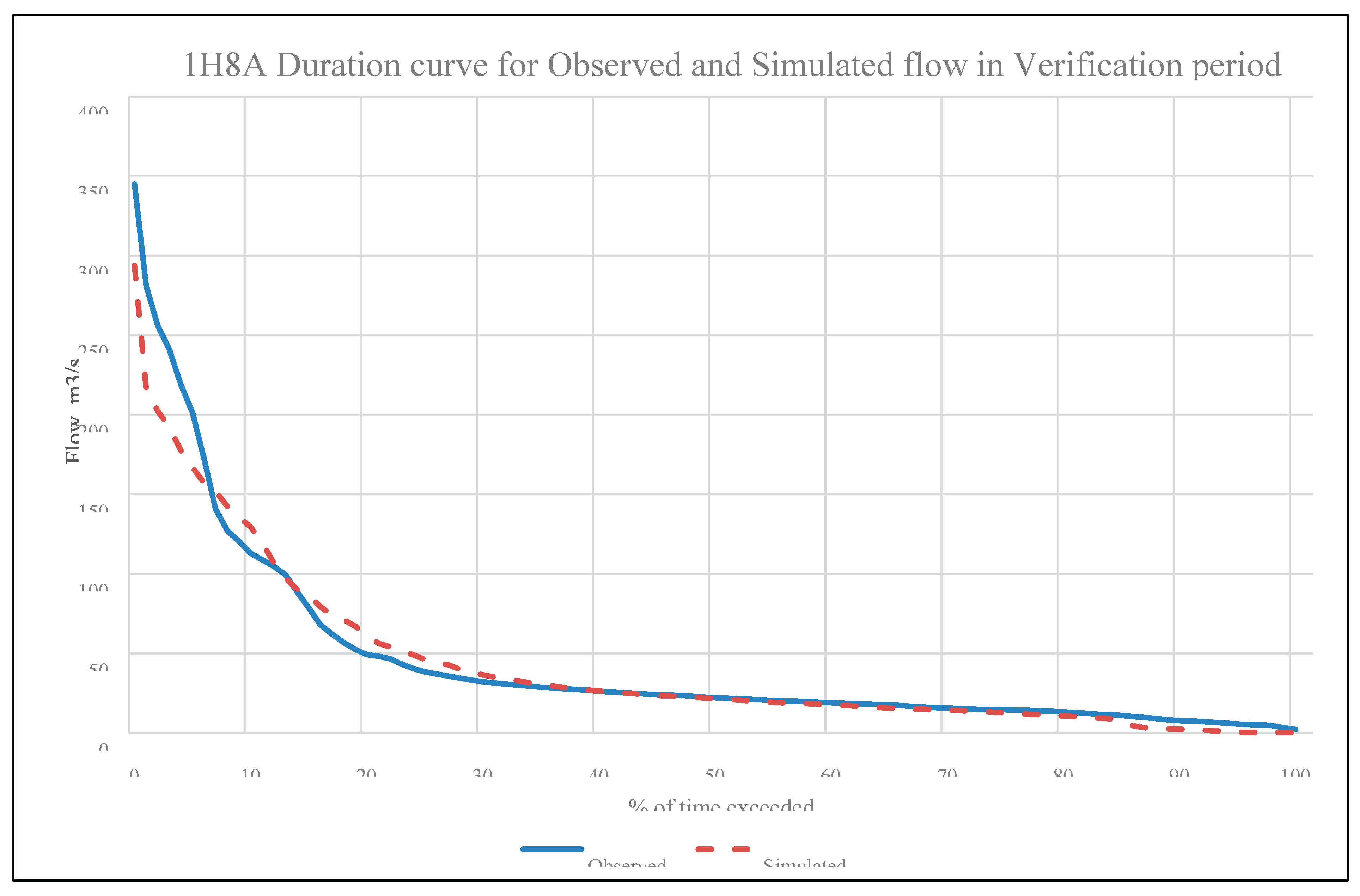
Figure 16.
H3 Kigunda – Observed and Simulated flow in Calibration period.
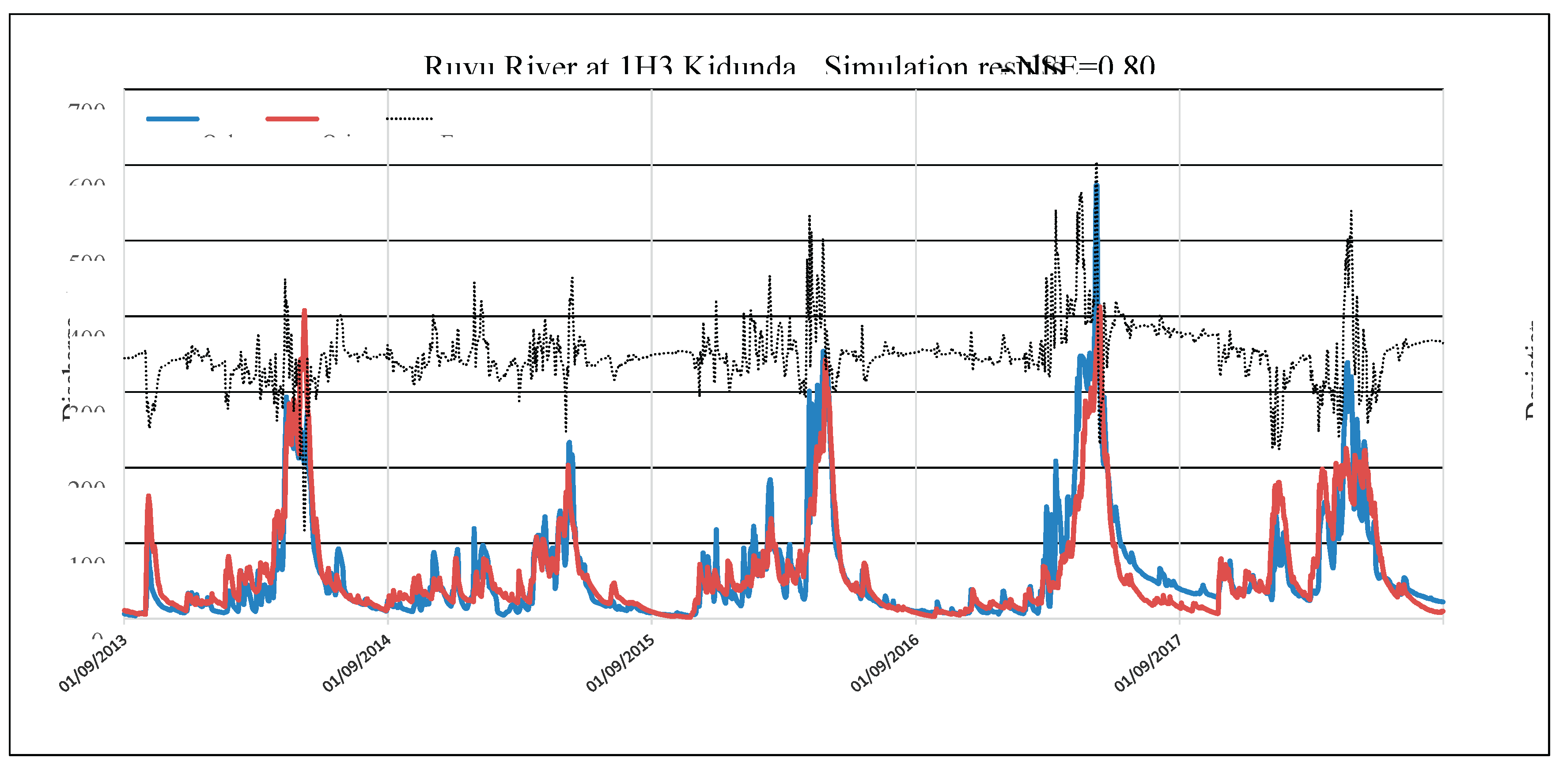
Figure 17.
H3 Kigunda – Observed and Simulated flow in the Verification period.
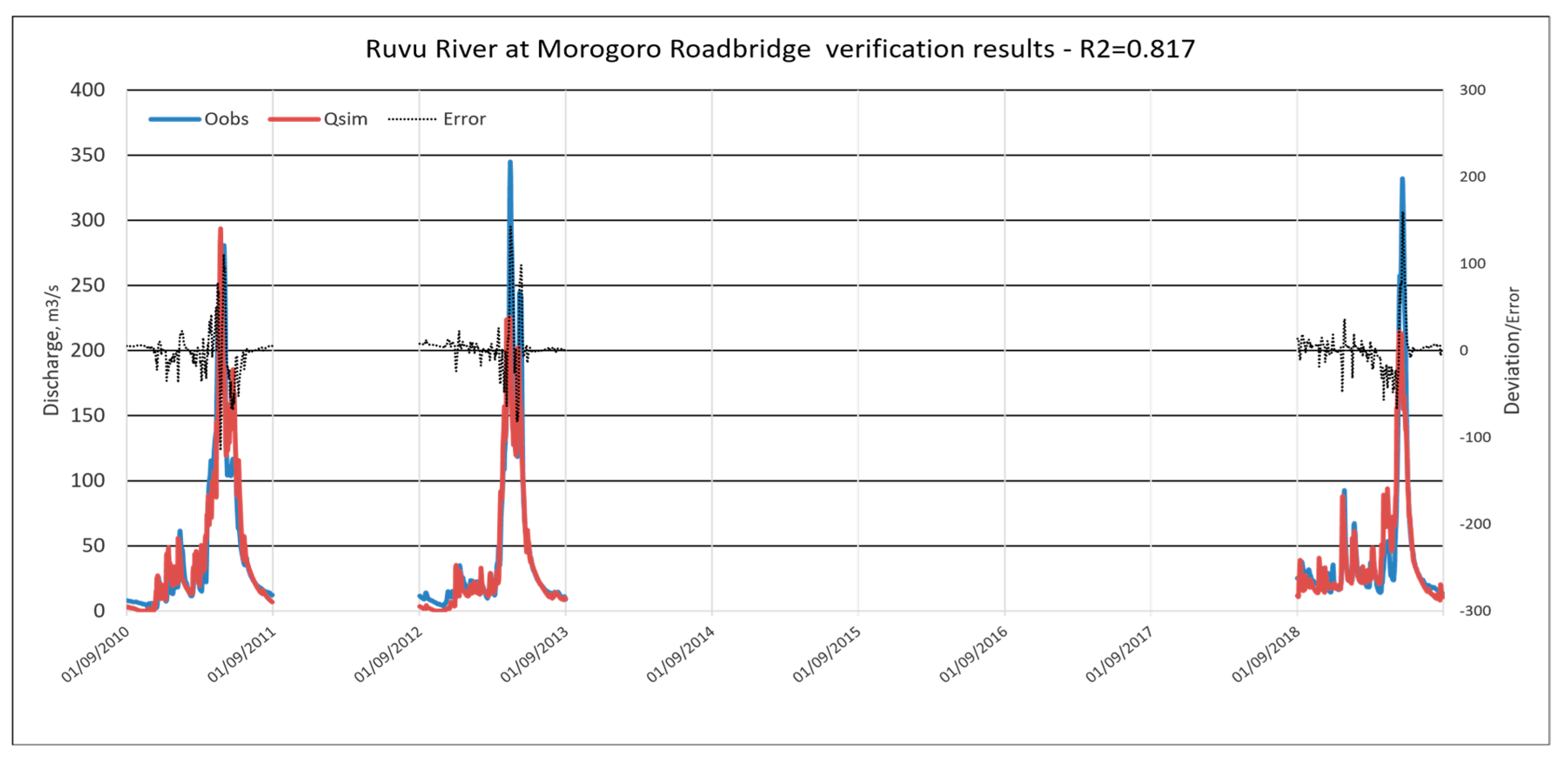
Figure 18.
Day flow forecast issued June 25th for 1H8A Ruvu at Morogoro Roadbridge.
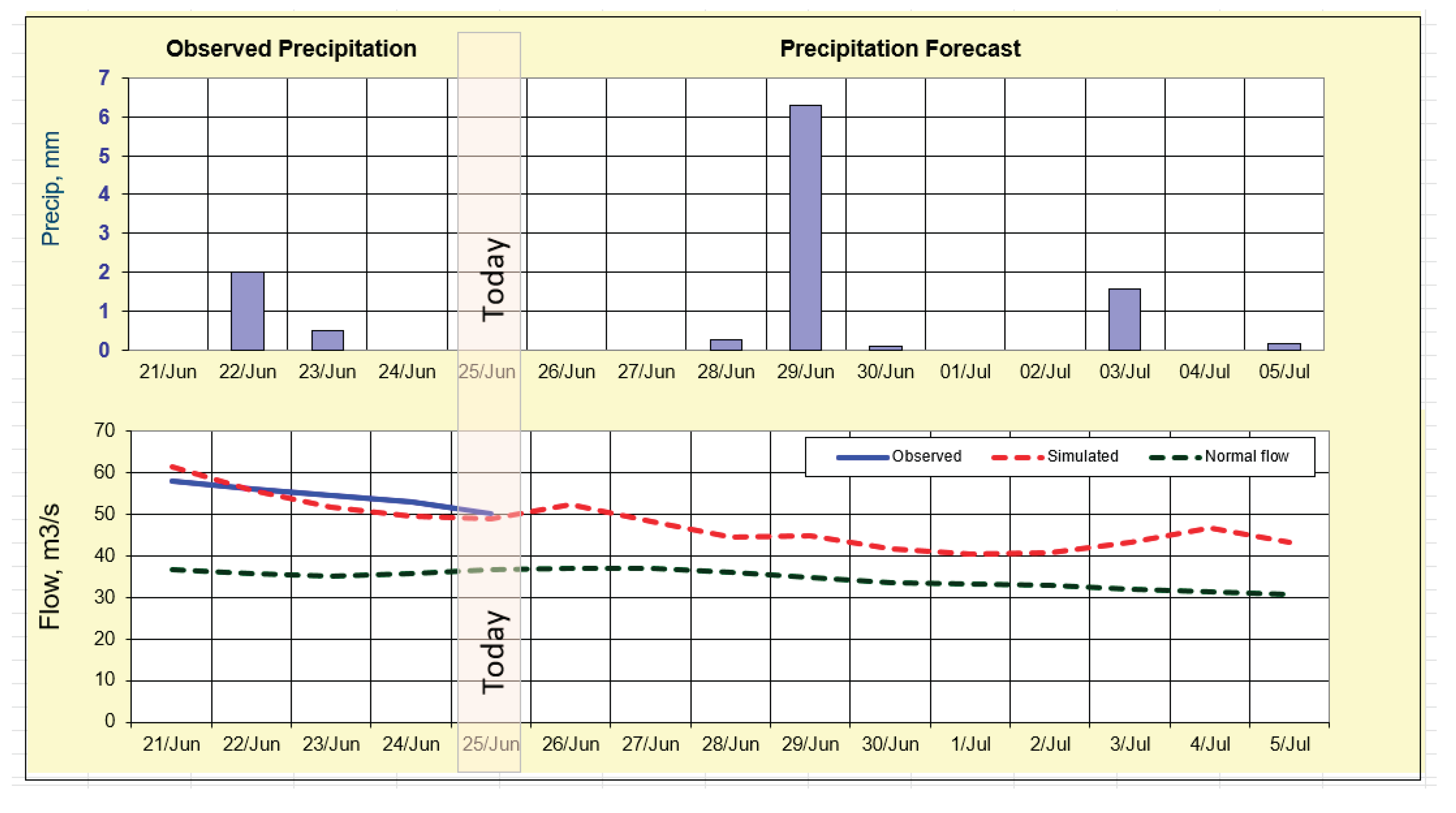
Figure 19.
Alternative forecasts for 1H3 Kidunda - Sensitivity to precipitation volume.
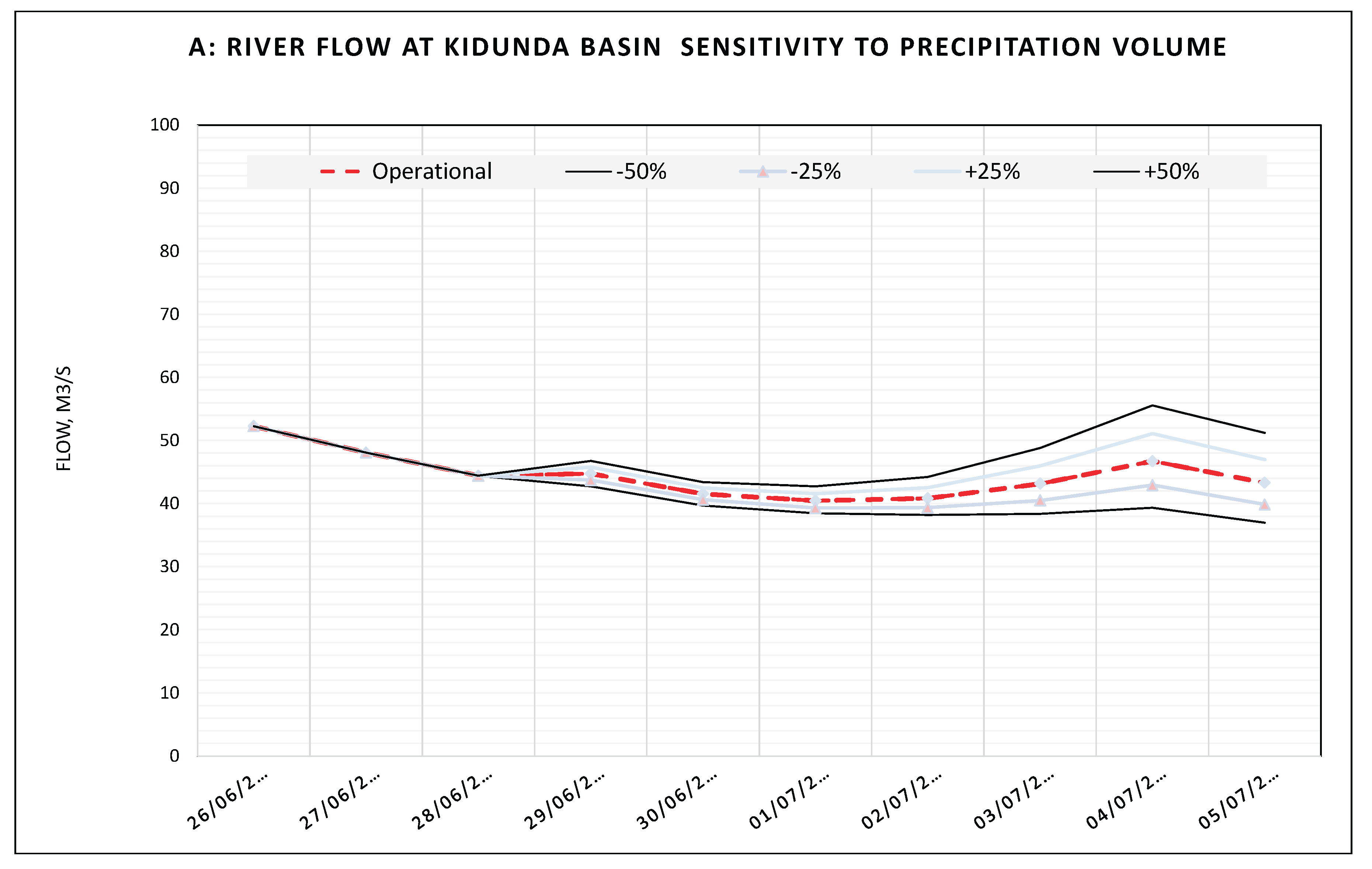
Figure 20.
Alternative "forecasts" for 1H3 Kidunda for 5 different "weather years".
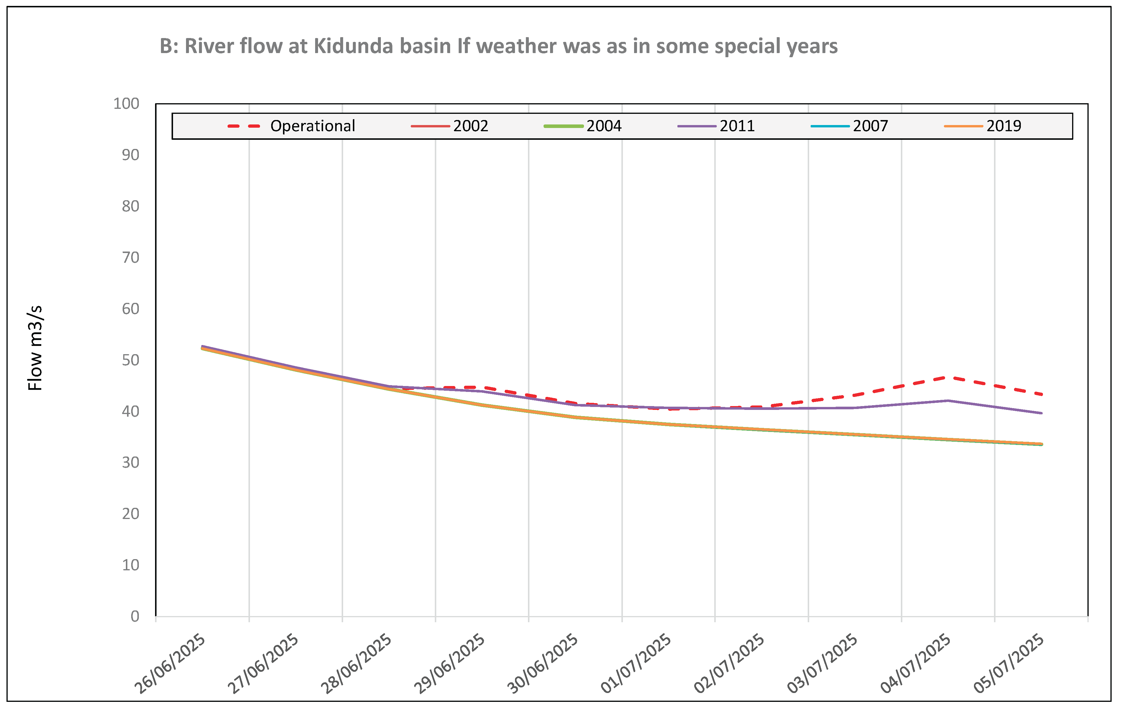
Figure 21.
Ruvu at Morogoro Roadbridge - Seasonal flow forecast for September to November 2025.
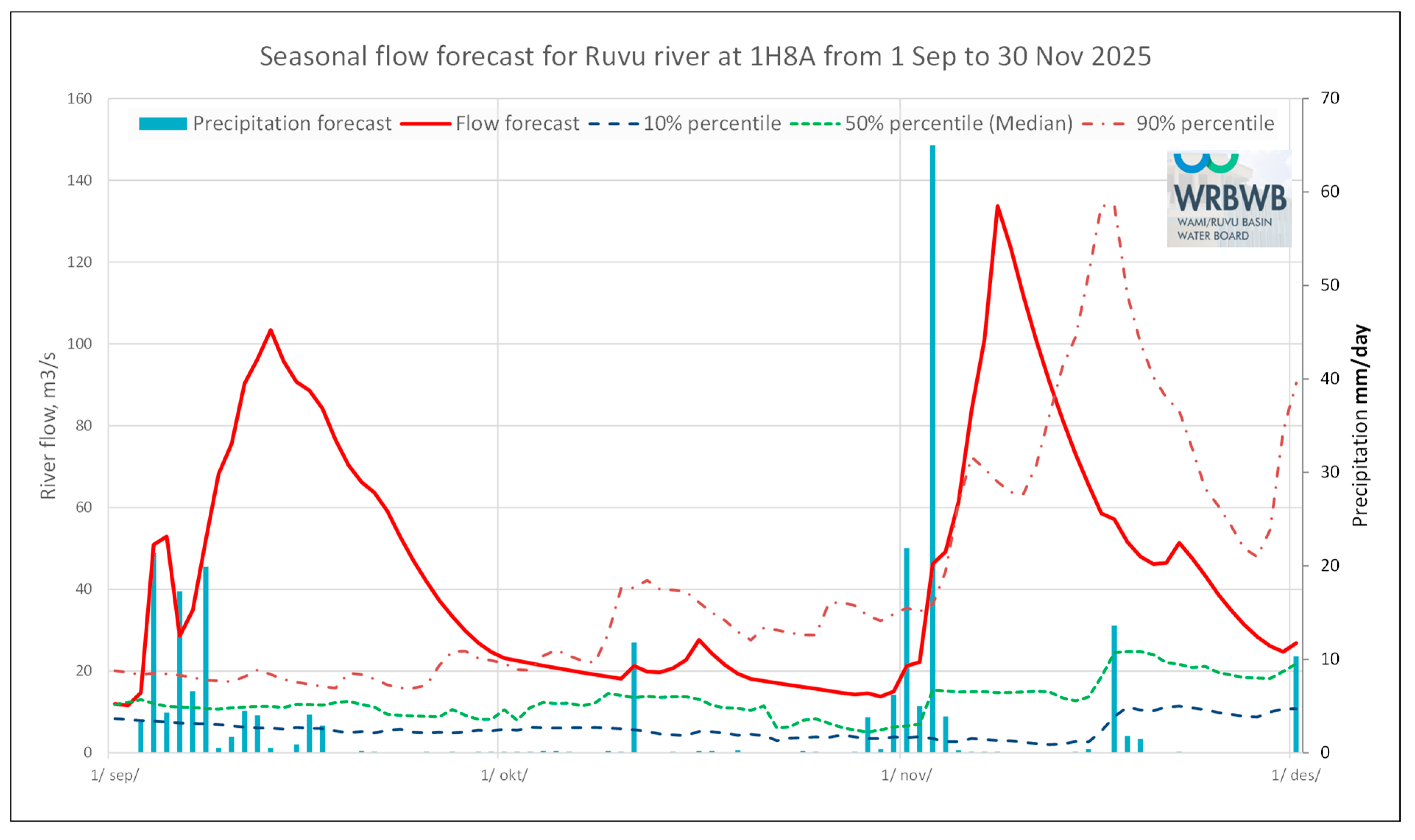
Figure 22.
Ruvu at Morogoro Roadbridge - Volume of flow in the seasonal forecast 1st Sep to 30th Nov.compared to previous years 2009-2024.
Figure 22.
Ruvu at Morogoro Roadbridge - Volume of flow in the seasonal forecast 1st Sep to 30th Nov.compared to previous years 2009-2024.
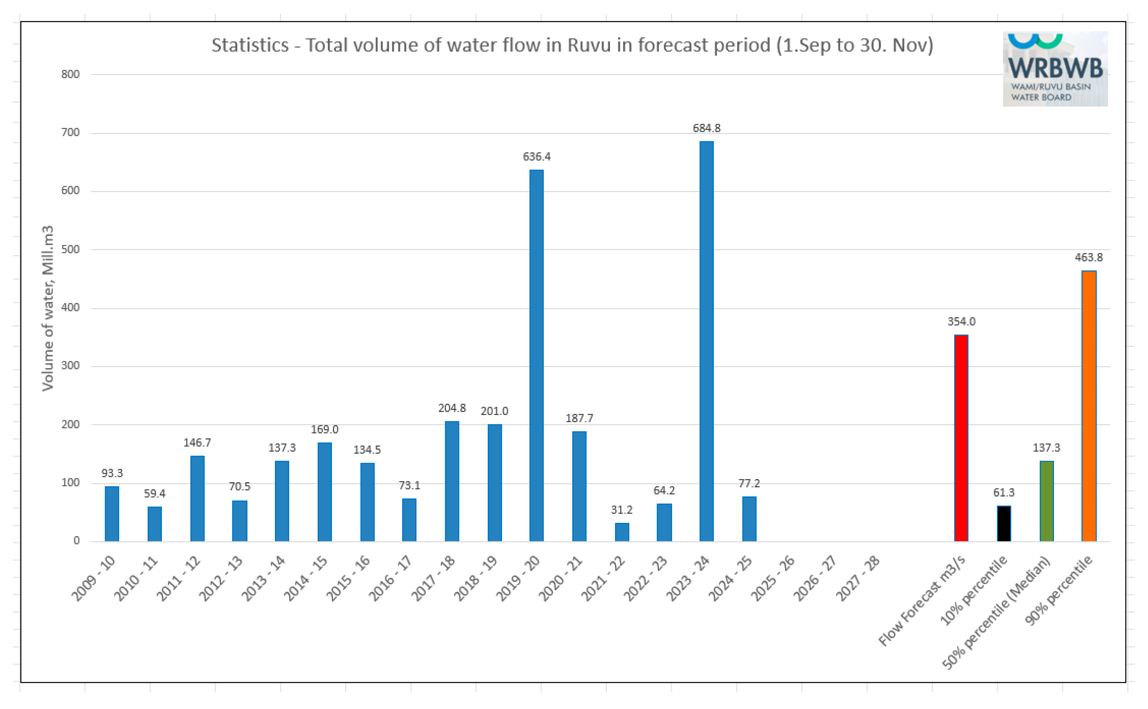
Figure 23.
Streamflow forecasts in Dry season for station 1H8A Ruvu at Morogoro Roadbridge. Forecast based on 10-day precipitation forecasts from (TMA) and Yr.
Figure 23.
Streamflow forecasts in Dry season for station 1H8A Ruvu at Morogoro Roadbridge. Forecast based on 10-day precipitation forecasts from (TMA) and Yr.
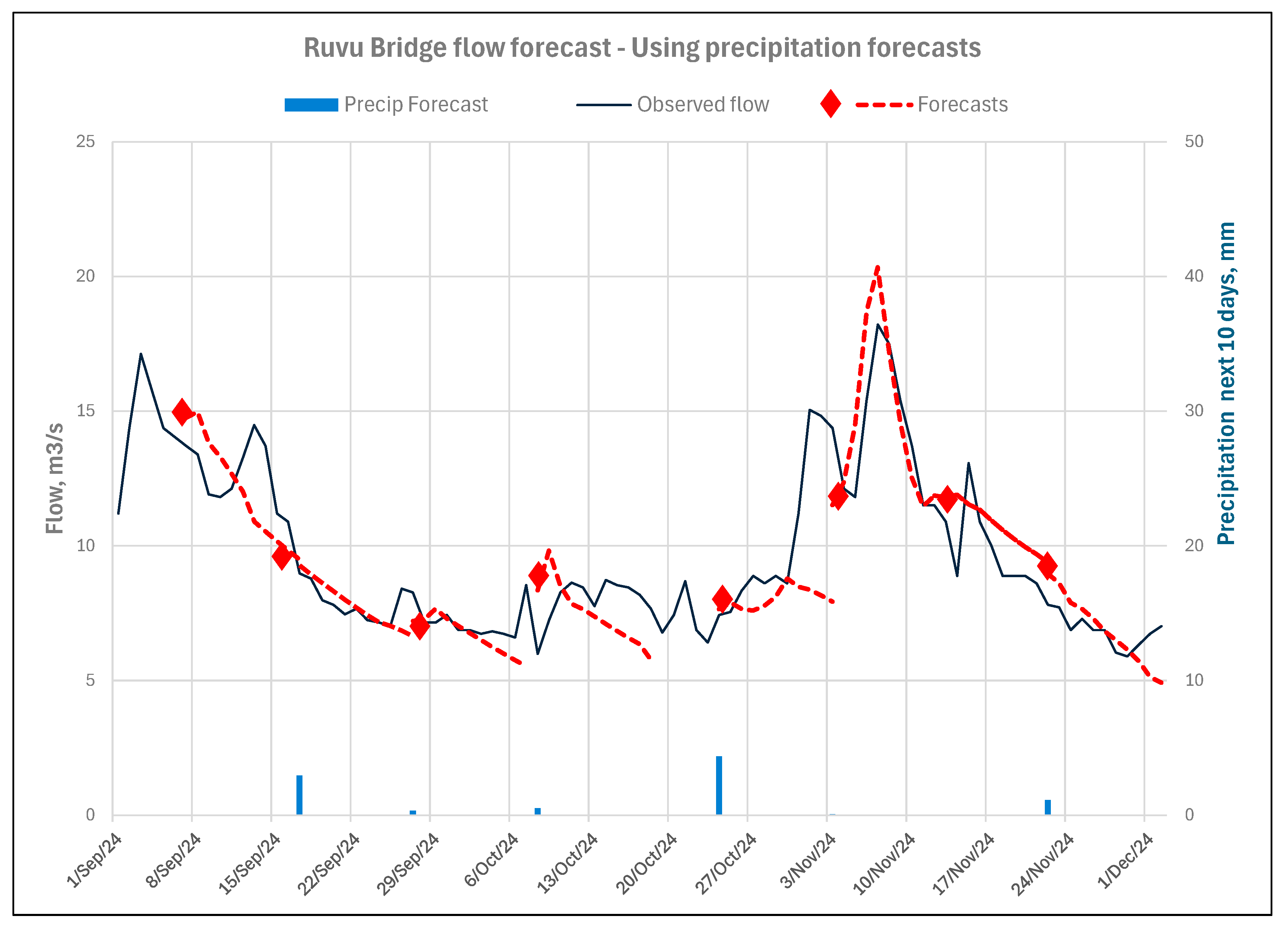
Figure 24.
Streamflow forecasts in Dry season for station 1H8A Ruvu at Morogoro Roadbridge assuming a perfect forecast of precipitation (Observed precipitation).
Figure 24.
Streamflow forecasts in Dry season for station 1H8A Ruvu at Morogoro Roadbridge assuming a perfect forecast of precipitation (Observed precipitation).
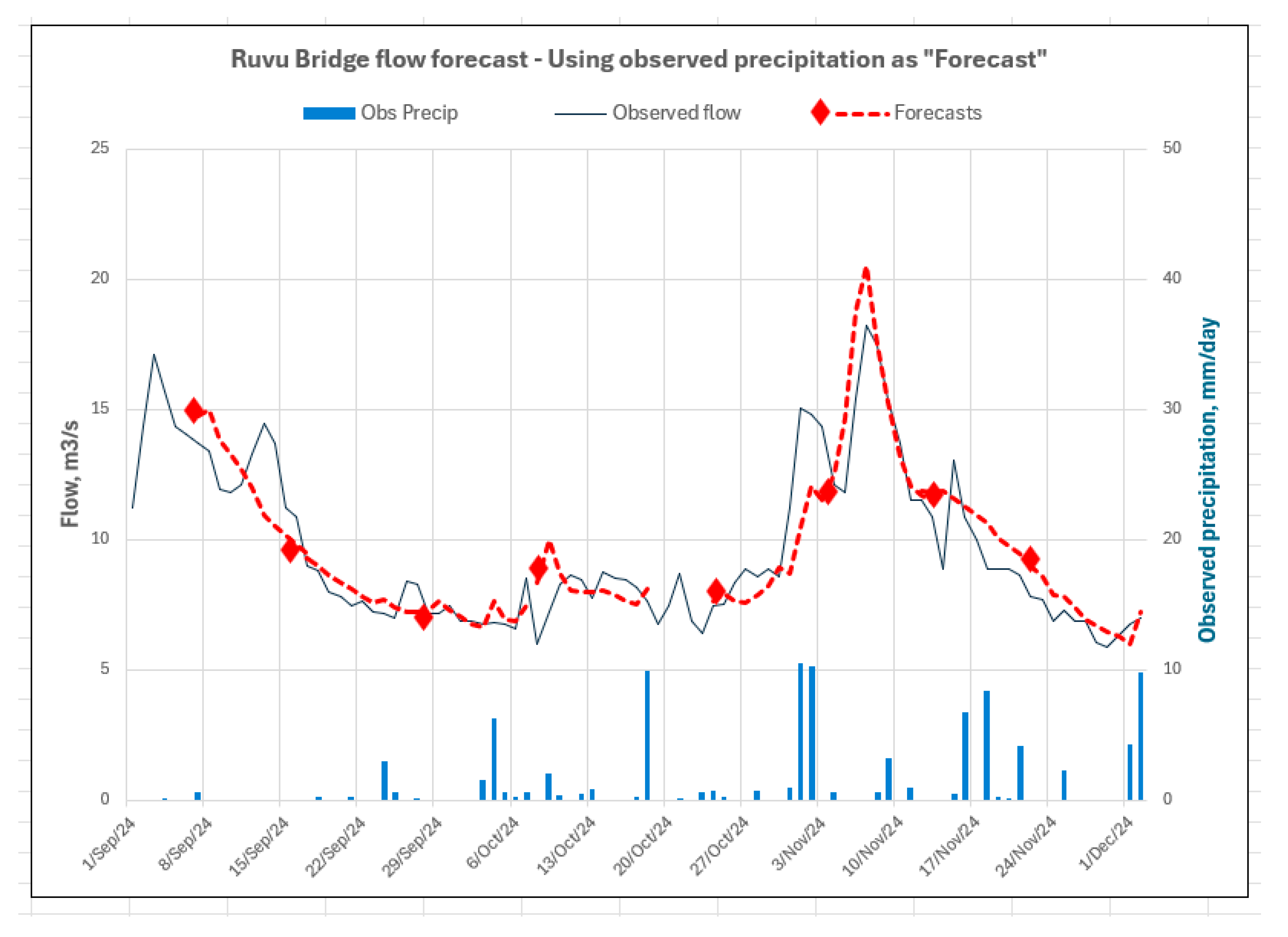
Figure 25.
Streamflow forecasts for 1H8A Morogoro Roadbridge in the Short-Rains season. Forecasts are based on 10-day precipitation forecasts from TMA/Yr.
Figure 25.
Streamflow forecasts for 1H8A Morogoro Roadbridge in the Short-Rains season. Forecasts are based on 10-day precipitation forecasts from TMA/Yr.

Figure 26.
Streamflow forecasts in the Short-rain season for station 1H8A Ruvu at Morogoro Roadbridge assuming a perfect forecast of precipitation (Observed precipitation).
Figure 26.
Streamflow forecasts in the Short-rain season for station 1H8A Ruvu at Morogoro Roadbridge assuming a perfect forecast of precipitation (Observed precipitation).
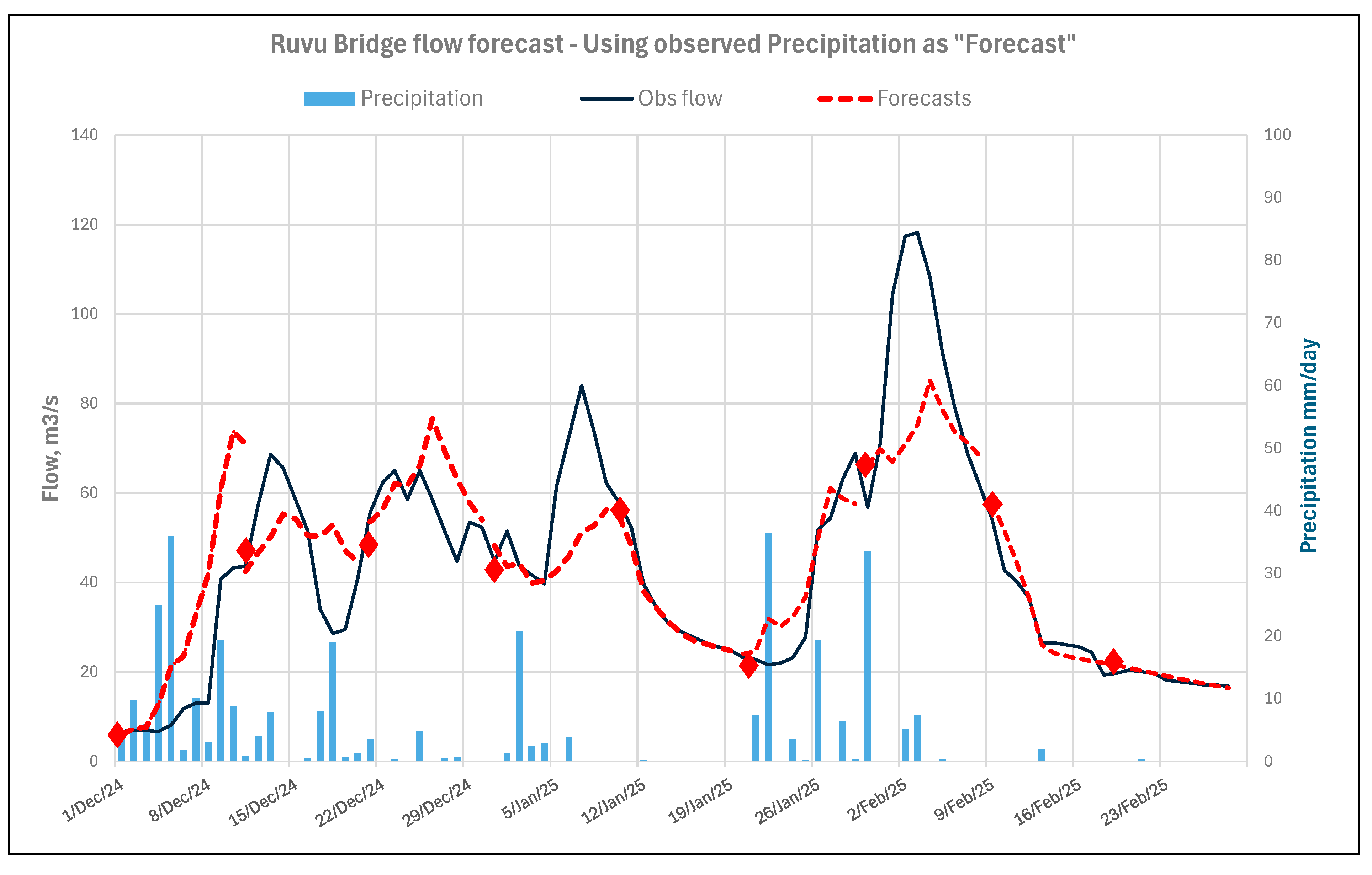
Figure 27.
Streamflow forecasts for 1H8A Ruvu in the Long-Rains season at Morogoro Roadbridge. Forecasts based on 10-day precipitation forecasts from TMA/Yr.
Figure 27.
Streamflow forecasts for 1H8A Ruvu in the Long-Rains season at Morogoro Roadbridge. Forecasts based on 10-day precipitation forecasts from TMA/Yr.
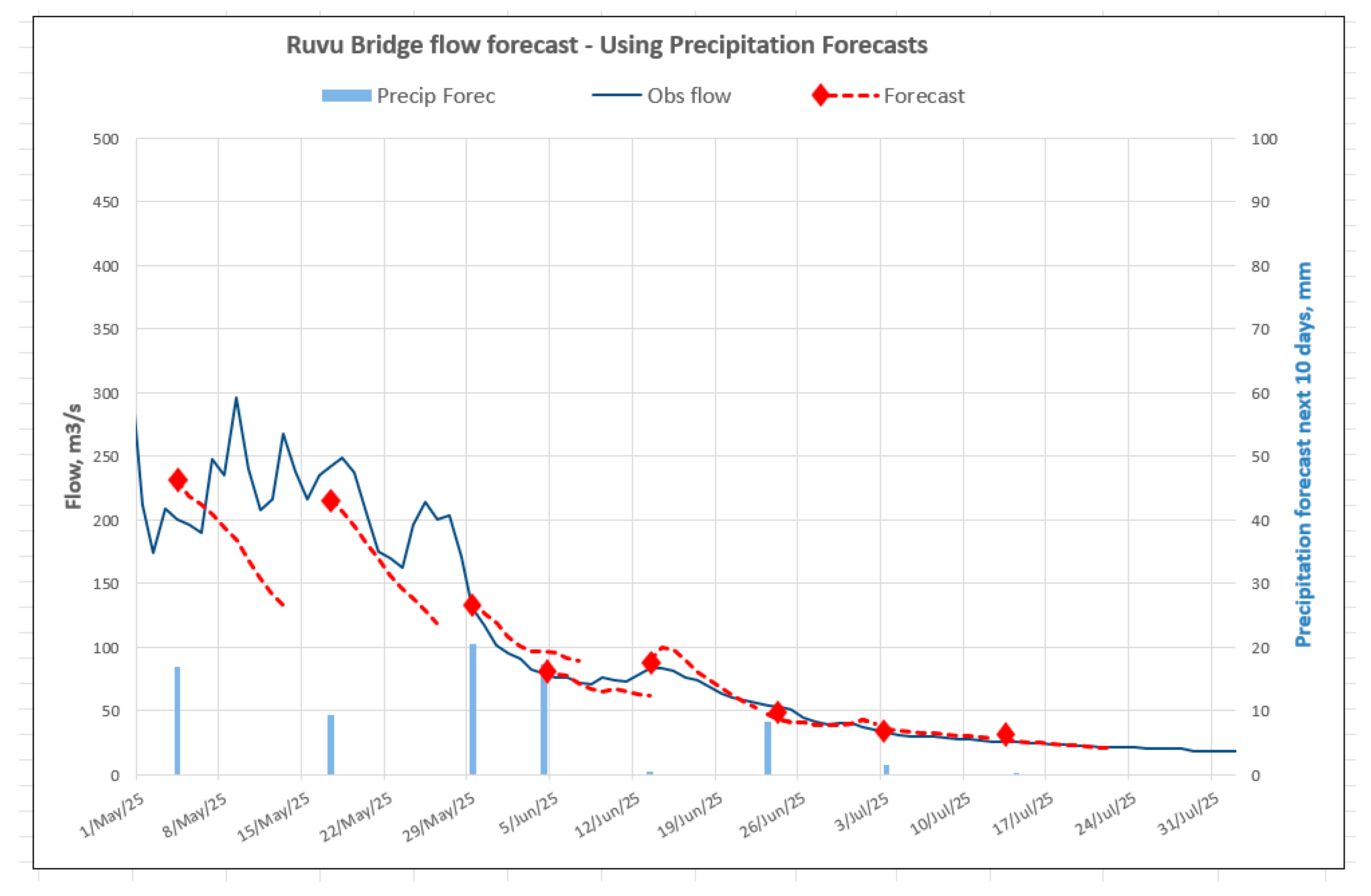
Figure 28.
Streamflow forecasts in the Long-Rain season for station 1H8A Ruvu at Morogoro Roadbridge assuming a perfect forecast of precipitation (Observed precipitation).
Figure 28.
Streamflow forecasts in the Long-Rain season for station 1H8A Ruvu at Morogoro Roadbridge assuming a perfect forecast of precipitation (Observed precipitation).

Figure 29.
Daily flow forecast precision - Dry season.
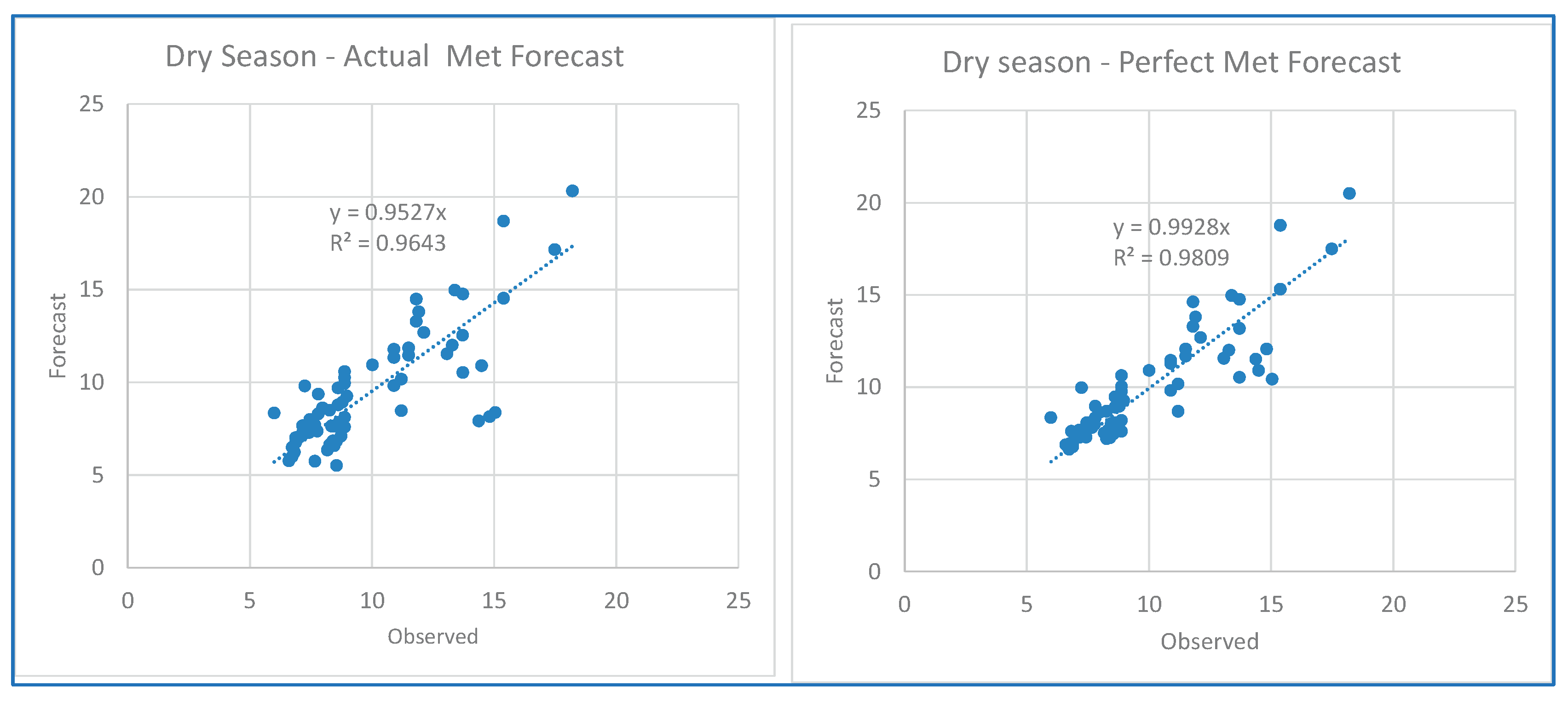
Figure 30.
Daily flow forecast precision – Short Rains season.
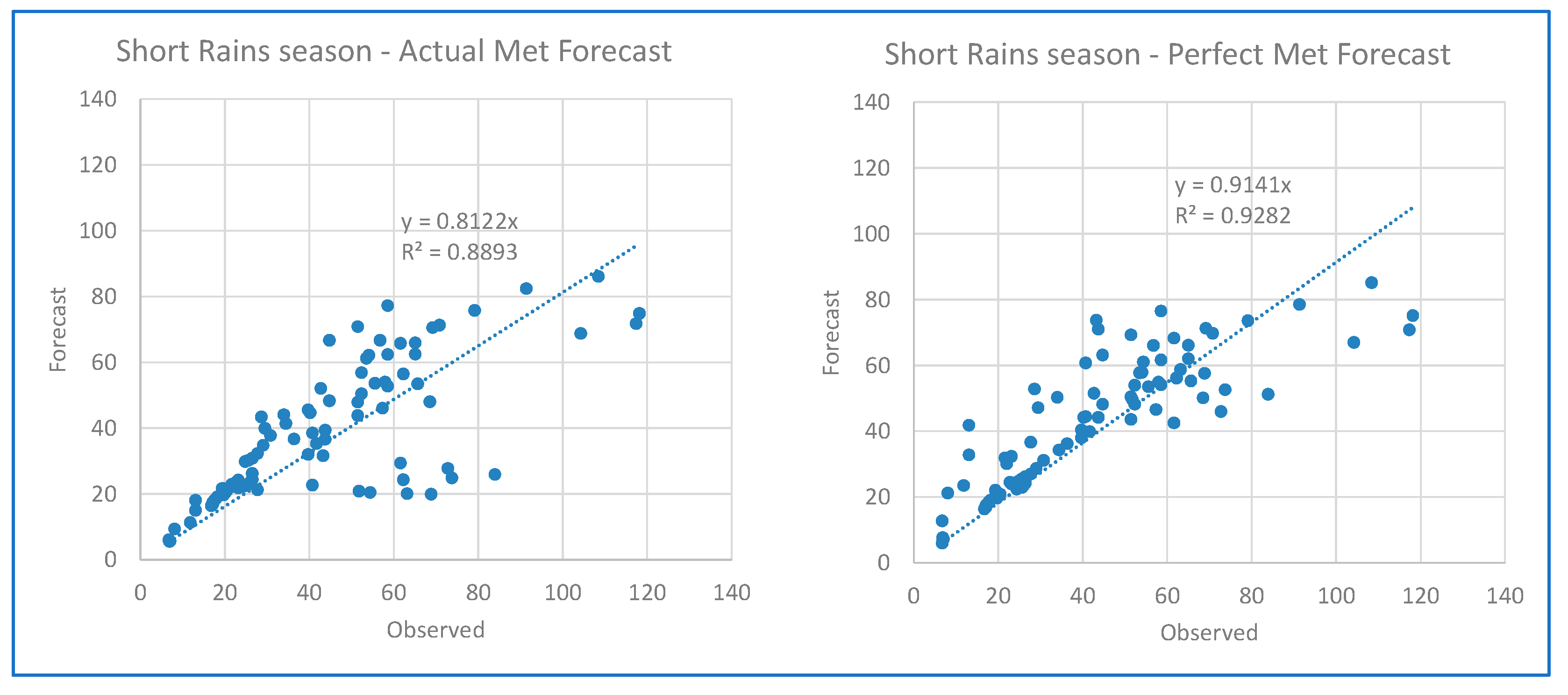
Figure 31.
Daily flow forecast precision – Long Rains season.
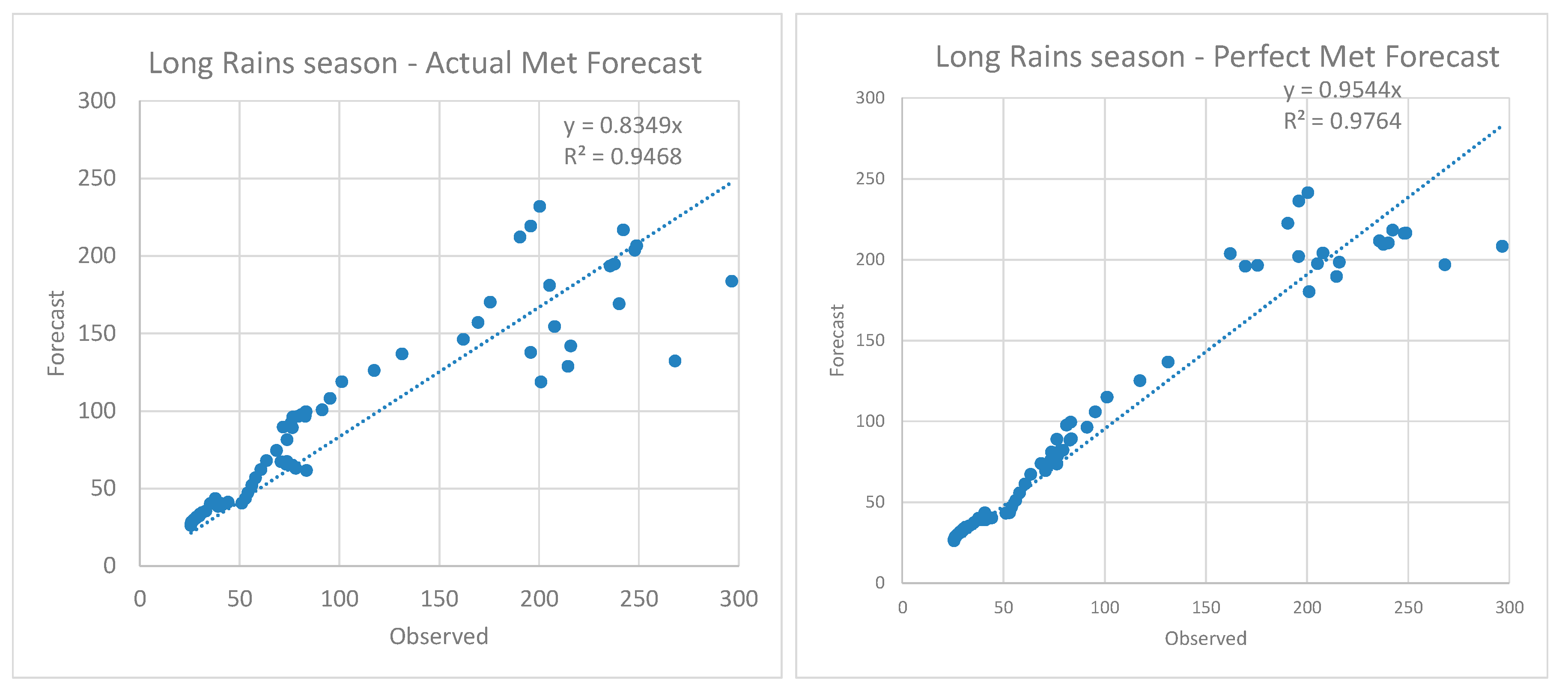

Table 1.
etadata for precipitation-gauging stations in a regular monitoring network.
| SN | Station | Code | Geographic Location | Validity period | Record Length |
% Missing | |||
|---|---|---|---|---|---|---|---|---|---|
| Latitude | Longitude | Start | End | Thiessen Area (%) | |||||
| 1 | Mlali | 9637051 | -6.9662 | 37.536 | 01/01/1956 | 31/12/2023 | 23831 | 4.1 | 1 |
| 2 | Morogoro Water Department (Morogoro Maji) | 9637052 | -6.81755 | 37.6604 | 01/01/1956 | 31/12/2023 | 24191 | 0.03 | 11 |
| 3 | Kwandewa Masa (Mongwe) | 9637049 | -6.97 | 37.58 | 31/12/1959 | 31/12/2023 | 22171 | 5.2 | 0 |
| 4 | Morning Side Farm (Morning Side Juu) | 9637046 | -6.9 | 37.67 | 01/01/1966 | 31/12/2023 | 20864 | 1.5 | 2 |
| 5 | Mondo | 9637045 | -6.95 | 37.63 | 01/01/1970 | 31/12/2023 | 19723 | 2.2 | 1 |
| 6 | Hobwe | 9637047 | -6.98 | 37.57 | 01/02/1971 | 31/12/2023 | 19047 | 1.6 | 0 |
| 7 | Ruhungo | 9637048 | -6.92 | 37.63 | 01/01/1971 | 31/12/2023 | 19292 | 0.3 | 0 |
| 8 | Matombo Mission (Matombo Primary School) | 9737006 | -7.08 | 37.77 | 01/01/1971 | 31/12/2023 | 17277 | 10.8 | 12 |
| 9 | Kibungo juu at Kibungo juu Sec. School | 9737024 | -7.07273 | 37.6882 | 01/01/1973 | 31/12/2023 | 11466 | 0 | 2 |
| 10 | Nghesse (Utari Bridge) | 9738009 | -6.99209 | 38.2906 | 01/03/2005 | 31/12/2023 | 5353 | 22.9 | 34 |
| 11 | Mindu Dam | 9637057 | -6.86285 | 37.6195 | 01/01/2009 | 31/12/2023 | 5478 | 0 | 1 |
| 12 | Ruvu at Morogoro Rd. Br | 9638029 | -6.69013 | 38.6953 | 01/01/2013 | 31/12/2023 | 4017 | 0 | 12 |
| 13 | Langali Sec. at Mgeta | 9737044 | -7.05928 | 37.5746 | 01/01/2013 | 31/12/2023 | 4017 | 1.2 | 4 |
| 14 | Milengwelengwe Met. At Mngazi | 9737029 | -7.4348 | 37.6334 | 05/02/2013 | 31/12/2023 | 3982 | 0.9 | 21 |
Table 2.
Metadata for selected flow gauging stations in a regular monitoring network.
| SN | Station | Code | Geographic Location | Networkdensity [23]** | Rating curve validity period | No. of flow gaugings | Reliability | Remarks | ||
|---|---|---|---|---|---|---|---|---|---|---|
| Latitude | Longitude | Start | End | |||||||
| 1 | Ruvu at Kidunda | 1H3 | -7.26395 | 38.24558 | 5(S) | 1993 | 2020 | 19 | Reliable | Recently demolished by flood waters of 29th April, 2024. Revitalization is going on. |
| 2 | Ruvu at Kibungo | 1H5 | -7.0237 | 37.80948 | 1(S)S | 2013 | 2021 | 45 | Unreliable | Recalibration recommended. |
| 3 | Ruvu at Morogoro Road Bridge | 1H8A | -6.6908 | 38.69427 | 7(S) | 2004 | 2020 | 79 | Unreliable | Underestimated recent (2023-2024) low flows and peak discharges. Recalibration recommended |
| 4 | Mvuha at Ngagama | 1HC2 | -7.19999 | 37.83795 | 1(S) | 2007 | 2021 | 16 | Unreliable | Recalibration recommended |
| 5 | Mgeta at Dhutumi | 1HB5 | -7.41009 | 37.77803 | 1(S) | Not published | ||||
Note: **The network densities for streamflows were assessed based on recommended minimum densities as stipulated in [23]. For the Ruvu River catchment, coastal, interior plains, and hilly/undulating regions, a minimum drainage area of 2,750 km2 was considered satisfactory (S), otherwise unsatisfactory (US).
Table 3.
Some important runoff data for the 1H3 and 1H8A catchments .
| Catchment | Area, km2 | Average flow 2013-2017, m3/s | Specific runoff l/(s*km2) | % of total flow at 1H8A (%) |
|---|---|---|---|---|
| 1H3 Kidunda | 6665 | 47.96 | 7.2 | 94 |
| 1H8A Ruvu (local) | 7696 | 3.30 | 0.4 | 6 |
| 1H8A Ruvu (total) | 14361 | 51.26 | 3.6 | 100 |
Table 4.
Metadata for TAHMO automatic weather stations in Ruvu catchment as of July 2025 (Sourced from WRBWBB database).
Table 4.
Metadata for TAHMO automatic weather stations in Ruvu catchment as of July 2025 (Sourced from WRBWBB database).
| SN | Station | Code | Geographic Location | Elevation (masl) | Validity period | Record Length |
% Missing | ||
|---|---|---|---|---|---|---|---|---|---|
| Latitude | Longitude | Start | End | ||||||
| 1. | Kibungo Juu | TA00591 | -7.07045 |
37.68955 |
1011.6 |
17/12/2018 |
08/02/2023 |
1515 |
37.8 |
| 2. | Langali Sec School | TA00592 | -7.05928 | 37.57457 | 1099 | 06/12/2018 | 17/07/2025 | 2416 |
23.6 |
| 3. | Ngerengere Utali | TA00594 | -6.99181 | 38.29105 | 114.9 |
16/12/2018 | 17/07/2025 |
2406 |
0.12 |
| 4. | Matombo primary school | TA00792 | -7.05311 | 37.76501 | 275.2 | 10/02/2023 | 17/07/2025 |
889 | 20.6 |
| 5. | Milengwelengwe secondary school | TA00793 | -7.43684 | 37.63421 | 161.6 | 10/02/2023 | 17/07/2025 |
889 |
23.2 |
|
Nash-Sutcliff Efficiency |
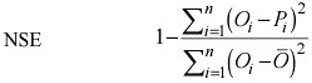 |
Range: 0 to 1 Optimal value: 1 |
|---|---|---|
|
Pearson correlation coefficient |
 |
Range -1 to 1 Optimal value: +1 (or -1) |
| Coefficient of determination R2 or R2 |
R2 = r2 |
Range 0 to 1 Optimal value: 1 |
|
Error in average flow (water balance) |
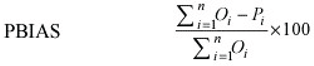 |
Optimal value: 0 |
|
Standard deviation ratio RSR |
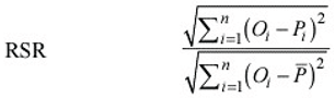 |
Range 0 to ∞ Optimal value 0 |
|
Kling-Gupta efficiency KGE |
 α is the variability of prediction errors α is the variability of prediction errors β is a bias term. |
0 to 1 Optimal value 1 |

Table 7.
Optimized HBV-model parameters for 1H8A Ruvu at Morogoro Roadbridge.
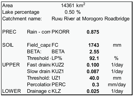 |
Table 8.
Result of HBV-model calibration and verification for 1H8A Ruvu at Morogoro Roadbridge.
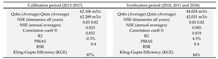 |
Table 9.
Optimized HBV-model parameters for 1H3 Kidunda.
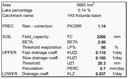 |
Table 10.
Result of HBV-model calibration and verification for 1H3 Kidunda.
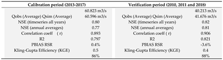 |
Table 11.
Summary statistics for Ruvu-HBV forecast skills in hydrological year 2024/25.
| Season → | Dry | Short Rains | Long Rains | All year | |||
|---|---|---|---|---|---|---|---|
| # of forecast days | 70 | 90 | 67 | 227 | |||
| Met Forecast | |||||||
| R2 | 0.964 | 0.889 | 0.947 | 0.933 | |||
| PBIAS | 0.953 | 0.812 | 0.834 | 0.866 | |||
| "Perfect" Forecast | |||||||
| R2 | 0.981 | 0.928 | 0.976 | 0.962 | |||
| PBIAS | 0.993 | 0.914 | 0.954 | 0.954 | |||
| Improvement (r2) | 0.017 | 0.039 | 0.029 | 0.028 | |||
Disclaimer/Publisher’s Note: The statements, opinions and data contained in all publications are solely those of the individual author(s) and contributor(s) and not of MDPI and/or the editor(s). MDPI and/or the editor(s) disclaim responsibility for any injury to people or property resulting from any ideas, methods, instructions or products referred to in the content. |
© 2025 by the authors. Licensee MDPI, Basel, Switzerland. This article is an open access article distributed under the terms and conditions of the Creative Commons Attribution (CC BY) license (http://creativecommons.org/licenses/by/4.0/).
Copyright: This open access article is published under a Creative Commons CC BY 4.0 license, which permit the free download, distribution, and reuse, provided that the author and preprint are cited in any reuse.


