
Submitted:
16 September 2025
Posted:
18 September 2025
You are already at the latest version
Abstract
In this paper, we deal with Stirling’s approximation to N!. We employ elementary mathematical techniques to provide an algorithm to quickly calculate many terms of Stirling’s formula remainder.
Keywords:
stirling formula
; remainder
; approximation
MSC: 41A80; 68W30
1. Introduction
In this note, we study Stirling’s approximation to , a fundamental result in asymptotic analysis and number theory. Originally derived in the 18th century, the approximation provides an accurate estimate of the factorial function for large values of N. Over the centuries, various forms and refinements of this approximation have been developed. A particularly elegant and instructive derivation, based solely on elementary transformations of integrals and term-by-term integration of a series, was introduced by Marsaglia [1].
Our first objective is to briefly derive Stirling’s formula. We begin with the representation of as a sum of logarithms:
where each term measures the discrepancy between the trapezoidal rule and the exact integral of over the interval . That is,
The integral in (1) can be evaluated explicitly,
is a telescoping sum, as the terms cancel pairwise. In this way,
which leads to
where is given in (2).
It is well known, from the Mercator series, that
Substituting , where , yields
Thus, in (2) can be rewritten as
where , for , is a positive decreasing sequence of real numbers that converges to zero.
Thus,
From the Riemann Zeta function (see [2] for details),
which is convergent for with , it follows that
and, therefore,
Additionally, from [3,4], based on the Riemann Zeta function and Rational Zeta series, it follows that
Moreover, using the Mercator series evaluated at ,
we arrive at the Suryanarayana formula (see [3] for example),
and, consequently,
In this way,
Therefore,
where is given by
and, as before, , for , is a positive decreasing sequence of real numbers that converges to zero.
Finally, Eq. (3), known in the literature as Stirling’s formula, can be expressed as
where the remainder is given in (4).
Eq (5) was first presented in [5], where it was also established that . Since then, the term has been the subject of detailed study (see [6,7,8,9] for historical notes), particularly through works such as [10], who first provided sharp two-sided bounds for it,
Several years later, [11] improved the estimation of ,
More recently, [12] obtained the following result,
[8] proved that
with the best possible constants and , and [9] derived the following inequality:
It is also important to highlight the works [1,7,13,14,15] who focused on obtaining explicit formulas for the coefficients of the asymptotic expansion of .
The main goal of this work is to present an algorithm, relying only on elementary mathematical methods techniques, for efficiently calculating many terms of exactly. To the best of our knowledge, we understand that our algorithm represents an alternative to the procedures presented herein.
2. The Algorithm
Observe that in (4) can be rewritten as
a numerical series whose general term forms a convergent alternating series for each N. Define
the sequence of partial sums of this series.
Step 1: Consider the polynomial defined by the following equation:
where is a real parameter to be determined later. This leads to:
Now, is chosen in order to reduce the degree of to the lowest possible value. In this case, and, after some calculations, we obtain
which is a polynomial of degree 1, that is, . We denote by the coefficient associated with the highest degree term of the polynomial .
In this way, the partial sum can be expressed as
As an important remark, in (4) can then be approximated by
The sum above can be estimated using the integral test, comparing it to an improper integral.
Step 2: Similarly, we seek a polynomial that satisfies
where is a real parameter to be determined.
Thus,
Again, is chosen with the aim of reducing the degree of to the lowest possible value. In this case, .
Therefore, we can present as
where
Note that and .
Again, as a remark, in (4) is better approximated by
Step 3: Similarly, aiming for a better approximation of , we write
where is, as before, a real parameter to be determined.
The polynomial can be rewritten as
The parameter is chosen with the aim of reducing the degree of to the lowest possible value. Thus, .
Then, is given by
where
Note that and .
Therefore, a better approximation for in (4) is obtained:
Step 4: Likewise, the polynomial is defined as
Taking , we obtain
where and .
Thus,
and then
where .
In summary, the following algorithm is presented.
Step 5: Algorithm
Remark 1.
The sequence , for , defined above, is crucial because it leads to
Furthermore, based on computational tests, it was observed that, for ,
The exact calculations of and , for , were carried out using symbolic computations in the Mathematica software [16], using the script that follows:
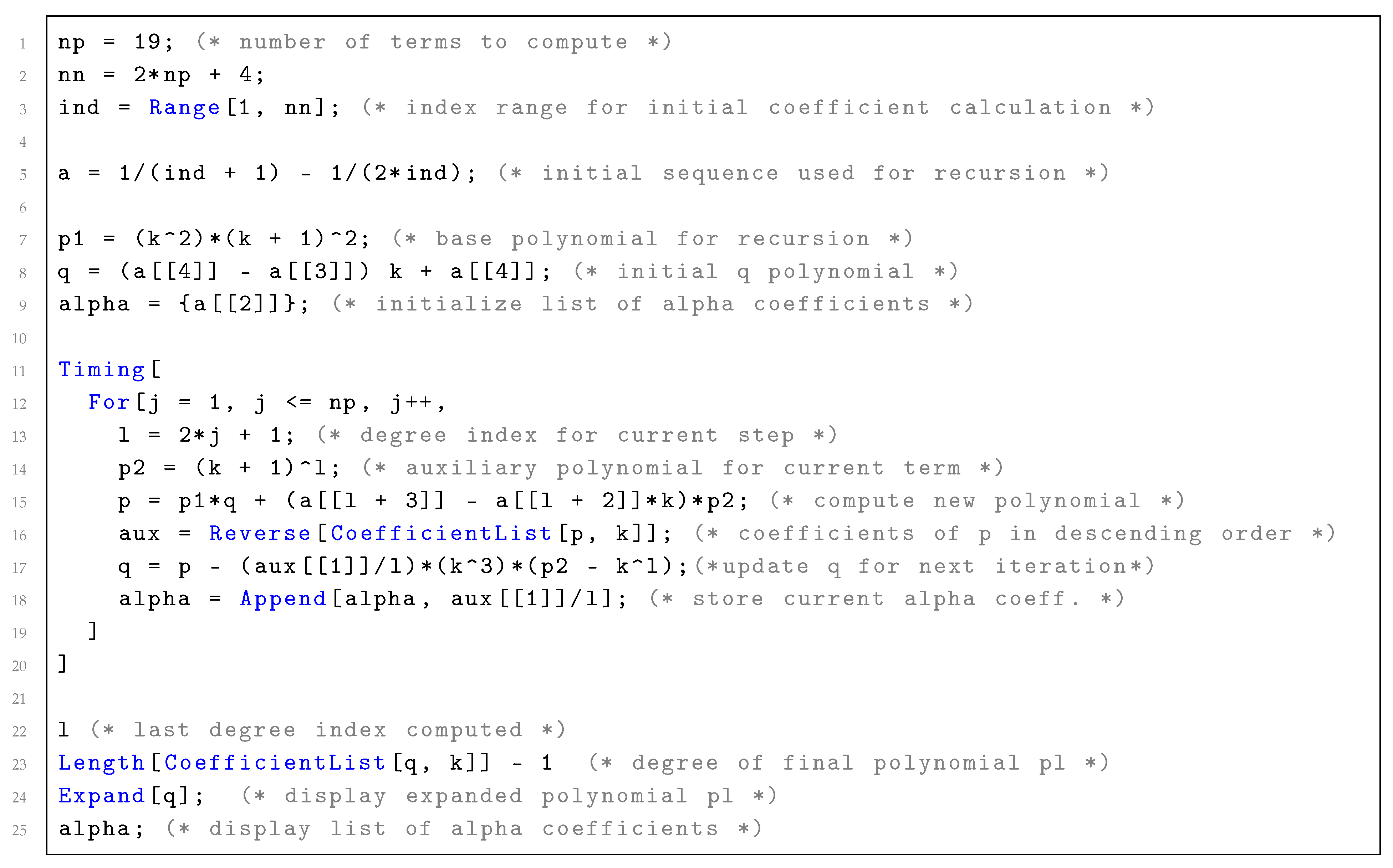
To illustrate our algorithm, we calculate using the Mathematica script provided above (CPU time approximately seconds, executed in the trial version of Mathematica Online) and then, in (4) can be approximated by
As a test, the CPU time to calculate the first 300 terms of was approximately 200 seconds. Remark 1 have been verified in this case.
References
- Marsaglia, G., Marsaglia, J.C.W.: A new derivation of stirling’s approximation to n! Am. Math. Mon. 97:9, 826–829 (1990).
- Lagarias, J.C.: Euler’s constant: Euler’s work and modern developments. Bulletin of the American Mathematical Society 50(4), 527–628 (2013).
- Coppo, M.-A.: A note on some alternating series involving zeta and multiple zeta values. Journal of Mathematical Analysis and Applications 475(2), 1831–1841 (2019).
- Borwein, J.M., Bradley, D.M., Crandall, R.E.: Computational strategies for the riemann zeta function. Journal of Computational and Applied Mathematics 121(1), 247–296 (2000).
- Hummel, P.M.: A note on stirling’s formula. Am. Math. Mon. 47, 97–99 (1940).
- Beesack, P.R.: Improvement of stirling’s formula by elementary methods. Univ. Beograd. Publ. Elektrotehn. Fak. Set. Mat. Fiz. 274-301, 17–21 (1969).
- Nemes, G.: On the coefficients of the asymptotic expansion of n! (2010). https://arxiv.org/abs/1003.2907.
- Chen, C.P., Batir, N.: Some inequalities and monotonicity properties associated with the gamma and psi functions. Appl. Math. Comput. 218, 8217–8225 (2012).
- Lin, L.: On stirling’s formula remainder. Applied Mathematics and Computation 247, 494–500 (2014).
- Nanjundiah, T.S.: Note on stirling’s formula. Am. Math. Mon. 66, 701–703 (1959).
- Robbins, H.: A remark on stirling’s formula. Am. Math. Mon. 62, 26–29 (1955).
- Shi, X., Liu, F., M., H.: A new asymptotic series for the gamma function. J. Comput. Appl. Math. 195, 134–154 (2006).
- Comtet, L.: Advanced Combinatorics: The Art of Finite and Infinite Expansions - Stirling Numbers, pp. 204–229. Springer, Dordrecht (1974). [CrossRef]
- S., B., M´endez, A.: The asymptotic expansion for n! and Lagrange inversion formula (2010). https://arxiv.org/abs/1002.3894.
- Impens, C.: Stirling’s series made easy. Am. Math. Mon. 110:8, 730–735 (2003).
- Inc., W.R.: Mathematica Online, Version 14.2. Champaign, IL, 2024. https://www.wolfram.com/mathematica.
Disclaimer/Publisher’s Note: The statements, opinions and data contained in all publications are solely those of the individual author(s) and contributor(s) and not of MDPI and/or the editor(s). MDPI and/or the editor(s) disclaim responsibility for any injury to people or property resulting from any ideas, methods, instructions or products referred to in the content. |
© 2025 by the authors. Licensee MDPI, Basel, Switzerland. This article is an open access article distributed under the terms and conditions of the Creative Commons Attribution (CC BY) license (http://creativecommons.org/licenses/by/4.0/).
Copyright: This open access article is published under a Creative Commons CC BY 4.0 license, which permit the free download, distribution, and reuse, provided that the author and preprint are cited in any reuse.


