Submitted:
01 September 2025
Posted:
02 September 2025
You are already at the latest version
Abstract
The deployment of traditional ground-penetrating radar (GPR) systems for ice detection on steep terrain presents substantial safety challenges for ground crews due to inaccessi-bility and hazardous working conditions. However, airborne GPR (AGPR) and radio echo sounding (RES) provide solutions for these difficulties. Assuming ice is homogeneous, we introduce a perspective back-projection algorithm designed to process AGPR or RES data that directly searches for unobstructed refracted electromagnetic (EM) wave paths and fo-cusing EM energy below the surface by computing path-specific travel times. Our results from 2-D and 3-D imaging tests indicate that the perspective back-projection algorithm can accurately image the ice-rock interface. However, Snell's Law suggests that part of the energy may fail to propagate through the air-ice interface and reach either the ice-rock in-terface or the receivers in scenarios where the incident angle of an EM wave exceeds a cer-tain threshold. This energy deficit can hinder the perspective back-projection algorithm from accurately imaging such ice-rock interfaces. Despite these limitations, the perspective back-projection algorithm remains a promising tool for imaging sub-ice interfaces in AGPR and RES ice detection.
Keywords:
ice detection
; airborne ground-penetrating radar
; radio echo sounding
; interface imaging
1. Introduction
Significant transformations in water resources have significantly impacted Earth's ecosystems [1,2]. Ice detection [3] encompassing the examination of ice thickness plays a crucial role in freshwater studies [4,5], along with the monitoring of ice deformation [6], and the analysis of physical and chemical properties of ice [7-10]. Ground-penetrating radar (GPR) [11-13] technology has emerged as a highly effective geophysical technique for ice thickness surveying. Meanwhile airborne ground-penetrating radar (AGPR) [14-16] systems, utilizing advanced GPR technology on aerial platforms, significantly expanded operational reach and enabled the surveying of areas that were previously inaccessible. This system has several advantages, including exceptional efficiency, high resolution, and non-intrusiveness, making it highly applicable in various fields. However, complexities arising from factors such as interfacial fluctuations [17] pose challenges to the effective utilization of AGPR.
In geophysical applications, reverse-time migration (RTM) [18] techniques are widely used for the data processing of seismic data, to correct imaging distortions of interfaces. RTM is based on the numerical simulations for the propagation of EM waves. In this process, received signals are retrogradely propagated at half the wave speed back into the subsurface medium. In GPR explorations [19-21], RTM technology ensures that the EM energy is accurately focused at the underground reflection points, reducing imaging distortions caused by medium heterogeneity and interfacial undulations. However, when applying RTM to the processing of large-scale airborne or spaceborne GPR glacier detection, long profiles or extensive areas with depths are assessed, which demand significant computational resources and introduce challenges for the practical application of RTM in solid water resource surveys and related fields.
Radar systems mounted on satellites or aerial platforms play a critical role in ice detection, due to their high efficiency and penetrative power [22-25]. The back-projection (BP) algorithm [26,27], known for its high-precision imaging capabilities in radar data processing, utilizes the time-delay information of radar signals to project scattered signals back to their origins, thus achieving signal focusing. Unlike the classical RTM (CRTM) algorithm [18], the classical BP (CBP) algorithm [28] can efficiently focus energy by directly calculating the travel times of waves, eliminating the need for the forward modeling of wave propagation. Moreover, because the focusing calculation at each grid node operates independently, the CBP algorithm can achieve parallel computation, allowing it to be used for detection tasks in homogeneous media. In non-homogeneous cases, such as air-ice-rock model, refraction may occur [27]. Consequently, because EM waves with relatively low frequencies can penetrate ice to considerable depths, potentially reaching thousands of meters, directly applying the CBP algorithm to ice detection data, without accounting for the effects of refraction, may result in inaccuracies in determining the wave travel paths. These inaccuracies may ultimately manifest as false anomalies within the imaging results.
Researchers [27,29] have applied the modified 2-D BP algorithm to the processing of AGPR data. However, techniques for calculating refraction paths in both algorithms have been developed based on the geometric assumptions of horizontal medium surfaces and thus they cannot be applied to scenarios involving undulating terrain surfaces. Specifically, the refraction point estimation method used in the algorithm developed by Qu et al. was designed for applications with a refractive index greater than or equal to 1, without accounting for total reflection conditions. Another imaging algorithm [30] also based on BP was developed for synthetic aperture radar (SAR) data to estimate glacier volume. For the same application in AGPR or radio echo sounding (RES) field exploration scenarios, this study proposed a perspective back-projection (PBP) algorithm. The PBP framework has two key characteristics: 1) 2-D and 3-D imaging capability for AGPR and RES data; 2) the systematic detection of propagation path occlusions within the computational workflow. These advancements collectively enabled 2-D and 3-D subsurface imaging through the comprehensive integration of surface geomorphological constraints. These factors established PBP as a suitable sub-interface imaging methodology for AGPR and RES exploration.
In this study, we first introduced the CRTM and CBP algorithms, and then described the key steps of our proposed PBP algorithm. Subsequently, we described several 2-D and 3-D air-ice-rock models and their corresponding EM forward modeling (FWD) results, and compared the imaging profiles generated by the CRTM and PBP algorithms. Finally, we discussed the performance of PBP algorithm through additional numerical experiments and provided conclusions regarding its effectiveness.
2. Materials and Methods
2.1. General Scheme
To address ice-rock interface imaging challenges, in this work, we developed the perspective back-projection (PBP) algorithm by integrating fundamental principles from the classical reverse-time migration (CRTM) method and core strategies from the classical back-projection (CBP) technique. For methodological clarity, we first introduced the essential concepts underlying CRTM and CBP before detailing the PBP framework.
Various RTM algorithms have been leveraged in seismic exploration to image subsurface interfaces [18]. Due to the high degree of similarity between the foundational principles of GPR application and seismic exploration, RTM algorithms have also been successfully adapted for use in GPR applications. The fundamental imaging theorem for the RTM in GPR was introduced as follows: Neglecting the effects of complex propagation paths and the influence of multiple scattered waves, the travel time of the emitted EM waves to the scatterer will be approximately equal to that of the scattered signals to the receiving antenna. According to this principle, if the signals received by the receiving antenna are transmitted backward at half the phase velocity, the EM energy could be accurately concentrated at the scatter and interface locations, thereby achieving imaging.
Compared to the RTM algorithms, the CBP algorithm has been widely used in synthetic aperture radar (SAR) imaging. Grounded in the principles of EM wave propagation in homogeneous media, the core steps of the CBP algorithm involve calculating the accurate time delay of scattering and projecting the corresponding echo signals into the imaging plane, which fundamentally aligns with the back-propagating echo signals to the scattering/reflecting points in the RTM algorithms. CBP implementation comprises: (1) computing time delays for all transmitter-receiver pairs relative to a given node in the mesh grid (i.e., a media interface node) and (2) performing the weighted summation of delay-corresponding echoes to reconstruct an image of the scatter.
The PBP algorithm shared most fundamental steps with the CBP algorithm, however, it incorporated modifications in time delay computation. The application of the PBP algorithm in ice exploration could be predicated on several key assumptions. (a) When EM waves traverse different media, their paths will be subjected to refraction. (b) For simplicity, ice could be treated as a homogeneous medium in the air-ice-rock model. (c) Propagation within bedrock could be disregarded, given the limited penetration depth of the signal.
Assumption (a) implied that the travel paths found by the PBP algorithm more closely approximated real-world cases than those from the CBP algorithm. Meanwhile, assumptions (b) and (c) enabled the simplification of the travel path calculations by confining refraction computations to a homogeneous ice medium.
Considering the aforementioned assumptions, the principal steps for the PBP algorithm are delineated as follows:
(1) The air-ice interface was discretized and the algorithm searched for the valid refraction point corresponding to each transmitting-receiving pair. The criteria for determining valid refraction points will be provided later.
(2) The coordinates of the refraction points, transmitters, and receivers were used to determine the travel paths for refractions and backscatterings.
(3) The validity of the travel paths (as shown in Figure 1) was determined. If an incident path intersected the air-ice interface at any location(s) except for the refraction point, it was deemed invalid. If a transmitted path intersected the air-ice interface at any location(s) except for the refraction point, only the segment between the refraction point and the nearest intersecting point was considered valid.
(4) The physical parameters of air and ice could be employed to compute the two-way travel time for each travel path.
(5) The travel times could be used to select the appropriate EM field components after pulse-compression processing and these components could be summed to focus the energy onto the mesh grid.
(6) Steps (1) through (5) can be iteratively executed for every node in the mesh grid.
2.2. Construction of the Air-Ice Model
Based on assumptions (b) and (c) mentioned above, the PBP algorithm did not account for rock. Thus, two-layer model (air-ice model) was used for practical ice surveys. Within this framework, the air and homogeneous ice were separated by the air-ice interface, where refraction occurred. Consequently, travel paths and travel times were calculated within the domains of air and homogeneous ice.
2.3. Identification of Valid Refraction Point
Prior to identification, it was essential to define the concept of a valid refraction point. In this study, a valid refraction point referred to a point that, along with the transmitter and receiver, determined the reasonable incident, refracted, and reflected paths that were consistent with the classical electrodynamics. The validity of a refraction point was maintained by following fundamental principles derived from electrodynamics. Assuming that the refractive index of ice was n, the following inequalities and conditions had to be satisfied:
(a) cos(θi)>0 and cos(θr)>0, where θi and θr denote the incidence and refraction angles (Figure 2), respectively.
(b) In general, the incidence and refraction path had to be separated by a line, which coincided with the normal vector at the refraction point on the air-ice interface.
(c) The sine values of the angles determined by Snell’s Law had to be less than or equal to one.
(d) Specifically, if the incidence and refraction paths determined by the current refraction point were both collinear with the normal vector at the refraction point, then the current refraction point was also deemed valid.
(e) Except for the intersection at the refraction point, no other intersections could be present between the paths and the air-ice interface. Otherwise, the refraction point would be deemed invalid.
(f) In general cases, it could be possible to encounter multiple valid refraction points for a specific transmitter, receiver, and scattering node combination. Consequently, the PBP algorithm often handled instances of multiple refractions.
(g) A refraction point associated with an invalid incident path was considered invalid.
2.4. Determination of the Travel Path
Once refraction points were determined, the spatial coordinates of the associated transmitters, receivers, and scattering points could be combined to derive the travel paths. Based on known or assumed electrical properties of the media, the travel times for each path could be subsequently determined.
To simplify the analysis in this study, two further simplifications were introduced. First, we assumed that for any given transmission-reception event, the transmitter and receiver shared the same antenna. Second, we hypothesized that the forward and reverse propagation signals followed identical travel paths.
2.5. Mesh Grid for Imaging
The PBP algorithm differed from the CRTM algorithm in how it handled the imaging mesh grid. Theoretically, the PBP algorithm can perform computations on uniformly partitioned or non-uniformly partitioned grids of any density. According to the computation steps mentioned above, the PBP algorithm was insensitive to the mesh grid density, allowing it to handle both sparse and dense grids without compromising computational stability. This flexibility was especially advantageous for long-distance profiling tasks spanning tens to hundreds of kilometers or 3-D imaging tasks for large area.
3. Results
In this section, we conducted the FWDs of synthetic air-ice-rock 2-D and 3-D models to provide input data for the CRTM and PBP algorithms. Then, the resulting imaging profiles from these algorithms were depicted and compared. The FWD algorithm was based on the finite-difference time-domain (FDTD) method [31] and the convolutional perfectly matched layer (CPML) technique [32].
The EM properties of air, ice, and rock used in this study for the synthetic tests are detailed in Table 1. To maintain numerical stability and make sure that the signal was sampled accurately in space, the time step had to satisfy the Courant-Friedrichs-Lewy (CFL) condition [33], where the grid step was not larger than a fraction of the highest-frequency wavelength. For a reasonable FDTD simulation, setting the highest-frequency wavelength larger than 20 cells size was sufficient [31]. The central frequency of the electromagnetic wave signal used in the simulation experiments of this study was 900 MHz (signal was shown in the next section). To sufficiently suppress numerical dispersion and minimize the impact of computational errors on the imaging results, the time step and grid step were set as 4.1461×10⁻¹² s and 2-9 m respectively for all 2-D computations, while for the 3-D simulations, the values were 3.3853×10⁻¹² s and 2-9 m.
3.1. Signal
The Blackman-Harris window, a versatile windowing function, has been widely used for signal processing and spectral analysis [34,35]. In this study, the derivative of the Blackman-Harris window function (the central frequency was 900 MHz, as shown in Figure 3) served as the electric current source in the forward modeling of AGPR exploration. Notably, our decision to use this function as the current source was not driven by any specific theoretical or empirical justification. In addition, a single antenna was used for both transmission and reception.
3.2. 2-D Model Tests
In this work, we performed four 2-D imaging tests. First, as shown in Figure 4a, we constructed a 2-D model designated as Model-2D-HAI-SIG, characterized by a horizontal air-ice interface and an approximately stepped ice-rock interface. The model dimensions were 6 m in the x-direction and 3 m in the z-direction, yielding 3072 cells along the x-direction and 1536 cells along the z-direction. The curve to determine the ice-rock interface utilized the following form:
The transmitters were positioned on the green line in Figure 4a, each 1.0 m above the peak elevation of the air-ice interface. We established 337 transmitter points in total, performing 337 2-D FWD computations to construct the received signal profile, as shown in Figure 4b. The imaging results of CRTM and PBP are shown in Figure 4c and 4d, respectively. Both algorithms successfully reconstructed the ice-rock interface, though with lower energy focus at the steeply inclined part of the interface compared to the horizontal ones.
As shown in Figure 5a, we constructed a 2-D model designated as Model-2D-SAI-HIG, characterized by an approximately stepped air-ice interface and a horizontal ice-rock interface. The model dimensions were 4 m in the x-direction and the z-direction, yielding 2048 cells along both the x-direction and the z-direction. The curve to determine the ice-rock interface utilized the following form:
where h was the vertical coordinate of the air-ice interface, and x was the horizontal coordinate. The transmitters were positioned on the green line in Figure 5a, one meter above the peak elevation of the air-ice interface. We had set up 225 transmitter points for this test, resulting in 225 two-dimensional FWD computations to construct the received signal (Ey) profile, as shown in Figure 5b.
The imaging results of the CRTM and PBP algorithms were shown in Figure 5c and 5d. The CRTM and PBP algorithm successfully identified the undulating air-ice interface. The results from the CRTM and PBP algorithms show obvious energy focusing on the interface between ice and rock. Notably, the rapid undulation of the air-ice interface in the central region of the model, similar to the effects of convex and concave lenses, can potentially diverge or focus the electromagnetic field, and eventually affect the energy focusing. Although, this effect may have contributed to the analogous low-energy focusing phenomena observed in the regions immediately beneath the rapidly undulating air-ice interface region in Figure 5c and 5d, the results support the effectiveness of the PBP algorithm in models such as Model-2D-SAI-HIG, which are characterized by undulating air-ice interfaces and horizontal ice-rock interfaces.
To validate the PBP algorithm in a more complex scenario, we subsequently constructed another 2-D synthetic model, designated as Model-2D-SAI-SIG (Figure 6a), which featured approximately stepped ice-rock and air-ice interfaces. The model dimensions were 4 m in the x-direction and 3.5 m in the z-direction. Consequently, we achieved 2048 cells along the x-direction and 1792 cells along the z-direction. The equations for the air-ice interface and ice-rock interface could be obtained by:
The transmitters were positioned along the green line in Figure 6a and placed 1.0 m above the peak elevation of the air-ice interface. We also established 225 transmitter points. The received signal (Ey) profile is depicted in Figure 6b.
Figure 6c and 5d presents the imaging results obtained from the CRTM and PBP algorithms. Both algorithms achieved energy focusing on the ice-rock interface but exhibited a limited resolution on the steeply inclined interface segments in this test.
Ice fractures are a common occurrence. To evaluate the performance of the PBP algorithm in detecting such fractures, we created a synthetic model, as shown in Figure 7a, named the Model-2D-HAI-HIG-F. This model was designed with horizontal air-ice and ice-rock interfaces, and it incorporated ice fractures within the ice layer, providing a controlled scenario to test the algorithm's fracture detection capabilities. The model dimensions were 4 meters in the x-direction and 3 meters in the z-direction. Accordingly, the model comprised 2048 cells along the x-direction and 1536 cells along the z-direction. There were three fractures in this model. The horizontal fracture was named F1, the tilted fracture F2, and the vertical fracture F3. The F1 was set by the equations below:
The F2 took the form:
The F3 took the form:
The transmitters were located along the green line in Figure 7a, one meter above the air-ice interface. We had set up 225 transmitter points and illustrated the profile of the received signals (Ey) in Figure 7b.
Figure 7c and 7d showed the imaging results from the CRTM and PBP algorithms. Both the CRTM and PBP algorithms could accurately recover the ice-rock interface and the gently inclined fractures. However, when it comes to the vertical fracture, neither the CRTM nor the PBP algorithm could provide obvious imaging results in this test.
3.3. 3-D Model Test
We also constructed a 3-D synthetic model, designated as Model-3D-HAI-SIG (Figure 8a), to validate our algorithm's performance under the 3-D condition. To achieve balance among the validation requirements of the PBP algorithm, computational costs, and numerical stability of FWD, this 3-D model featured a slightly depressed ice-rock interface, a horizontal air-ice interface, and a compact size in all dimensions. The model dimensions were 0.6 m in the x-direction, 0.4 m in the y-direction, and 1 m in the z-direction. The model was discretized into 308 cells along the x-direction, 205 cells along the y-direction, and 513 cells along the z-direction. The ice-rock interface geometry was defined by the following equations:
We established 1763 transmitter points 0.4 m above the peak elevation of the air-ice interface. These points were marked by blue dots in Figure 8a. The received Ey-component signal slices are shown in Figure 8b.
The imaging results obtained from the CRTM and PBP algorithms are presented in Figure 8c and 6d, respectively. Both algorithms successfully revealed the ice-rock interface.
4. Discussion
Backscattering refers to a phenomenon where waves, such as EM or sound waves, encounter obstacles or medium inhomogeneities during propagation, causing some of the energy to be reflected or scattered back toward the wave source. The PBP algorithm proposed in this work was an imaging algorithm that solely utilized backscattering signals to achieve EM wave energy focusing. Previous studies [36,37] found that: (1) the energy intensity of backscattered signals varied with the incident angle, and (2) a strong backscattered signal was generated when EM waves were incident perpendicular to a material interface. The 2-D imaging results on the synthetic model demonstrated degraded performance at steeply inclined ice-rock interfaces. This limitation stemmed from the combined influence of interface geometries (both air-ice and ice-rock) and the physical properties of the icy medium, together preventing the EM waves from achieving normal incidence at steeply inclined ice-rock interfaces. As a result, strong vertically backscattered signals could not be acquired from the steeply inclined interface, leading to the PBP algorithm's impaired imaging capability. To validate the above hypothesis, this study employed Snell's Law and geometric analysis to analytically determine the specific locations along the ice-rock interface in the electrical model of the Model-2D-HAI-SIG capable of producing strong backscattering, as well as the corresponding time instances in the B-SCAN profile exhibiting intense backscattering signals. Figure 9 explained the basic strategy for determining the specific locations along the ice-rock interface, which were capable of producing strong backscattering. TR represented the transmitting/receiving antenna; gai denoted arbitrary discrete grid nodes on the air-ice interface; vai represents the normal vector of the air-ice interface at point gai; ptr-ai denotes the vector pointing from gai to TR. Assuming the refractive index of ice is known, the transmission direction pai-ig corresponding to all discrete nodes on the air-ice interface can be calculated with the usage of Snell’s Law, excluding all cases of total reflection.
Then, we could determine the position where pai-ig (the electromagnetic wave propagation path) intersects with the ice-ground interface, denoted as gig. At this point, the interface normal vector vig at position gig was compared with the propagation path pai-ig. If the angle θerr between them is smaller than a predefined threshold, the grid node on the ice-ground interface capable of producing strong backscattering is identified.
Knowing the identified grid node gig on the ice-ground interface capable of producing strong backscattering, along with the spatial coordinates of the corresponding gai and TR, the travel times of the electromagnetic wave propagation paths pai-ig and ptr-ai can be calculated.
These predicted positions and timings are explicitly marked by triangles in Figure 10. The analytical results demonstrated that, in this configuration, steeply inclined ice-rock interfaces could not generate significant backscattering due to the constraints imposed by Snell's Law. Conversely, echoes from gently inclined or horizontal ice-rock interfaces dominated the B-SCAN profile.
Additionally, the normal vectors of all grid nodes on the ice-ground interface are provided in Figure 11b. Given the normal vector at any point on this interface, a straightforward calculation based on Snell’s Law can determine whether electromagnetic waves propagating along the normal vector direction at any nodal location can penetrate the air-ice interface and transmit into the air. The nodes corresponding to cases where such electromagnetic waves fail to penetrate are designated as IG. In Figure 11b, the curve segments associated with IG nodes are colored red. The horizontal coordinate ranges corresponding to these red-colored curve segments are bounded by two blue dashed lines in Figure 11a and b. It could be observed that the horizontal coordinate ranges of these red-colored curve segments corresponded to those of the grid nodes that were not marked by white triangles in Figure 10a. This phenomenon implied that some parts of the grid nodes on the ice-ground interface could not generate strong backscattered signals.
To further verify that steeply inclined ice-rock interfaces in this case could not generate strong backscattering signals, we conducted an equivalent simulation experiment. In Model-2D-HAI-SIG, we densely arranged 337 radar signal transmission points along the steeply inclined ice-rock interface. This experimental design enabled the transmission of a quasi-planar EM wave approximately parallel to the steeply inclined ice-rock interface near its central region, with the propagation direction perpendicular to the interface. The inability of this plane wave to penetrate the air-ice interface constituted definitive proof that strong backscattering could not originate from the steeply inclined ice-rock interface. Six time slices are shown in Figure 12. The results demonstrated that the quasi-planar wave emitting from the central region of the steeply inclined ice-rock interface failed to penetrate the air-ice interface. Notably, the simulation results revealed that certain EM waves successfully propagated through the air-ice interface into the air. Notably, as these waves originated from transmitter locations at both marginal zones of the steeply inclined ice-rock interface, the EM fields out of these edge locations could not be treated as components of the plane waves but the EM fields from two-dimensional line sources. Thus, these phenomena did not weaken the conclusion that steeply inclined ice-rock interfaces in this case could not generate strong backscattering signals. In summary, the absence of strong backscattering from steeply inclined ice-rock interfaces likely constituted a key factor limiting the imaging performance of both CRTM and PBP methods for these interfacial structures.
5. Conclusions
Firstly, the results of imaging tests suggested that the PBP algorithm was capable of accurately determining the positions of 2-D and 3-D ice-rock interfaces.
Secondly, the CRTM algorithm, which employed the FDTD method, necessitates small time and spatial increments to ensure the stability of numerical computations and reduce numerical dispersion. In contrast, the PBP algorithm, inheriting the flexibility of the CBP algorithm, could make the mesh grid sparse to reduce computational cost while maintaining accuracy.
Thirdly, the PBP algorithm could handle some combinations of air-ice and ice-rock interfaces, but not all. This was due to the refraction introduced by the AGPR or RES detection itself. Notably, in imaging the ice-rock interface, it was not essential to ask whether the ice-rock was steeply inclined, but rather to determine whether the strong backscattering signal could propagate through the air-ice interface on the basis of Snell’s Law and ultimately be detected by the receivers.
In summary, the PBP algorithm demonstrated its reliability and effectiveness as an interface imaging tool, not only for ice detection using AGPR or RES, but also for various penetrating detection scenarios that utilize the penetration capabilities of EM signals. In the future, we will consider incorporating denoising to enhance performance.
Author Contributions
Y. W.: Conceptualization, methodology, software, validation, writing—original draft. J. Z.: Conceptualization, formal analysis, supervision. J. P.: investigation, funding acquisition. Y. L.: conceptualization, supervision, writing—review and editing. All authors have read and agreed to the published version of the manuscript.
Funding
This research was funded by the National Key Research and Development Program of China (grant number: No. 2022YFB3902600).
Data Availability Statement
Several 2-D models and forward modeling results associated with this research are available and can be accessed via the following URL: https://1drv.ms/f/c/a48d583f70de6d0d/Em__VNGISK5CmDpMFi81MqcBkMc7zEpGqNNf4T7ivYiZSw?e=W8i6A5.
Conflicts of Interest
The authors declare that they have no known competing financial interests or
personal relationships that could have appeared to influence the work reported in this paper.
Abbreviations
The following abbreviations are used in this manuscript:
| GPR | Ground-penetrating radar |
| AGPR | Airborne ground-penetrating radar |
| RES | Radio echo sounding |
| EM | Electromagnetic |
| RTM | Reverse-time migration |
| BP | Back-projection |
| CRTM | Classical reverse-time migration |
| CBP | Classical back-projection |
| SAR | Synthetic aperture radar |
| PBP | Perspective back-projection |
| FWD | Forward modeling |
| FDTD | Finite-difference time-domain |
| CPML | Convolutional perfectly matched layer |
| CFL | Courant-Friedrichs-Lewy |
References
- Feng, X., Fu, B., Piao, S., Wang, S., Ciais, P., Zeng, Z., Lü, Y., Zeng, Y., Li, Y., Jiang, X., & Wu, B. Revegetation in China’s Loess Plateau is approaching sustainable water resource limits. Nat. Clim. Chang. 2016, 6, 1019-1022. [CrossRef]
- Peng, S., Terrer, C., Smith, B., Ciais, P., Han, Q., Nan, J., Fisher, J.B., Chen, L., Deng, L., & Yu, K. Carbon restoration potential on global land under water resource constraints. Nat Water 2024, 2, 1071-1081. [CrossRef]
- Zakharov, I., Puestow, T., Khan, A.A., Briggs, R., & Barrette, P. Review of River Ice Observation and Data Analysis Technologies. Hydrology 2024, 11. [CrossRef]
- Farinotti, D., Huss, M., Fürst, J.J., Landmann, J., Machguth, H., Maussion, F., & Pandit, A. A consensus estimate for the ice thickness distribution of all glaciers on Earth. Nat. Geosci. 2019, 12, 168-173. [CrossRef]
- Millan, R., Mouginot, J., Rabatel, A., & Morlighem, M. Ice velocity and thickness of the world’s glaciers. Nat. Geosci. 2022, 15, 124-129. [CrossRef]
- Yang, Z., Xi, W., Yang, Z., Shi, Z., & Qian, T. Monitoring and Prediction of Glacier Deformation in the Meili Snow Mountain Based on InSAR Technology and GA-BP Neural Network Algorithm. Sensors 2022, 22. [CrossRef]
- Du, Z., Cui, H., Wang, L., Yan, F., Liu, Y., Xu, Q., Xie, S., Dou, T., Li, Y., Liu, P., Qin, X., & Xiao, C. Characteristics of methane and carbon dioxide in ice caves at a high-mountain glacier of China. Sci Total Environ 2024, 946, 174074. [CrossRef]
- Huber, C.J., Eichler, A., Mattea, E., Brütsch, S., Jenk, T.M., Gabrieli, J., Barbante, C., & Schwikowski, M. High-altitude glacier archives lost due to climate change-related melting. Nat. Geosci. 2024, 17, 110-113. [CrossRef]
- Radić, V., & Hock, R. Regionally differentiated contribution of mountain glaciers and ice caps to future sea-level rise. Nat Geosci 2011, 4, 91-94. [CrossRef]
- Zamora, R., Uribe, J., Oberreuter, J., & Rivera, A. Ice thickness surveys of the Southern Patagonian Ice Field using a low frequency ice penetrating radar system. 2017 First IEEE International Symposium of Geoscience and Remote Sensing (GRSS-CHILE), Valdivia, Chile, 15-16 June 2017.
- Church, G., Bauder, A., Grab, M., & Maurer, H. Ground-penetrating radar imaging reveals glacier's drainage network in 3D. The Cryosphere 2021, 15, 3975-3988. [CrossRef]
- Grab, M., Mattea, E., Bauder, A., Huss, M., Rabenstein, L., Hodel, E., Linsbauer, A., Langhammer, L., Schmid, L., Church, G., Hellmann, S., Délèze, K., Schaer, P., Lathion, P., Farinotti, D., & Maurer, H. Ice thickness distribution of all Swiss glaciers based on extended ground-penetrating radar data and glaciological modeling. J Glaciol 2021, 67, 1074-1092. [CrossRef]
- Letamendia, U., Navarro, F., & Benjumea, B. Ground-penetrating radar as a tool for determining the interface between temperate and cold ice, and snow depth: a case study for Hurd-Johnsons glaciers, Livingston Island, Antarctica. Ann Glaciol 2023, 1-9. [CrossRef]
- Fu, L., Liu, S., Liu, L., & Lei, L. Development of an Airborne Ground Penetrating Radar System: Antenna Design, Laboratory Experiment, and Numerical Simulation. Ieee J-stars 2014, 7, 761-766. [CrossRef]
- Rutishauser, A., Maurer, H., & Bauder, A. Helicopter-borne ground-penetrating radar investigations on temperate alpine glaciers: A comparison of different systems and their abilities for bedrock mapping. GEOPHYSICS 2016, 81, WA119-WA129. [CrossRef]
- Tjoelker, A.R., Baraër, M., Valence, E., Charonnat, B., Masse-Dufresne, J., Mark, B.G., & McKenzie, J.M. Drone-Based Ground-Penetrating Radar with Manual Transects for Improved Field Surveys of Buried Ice. Remote Sens 2024, 16. [CrossRef]
- Chi, Y., Mao, L., Wang, X., Pang, S., & Yang, Y. Three-dimensional numerical simulation and experimental validation of airborne ground-penetrating radar based on CNCS-FDTD method under undulating terrain conditions. Sci Rep 2024, 14, 22156. [CrossRef]
- Zhou, H.-W., Hu, H., Zou, Z., Wo, Y., & Youn, O. Reverse time migration: A prospect of seismic imaging methodology. Earth-sci Rev 2018, 179, 207-227. [CrossRef]
- Delf, R., Bingham, R.G., Curtis, A., Singh, S., Giannopoulos, A., Schwarz, B., & Borstad, C.P. Reanalysis of Polythermal Glacier Thermal Structure Using Radar Diffraction Focusing. J Geophys Res-earth 2022, 127, e2021JF006382. [CrossRef]
- Liu, H., Long, Z., Tian, B., Han, F., Fang, G., & Liu, Q.H. Two-Dimensional Reverse-Time Migration Applied to GPR With a 3-D-to-2-D Data Conversion. Ieee J-stars 2017, 10, 4313-4320. [CrossRef]
- Wang, Y., Fu, Z., Lu, X., Qin, S., Wang, H., & Wang, X. Imaging of the Internal Structure of Permafrost in the Tibetan Plateau Using Ground Penetrating Radar. Electronics 2019, 9. [CrossRef]
- Blankenship, D.D., Moussessian, A., Chapin, E., Young, D.A., Wesley Patterson, G., Plaut, J.J., Freedman, A.P., Schroeder, D.M., Grima, C., Steinbrügge, G., Soderlund, K.M., Ray, T., Richter, T.G., Jones-Wilson, L., Wolfenbarger, N.S., Scanlan, K.M., Gerekos, C., Chan, K., Seker, I., Haynes, M.S., Barr Mlinar, A.C., Bruzzone, L., Campbell, B.A., Carter, L.M., Elachi, C., Gim, Y., Hérique, A., Hussmann, H., Kofman, W., Kurth, W.S., Mastrogiuseppe, M., McKinnon, W.B., Moore, J.M., Nimmo, F., Paty, C., Plettemeier, D., Schmidt, B.E., Zolotov, M.Y., Schenk, P.M., Collins, S., Figueroa, H., Fischman, M., Tardiff, E., Berkun, A., Paller, M., Hoffman, J.P., Kurum, A., Sadowy, G.A., Wheeler, K.B., Decrossas, E., Hussein, Y., Jin, C., Boldissar, F., Chamberlain, N., Hernandez, B., Maghsoudi, E., Mihaly, J., Worel, S., Singh, V., Pak, K., Tanabe, J., Johnson, R., Ashtijou, M., Alemu, T., Burke, M., Custodero, B., Tope, M.C., Hawkins, D., Aaron, K., Delory, G.T., Turin, P.S., Kirchner, D.L., Srinivasan, K., Xie, J., Ortloff, B., Tan, I., Noh, T., Clark, D., Duong, V., Joshi, S., Lee, J., Merida, E., Akbar, R., Duan, X., Fenni, I., Sanchez-Barbetty, M., Parashare, C., Howard, D.C., Newman, J., Cruz, M.G., Barabas, N.J., Amirahmadi, A., Palmer, B., Gawande, R.S., Milroy, G., Roberti, R., Leader, F.E., West, R.D., Martin, J., Venkatesh, V., Adumitroaie, V., Rains, C., Quach, C., Turner, J.E., O’Shea, C.M., Kempf, S.D., Ng, G., Buhl, D.P., & Urban, T.J. Radar for Europa Assessment and Sounding: Ocean to Near-Surface (REASON). Space Sci Rev 2024, 220, 51. [CrossRef]
- Paolo, F.D., Lauro, S.E., Castelletti, D., Mitri, G., Bovolo, F., Cosciotti, B., Mattei, E., Orosei, R., Notarnicola, C., Bruzzone, L., & Pettinelli, E. Radar Signal Penetration and Horizons Detection on Europa Through Numerical Simulations. Ieee J-stars 2017, 10, 118-129. [CrossRef]
- Rémy, F., & Parouty, S. Antarctic Ice Sheet and Radar Altimetry: A Review. Remote Sens 2009, 1, 1212-1239. [CrossRef]
- Tang, X., Dong, S., Luo, K., Guo, J., Li, L., & Sun, B. Noise Removal and Feature Extraction in Airborne Radar Sounding Data of Ice Sheets. Remote Sens 2022, 14. [CrossRef]
- Ulander, L.M.H., Hellsten, H., & Stenstrom, G. Synthetic-aperture radar processing using fast factorized back-projection. Ieee T Aero Elec Sys 2003, 39, 760-776. [CrossRef]
- Zhang, H., Shan, O., Wang, G., Li, J., Wu, S., & Zhang, F. Back-projection algorithm based on self-correlation for ground-penetrating radar imaging. J Appl Remote Sens 2015, 9, 095059. [CrossRef]
- Yegulalp, A.F. Fast backprojection algorithm for synthetic aperture radar. Proceedings of the 1999 IEEE Radar Conference. Radar into the Next Millennium (Cat. No.99CH36249), Waltham, MA, USA, 22-22 April 1999.
- Qu, L., Yin, Y., Sun, Y., & Zhang, L. Efficient back projection imaging approach for airborne GPR using NUFFT technique. 2016 16th International Conference on Ground Penetrating Radar (GPR), Hong Kong, China, 13-16 June 2016.
- Wang, K., Wu, Y., Qiu, X., Zhu, J., Zheng, D., Shangguan, S., Pan, J., Liu, Y., Jiang, L., & Li, X. A novel airborne TomoSAR 3-D focusing method for accurate ice thickness and glacier volume estimation. Isprs J Photogramm 2025, 220, 593-607. [CrossRef]
- Atef, E., & Demir, V. The finite difference time domain method for electromagnetics: With matlab simulations, (2nd ed.); SciTech Publishing, Inc.: 2015; pp.
- Roden, J.A., & Gedney, S.D. Convolution PML (CPML): An efficient FDTD implementation of the CFS–PML for arbitrary media. Microw Opt Techn Let 2000, 27, 334-339. [CrossRef]
- Courant, R., Friedrichs, K., & Lewy, H. On the Partial Difference Equations of Mathematical Physics. Ibm J Res Dev 1967, 11, 215-234. [CrossRef]
- Chen, Y., Tong, M.-S., & Mittra, R. Efficient and accurate finite-difference time-domain analysis of resonant structures using the Blackman–Harris window function. Microw Opt Techn Let 1997, 15, 389-392. [CrossRef]
- Kivinukk, A., & Tamberg, G. On Blackman-Harris Windows for Shannon Sampling Series. STSIP 2007, 6, 87-108. [CrossRef]
- Champion, I. Simple modelling of radar backscattering coefficient over a bare soil: variation with incidence angle, frequency and polarization. Int J Remote Sens 1996, 17, 783-800. [CrossRef]
- O’Grady, D., Leblanc, M., & Gillieson, D. Relationship of local incidence angle with satellite radar backscatter for different surface conditions. Int J Appl Earth Obs 2013, 24, 42-53. [CrossRef]
Figure 1.
Illustration of valid and invalid ray paths. The transmitter and receiver are collocated. Legend: interface intersection points (brown dots), refraction points (blue dots), valid propagation paths (black solid lines), and invalid paths (magenta dashed lines).
Figure 1.
Illustration of valid and invalid ray paths. The transmitter and receiver are collocated. Legend: interface intersection points (brown dots), refraction points (blue dots), valid propagation paths (black solid lines), and invalid paths (magenta dashed lines).
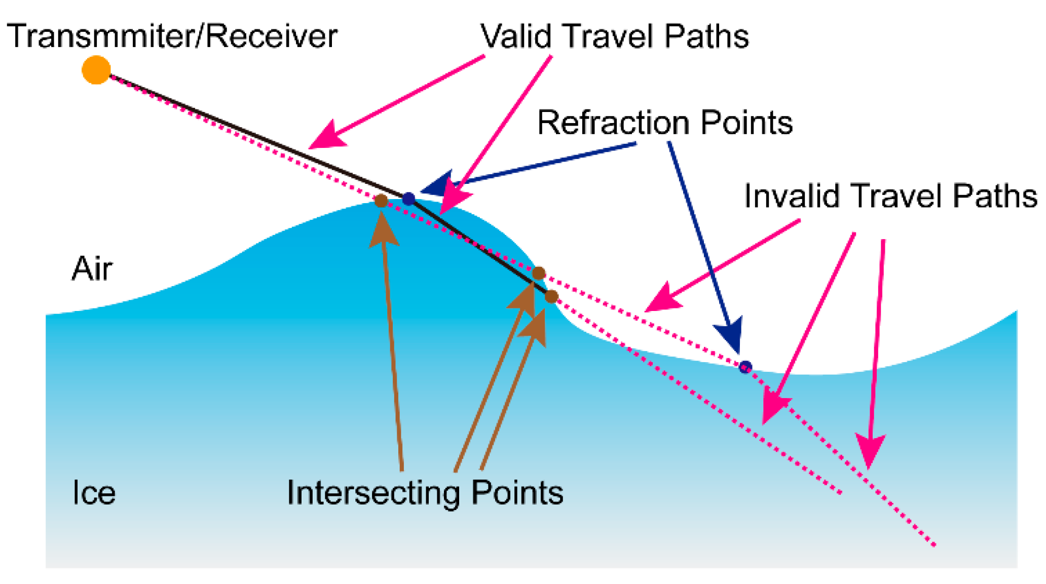
Figure 2.
Illustration of refraction.
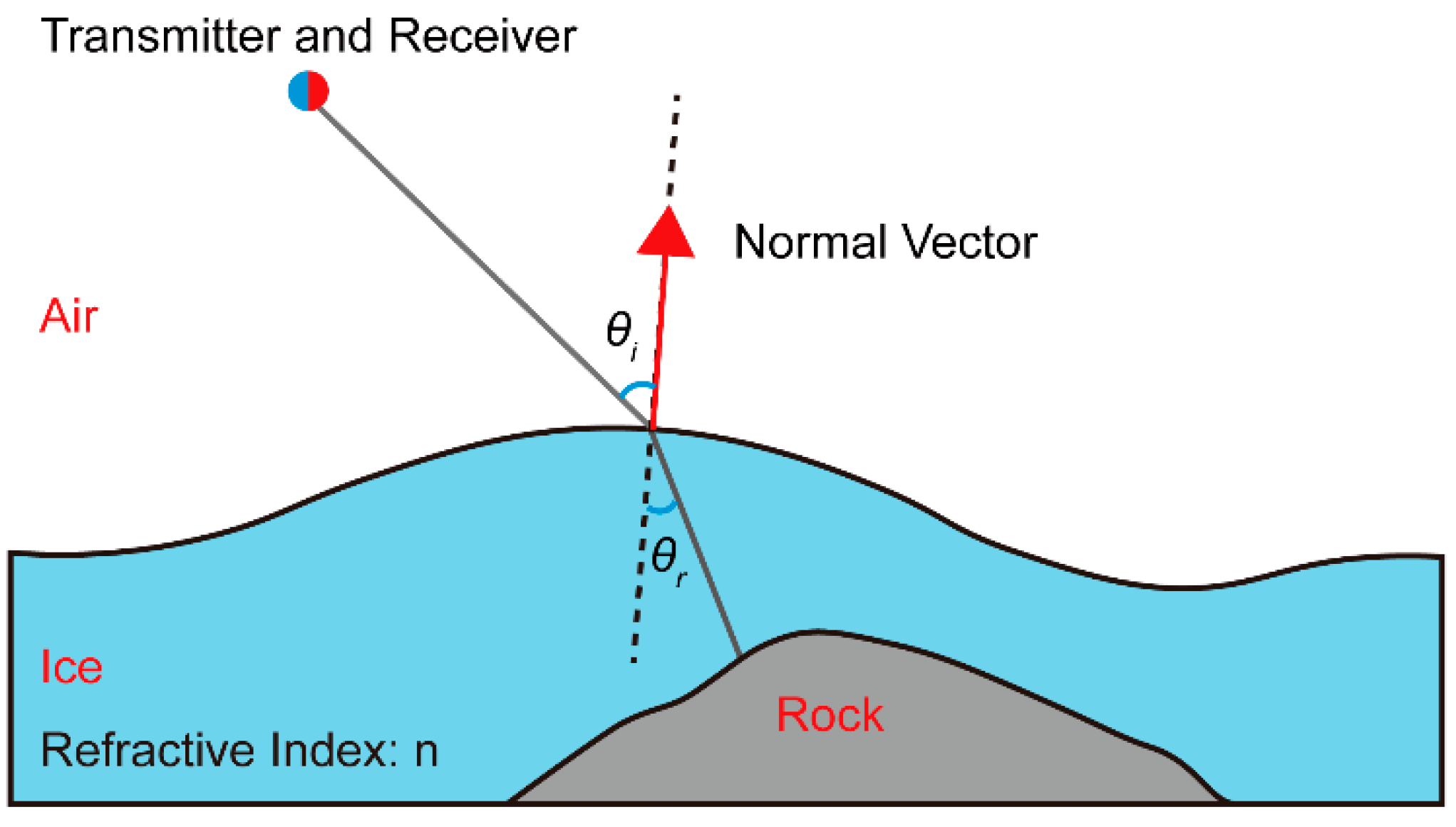
Figure 3.
Derivative of the Blackman-Harris window function in time domain and frequency domain. (a) current signal, (b) and (c) current signal amplitude and phase, respectively.
Figure 3.
Derivative of the Blackman-Harris window function in time domain and frequency domain. (a) current signal, (b) and (c) current signal amplitude and phase, respectively.
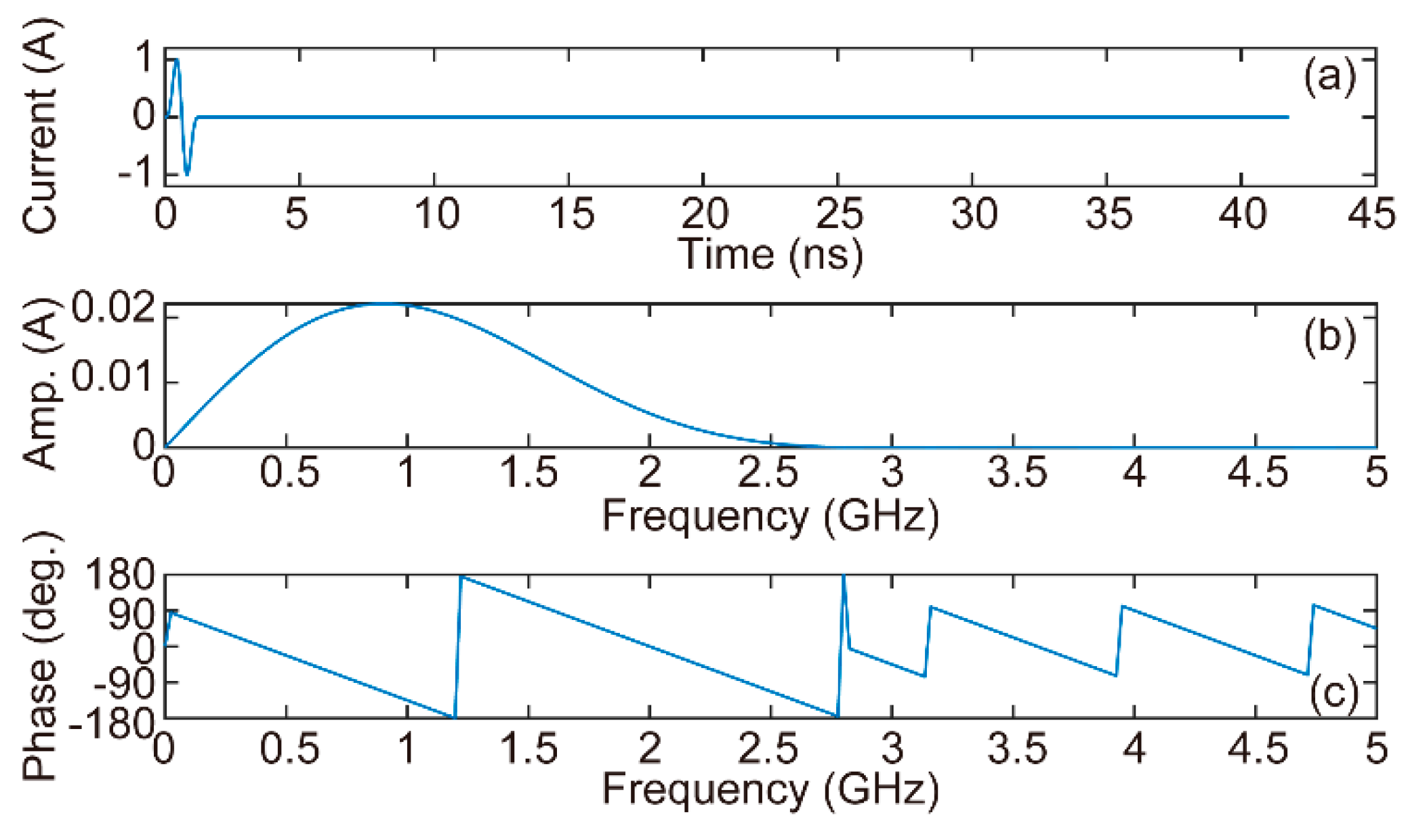
Figure 4.
The test of Model-2D-HAI-SIG. (a) Model-2D-HAI-SIG model; (b) FWD results of AGPR survey for the Model-2D-HAI-SIG model; (c) and (d) imaging results obtained using the CRTM and PBP algorithms, respectively.
Figure 4.
The test of Model-2D-HAI-SIG. (a) Model-2D-HAI-SIG model; (b) FWD results of AGPR survey for the Model-2D-HAI-SIG model; (c) and (d) imaging results obtained using the CRTM and PBP algorithms, respectively.
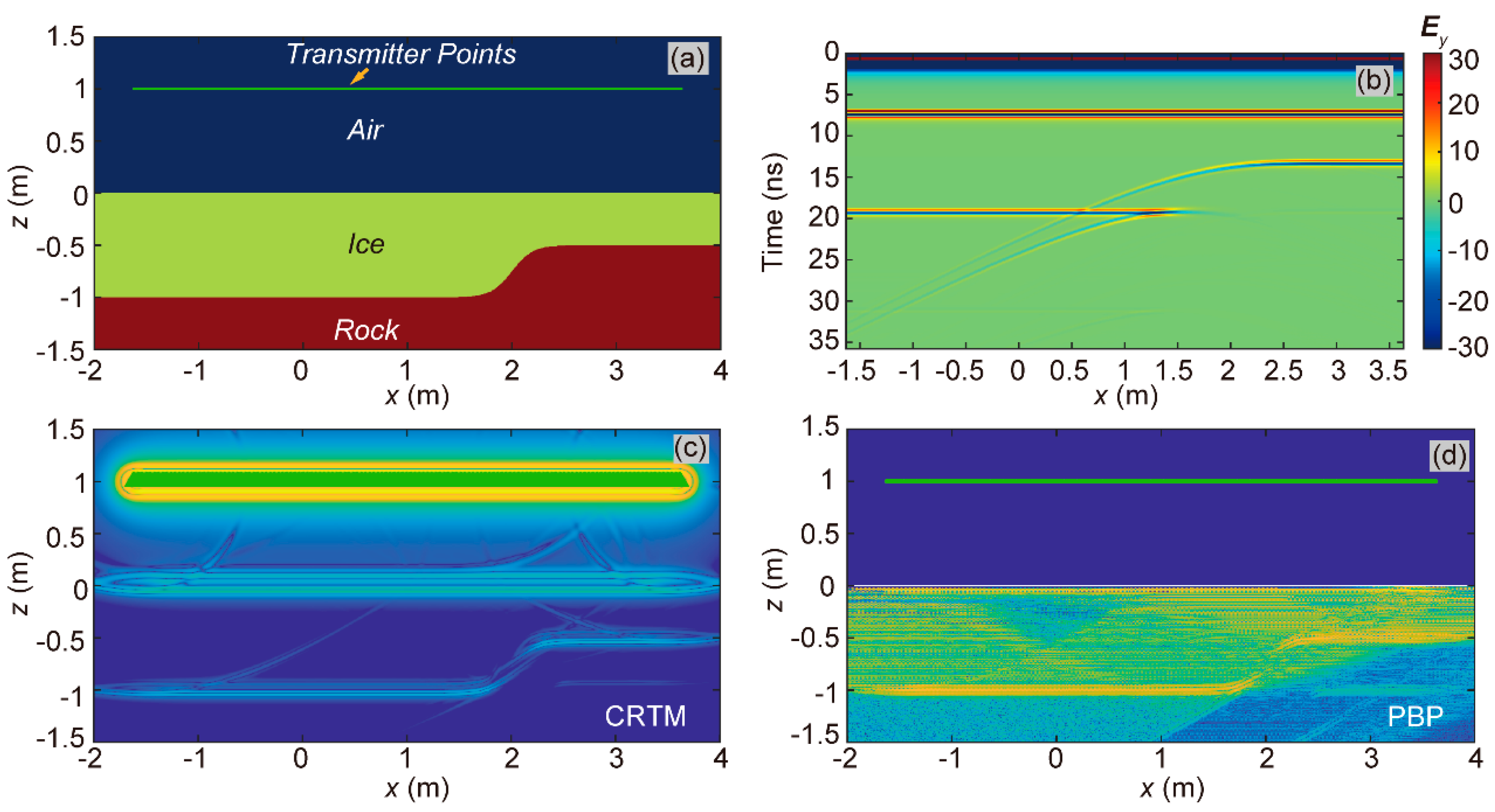
Figure 5.
The test of Model-2D-SAI-HIG. (a) Model-2D-SAI-HIG model; (b) FWD results of AGPR survey for the Model-2D-SAI-HIG model; (c) and (d) imaging results obtained using the CRTM and PBP algorithms, respectively.
Figure 5.
The test of Model-2D-SAI-HIG. (a) Model-2D-SAI-HIG model; (b) FWD results of AGPR survey for the Model-2D-SAI-HIG model; (c) and (d) imaging results obtained using the CRTM and PBP algorithms, respectively.
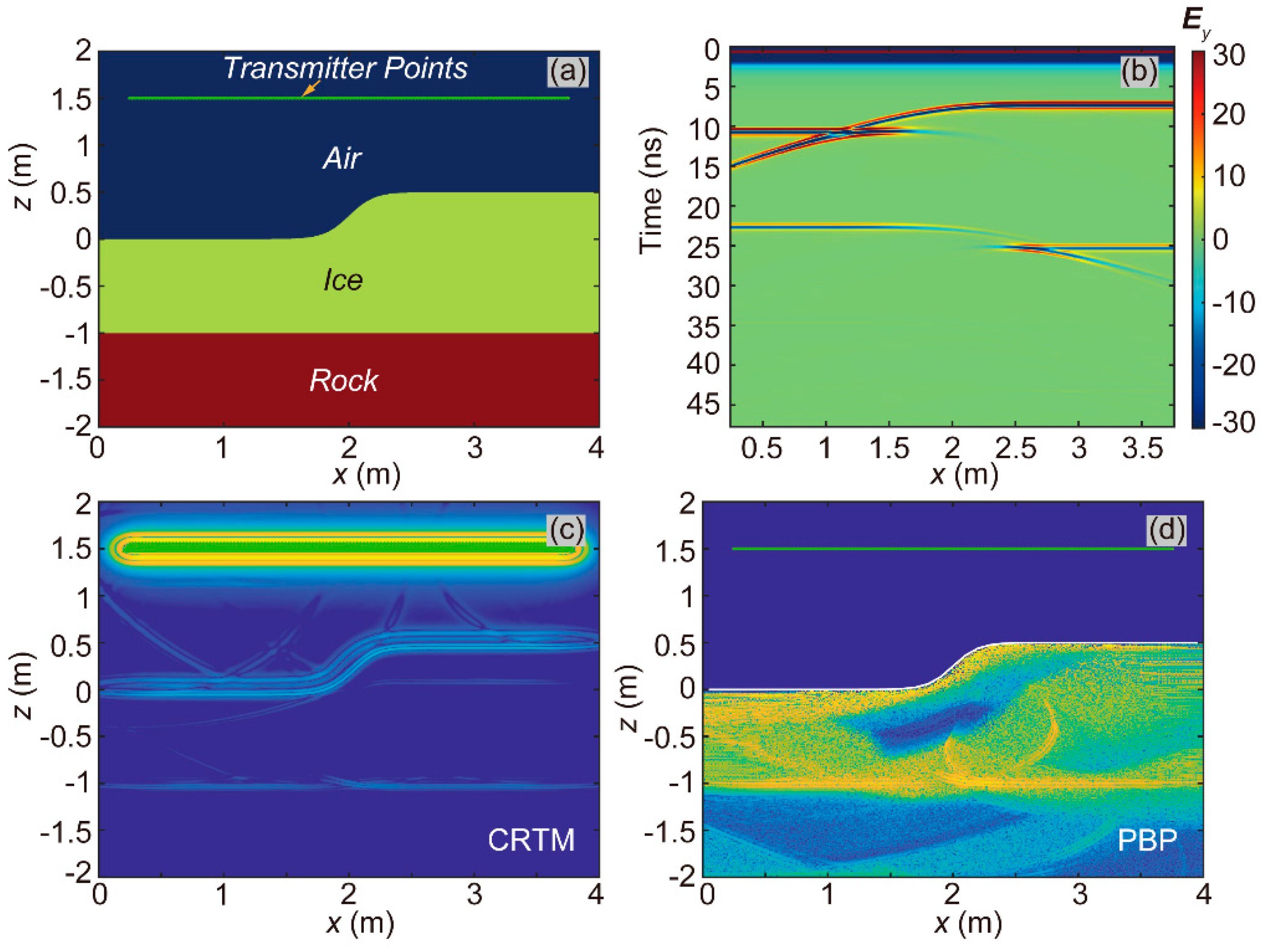
Figure 6.
Model-2D-SAI-SIG test. (a) model geometry (transmitter array on the green line); (b) AGPR forward modeling results; (c) and (d) results of the CRTM and PBP algorithms, respectively.
Figure 6.
Model-2D-SAI-SIG test. (a) model geometry (transmitter array on the green line); (b) AGPR forward modeling results; (c) and (d) results of the CRTM and PBP algorithms, respectively.
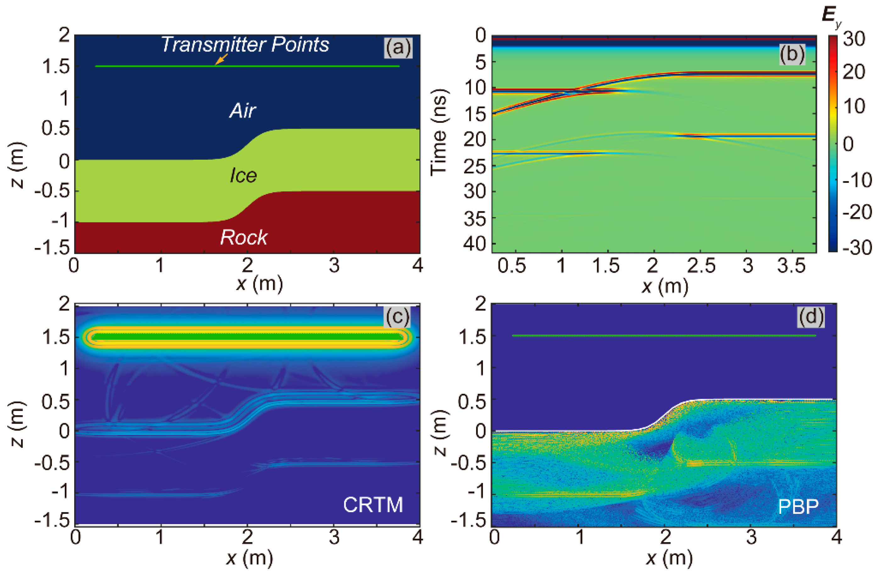
Figure 7.
The test of Model-2D-HAI-HIG-F. (a) Model-2D-HAI-HIG-F model; (b) FWD results of AGPR survey for the Model-2D-HAI-HIG-F model; (c) and (d) imaging results obtained using the CRTM and PBP algorithms, respectively. The horizontal fracture was named F1; the tilted fracture was named F2; and the vertical fracture was named F3.
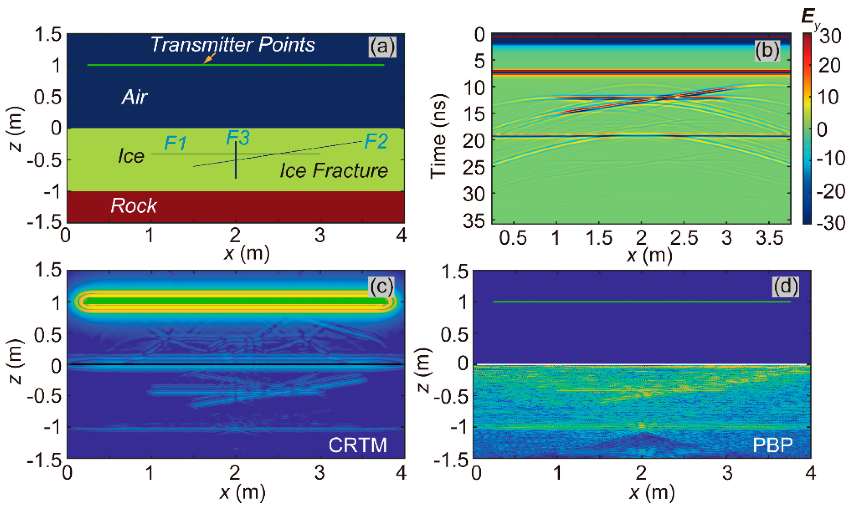
Figure 8.
Model-3D-HAI-SIG test. (a) model geometry (transmitters are indicated by the blue dots); (b) AGPR forward modeling results; (c) and (d) results of the CRTM and PBP algorithms, respectively.
Figure 8.
Model-3D-HAI-SIG test. (a) model geometry (transmitters are indicated by the blue dots); (b) AGPR forward modeling results; (c) and (d) results of the CRTM and PBP algorithms, respectively.
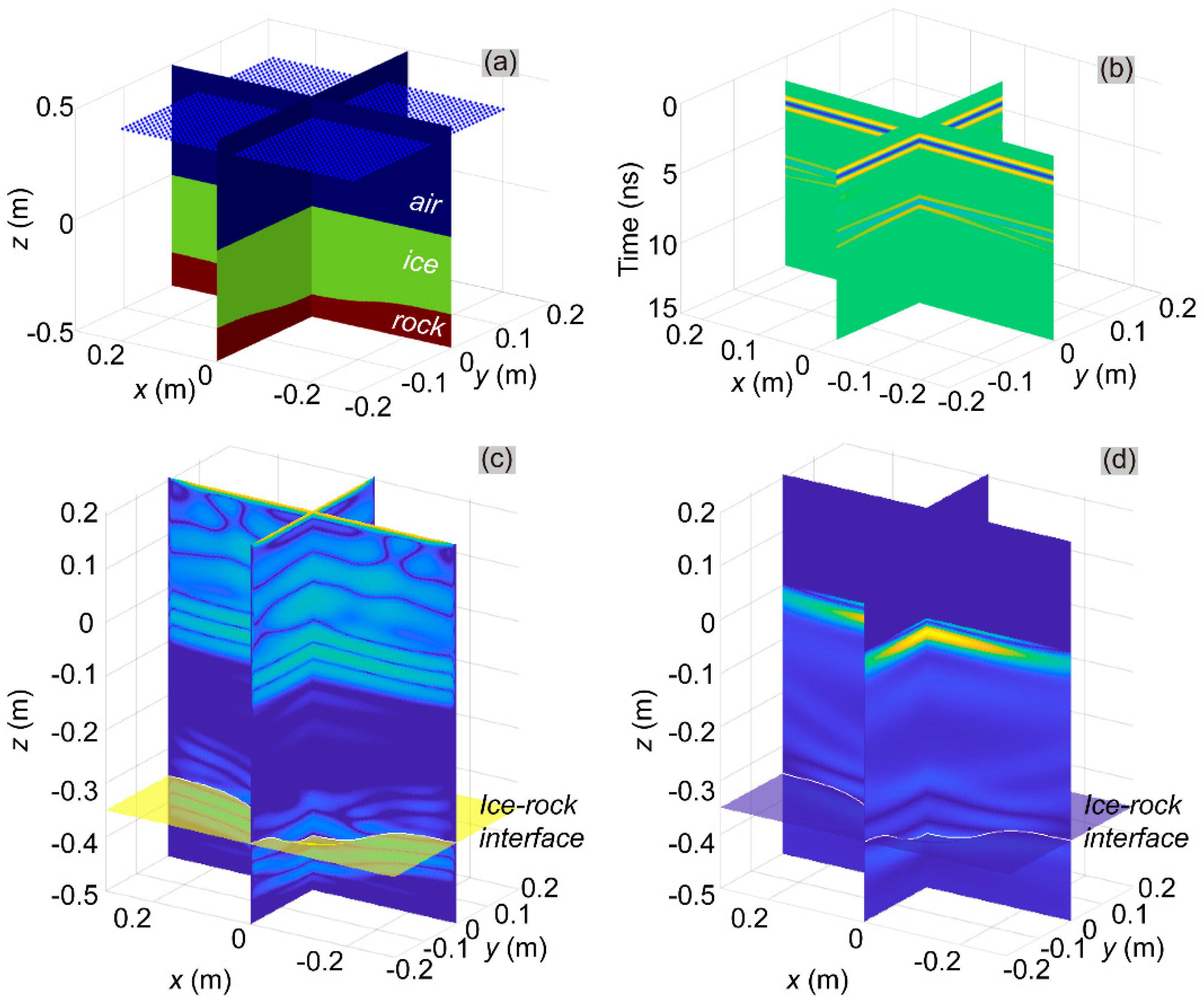
Figure 9.
Schematic diagram of the geometric strategy for identifying strong backscattering nodes at the subglacial interface. TR represented the transmitting/receiving antenna; gai denoted arbitrary discrete grid nodes on the air-ice interface; vai represented the normal vector of the air-ice interface at point gai; ptr-ai denoted the vector pointing from gai to TR; vig represented the normal vector of the ice-ground interface at point gig; pai-ig denoted the vector pointing from gai to gig; θerr denoted the angle between the vectors of (-pai-ig) and vig.
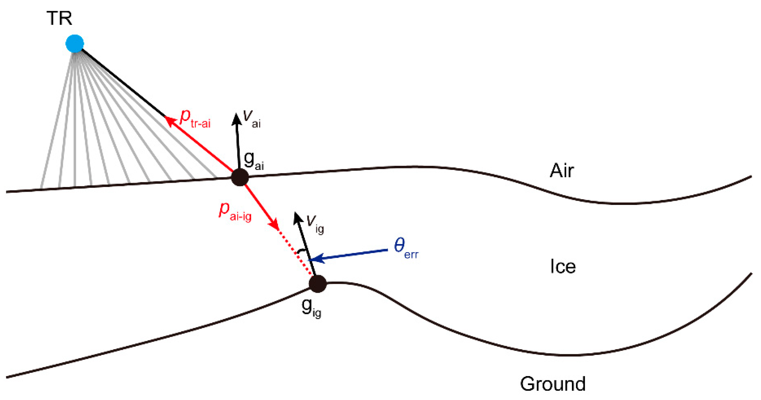
Figure 10.
Analysis of strong backscattering mechanisms. (a) triangles indicate the analytically predicted locations along the ice-rock interface in Model-2D-HAI-SIG that satisfy the geometric conditions for strong backscattering; (b) triangles mark the corresponding time positions in the radar profile (B-SCAN) that were theoretically predicted to exhibit strong backscattering signals, matching the interface locations shown in (a); black triangles in (b) correspond to the white triangles inside the black box in (a); blue triangles in (b) correspond to the white triangles inside the blue box in (a).
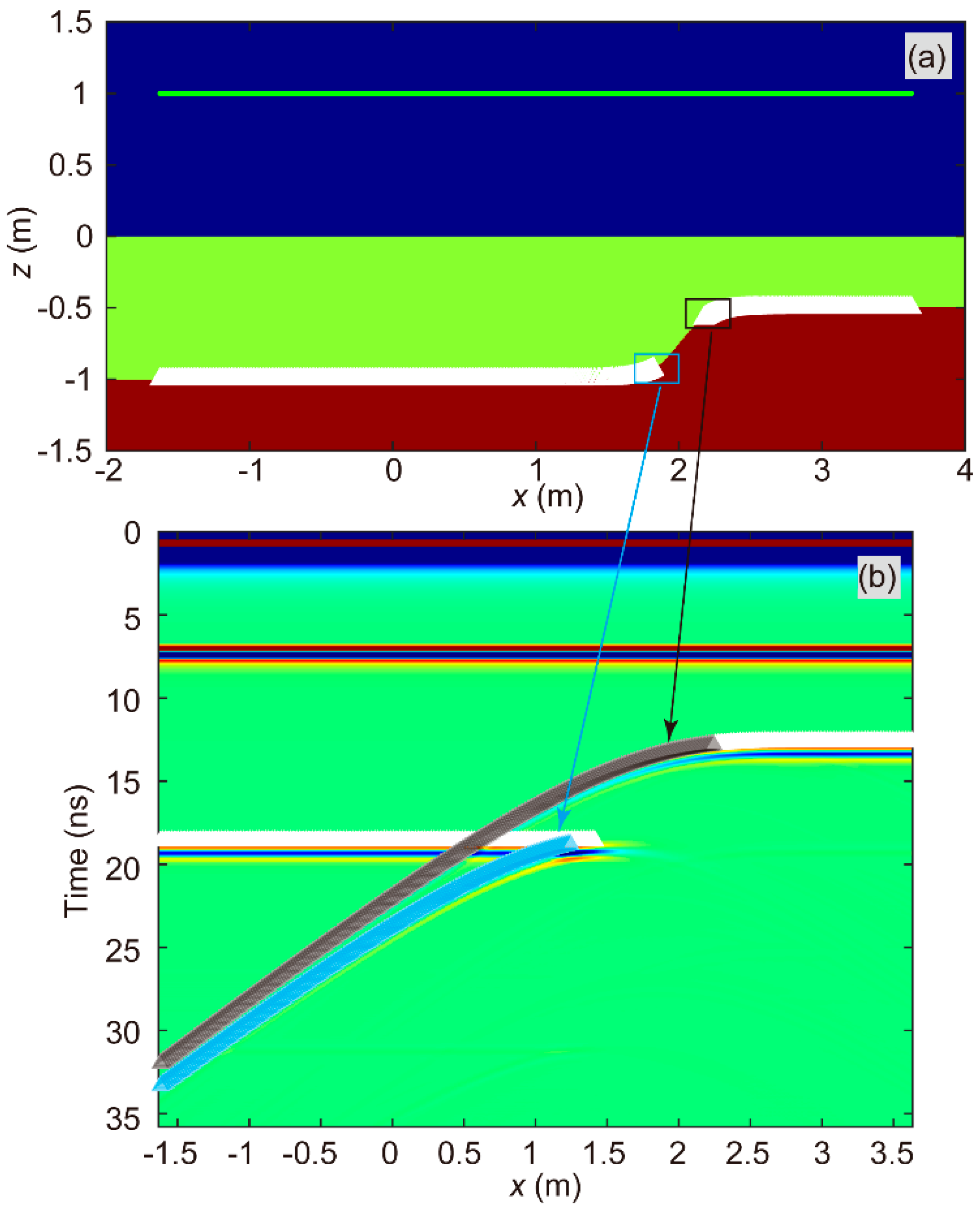
Figure 11.
Assessment of Backscattering Effectiveness and Spatial Distribution Characteristics at the Ice-Rock Interface. Segments of the ice-ground interface that could not generate strong backscattered signals were colored red.
Figure 11.
Assessment of Backscattering Effectiveness and Spatial Distribution Characteristics at the Ice-Rock Interface. Segments of the ice-ground interface that could not generate strong backscattered signals were colored red.
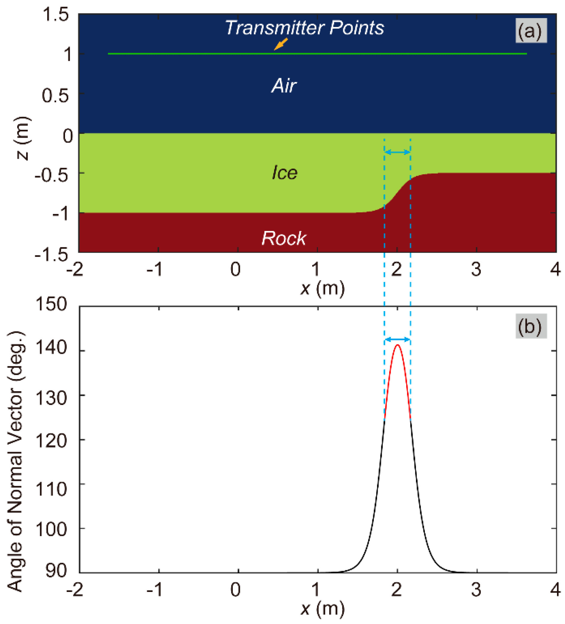
Figure 12.
Time-domain slices from the forward modeling computations of Model-2D-HAI-SIG, with transmitters arrayed on the steeply inclined interface. (a) 701st time step; (b) 1001st time step; (c) 1401st time step; (d) 2201st time step; (e) 2901st time step; (f) 4001st time step, where green triangles indicate radar transmitter positions.
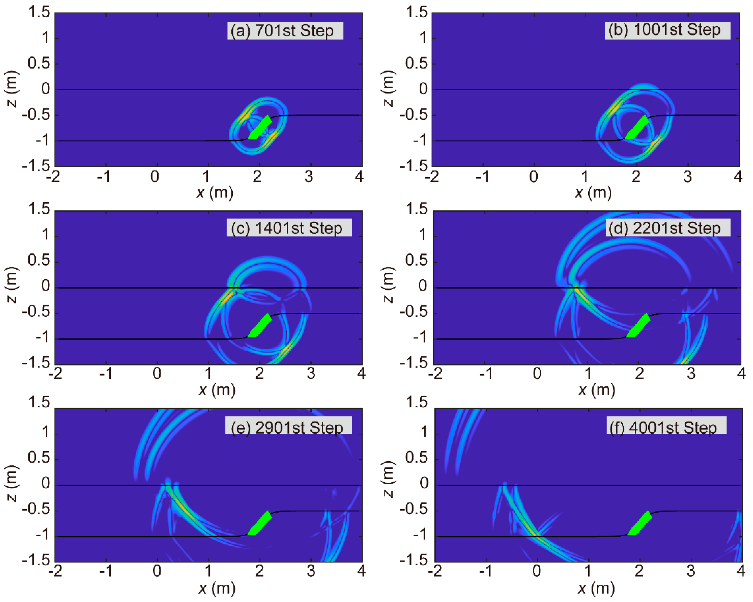

Table 1.
The electromagnetic properties of air, ice, and rock used in this study.
| Matter | Relative permittivityε | Relative permeability μ | Electric conductivity σe (siemens/m) | Magnetic conductivity σm (ohms/m) |
| Air | 1 | 1 | 10-10 | 0 |
| Ice | 3.2 | 1 | 10-5 | 0 |
| Rock | 5 | 1 | 10-3 | 0 |
Disclaimer/Publisher’s Note: The statements, opinions and data contained in all publications are solely those of the individual author(s) and contributor(s) and not of MDPI and/or the editor(s). MDPI and/or the editor(s) disclaim responsibility for any injury to people or property resulting from any ideas, methods, instructions or products referred to in the content. |
© 2025 by the authors. Licensee MDPI, Basel, Switzerland. This article is an open access article distributed under the terms and conditions of the Creative Commons Attribution (CC BY) license (http://creativecommons.org/licenses/by/4.0/).
Copyright: This open access article is published under a Creative Commons CC BY 4.0 license, which permit the free download, distribution, and reuse, provided that the author and preprint are cited in any reuse.


