
Submitted:
31 August 2025
Posted:
02 September 2025
You are already at the latest version
Abstract
Background: In general, this methodical paper describes a well-documented application of one complexity measure and various machine learning methods to solve a specific problem in biosignal processing: predictions of ventricular tachycardia & fibrillation and Torsades de Pointes arrhythmia. The methodology part provides a concise introduction to all used methods and is accompanied by a sufficient citation apparatus. Once the presented methodology gets explained, it is easy to apply it to many other research areas. Currently, allopathic medicine is facing one of the biggest challenges and transitions that it has been going through during its history. Deeper understanding of human physiology will enable medicine to reach better understanding of human body functioning. Simultaneously it will allow to design novel, so-far-inaccessible, complex, dynamically changing therapies based on this knowledge. We address the following general question: "Are there existing mathematical tools enabling us to predict changes in physiological functions of human bodies at least minutes or even hours before they start to operate?" This general question is studied on a specific, simple model of the rabbit heart subjected to by medically-induced drug insults that are leading to the drug-induced Torsades de Pointes (TdP) arrhythmia. This class of models can improve our ability to assess the current condition of the heart and even to predict its future condition and disease development within the next minutes and even hours. This can eventually lead to substantial improvement of the out-of-bed cardiology care. Methods: Electrocardiograph (ECG) recordings were acquired—in a different research project—from anesthetized rabbits (ketamine and xylazine) that were subjected to infusion of gradually increasing doses of arrhythmia-inducing methoxamine and dofetilide drugs. Subsequently, ECG curves were evaluated using the permutation entropy for different lag values, where the lag is the evaluation parameter. Lag is defining the distance between neighboring measuring points. Computed entropy curves were processed by machine learning (ML) techniques: Random Forest (RF), Support Vector Machine (SVM), Logistic Regression (LR), k-nearest neighbors (k-NN), Ensemble Learning (EL), and others. ML methods performed classification of arrhythmia above the evaluated segments of permutation entropy curves. Results: A possibility to predict drug-induced TdP arrhythmia up to one hour before its onset was confirmed in a small study of 37 rabbits with specificity and sensitivity achieving 93% (for important statistical features [measurable properties]). It was demonstrated that animals can be divided into two distinct groups: susceptible and resistant to arrhythmia. It was shown that animals can be classified using just five-minute segments prior to and after the application of methoxamine (this drug can be used in human medicine, unlike dofetilide). The drawback of the study is the too low a number of measured animals. Conclusion: This pilot study demonstrated a relatively high probability that the prediction of the onset of TdP arrhythmia is possible tens of minutes or even hours before its actual onset with sensitivity and specificity around 93%. Those findings must be confirmed in wider animal studies and on human ECGs. Another human study got similar results using deep learning methods. Presented software predicting of arrhythmia has a big potential in human medicine, because it can be applied in hospital monitors, implantable defibrillators, and wearable electronics guarding the health condition of patients. A small set of tested animals does not allow their subdivision into sufficiently big subgroups (TdP and Normal). Groups are too small and asymmetric. It is recommended to test achieved results on different, larger ECG databases of animal models and on large human ECG databases.
Keywords:
arrhythmias
; Torsades de Pointes
; ECG
; complex systems
; entropy
; permutation entropy
; prediction
; machine learning
; rabbit model
; methoxamine
; dofetilide
1. Introduction
Medicine is facing one of the biggest challenges it has gone through during its history. It is gathering ever-increasing amount of imaging, genetics, epigenetics, proteomics, interactions of cells with drugs, raw physiological, and other types of data. Despite such a huge amount of information—it is better to say, due to it—in most cases, we are unable to understand the functioning of body parts and systems, including the physiology of human bodies, to the level applicable in therapy. We are aware of the fact that a deep understanding of regulatory mechanisms existing and operating at the levels of cells, tissues, organs, and bodies is critical for understanding many diseases, their causes, and their possible therapies. Fortunately, some of those hidden regulatory mechanisms just started to be revealed. This brings us to the main goal of this paper.
We are aware of the fact that deeper understanding of different segments of human physiology will enable medicine to make a crucial step towards better understanding of human body functioning as a whole and to design novel, so-far-inaccessible, complex, dynamically changing therapies based on this knowledge. Hence, we address the following general question:
This general question will be studied on a specific, simple model of the rabbit heart that is leading to the drug-induced Torsades de Pointes (TdP) arrhythmia [1,2,3,4,5,6,7].
Currently, we are already aware of the fact that organs and their regulatory systems are mutually influencing each other, but we are still mostly unable to reveal the exact topology, interdependence, and real effects of those regulatory networks and to quantify them (e.g., see books on the application of AI in medicine [8,9], examples of the central nervous system and emotions [10,11], and the heart [7,12]). To achieve this goal, the following steps must be accomplished: (a) huge data sets of digitized, physiological recordings must be collected (e.g., ECGs, EEGs, breath patterns) with their relevant medical classification (distinction among various cases), (b) they must be provided as open access data (with citations of teams which are providing them plus their responsibility), (c) data will serve as the calibration tool to all newly developed mathematical methods and as means of comparison of various methods (there will be available versions of databases and their closing dates), (d) all newly developed mathematical tools and methods will be tested on them, (e) physiological dependencies will be gradually revealed and cross-tested, (f) only tested therapies based on such physiological knowledge will be used medically, (g) any failure of an already developed method will be studied and initiate the improvement of the database, and (h) medicine can gradually achieve holistic modularity (this means that it can be treated locally while being aware of holistic responses due to knowledge of physiology networks) in this way. This automatically leads to a possibility of highly individualized therapies and not statistically based therapies (RCTs). There already exists a whole range of successful pilot physiological studies in some areas, providing proof of the vitality and importance of this approach [13,14,15,16,17,18,19,20,21,22,23]. Unfortunately, researchers are still quite far from mapping the whole physiology in this way; one of the reasons is a lack of knowledge about emergent information processing that relies on the massively-parallel nature of all living systems [24,25,26,27].
The current physiological research on animals and humans faces several principal difficulties and obstacles, which inevitably occur during any attempt to better describe, understand, and predict the actual physiological state of the various bodily functions. The first obstacle: an intricate network of physiological processes (further called the physiological network) where said processes are often mutually entangled in unexpected ways across all organ systems just started to be revealed. The second obstacle is that when a particular physiological process is studied, we do have to be aware of those interconnections through the physiological network, as it can easily modulate and change the behavior of the studied part according to the changes within the rest of the network (e.g., the heart is heavily influenced by adrenal and thyroid hormones or by the autonomous nervous system). There does not exist an ideal stable operational mode/fixed point within the physiological network operation. Contrary to it, we know that physiological network is constantly changing and adjusting according various physiological inputs (physical or mental stress, digestion, relaxation, etc.).
That all together is a quite challenging situation from the mathematical perspective. It can be said that the structure of the physiological network possess a unique position within the context of the modern medicine and one of the biggest, if not the biggest, challenges in better understanding living organisms in health and disease. Once this network is understood, it will enable medicine to handle diseases and deal with various physiological disturbances from a completely new position using so far unknown and inaccessible treatments. Development of such novel methods and tools enables medicine to measure, to understand, and finally to change and control physiological states of bodies with unprecedented precision.
There are existing many approaches that are enabling measurement of the complexity observed in biomedical systems, for example, entropy [28,29,30] (with its novel reinterpretation [31,32] linking it with information), fractals [33], or statistical [34] measures. The main idea behind the construction of various measures of complex systems (CSs) is our inability to trace all subtle details of evolving CSs [35]. Instead, we map the whole system into its simplified form using some kind of measure (see below for an example and detailed description). In the following, we focus our attention to information entropy measures [30,36,37]. A set of the key mathematical tools—which importance has been recently recognized and with one of them used in this study—that are enabling to measure and quantify CSs properties is composed of various types of information entropy: ApproxEn [13,38,39], SampEn [13], PeE [40], multiscale entropy [15,41,42], and others [19,28,43,44].
Entropy is typically designed in such a way that it maps the whole system into a small, restricted set of K bins with probabilities . Bins are giving the information about the frequency of an observed event/value falls in a given bin . Those probabilities are inserted into the entropy equation. The generic entropy equation [45,46], is measuring variability of probabilities across all those bins and hence, indirectly, measuring the observed system. All systems that are giving a constant output, i.e., the only one bin is nonzero with for one index j, have entropy equal to because for . Whereas, the white noise (all bins have the same probabilities for all ) has the highest possible value of entropy because, in such a case, all states of the system are visited equally; the value of increases with the value K. All probabilities equal to zero are omitted from the sum (otherwise they will contribute by infinity values in the entropy equation; that is an unwanted situation).
As already mentioned, better understanding of CSs achieved during the past 20 or 30 years yielded an increasing number of specialized CS measures that are capable of observing major and even subtle changes in biosignal recordings, which are otherwise not accessible to even highly trained specialists, even when using very precise biosignal recordings. The explanation of the major obstacle in the humans comprehension of those biosignals follows. Humans are unable to precisely follow, measure, and classify long intervals of signals having lengths of tens of seconds or even minutes simultaneously. This task must be accomplished for many biosignals simultaneously. That is beyond human comprehension and capabilities, but it is ideal for computer algorithms.
This is the moment when AI and machine learning techniques step in and provide us tools to distill information and classify various behaviors and modes of CSs with unprecedented precision [8,9,47,48,49,50,51]. The exact procedure of applying ML methods is explained and studied in depth in this case study, which is dealing with physiological changes in heart functioning. The input for this paper is an animal study on rabbits [52], which were subjected to extremely harsh conditions generating arrhythmias that were artificially induced by the application of arrhythmogenic drugs (anesthetics and cardiomyocyte ion-pump disruptors). The heart occupies a unique position within all physiological studies [7,12] because it can be easily, indirectly observed using ECG recordings (we use ’ECGs’ and ’ECG recordings’ interchangeably in the following text) due to the heart’s very strong electromagnetic fields. Similarly, brain observation by EEGs provides another rich source of physiological data [16,17]. Unfortunately, other organs do not provide us with such precious physiological data sources due to our inability to detect and measure them as easily and precisely as is done for hearts and brains.
This brings us to the core of this paper: the prediction of drug-induced arrhythmias, which originate in the dispersion of the action potential propagation velocities across the thickness of the ventricular walls. This could lead, under certain conditions, to the creation of a reentry system leading to focally unstable ventricular arrhythmias that are meandering through ventricles, and that are called Torsades de Pointes (TdP) arrhythmia [3,4,5,6]. The spiral tip meandering within ventricles—and hence, the location of the reentry system—leads to the typically observed periodic changes of the modulation of the ECG channel amplitudes during TdP arrhythmia because the projection of action potentials into the fixed electrodes is changing with the changing position of the spiral tip. A part of TdP arrhythmia ends spontaneously, but a non-negligible number of them lead to a ventricular fibrillation or flutter and subsequently to a cardiac arrest followed by a death within minutes. Due to TdP’s unpredictability in some patients—even after ruling out long QT syndrome patients who are highly susceptible to TdPs, [1,2,3,44] and those with a genetic predisposition—TdPs are called, for a good reason, a silent killer.
Only a smaller portion of TdPs is observed within in-patient settings. The actual number of heart arrests caused by TdPs is unknown because it cannot be decided by an autopsy. There exists a still-growing list of drugs that can cause the onset of TdPs in predisposed patients. Often, it comes as a complete surprise to many people that the main cause of drug-induced TdPs results from the use of drugs that are not primarily used to treat heart diseases (e.g., anti-arrhythmics, etc.) [1,2,3] but they somehow manage to disrupt or to interfere with ion channels of cardiomyocytes (including some drugs treating mental disorders by modulation of ion channels in neurons, PPIs, immunosuppressive drugs, etc.). This poses a relatively large risk for patients that have never acquired any heart disease or disturbances during their lives because the occurrence of TdPs is not expected in them (unfortunately, the fraction of unknown susceptible patients is unknown). The ideal solution requires an in-hospital cardiology observation of all patients—or at least several ECG checkups—during the initial stages of the application of those potentially TdP-generating drugs, which is based on acquiring an ECG on a regular basis and searching for their undesired changes.
For example, during the period of time from February to April 2020, when COVID-19 had been spreading in the world, there were existing large cohorts of well-followed patients who were experiencing TdP arrhythmia. The reason was that some of the latest therapies for SARS-CoV-2 are using hydroxychloroquine and azithromycin, chloroquine, and combinations with other antiviral drugs, leading in a high proportion of cases to long QT syndrome and a great risk of TdP arrhythmia—it can be up to 11%, according to this study [3]. Well documented recordings of those patients can serve as inputs to a database that can be utilized in development of ML methods predicting TdP arrhythmia.
For those reasons, techniques observing prolongation of the QT interval were developed: prolongation of the QT interval is caused by an increase in the variation of action potential duration in different parts of the heart wall. A prolongation of the heart rate corrected interval above 500 ms is a marker of patients that have a high probability of developing TdPs [4,5,6]. Recently, genetic studies enabled narrowing of the pool of all TdP-susceptible patients by the use of genetic markers. Despite a great effort, there are still many patients who develop a TdP, which is not detectedable by the previous criteria, in out-of-hospital settings—this puts those patients in danger.
It is the exact moment when complex systems can take their place with the already well-established notion of information entropy [36,37]. In the recent two or three decades, many information entropy measures have been developed across many disciplines [16,17,53]. Simply said, the actual value of an information entropy measure at a given moment enables to assess the operational state/mode of the underlying CS. Many types of entropy measures demonstrated their usefulness in the processing of biosignals originating in different parts of the physiological network [20,42,54,55]. ECG signals contain a vast amount of hidden information that just started to be understood and become decodable, which represents a great potential for future research. Permutation entropy () can reveal hidden information with high precision [56,57,58]. It is achieved using relatively short signals when compared to other techniques, as is, e.g., heart rate variability (HRV) [59,60,61,62]. Processing ECGs using provides a greater deal of the underlying information, which is impossible to reveal by any standard analytic or statistical method. Due to the complicated nature and high dispersion of information among entropy data, it is necessary to apply ML techniques that are capable of revealing those hidden dependencies [8,9,47,49,51,63].
The main goal of this work is to demonstrate that a proper use of the carefully selected CSs measures with the support of ML techniques can reveal unprecedented details from the physiological network. This study is a pilot study of a whole set of possible, more detailed studies that can, one by one, pinpoint so far inaccessible information flows and predictive markers of physiological changes within the physiological network. In the case of drug-induced TdP arrhythmia, it is demonstrated that arrhythmia prediction can be performed with a relatively high precision even on a small set of ECG recordings.
The availability of wearable devices is increasing in sync with their increased penetration within the society. Once the reliable algorithms predicting various life-threatening heart diseases including this algorithm, become available with the specificity and sensitivity high enough, they can be applied in wearable devices and literally save a lot of lives. Due to public safety, the first mandatory applications of such types of algorithms—and devices based on them—will be very probably used in occupations like driver, pilot, astronaut, industrial operator, etc. where a lot of lives and property is at stake due to a potential health collapse of the operator. It can happen due to a heart attack, arrhythmia, ongoing stress, or distress. Currently, detection devices are mostly developed and tested in cars [64,65]. Detection of stress and psychological state of the drivers/pilots can help avoid accidents and catastrophes [66,67].
This paper deals with the problem of solving the long-term prediction of physiological changes of the heart, which was studied on a pilot, rabbit model where two different cardiomyocyte ion channels modulating drugs were delivered (methoxamine and dofetilide) along with anesthetics (ketamine and xylazine) to studied animals. Some of those rabbits were susceptible to double- and triple-chained premature ventricular contractions (PVCs). Double- and triple-chained PVCs were, in a fraction of the cases, developing into Torsades de Pointes arrhythmias, and those were typically lasting between one and two hours during experimental observations. Firstly, and most importantly, the whole study serves as a template of research strategies that can be applied in similar cases from the complex systems and ML methods points of view. Secondly, the study paves the way towards a completely new class of predictive tools working in real time that are capable of performing a reliable, long-term prediction of physiological functions.
Why is this methodical paper designed in this way? It is written from three distinct points of view: complex systems, biology & medicine, and computational mathematics. Readers coming from different areas of research might find some paper parts redundant due to their expertise. Basically, this paper should be readable to all groups of readers. Nevertheless, it is still the publication about mathematical and computational methods used to classify biological signals, but it is mathematically demanding (introductory and method sections should enable every reader to fill the gaps in the theory).
The structure of the paper is as follows: the role of AI and machine learning in biomedical research in Section 2, a brief introduction to information entropy in Section 3, results of (TdP + non-TdP) vs. non-arrhythmogenic rabbits in Section 4, narrowed results of TdP vs. non-arrhythmogenic rabbits in Appendix C, discussion in Section 5, data & methods in Section 6, and Appendixes A.1-A.3.
2. Importance and Role of AI and Machine Learning Techniques in Biomedical Research
Over many millennia, science has been gradually developing a set of increasingly sophisticated mathematical approaches, methods, and theories enabling us to quantify, describe, and predict observed natural phenomena. Currently, as everyone knows, we do have geometry, arithmetic, algebra, calculus, statistics and probability, differential equations, chaos, fractals, mathematical & computational modeling, and simulations within our mathematical toolkit. We are continuously developing even more advanced tools; see for details [63,68].
Historically, initially, humans were working with simple numbers used for counting possessions that were soon extended to arithmetic. Simultaneously, the necessity to administer large land areas led to the development of geometry. There had been a long period of stagnation after which infinitesimal values, limits, and calculus with differential equations occurred during the 17th century. This enabled researchers to study physical bodies and develop advanced mechanical theories (e.g., celestial mechanics). Those were later, in the 20th century, extended into deformation of bodies, heat diffusion, and fluid flows described by partial differential equations (implemented using finite element methods). During the 17th century, the development of statistical approaches in physics that are describing ’fluid bodies’ consisting of large ensembles of simple particles (gases, liquids) had started. Those parts have some fixed properties, averages, or distributions, that do not change with time; and hence, the systems under study can reach only some well-defined global states. Studies of large ensembles of atoms and molecules led to development of statistical physics in the 19th century and to the notion of entropy [69,70,71]. In the 20th century, we developed deterministic chaos [72], chaos [73,74], and fractal [75] theories that enlarged the mathematical toolkit with methods enabling us to describe more sophisticated natural phenomena (weather, solitons, phase transitions, and some emergent structures).
So far, all biomedical theories and models had been based on the application of functions, equations, and more or less defined dependencies, or on statistics & probability [76]. From the current state of the biological and medical research, it is seen that models based on the above-provided mathematical frameworks fail to describe most of the phenomena observed in those complicated biosystems. What are the main causes of this failure? Currently, scientists are aware of the fact that mean field approximations, which are applied in deriving dependencies among variables, differential equations, and statistical parameters of biological phenomena, are insufficient in capturing and reproducing the fundamental processes operating within biosystems. Let us take a closer look at it.
What are omitted and not well described fundamental processes critical for the precise evaluation and prediction of biological systems’ behavior? Those are mutual interactions among a system’s constituting parts that are operating within the given biological system under consideration, e.g., the human body. Proteins, signaling molecules, genes, epigenetics, distinct regulatory mechanisms, cells, organs, and tissues with their well-defined one-to-one, one-to-many, and many-to-one interactions, which are often spanning multiscale levels, are the key.
Scientists arrived and started intensively studying a theoretical and modeling concept, which can be applied to such a class of problems, that has been developing since around 1980. Simply put, researchers realized that there exists a huge number of systems that are based on interactions of large numbers of relatively simple components that are mutually interacting in parallel within some restricted neighborhood of each component. From and through those interactions, global properties of the system raise, including self-organization, emergence, self-assembly, self-replication, and a whole range of similar phenomena. Gradually, researchers arrived at the concept of complex systems that is often called complexity (do not confuse with complexity of algorithms from the theory of computing); see for the review [63,68]. It is a known that complex systems, when well-defined from the beginning—it is meant their local spatio-temporal interactions—produce surprisingly robust and generic responses that are easy to be identified with observed natural phenomena.
Natural phenomena observed in biology and medicine are not efficiently describable by any of the above-mentioned mathematical approaches except the last and newest one. This leads us naturally to the latest mathematical description, briefly described above—which started to be increasingly applied in biology and medicine—to complex systems. Complex systems (CSs) enable us for the first time in the history of science to describe biological systems at the level of their systemic parts and their mutual interactions (see review of such complexity models [63,68] and research [24,25,27,77] along with citations there), as shown above.
The problem with the majority of complex systems-based models of biological phenomena is that their constituent elements are not known. Hence, researchers are incapable of building those models in ways that can be directly compared to observed phenomena. This obstacle in description and understanding of those biological phenomena can be overcome by application of artificial intelligence (AI), machine learning (ML), and deep learning (DL) techniques. Modern techniques developed within AI, ML, and DL [8,9,47,48,49,50,51,78] (see biomedical AI books [8,9]) enable us to distill dependencies—from the observed data produced by complex systems—that are otherwise invisible to all other before-mentioned approaches developed in mathematics. Generally, AI enables us to reveal dependencies that must be reproduced by all future, now non-existent, models of biological phenomena. In other words, AI enables us to identify and reconstruct global responses and dependencies of the biological systems that are driving their evolution even without any knowledge of their internal causes. It is possible to distill empiric dependencies in this way. That is why a combination of a well-selected complex system measure (permutation entropy) and machine learning techniques had been applied in this study. This explains research in one sentence.
3. Entropy: Motivation, Three Definitions, and Applications
The historical development of the concept of entropy is quite complicated to follow for non-specialists because it involves several distinct streams of thought—accumulated during centuries—that occurred independently during the development of various scientific disciplines: thermodynamics, statistical physics, and theory of information. It requires deeper understanding of all those disciplines. Such diversity of entropy definitions led, leads, and will lead to much misunderstandings. To make things even more complicated, the concepts and the interpretations of entropy are often misunderstood and misinterpreted even by trained physicists themselves. Awareness about this confusion is increasing, and there are attempts to resolve this confusion [31,32,79]. Not many researchers from across all research fields are aware of this fact—as they expect that there exists just one, ultimate, compact definition of the entropy—when they read about it in any scientific text. But the term entropy is always context-dependent.
This expectation is incorrect. In science, there exist only a handful of more convoluted terms throughout all literature. Briefly, the main source of difficulties with understanding of entropy lays in re-discovering and novel re-defining the notion of entropy within three distinct research areas and contexts: experimental physics (Clausius), theoretical physics (Boltzmann), and theory of communication and information (Shannon).
As explained above, this all created a great, persistent, long-lasting confusion among scientists coming from different disciplines in spite the fact that all definitions within their own research areas and their use there are mostly correct. In his era, Boltzmann himself was facing a big opposition when he proposed the kinetic theory of gases and explained entropy atomistically. Gradually, over centuries, a Babylonian-like confusion of languages has arisen. No one knows what entropy really is. We must be careful when dealing with entropy in our research. Using words of John von Neumann: "Whoever uses the term ’entropy’ in a discussion always wins since no one knows what entropy really is, so in debate one has the advantage." It is crucial to be aware of this confusion originating in the historical development of the entropy concepts.
3.1. Brief History of Entropy
Very roughly said, three major periods of development and application areas of entropy can be recognized in the history: two in physics and one in information theory.
- (a)
- Experimental physics—Thermodynamics—Heat machines and Heat engines (Clausius): The development of heat machines such as steam engines, initiated by Carnot, required experimental and theoretical understanding of the conversion of heat into mechanical work. Unexpectedly, it occurred that not all heat energy can be converted into mechanical work. The remaining part of energy that was impossible to convert into mechanical work got the name of entropy (Clausius [80,81,82]); for details, see Section 3.2.
- (b)
- Theoretical Physics—Statistical Physics—Kinetic Theory of Gases (Boltzmann): The necessity to build a theoretical description of entropy led to the development of the entropy equation (Boltzmann [69,70,83]). The idea of quantization of momentum, , of gas molecules was used. That leads to the well-known Boltzmann equation and velocity distribution; for details; see Section 3.4.
- (c)
- Theory of Communication and Information (Shannon): It occurred that the information content of messages can be described by entropy defined, specially for this purpose. This set of mathematical approaches had been developed within the communication theory. Later it was improved encoding/decoding tool and used by the military during WWII. Even later it was used in computer & Internet communication (Shannon [45,46]); for details; see Section 3.5.
The latest development of the notion of the entropy in quantum physics is not covered here, as it is not relevant to this paper.
3.2. Entropy Definition in Thermodynamics
Carnot, father and son, studied the efficiency of heat machines at the beginning of the 19th century [80,81,82] due to the development of steam engines used by the military. Carnot’s son’s important observation is that the efficiency of the ideal heat engine—which is operating between two temperatures under ideal conditions—depends only on the difference of temperatures and not on the medium itself used within the engine. The efficiency of Carnot’s ideal engine cannot be improved by any other means.
Those observations and conclusions paved the way to the later developed definition of the 2nd thermodynamic law (2nd-TL). Kelvin’s formulation of the 2nd-TL: "No engine operating in cycles pumping energy from a heat reservoir can convert it completely into work." Perfect understanding of the 2nd-TL is very important for understanding a very wide number of quite different processes across the whole spectrum of science, which is ranging from physics across biology towards the theory of information.
Any of the following events is never observed: unmixing of liquids, undissolving of a dye, all heat going spontaneously to one end of a metallic bar, or all gas going to one corner of a room. As we will see later, those processes are principally possible, but their probability is effectively equal to zero, . Clausius came to a significant conclusion that heat cannot spontaneously flow from cold bodies to hot ones due to all those observations! This was later recognized as a variant of the 2nd thermodynamic law. Flow from hot bodies towards those cold is spontaneous. Clausius’s formulation of 2nd-TL puts all those processes under one umbrella term. Additionally, Clausius introduced the term entropy for the first time in history, and it meant ’change’ or ’transformation,’ which is an incorrect formulation within the scope of our current knowledge.
As already explained, entropy was originally defined by Clausius [80,81,82] as the part of energy within a thermal system that is not available to create mechanical work (note that it is just an experimental observation without any theoretical explanation). It is worth emphasizing that the necessity to introduce such quantity originated in the development of thermal machines—steam engines—used to create mechanical work.
Thermodynamic entropy is defined by the Clausius formula in the form
where represents change of energy and T is the temperature of the heat bath, with physical units [J/K].
In an isolated system, when a spontaneous process starts to operate, entropy never decreases. The question "Why is entropy increasing on its own?" is going to be answered in subsequent subsections, as it is impossible to answer within the limits of classical macroscopic thermodynamics. This leads us directly to the mathematical foundations of the mathematical formulation of 2nd-TL.
3.3. Concept of Entropy and Its Mathematical Foundations
Nowadays, it is a little-known fact that in the past—even as recently as in 50s of the 20th century—many physicists looked at probability in physical theories with great suspicion due to a long-standing Newtonian-based clockwise worldview. Nevertheless, after its appearance in physics around the mid-19th century, mathematical probability—together with discreteness of entities and events—besides other concepts, helped to build firm theoretical foundations for the notion of entropy and the 2nd-TL. We explore the mathematical background of this approach that will be utilized in the subsection dealing with the kinetic theory of gases.
Boltzmann discovered [69,70,71,83] that there exists a connection between all possible microstates, which belong to a given macrostate, and entropy of this macrostate. A macrostate is understood as the volume, pressure, and temperature of some large portions of matter/gas. A microstate is one specific combination of atoms and their properties leading to a given macrostate. There is existing tremendous number of microstates belonging to one macrostate in real physical systems. The best way to understand the mathematical principles that are involved in the concept of entropy and 2nd-TL is to study throws of independent dice: by following the value of sum of all values on all thrown dice as the measure of their collective behavior. The macrostate of a given throw is the value of the total sum. All microstates belonging to a given macrostate are provided by all combinations of numbers on all thrown dice that are giving the specific sum.
Let us start with throws of two dice; see Table 1 for the list of all possible macrostates and relevant microstates. The minimal sum is , and the maximal is for two dice. Hence, all macrostates are located within the interval . In general, all macrostates always lie within the interval, , for N dice. The number of all possible combinations of outcomes of two dice throws is 36 (microstates), which is higher than 12 macrostates. Most of the macrostates are associated with more than one microstate; see the table. The most probable observed macrostates are having sums of 6, 7, and 8, which together give microstates; those three macrostates contain almost half of all microstates! They give a 44.4% probability visiting of any of those macrostates. Contrary to it, macrostates 2 and 12 gave only a chance of being visited equal to each. Remember, this asymmetry because it is crucial for understanding of the 2nd-TL.
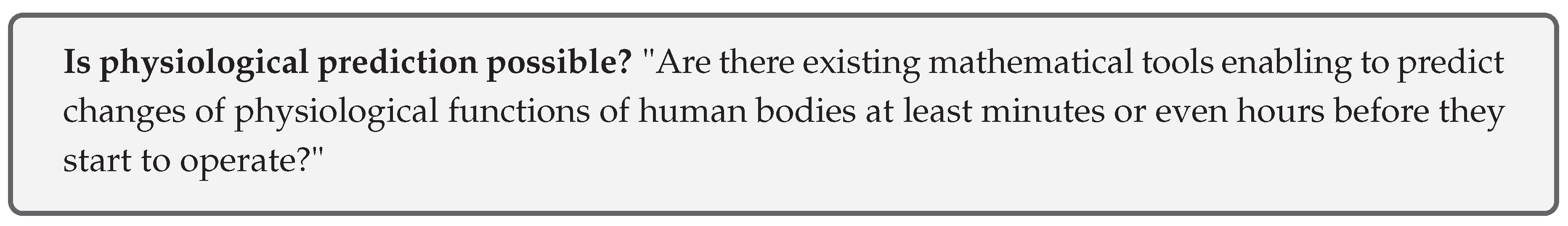
Throws of three dice give richer outputs; see Figure 1 for three selected examples: 1+1+1, 2+6+6, and 1+3+5 and their combinations. Only the first case (A), 1+1+1, is a pure macrostate. The other two cases in figure (B and C) are subsets of all microstates belonging to macrostates 14 and 9, which contain in total 15 and 25 microstates, respectively (see Table 2).
Figure 1 demonstrates three basic cases: all dice have identical output (they are dependent), two got identical output, and all three give independent results. The number p defines the chance of finding a specific configuration for a given case, and the number N defines the total number of possible outcomes. As the degree of independence rises, the number of possible outcomes substantially increases. Cases with higher independence contain all cases with lower independence.
There are shown some outcomes that belong to three different macrostates (sums) and selected microstates; examples are shown in Figure 1: (A) , (B) , and (C) . Only case (A) shows all microstates. Cases (B) and (C) contain total 15 and 25 microstates instead of the in-the-figure-shown 3 and 6, respectively; for details, see Table 2.
The complete list of all macro- and microstates is provided in the Table 2, where an obvious tendency of central sums to explode in the number of microstates is occurring. With an increasing number of dice, N, the central region of the macrostates that contain the majority of microstates gets narrower—it means that majority of dice throws will fall in this region.
When the change of distribution of #-of-microstates with respect to all possible macrostates for three to ten dice is depicted in a graph (see Figure 2; values are rescaled to make values comparable), there is present an evident tendency of shrinking the region of most often visited macrostates located around the center of all macrostates.
To demonstrate that the principles developed on dice throws can be easily applied to any other physical situations, an example with velocities having eight different directions of particle movements is shown in Figure 3. We can easily substitute directions with numbers, use eight instead of six numbers, use ’eight-sided dice,’ and study such cases exactly as we did with dice previously.
3.4. Entropy Definition in Statistical Physics
As we already know from Section 3.2, there is no way to deeply understand the very principles of the 2nd thermodynamic law from within thermodynamics itself because it treats heat as a continuum. The 2nd-TL is understood as the absolute law. Within thermodynamics, it is the absolute law as the entropy of an isolated system only increases there.
Ludwig Boltzmann overcame this difficulty [69,70,71,83] in his seminal research on the kinetic theory of gasses; gas is treated as a collection of atoms there. It was, for this period of time, a revolutionary concept of quantization of physical matter and properties!
The mathematical foundations of kinetic theory of gases—developed by Boltzmann—are covered by mathematics demonstrated in the previous Section 3.3. Statistical entropy —is a measure of the number of specific realizations of microstates [84]—and is defined by the Boltzmann formula [85] in the form
where is the Boltzmann constant and W is the number of microstates attainable by the system. This formula was derived under the assumption that states of the gas are quantized equally according to a function of momentum ().
As already mentioned, the definition of Boltzmann entropy relies on the atomic structure of gas and, in general, on the discreteness of the studied phenomenon.
It is easily seen that entropy is proportional to the amount of missing information. More indistinguishable microstates leading to a given macrostate means greater uncertainty (a constant system gives , whereas white noise, where all states are visited equally, gives ). The importance of this formula lies in the fact that it can be used not only in physics but also in communication, sociology, biology, and medicine. To be able to use this entropy formula, the following requirement must be fulfilled: all W states of the system (called in physics the micro-canonical ensemble) have to have equal probabilities. In such a case, it leads to probabilities (for all ). Entropy described in Equation (2) can be rewritten using this assumption into the following form
When the condition of equal probabilities is not fulfilled, an ensemble of micro-canonical subsystems is introduced with the property that within each th of the subsystems all probabilities are equiprobable. Averaging Boltzmann entropy under those assumptions leads to Gibbs-Shannon entropy
where defines averaging over probability p. Such derivation of Gibbs-Shannon entropy is often seen in textbooks [86,87]. This entropy is commonly used in statistical thermodynamics and in information theory; see the next subsection for details on information entropy.
Let us briefly review the historical development of the mathematical formulation of entropy [69,70,71,83] as it can be applied in other research areas, including biology & medicine, when understood correctly. Firstly, Boltzmann derived the H-theorem dealing with molecular collisions of atoms, which decreases in isolated systems and goes towards an equilibrium (it is also called the minimum theorem). Secondly, he proved that any initial atomic configuration reaches an equilibrium with time. This equilibrium approaches a specific distribution of atomic velocities, which depends on temperature, and is called the Maxwell-Boltzmann distribution.
Kinetic theory of gases explained the notion of pressure and temperature contrary to all previous continuous approaches. Additionally, Boltzmann proved that Quantity H behaves similarly to entropy except for a constant! His ideas were perceived as too revolutionary by his colleagues for the given level of understanding of physics. He had been repeatedly attacked by many leading physicists in his era. Their reason was an assumption that perfectly reversible atomic movements cannot lead to the irreversibility of H quantity!
A big fight was focused around the following discrepancy: deterministic movements of atoms leading to reversibility of their movements versus stochastic irreversibility of their ensembles. Boltzmann poured even more oil in the fire when he said that -TL is not absolute and in some cases entropy can spontaneously decrease from purely statistical reasons—exactly as we saw in the Section 3.3. He said, "most of the time entropy increases but sometimes decreases, and hence, -TL is not absolute." His work became a cornerstone of the foundations of modern physics and, subsequently, many other scientific disciplines, including biology. It gave impetus to the quantization of quantum physics.
3.5. Entropy Definition in Theory of Information
The notion of information was introduced by Claude Shannon to quantitatively describe the transmission of information along communication lines [45,46]. This concept later become useful in other scientific disciplines: linguistics, economics, statistical mechanics, complex systems, psychology, sociology, medicine, and other fields. It was shown by Shannon that entropy known from statistical physics is a special case of information entropy (often called Shannon entropy).
Figure 4.
(Left) Balls can help us understand the amount of missing information (which is equal to entropy): (A) All balls are same, which leads to zero entropy (1 config). (B) 3+1 balls have higher entropy (4 configs). (C) 2+2 balls give the highest entropy (6 configs). It is seen from the numbers of depicted, possible configurations. (Right) One square of a chessboard made of squares is hiding one nugget of gold. How many questions do we need to find out where it is hidden by splitting the region into two parts repeatedly? We need exactly six questions—it means six bits of information—while using splitting in halves. Otherwise, we need more.
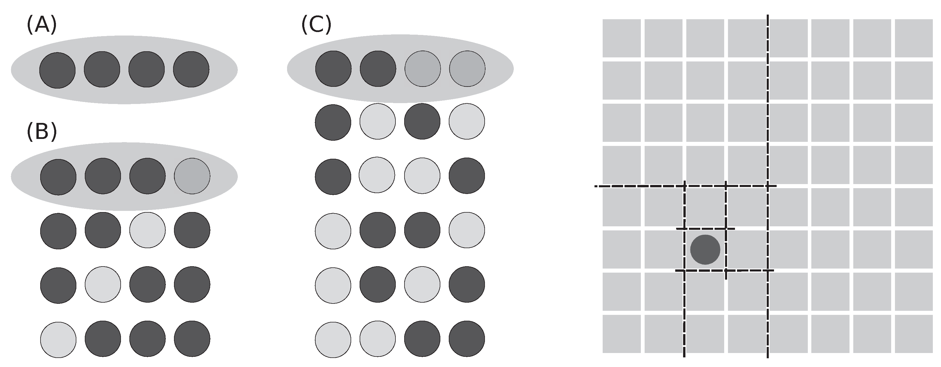
Let us introduce the amount of missing information on one example. We have a chessboard with squares where one square is hiding a golden nugget. The problem is to localize a given square by giving questions. What is the best strategy to find it? It is possible to guess which square is hiding the nugget. It might take up to 63 questions to find it: not so good a strategy. We can divide the board into two unequal parts and ask which one is hiding the nugget. It is definitely a better strategy: in the worst case, the output is approaching the speed of the previous case. What about halves? Yes. When we split the board into decreasing halves, the fastest localization of the nugget is found. It takes just steps to arrive at the final result each single time!
From this explanation, it is easily seen that the amount of missing information is equal to the number of questions necessary to localize information. As shown above, the gain from the smart way of questioning is maximal. Gain of information is one bit. Maximal information gain is in the case when two parts are equal. Contrary to it, asking one square after the other requires a tremendous number of questions.
Shannon entropy where probabilities of all W events are equiprobable, gives the following formula
There are W events, each having a probability of , giving . This can be simplified by making sum over equiprobable states that leads to .
Shannon entropy where probabilities of events are unequal must be split into different parts having the same probabilities that lead to the following formula
In this case, the sum cannot be removed from the formula as is done in the previous case.
In the seminal work of Shannon [45,46], the measure of the amount of information contained in a series of events was derived under the assumption that it satisfies three requirements:
- should be continuous in the .
- When all are equally probably, so , then is increasing function of N.
- should be additive.
This led to the famous Equation (6) because the above-provided assumptions yielded only this formula.
Information entropy and its applications are described in the following publications [29,30,36,37], where the topic is discussed with different levels of background requirements and where many examples are shown. Shannon entropy and its relationship to many scientific disciplines deserves more space, which we do not have here, because it is representing the root concept that is very useful in complex systems and many other disciplines.
3.6. Applications of Information Entropy in Biology and Medicine
As we already know, many natural systems, including complex ones, are beyond our capabilities to trace all their constituting parts in every detail. It was found that such tracing is not necessary for the correct description of macroscopically observed responses in complicated systems that acquire tremendous numbers of microstates. The concept of entropy demonstrated itself as very useful in the description of complex systems, in which detailed knowledge of their microstate configurations is not necessary for the description of macroscopic behavior. The usefulness of this approach was confirmed in the description of physiological processes operating within the bodies of animals and humans [13].
The obstacle in employment of entropy in description and prediction of biological systems is our insufficient ability to produce mapping of the complex system into the bins used in entropy. We must be able to find the best possible way of doing this mapping. None of the developed entropy measures is perfect—each of them has own pros and cons. There exist many approaches enabling the measurement of the complexity observed in biomedical systems using various types of information entropy: ApproxEn [13,38,39], SampEn [13], PeE [40], multiscale entropy [15,41,42], and others [28,43]. Permutation entropy (PeE) is used in this study to acquire data that are distributed in bins; see detailed explanation in Section 6.2.
4. Results–Part 1: Comparison of ’Normal’ with ’Non-TdP + TdP’ Rabbits
This section deals with the following grouping of tested rabbits: Torsades de Pointes (TdP) and non-TdP arrhythmia-acquiring rabbits (called arrhythmogenic) are included within one group, which is compared with the second group of rabbits that do not acquire any arrhythmia (called normal). Beware, later, in the next Results Section, see Appendix C, non-TdP arrhythmias acquiring rabbits will be excluded, and hence, only rabbits acquiring TdPs with those non-responsive (normal) will be compared there: discussion section will explain the details. Hence, it is necessary to be careful in comparing those two results sections!
Inclusion of both sub-groups in one group is done because ECG changes are expressing very similar features (definition follows) in both cases: TdP and non-TdP arrhythmia. A feature is defined as a measurable characteristic or property of the observed phenomenon. The selection of the most important features is crucial for building a highly predictive model. Simply said, we can suspect that all those rabbits showing double or triple subsequent PVCs—ectopic activity originating in the ventricles—can acquire TdPs, VTs, or VFs in the next hours or days. Authors of the experimental study [52] did not test this possibility (it was personally discussed with [88,89] by J.K. several times.) Firstly, in both cases (TdP and non-TdP) are displaying similar changes of T-waves: their broadening and increase of the amplitude that become comparable to the height of QRS complexes. Such morphological changes of ECG recordings are present a long time before the onset of a TdP arrhythmia; their presence is crucial. Secondly, TdP and non-TdP arrhythmia express a very similar pattern in the generation of double or triple subsequent PVCs at the stage where the T-wave becomes broad and high. This gives a consistent picture of the onset of an unstable substrate within the heart’s wall that is triggering twins (bigemini activity) and triplets (trigemini activity) of premature ventricular contractions (PVCs), which are sometimes called extra-systoles, because they are not preceded by an atrial contraction.
The search for the best mathematical method capable to visualize changes on ECGs capturing the development of TdPs was from the very beginning aimed towards the application of entropy measures of the original, unfiltered signals; see Section 2 and Section 3. This phase took the longest time as it was necessary to develop a wide and deep overview of complexity in medicine—the result is covered and reviewed in [63,68] and serve as an introduction onto this research. Permutation entropy [56] was selected as the most suitable entropy that can be applied to this problem. Immediately after the evaluation of permutation entropy, it was evident that outputs are very rich in information. Unfortunately, as was expected and shown later in this section, common statistical methods [76] applied by J.K. failed to reveal hidden correlation between computed permutation entropy and presence/lack of arrhythmia. Hence, it was decided to apply machine learning (ML) methods to automate the entire process of the best hypothesis search; see Section 2 for the motivation; see Table 3 for a brief description of all tested approaches.
The research done on finding the best up-to-date ML methods, which are capable of predicting arrhythmia with the highest scores, was very thorough, wide, and deep [90]. Authors decided to provide this information as a part of the paper for methodical reasons. It can enable everyone to conduct similar research in other areas of the biosignal processing, where ML methods might become more successful compared to the application of common statistical techniques. The sequence of all steps performed during the search for the best ML methods is explained in Section 4.8 and depicted in the picture in Appendix A.1. In order to enable the reader easily orient in the search, this section has the following structure: description of major types of arrhythmia, permutation entropy evaluation algorithm, permutation entropy () of rabbit ECG recordings, selection of sub-intervals of , feature selection, simple and advanced statistics, ML experiments, and ML results.
4.1. Description of Major Arrhythmia Types as Seen on ECG Recordings of Humans and Their Curves: TdP, VT, VF, and PVC in Contrast with Normal Ones
To provide a medical perspective to this position paper, real human ECG recordings: normal, Torsades de Points (TdP), ventricular tachycardia (VT), ventricular fibrillation (VF), and premature ventricular contractions (PVC) are presented in this subsection. Rabbit ECG recordings look quite similar.
A reliable prediction of life-threatening arrhythmias is the question of life and death in many cases; for example, heart diseases, guarding consciousness of professional drivers and airplane pilots, sportsmen, or hospital settings. In the following are presented samples of different types of naturally observed arrhythmias as observed on ECG recordings of humans along with the respective changes, if any exist, on PeE curves. This enables even non-specialists to visually recognize those serious, life-threatening arrhythmias; see their brief description in Table 4 and depictions in Figure 7, Figure 8, Figure 9, and Figure 10. Make sure to compare those arrhythmia recordings with the sample of the normal ECG recording Figure 6.
Figure 5.
A schematic depiction of one heart beat as seen on an ECG recording. The sequence of P-QRS-T is divided as follows: P-wave represents contraction of atria, QRS-complex contraction of ventricles, and P-wave repolarization of ventricles (repolarization of atria is covered by QRS complex). The normal ECG recording of a healthy rabbit is shown in Figure 6.
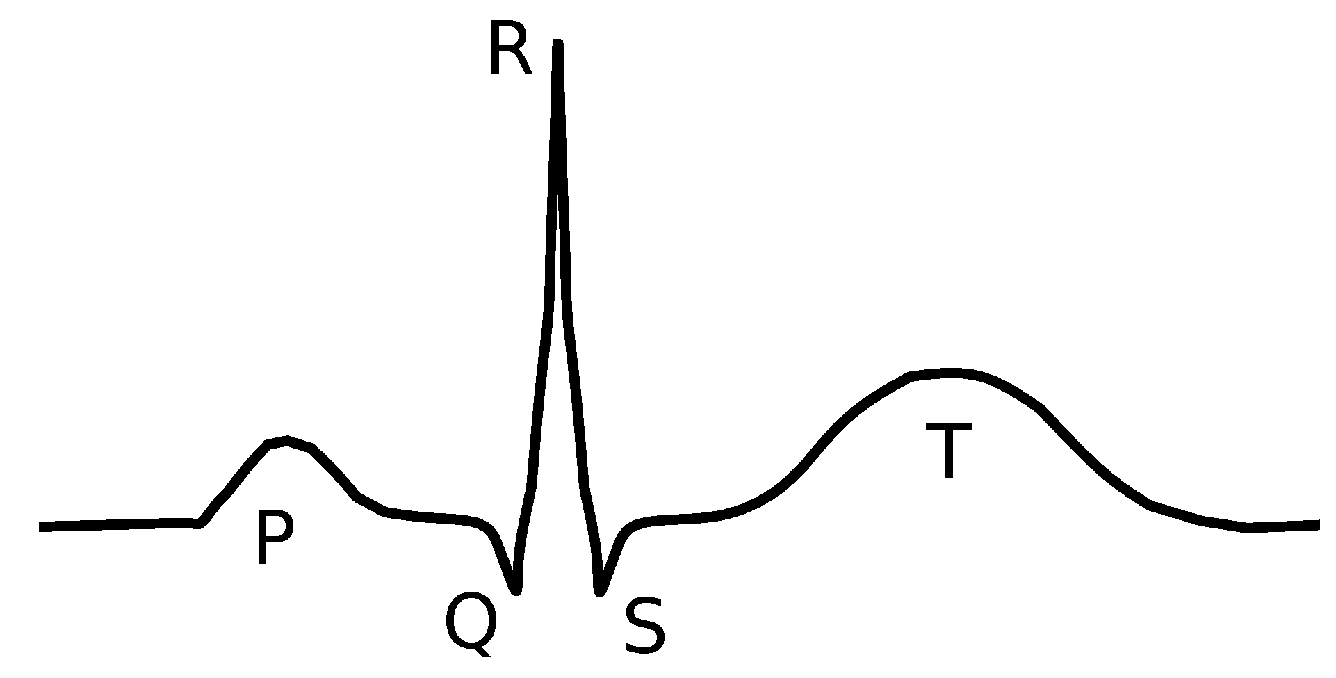
To make a good reference ECG curve, Figure 6 depicts the case of the standard ECG recording of a healthy person, which is called in the following text the normal ECG recording. It clearly shows the standard sequence of atrial contraction (P-wave), ventricular contraction (QRS-complex), and ventricular repolarization (T-wave). The schematic depiction of a normal heart contraction, as observed on ECG recordings, is depicted in Figure 5.
Figure 6.
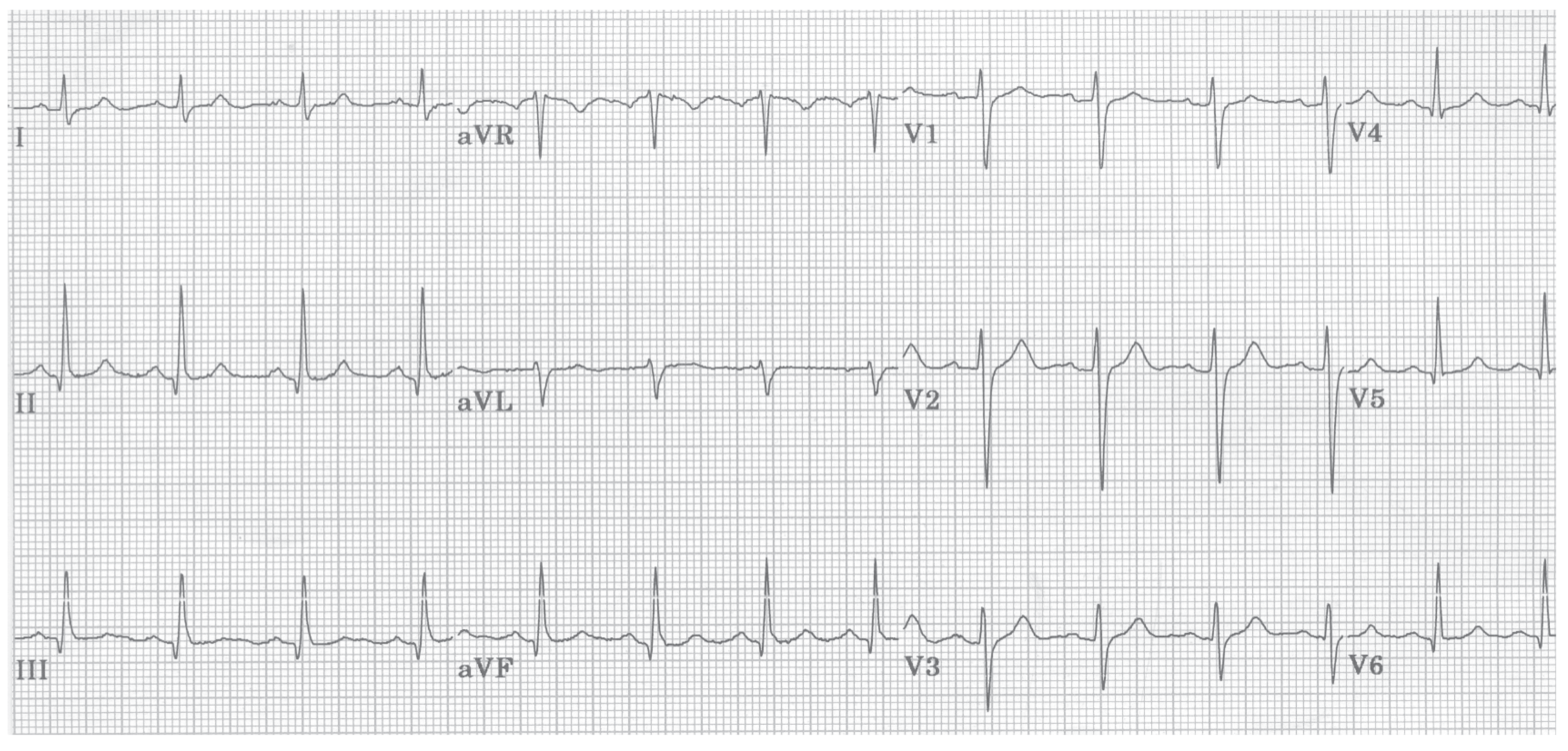
A normal ECG recording of a human is providing the baseline to all arrhythmias shown in the subsequent figures. A normal ECG curve always contains a P-wave, a QRS complex, and a P-wave. All the subsequent graphs, which are depicting arrhythmia recordings, show distorted ECG curves; courtesy of [91].
Figure 6.
A normal ECG recording of a human is providing the baseline to all arrhythmias shown in the subsequent figures. A normal ECG curve always contains a P-wave, a QRS complex, and a P-wave. All the subsequent graphs, which are depicting arrhythmia recordings, show distorted ECG curves; courtesy of [91].
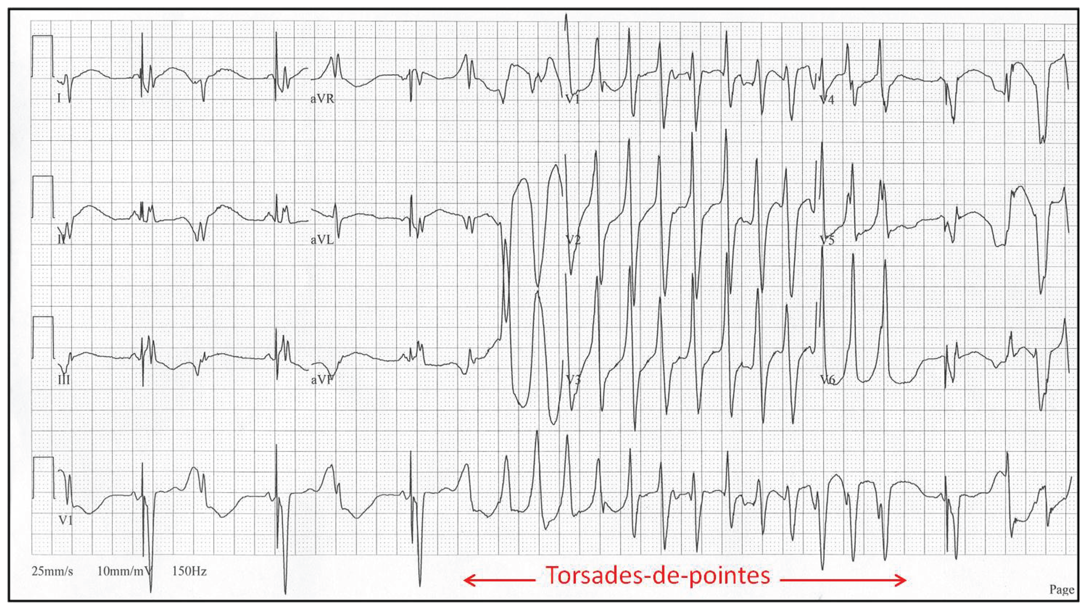
Torsades de Pointes arrhythmia is typically triggered when the QT interval, which is measured between Q and the end of the T-wave, exceeds a certain threshold; in humans, it is 500 ms. In such cases, it can happen that partially recovered cardiomyocytes after excitation can be excited again. This leads to the occurrence of an unnatural, meandering pacemaker focal point in ventricles instead of in the atrium, which subsequently triggers an arrhythmia that is quite often fatal.
Figure 7.
Torsades de Pointes (TdP) arrhythmia of a human, which is typically induced by drugs, both medical and recreational, affects the functioning of ion channels that, in turn, change the propagation speed of the action potential through cardiomyocytes. As seen from the figure, ECG recordings have sinusoidal shape of the envelope following the maxima of the ECG curve. TdP often degenerates into a life-threatening VT or VF; courtesy of [91].)
Ventricular tachycardia is typically triggered by either morphological disturbance(s) or by dispersion of velocities of action potential propagation through ventricles; it has normally shape of a distorted sinus curve. It triggers self-sustainable excitable focus that replaces the natural pacemaker located in the atria. Frequencies of VT typically lie within the range of 130-250 bpm. With increasing frequency of VT, ejection fraction of expelled blood from the heart decreases substantially. Above 200 bpm, such arrhythmia when generated in ventricles is typically classified as ventricular fibrillation by automatic defibrillators despite it still being a VT run. Ventricular fibrillation is seen as an uncoordinated, random noise on ECG recording.
Figure 8.
An ECG recording of ventricular tachycardia (VT) of a human looks like a deformed sinusoidal curve (due to aberrated QRS-complex) of fixed maximum height. The heart’s ejection fraction (the volume of ejected blood) is substantially decreased during VT; an affected body can cope with such arrhythmia for some period of time but often does not; courtesy of [91].
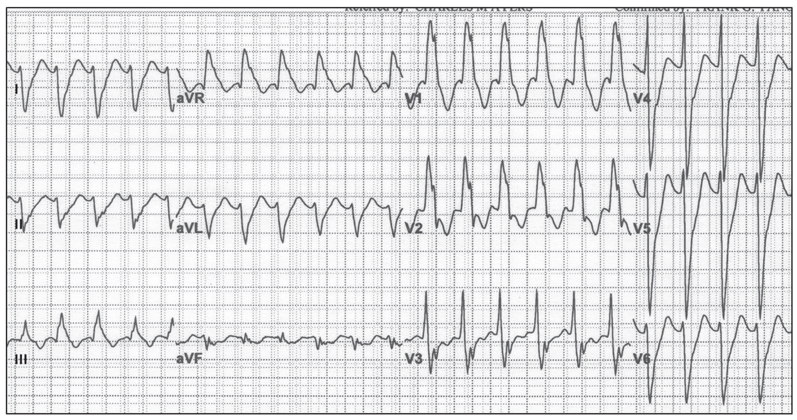
Figure 9.
During a ventricular fibrillation (VF) of a human the ECG recording is randomly going up and down in a completely uncoordinated fashion. The heart’s ejection fraction is reaching zero value during VF and quickly leads to a condition incompatible with life; courtesy of [91].
Figure 9.
During a ventricular fibrillation (VF) of a human the ECG recording is randomly going up and down in a completely uncoordinated fashion. The heart’s ejection fraction is reaching zero value during VF and quickly leads to a condition incompatible with life; courtesy of [91].
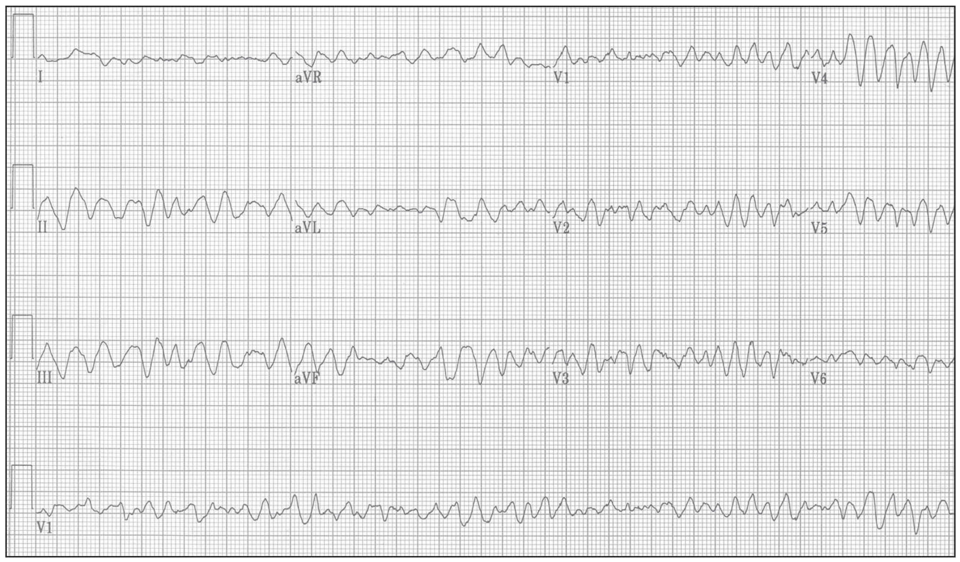
Figure 10.
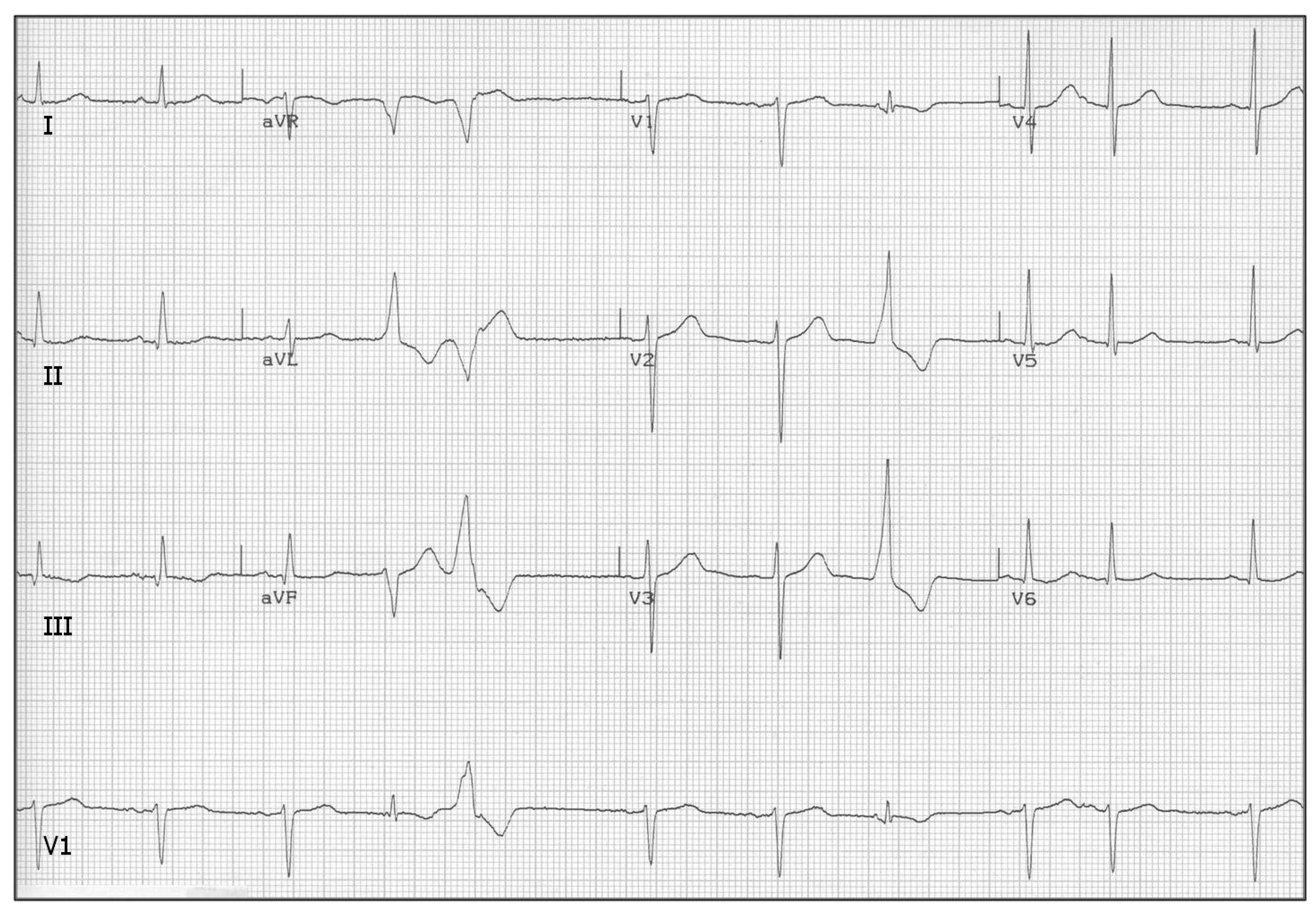
Premature ventricular contractions (PVC), a.k.a., extra-systoles, look like a single oscillation of a VT run with a missing P-wave. Actually, replacement of SA-node pace-making activity by an ectopic center(s) in ventricles is the same in both cases. PVCs occur sporadically even in healthy people; courtesy of [91].
Figure 10.
Premature ventricular contractions (PVC), a.k.a., extra-systoles, look like a single oscillation of a VT run with a missing P-wave. Actually, replacement of SA-node pace-making activity by an ectopic center(s) in ventricles is the same in both cases. PVCs occur sporadically even in healthy people; courtesy of [91].
4.2. Algorithm and Graphic Depiction Describing Evaluation of Permutation Entropy: Allowing Easy Orientation in Following Results
For a better understanding of the role that permutation entropy (PeE) is playing in deciphering hidden processes that are operating within complex systems, it is necessary to acquire a basic understanding of the PeE evaluation. For this reason, the following brief introduction to PeE is provided. The rigorous definition of PeE is found in Section 6.2.
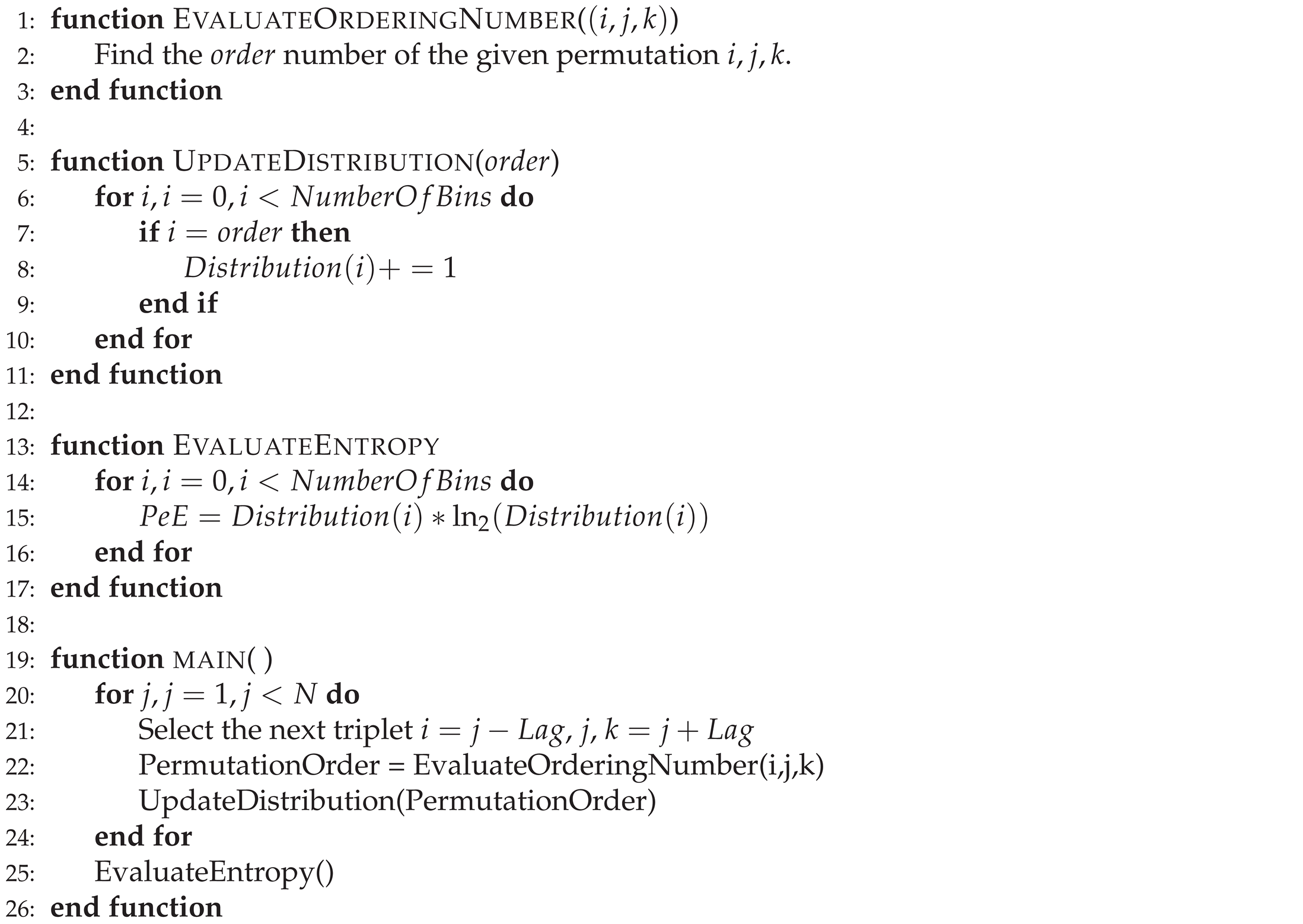
Figure 11 depicts the evaluation of a single value of permutation entropy using three points. Each of those evaluated values is added to the relevant bin of the PeE distribution, where the number of bins is equal to the total value of permutations (in this case, it is equal to six, ). Finally, PeE is evaluated using this distribution.
The principle of PeE evaluation is described at Algorithm 1 in the form of a pseudo-algorithm whereas the code itself is found at [92]. The Python code contains a main function, evaluation of the single value of PeE, evaluation of the ordering number, and update of the distribution.
| Algorithm 1 The algorithm that is evaluating permutation entropy, which uses three points with the distance equal to , is described using a pseudo-code [92]. N is the length of the input string; triplets of points; the variable defines the distance of values between points of triplets; the variable represents the number of bins within the distribution. |
 |
4.3. Permutation Entropy () of Rabbits’ ECG Recordings
Permutation entropy, [56], is normally applied to R-R intervals (the distance in [ms] measured between two R peaks of the subsequent QRS complexes) to reveal hidden dependence of R-R variation and a given disease (cardiomyopathy, arrhythmia, or sleep apnea [18,55], etc.). Traditionally, R-R intervals are processed in order to remove PVC beats, which are replaced by some local, averaged value of R-R. In HRV studies, ECG recordings might be preprocessed by filtering and other signal preprocessing tools to achieve ’clean’ curves. The novelty of the presented approach lays in the fact that we do not use any kind of preprocessing at all and do study the full ECG recordings. ECG recordings are used in their native form without a change of even a single bit (e.g., it can be checked by use of a visualization software [93]). The idea behind it is quite simple: in this way, we are not losing any valuable, hidden information about underlying physiology—hence, we keep all hidden information from the underlying complex system within the evaluation process.
Two sets of curves with varying L-s (10, 20, 30, ..., 90, 300) are shown for typical arrhythmogenic (Figure 12) and non-arrhythmogenic (Figure 13) rabbits, respectively. The full set of L-s (representing the distance between measuring points of triplets in [ms], details in Section 6.2) encompasses: 10, 20, 30, ..., 90, 100, 200, 300, and 500 [ms]. In some cases, the abbreviation is used, where #L stands for the measure L. There is present an apparent dependence of curves on the drug application times for the typical arrhythmogenic rabbit, and a lack of this dependence for the typical non-arrhythmogenic rabbit. The problem is that this behavior can be swapped, in a minor number of cases, for unknown reasons, i.e., an arrhythmogenic rabbit can express the response that is visually close to a non-arrhythmogenic one and vice versa. We are unable to distinguish those two cases visually and using statistics, as it is necessary to simultaneously compare fourteen projections of each single ECG recording into different with varying L-s. Additionally, there are 37 different ECG recordings.
Observations achieved during the initial stages of entropy evaluation that are briefly summarized in Figure 12, Figure 13 and Figure 14, along with a number of standard statistical evaluations, led to the hypothesis that there are existing hidden relationships between curves and the presence/non-presence of arrhythmia. It was found that simple statistical measures such as mean, variance, standard deviation (STD), min/max differences, and slopes of curves cannot discriminate arrhythmogenic rabbits from those non-arrhythmogenic—this is the moment where a lot of research using standard statistical approaches ends [95,96,97].
The next natural step is to apply modern machine learning methods (ML) [8,9,47,48,49,50,51,63] that are becoming routinely used in such situations. Whenever there exists a hidden relationship among data that is impossible to reveal by standard approaches (equations, statistical methods, etc.), ML methods are often capable of finding such missing relationships.
4.4. Preprocessing of ECG Recordings: Detailed Inspection of ECG Recordings, and Defining Exact Moments of Drug Applications and Their Increasing Doses
The moments of application of medical drugs (anesthesia, methoxamine, and dofetilide), along with their increasing dosages for every single tested rabbit, were carefully put into a table. This was later utilized in defining the appropriate segments of ECG recordings that were used in the ML experiments. This table made by (J.K.), along with all ECG recordings [52], is not part of this study. The original drug application times are stored in [52].
4.5. Statistical Features of Subintervals: Demonstrated on Selected Example of 20
The first natural step in finding hidden dependencies and relationships among experimental data is the application of all standard and advanced statistical methods to uncover them [90]. Unfortunately, according to previous non-systematic testing (J.K.), it appeared that data resisted revealing any reasonable dependence between the presence/non-presence of an arrhythmia in rabbits and the shape of curves using statistics; it was anticipated due to the works of other researchers that failed for the same reason (using HRV studies [52]). The best achieved sensitivity and specificity of decisions of the presence of arrhythmia using statistics from curves was about 75% in the best cases, which is not sufficient for any effective clinical predictions.
Examples of those observations are documented on two selected sub-intervals of 20 (control and methoxamine), which are giving the best results from all computed results. To demonstrate those facts, two box plots are shown in Figure 15 and Figure 16. Figure 15 shows the five most important statistical features for the control sub-interval of the 20 curve of all rabbits (arrhythmogenic rabbits are in blue and non-arrhythmogenic rabbits are in red). Figure 16 displays the identical situation but this time for the first methoxamine sub-interval. Evidently, the discrimination between arrhythmogenic and non-arrhythmogenic rabbits is impossible using statistical features. As already said, it was the moment where most, if not all, studies end. The question was, “Is possible to go further and find hidden dependencies among data?” This possibility is demonstrated in the rest of this section.
After a thorough inspection of the presented data in Figure 15 and Figure 16 and all other cases of PeE#L (with #L going from 10 up to 500), it became evident that yet another modern, more sophisticated computational approach must be used to reveal information that is scattered among many PeE#L curves and their features simultaneously. This approach is called machine learning (ML)—an important part of the AI research area—which is gaining increasing popularity among researchers processing physiological and other medical data. ML often succeeds in finding dependencies among measured and preprocessed data in situations where all statistical methods fail.
Machine learning is represented by many algorithms and computational methods—regression (the oldest one), decision trees, random forest, support vector machine, clustering, ensembles, neural networks, etc. [9,35,47,48,49,50,51,63]—that are used to reveal hidden data dependencies, which are not being possible to describe by equations, curves, or statistical methods.
4.6. Systematic Definitions of All Features Used During Preprocessing and Evaluation of Curves: This Section Serves as Reference to all Experiments Conducted in This Study and To Easy Orientation
4.6.1. Definition of Data, Features, and Used Operators Abbreviations: Systematic Overview
A large number of features were tested during the search for the best ML methods that can predict the occurrence of arrhythmia; see Table 5. To allow everybody to follow all tested cases easily, a clear and concise abbreviation of all feature combinations was developed; those abbreviations were used consistently within all evaluations presented in the following subsections and tables. The abbreviations are covered in this subsection.
Each feature abbreviation has the following structure; it consists of the following three parts: <data part><symbol><feature part>. The features that are specified in the feature part are evaluated using data specified in the data part. The <data part> contains the following abbreviations: OC = original curve, SI = sub-intervals, M = merged (M is used before SI), I = isolated (I is used before SI), and the attribute RM = rolling mean.
The <symbols> used in the description of each feature abbreviation (definitions above and below): "_": separates data and feature parts (e.g., ISI_Top5-TM); "-": represents the logical relation inside both data and feature parts of the abbreviation (e.g., ISI-DFT_Top5-C); "&": merges together features computed on the left and right sides of this operator (e.g., ISI_Top5-TM & ISI_ASF). The priority of evaluation of symbols is the following: ’-’ > ’_’ > ’&’. It starts with the symbol of the highest priority, ’-’, and ends with the symbol ’&’ of the lowest priority.
The <feature part> can contain the following symbols: -L = values of the L parameter, _Top5 = top five, *SI-DFT = s reconstructed by discrete Fourier transformation (DFT) approach, *SI-DWT = s reconstructed by discrete wavelet transformation (DWT) approach, *SI-D*T_Top5-C = top five coefficients (D*T = DFT or DWT), -TM = time moments, -SSF = simple statistical features, and -ASF = all statistical features (simple + advanced).
An example of the use of the abbreviations follows: MSI_Top5-TM = Merged Sub-Intervals_Top 5-Time Moments; see Table 5. The operator "-" is left-associative, it is meaning that the operations are grouped from the left. An example is that gets interpreted as .
4.6.2. Assessing Curves and Designing Data Structures for ML-Experiments
Each rabbit was subjected to a number of drug infusions, which were applied at different times and had different durations. Such data cannot be compared directly. It is necessary to reflect those variations in the data evaluation and comparison by making an appropriate data preprocessing. Data had to be properly shifted and sliced to enable their comparison. Shifts were done according to the times when the respective drug infusion was applied (methoxamine and dofetilide I-III, -). Drugs had been applied continuously after each infusion initiation: they were not mere boluses. Therefore, the following data exploration steps were performed:
- (i)
- The minimum number of drug infusions that was common for all rabbits was selected in order to compare rabbits correctly. It yielded two intervals: the interval ’0’, called the comparison/control interval (before ), and the interval ’1’, called the methoxamine one (after ). No other intervals can be used because some rabbits got arrhythmia and expired during the second interval (after the application of the first infusion of dofetilide, ; the interval called ’2’). Yet some other rabbits died at the interval ’3’, after an increase of the dose of dofetilide, . Whereas, all non-arrhythmogenic rabbits survived all harsh drug insults applied.
- (ii)
- For each rabbit, a selected control interval had the length of 505 seconds (the minimal common value) just before the application of the first infusion (methoxamine). The actual moment of methoxamine application, , vary for all rabbits.
- (iii)
- Time intervals between the moment of initiation of methoxamine infusion , , and the first dofetilide infusion, , are different for each rabbit, and they yield . Firstly, the length of this interval is retrieved for each rabbit separately. Secondly, the minimal common length of this interval for all rabbits was assessed, which produced the value of 465 seconds. It is assumed that the moment of methoxamine application, , belongs to the interval of methoxamine and not to the control interval—the drug disruption of physiology starts there, whereas anesthesia disruption is already present in the control interval.
4.6.3. Preprocessing of Curves: Design and Creation of Subintervals That Were Subsequently Tested by Whole Range of ML Methods
According to the previous section dealing with the data exploration, two intervals were dissected from each curve control and methoxamine that are abbreviated and called control (’0’) and methoxamine (’1’), respectively. In the following, the term ’value’ is used, which represents an interval having length of 5 seconds. curves were exported by averaging over this interval because the actual signal oscillates too much when displayed at each point of the original ECG recording within each [ms]). The lengths of the original curves have between 550 and 1416 values (2750 and 7080 seconds). According to the previous, 101 values (505 seconds) were taken for the control interval and 93 values (465 seconds) were assumed for the methoxamine interval. The maximal lengths of control and methoxamine intervals are defined by their respective maximal common lengths in all curves. Remember, from now on we work only with evaluated s and not original ECG recordings.
It is necessary to take into account the rounding process that might have an influence to results, but which size is difficult to assess. Obviously, drug infusions started in arbitrary moments. Due to this fact, the initiation times of drug infusions were rounded to the nearest lower value, which is a multiplication of five seconds (141 to 140, 14 to 10, 88 to 85 etc.).
4.7. List of All Tested Combinations of Features Used to Find the Best Statistics and ML Methods: This Serves as Thorough Navigation Tool to Design Similar Future Approaches
This subsection briefly describes why features are so important and also provides an overview of all used features along with their mutual combinations in this study (details in [90]). Generally, each evaluation of data using ML methods goes from simple features to the more advanced ones. Combinations of features are used in the case when everything else fails. The necessity to use features extracted from the original data in ML methods is manifold: (i) original data are too huge, (ii) original data are not suitable to apply ML methods on, and (iii) there is a need to describe data by some special features not present in the original data (slope, maximum, mean, SD, entropy, information content, etc.).
4.7.1. Simple Statistical Features
Simple statistical features used in this study are represented by mean, standard deviation, variance, min, max, 25th, 50th, and 75th percentiles. Those are standardly used statistical features.
4.7.2. Advanced Statistical Features
Advanced statistical features used in this study are represented by: integral, skewness, kurtosis, slope, , energy of time series, sum of values of time series, and trend of time series (uptrending, downtrending, or without trend).
4.7.3. All Tested Features and Their Combinations
Control and methoxamine sub-intervals were cut from all curves for all rabbits using a special procedure; see the preprocessing above (Section 4.4 and Section 4.6.3). Those sub-intervals were and the original PeE curves were used to compute all features—see Table 5 for a list of all used features and their combinations—which were applied in the search for the best methods for predicting arrhythmia. To enable an easy orientation among all features, a visual guidance is provided. The importance of each set of features (which are acquired during subsequent evaluation) is reflected by the number of stars (more star symbols equals more important results). Results are grouped into the following groups: ’***’ as best (ARARS ≥ 90%), ’**’ as sufficient (80% ≤ ARARS < 90%), ’*’ as average (75% ≤ ARARS < 80%), and ’ ’ as not useful (no star) (ARARS < 75%); see the Equation (9) for the definition of ARARS score.
4.8. List of All Performed Machine Learning Experiments: The Core Part of the Conducted Research Together with Permutation Entropy Evaluation
This is one of two essential parts of the whole research conducted and covered in this paper (see details of ML experiments in [90]), which is intentionally made very detailed and deep for methodical reasons. The entire search algorithm is shown in Appendix A.1 in the form of a map depicted in Figure A1. The main reason behind all of this is to provide enough procedural knowledge to all who would like to apply similar research in their respective field of signal processing—not only in biology, but also in any scientific field working with signals (physics, sociology, economy, etc.). This thoroughness helps non-specialists to realize the full capabilities of ML methods in not only biosignal processing.
- (A)
-
Important time moments: each of s sub-intervals was too long for ML methods (approximately 100 values), and thus various subsampling strategies were tested: only Random Forest succeeded. The pitfall in this approach is that the classification outputs were—in this way—introduced to the experiment already during the subsampling process by Random Forest. After this preselection, the identified important time moments (subsamples of the sub-intervals) were used—served as the input—for subsequently used ML methods. It is not sure whether this approach can be considered an allowable one when we deal with such an extremely low number of ECG recordings.To confirm the achieved results of this preselection, the importance of the identified time moments was manually verified by Box-and-Whisker plots (box plots). It was revealed that arrhythmogenic and non-arrhythmogenic rabbits have different values (distributions) at these time moments, and thus we validated the correctness of identified features. This implies the fact that the same time moments could be identified manually. It is done by comparing the values (distributions) of arrhythmogenic and non-arrhythmogenic rabbits at the appropriate time moments. Thus Random Forest may be interpreted just as a selection technique helping to automate and speed up the selection process of the important time moments.There is still existing a possibility of failure of this approach on larger data. The reason is that the important time moments were identified on a few s and may not exist in the case of the larger data set, number of ECGs—see Figure 17 for a counter-example where an example similar to our case is represented by five sinus curves where the conclusion is subsequently negated by use of ten curves—and thus use of this type of feature is extremely unsafe, and the achieved results must be considered with extreme caution!The identified important time moments of the sub-intervals were tested by:
- (i)
- single machine learning algorithm and
- (ii)
-
ensembles of them
- (1)
- Bagging
- (2)
- AdaBoost
- (3)
- Combination of different algorithms for each value of L parameter
- (4)
- Combination of classifiers (see Section 6.5) for all values of L parameter at once
- (B)
-
Simple statistics: the simple statistical features (mean, standard deviation, variance, min, max; 25th, 50th and 75th percentiles) were evaluated and then tested using the following ML methods & features
- (i)
-
Simple statistics of the original s
- (1)
- (dead end) by a single machine learning algorithm, and
- (2)
-
(dead end) by ensembles of them
- (a)
- (dead end) Combination of classifiers for all values of L parameter at once.
- (ii)
-
Simple stats of the sub-intervals
- (1)
- (dead end) by a single machine learning algorithm, and
- (2)
-
(dead end) by ensembles of them
- (a)
- (dead end) Combination of classifiers for all values of L parameter at once.
Wherever the words ’dead end’ are used, it means that the given ML method(s) did not reach any significant result. - (C)
-
Advanced statistics: advanced statistical features (integral, skewness, kurtosis, slope, [max-min]/length of , energy of , sum of values of , trend of [uptrending, downtrending or without trend]) were evaluated and subsequently tested together with simple statistical features using the following ML methods
- (i)
-
Simple + advanced stats of the original s evaluated by
- (1)
- (dead end) by a single machine learning algorithm and
- (2)
-
by ensembles of them
- (a)
- (dead end) Bagging,
- (b)
- (dead end) AdaBoost,
- (c)
- (dead end) Combination of different algorithms for each value of L parameter,
- (d)
- Combination of classifiers for all values of L parameter at once.
- (ii)
-
Simple + advanced stats of the sub-intervals evaluated by
- (1)
- (dead end) by a single machine learning algorithm and
- (2)
-
(dead end–all following cases) by ensembles of them
- (a)
- Bagging,
- (b)
- AdaBoost,
- (c)
- Combination of different algorithms for each value of L parameter,
- (d)
- Combination of classifiers for all values of L parameter at once.
- (D)
-
Important statistics: important statistical features from the simple + advanced stats were evaluated and subsequently tested using the following ML methods
- (i)
-
For the original s
- (1)
- (dead end) by a single machine learning algorithm and
- (2)
-
by ensembles of them
- (a)
- (dead end) Bagging,
- (b)
- (dead end) AdaBoost,
- (c)
- (dead end) Combination of different algorithms for each value of L parameter,
- (d)
- Combination of classifiers for all values of L parameter at once.
- (ii)
-
For the sub-intervals
- (1)
- (dead end) by a single machine learning algorithm and
- (2)
-
by ensembles of them
- (a)
- (dead end) Bagging,
- (b)
- (dead end) AdaBoost,
- (c)
- (dead end) Combination of different algorithms for each value of L parameter,
- (d)
- Combination of classifiers for all values of L parameter at once.
- (E)
-
Statistic & Time Feature Combinations: Combination of statistical features (simple + advanced or only important from simple + advanced) and important time moments were tested using the following ML methods:
- (i)
- A single machine learning algorithm and
- (ii)
-
Ensembles of ML Algorithms
- (1)
- Bagging,
- (2)
- AdaBoost,
- (3)
- Combination of different algorithms for each value of L parameter,
- (4)
- Combination of classifiers for all values of L parameter at once.
- (F)
-
DFT coefficients: Important DFT coefficients of the sub-intervals, selected from the first 15 real and first 15 imaginary DFT coefficients, were tested using the following ML methods:
- (i)
-
A single machine learning algorithm (k-NN)the best result found for 40 is giving: Se = 0.845, Sp = 0.835, AUC = 0.840, Acc = 0.839, and
- (ii)
-
Ensembles of ML algorithms
- (i)
- Combination of classifiers for all values of L parameter at once.
- (G)
-
Important time moments based on DFT: important time moments of the sub-intervals reconstructed by the first ten DFT coefficients (real and imaginary parts) were tested by:
- (i)
- (dead end) by a single machine learning algorithm
- (H)
-
DWT coefficients: The ten most significant DWT coefficients in absolute value of the sub-intervals were taken. These coefficients were sorted in descending order for subsequent classifying using machine learning algorithms by
- (i)
- (dead end) A single machine learning algorithm,
- (ii)
-
Ensembles of them
- (1)
- Combination of classifiers for all values of L parameter at once.
- (I)
-
Important time moments based on DWT: important time moments of the sub-intervals reconstructed by the ten most in absolute value significant DWT coefficients were tested by
- (i)
- A single machine learning algorithm.
- (J)
- Useful L: best values of L parameter based on all above-mentioned experiments. This section contains the summary; see Table 8 values of the L parameter with ARARS scores greater than 80%. In the case of values of the L parameter with ARARS scores greater than 90%, their highest ARARS scores are explicitly stated. As can be seen from the table, the most useful values of the L parameter are 10, 90, and 500.
- (K)
- The usefulness of ML methods and their best results has been evaluated and documented; see Table 7.
- (L)
- Outlier detection was not performed due to an insufficient number of experimental ECG recordings.
- (M)
- Real-time prediction on the one-minute sub-intervals was tested. It revealed that the first three minutes after application of methoxamine are the most important.
4.9. List of Best Achieved Machine Learning Results for Normal Group Against non-TdP and TdP Acquiring Group of Rabbits
4.9.1. Lags L of That Are Giving Best Results for Listed Combinations of Features and Algorithms
4.9.2. Predictions Employing Majority Voting above Simultaneous Combinations of Classifiers for All Values of Lags L
This ensemble approach used combinations of ML algorithms and all available information (i.e., s from different drug intervals and of different values of L parameter) in order to make a final prediction by majority voting. Additionally, each algorithm used only those values of the L parameter that achieved an ARARS score of at least 75% for the used algorithm.
The Table 7 lists achieved results where the process map IDs provide the navigation keys to the items in Section 4.7.3, which is providing the detailed list of all tested features. The values of L parameter, which were used for prediction, may be found in the Table 6.
The fourth line from the bottom in Table 7 displays the following, very important, abbreviated information—Features: ISI_Top5-ASF, Process map ID: 3dii2d, Applied ML algorithm: SVM, Sensitivity = 0.93, Specificity = 0.93, AUC = 0.93, and Accuracy = 0.93. It has to be read as: an ensemble of SVM algorithms was applied above isolated sub-intervals (control and methoxamine) with selected top five from all tested statistical features and that all above all curves and all lags L. This ensemble is giving the following output: Sensitivity = 0.93, Specificity = 0.93, AUC = 0.93, and Accuracy = 0.93.’

Table 7.
Results were achieved by the application of the ensemble approach where a combination of from 3 to 32 (identical or different) ML algorithms (see column ’Used Algorithms’) applied to preselected features (see column ’Features’) originating in the curves for two different intervals (control and methoxamine). The final prediction is reached by application of the majority voting using the given ensemble. Only classifiers (ML methods) with ARARS > 75% were used in ensemble learning. Abbreviations Se, Sp, AUC, and Acc stand for sensitivity, specificity, ROC area under curve, and accuracy, respectively. Process map ID provides the navigation key in Section 4.7.3.
| Features | Process map ID | Used algorithms | Se (%) | Sp (%) | AUC | Acc (%) |
|---|---|---|---|---|---|---|
| ISI_Top5-TM | aii4 | SVM | 1.0 | 1.0 | 1.0 | 1.0 |
| RF | 0.99 | 0.88 | 0.93 | 0.95 | ||
| k-NN | 0.99 | 1.0 | 0.99 | 0.99 | ||
| LR | 0.96 | 0.87 | 0.91 | 0.93 | ||
| OC_Top5-ASF | di2d | SVM | 0.83 | 0.97 | 0.9 | 0.88 |
| SVM, RF, k-NN, LR | 0.8 | 0.99 | 0.9 | 0.87 | ||
| OC_ASF | ci2d | SVM | 0.83 | 0.86 | 0.84 | 0.84 |
| ISI_Top5-ASF | dii2d | SVM | 0.93 | 0.93 | 0.93 | 0.93 |
| ISI_Top5-TM & ISI_Top5-ASF | eii4 | SVM, RF, k-NN, LR | 1.0 | 1.0 | 1.0 | 1.0 |
| ISI-DFT_Top5-C | fii | SVM | 0.99 | 0.99 | 0.99 | 0.99 |
| ISI-DWT_Top10-C | hii | SVM | 0.95 | 0.85 | 0.9 | 0.9 |
Why is this specific output so important? We hypothesize that the main reason is in the fact that ensemble voting is performed above all available curves and both intervals. It was not tested, but very probably those results will be close to deep learning (DL) results. The reason DL and an ensemble of SVM algorithms will give similar results is their huge flexibility in distilling the underlying, hidden data interdependencies within the original ECG recordings and hence, in all curves too.
The human brain is simply unable to keep in so much different information at once for so long time—hundreds of curves for different lags for minutes—contrary to the above-mentioned algorithms. The complexity of the underlying complex system—the body physiology plus the heart condition—is beyond our comprehension. Computers using appropriate algorithms can accomplish this feat easily.
4.9.3. List of Best ML-results for All Values of Lags L: Guide to Easy Orientation
This section contains a summary (see Table 8) of the most useful values of the L parameter for given ML methods that are giving ARARS scores greater than 80%. When values of L parameter with ARARS score are greater than 90%, their values are explicitly displayed. It can be easily inspected from the table that the most useful values of the lag L parameter are 10, 90, and 500.
Table 8.
The list of the most useful values of the lag L parameter for given ML methods that are giving an ARARS score of at least 80% (symbol ’x’). All ARARS values greater than 90% are provided with their numerical values explicitly.
Table 8.
The list of the most useful values of the lag L parameter for given ML methods that are giving an ARARS score of at least 80% (symbol ’x’). All ARARS values greater than 90% are provided with their numerical values explicitly.
| L | ||||||||||||||||
|---|---|---|---|---|---|---|---|---|---|---|---|---|---|---|---|---|
| 1 | 5 | 10 | 20 | 30 | 40 | 50 | 60 | 70 | 80 | 90 | 100 | 200 | 300 | 400 | 500 | |
| RF | x | x | x | |||||||||||||
| SVM | x | x | x | x | x | x | x | 0.92 | x | 0.92 | x | 0.93 | ||||
| k-NN | x | x | x | x | x | x | 0.92 | x | x | x | 0.91 | |||||
| LR | 0.92 | 0.92 | x | x | x | x | ||||||||||
| Ensemble | 0.95 | x | x | x | 0.92 | x | x | 0.93 | ||||||||
5. Discussion
This publication is focusing on three major directions: (a) research results, (b) a detailed review of applied methods, and (c) a detailed discussion of all pros and cons of the used methodology. The combination of all parts enables everyone to better understand and subsequently apply the used methodology in biomedical and other research areas where complexity measures in combination with ML methods could be applied. The results and the entire methodology are supported by the rich citation apparatus.
The discussion starts with the introductory subsections defining the hypothesis creation in statistics and ML (Section 5.1), input data access and reliability (Section 5.2), which is deepened in a thorough, very important discussion of ’reliability, reproducibility, and safety of ML/AI solutions’ (Appendix B) defined in [98]. The following parts are focused into three distinct areas: complex systems (Section 5.3), machine learning (Section 5.4–Section 5.7), biomedical part (Section 5.8), and it is ending with the future directions (Section 5.9). All of those parts are focusing on different aspects of the same problem and are mutually complementary. Additionally, this structure helps specialists in the field of ML quickly reach the core message (jump to Appendix B). Other parts offer an easier penetration into the subject to nonspecialists using different concepts of thinking and terminology.
5.1. The Role of Hypothesis Creation and Testing in Science, Statistics, and Machine Learning
Hypothesis creation and testing is playing a great role in science [95,96,97,99]. To make the entire subject of the hypothesis creation process more clear, we review three distinct types of hypotheses used in science & research:
- (i)
- A scientific hypothesis is a preliminary idea/guess fitting the evidence that must be further elucidated [95]. A good scientific hypothesis is testable, and it either proves itself to be true or false. When it is proven true, then it becomes a law or theory. In the future, any law or theory could be disproved in the light of new evidence.
- (ii)
-
A statistical hypothesis is dealing with the relationship between observations. A statistical hypothesis test is used to compute a critical value (called p) that says how probable it is that the observation is by mere chance [95]. Lower p means a higher probability that the observation is not by chance due to the chosen data. High p means that relationship is probably observed by chance. The value means that chosen hypothesis can be valid by mere chance in five percent of cases—with decreasing p, such chance decreases. We are never one hundred percent sure about the outcome of statistical hypothesis testing, even for very small p-values. That is why we want to reach a p as small as possible.Two types of hypotheses are used:
- (0)
- Null hypothesis–H0 means that there is no difference between observed events with some value of p. No effect is present.
- (1)
- Alternative hypothesis–H1 means that we suggest the presence of some effect. The alternative hypothesis is accepted when the null hypothesis gets rejected.
- (iii)
-
The machine learning hypothesis is a model that approximates the relationship between input and output in the best way from all possible hypotheses that can be made using a given method(s) [48,78]. Learning in ML is de facto searching through the space of all available hypotheses for a given set of ML methods.There are two types of hypotheses recognized in ML
- (1)
- h (hypothesis): It is a single hypothesis. A specific model is mapping inputs into outputs, which can be evaluated and used to make predictions on unknown data.
- (2)
- H (hypothesis set): It is a space of hypotheses. A space of all possible hypotheses, which can map given inputs into known outputs, that is searched through for the best candidate.
By choosing model(s) and its parameters, we define a hypothesis space H, which is searched, that contains a single hypothesis h that will best approximate the targeted function between inputs and outputs. It is more efficient to choose more models and parameters, as it speeds up the search time. This is a very difficult task, as we do not know the target function in advance.
5.2. Input Data: What We Must Be Aware of Prior to Evaluation of ECG Data by Entropy Measures and ML Methods
What kind of data should be provided to data scientists/mathematicians that will enable them to carry out deep and reliable research above those data? How do those data get checked and processed prior to applying entropy measures, after it, and prior to applying ML methods?
- (i)
- Availability of ECG recordings as open access data has a very high priority in research. This is the fundamental condition of development: availability of reliable & replicable AI, ML, and DL methods in medicine. Everyone must be able to reevaluate the research (data are not open-source in this study [52,88,89]). Additionally, it opens the development to the future even more sensitive algorithms and their easy comparison with their predecessors. Each change of the ECG database (usually its update) must be followed by reevaluation of the actual and all older algorithms applied to it. It can be automated.
- (ii)
- Annotation of ECG recordings by cardiologists. This gives very strong input data to all supervised algorithms/methods that are going to be applied on those data, as it ensures that the methods will provide correct outputs. Any errors in ECG annotation can be fatal to all subsequent evaluation steps of ECG recordings. Those errors must be avoided prior to any further evaluation of data; a double-check by using two different approaches is desirable (not done above ECGs from this study).
- (iii)
- Visual inspection of ECG recordings by a mathematician prior to their CS processing. It enables decreasing the possibility of spoiling training data by incorrect data. This is hard, as mathematicians are usually not trained to classify heart arrhythmia, tachycardia, blocks, and other heart diseases, but failure in this stage can save serious, unwanted consequences on data processing. Completely nonsensical data can be ruled out in this way. Exclusion of data must be carried out with great care, as we might rule out some features that we currently do not understand but in the future they can be found useful.
- (iv)
- Entropy measures evaluation of ECG recordings. To carry out the visual inspection of entropy curves is necessary. HRV variability inspection is desirable too, as it can reveal the presence of some hidden, non-obvious physiological insults that can influence the development of classification/prediction methods. Within the ECG recordings used in this study, there were detected abrupt changes of HRV that were not explained by their authors. A detailed inspection of entropy measures that are present in combined graphs reveals a lot of hidden information, and it helps to design the ML phase of the research and improve feature selection.
- (v)
- Statistical evaluation of entropy curves serve as a preparatory step for the application of ML methods. Statistics alone are unable to discern and classify observed phenomena and provide sufficient preciseness and reliability.
- (vi)
- Feature selection. It is important to pre-process data, as they are usually too large to be evaluated by ML without any kind of feature selection. Feature selection narrows the amount of processed data in the ML stage.
- (vii)
- Machine learning preliminary tests. This stage helps to quickly scan huge space of all tested hypothesis that are defined by input data and their statistical processing, which produces features used in ML methods.
- (viii)
- Machine learning production runs using various methods. This stage is zeroing in on the final, most efficient ML methods above given input data. A very important part of this stage is the application of different ML methods above the same data that can, in the ideal case, be preprocessed differently. Identical outputs from different ML methods are strong evidence that the methodology and the effect itself are correct.
5.3. Complex Systems View: Wider Background and Methodology
Living systems represent one of the most complicated complex systems known to science. They are, by definition, except in some special cases, very hard to understand, describe, manipulate, and predict using standard mathematical tools such as differential equations, chaos, statistics & probability, etc. [63,68]. Therefore, the application of statistical methods to evaluate biosignals generated by human bodies is almost always unsatisfactory—because they often fail to distinguish various cases (e.g., arrhythmia vs. normal rhythm). Simply said, statistics do not capture emergent processes and emergent processes and entities—that are operating within all living systems; see more in the following.
For example, HRV analysis can be performed by using only statistical methods. Unfortunately, this approach is not applicable for the prediction of TdP arrhythmia. In our study we are using two groups of rabbits: arrhythmia-susceptible (arrhythmogenic) and normal (non-arrhythmogenic). Arrhythmogenic rabbits acquire either TdP arrhythmia or non-TdP arrhythmia, such as PVCs or double or triple PVCs. To distinguish those two subgroups—normal and arrhythmogenic—automatically means that we have to use some other, more advanced mathematical tools than mere statistical methods.
Such situations occur quite often in biomedical research, where hidden dependencies among data remain unrevealed or, even worse, an incorrect dependence is found [95,96,97]. Why is it so? Any biosystem can be viewed, using a certain level of abstraction, as a very complex network of dependencies and relationships in a functional sense and even in a topological sense (networks of amino acids, proteins, cells, tissues, etc.); see Network Biology and Medicine [100,101,102]. Hence, a biosystems’ fingerprint in the form of a biosignal is a by-product resulting from those interactions and dependencies—where the exact location of the system’s subtle changes remains mostly indistinguishable from biosignals.
Further, to make things even more complicated, those networks react to changes, which are originating in a signal coming from its one part, as a whole. Going back to our study, there exists a distribution of velocities of action potential propagation across the heart wall, which is normally homogeneous. We can think in terms of a substrate. Each time, when the substrate changes its properties dynamically—becomes an-isotropic in action potential propagation velocities—it is effectively masking its inner changes against observation. Unfortunately, statistical methods are unable to detect such processes. In general, any change in any part of the biosystem is masked due to numerous dependencies and links in the rest of the system.
Is there any escape from this trap? The answer is "Yes, there is a solution that was already developed in statistical physics in the description of complicated physical systems containing a large number of mutually interacting constituting parts." It got a name: entropy [45,46,69,70,71,83]. Entropy when applied wisely to biosignals often helps to reveal hidden dependencies even where statistical methods fail. Entropy, enables a deep penetration into the inner functioning of the system, by a dramatic reduction of the complexity of the information content of the original system. Often, this information reduction/compression is much higher than that produced by statistical methods when applied to the same data.
Generally, each complex system occupies a certain number of different microstates—which is usually an insanely huge number. Those microstates are reflected in one macrostate. There are present many such macrostates that are by orders of magnitude lower than the total number of all possible microstates. The concept of entropy helps to create groups of those microstates that are achieving the same macrostate. It simplifies the complexity of studied systems dramatically, but it still can help to discern different major modes of their behavior. The rigorous explanation of this approach requires a deep understanding of statistical physics [45,46,69,70,71,83]; see Section 3. It is necessary to be aware of the fact that this process is based on a kind of compression of information contained in the original system, and therefore, it is prone to errors. This means that two distinct microstates having different properties can fall into one macrostate and become indistinguishable.
Figure 18.
The whole research procedure is displayed in one figure: (a) The original system—the human body—is located at the top. Going in the clockwise direction: (b) biosignals & data are extracted from the body, (c) those biosignals are treated as complex systems data using complex systems measures (permutation entropy), (d) statistical methods are applied to data retrieved by complex system measures, and (e) finally, AI & ML methods are applied to statistical data. A refined cycle can repeat.
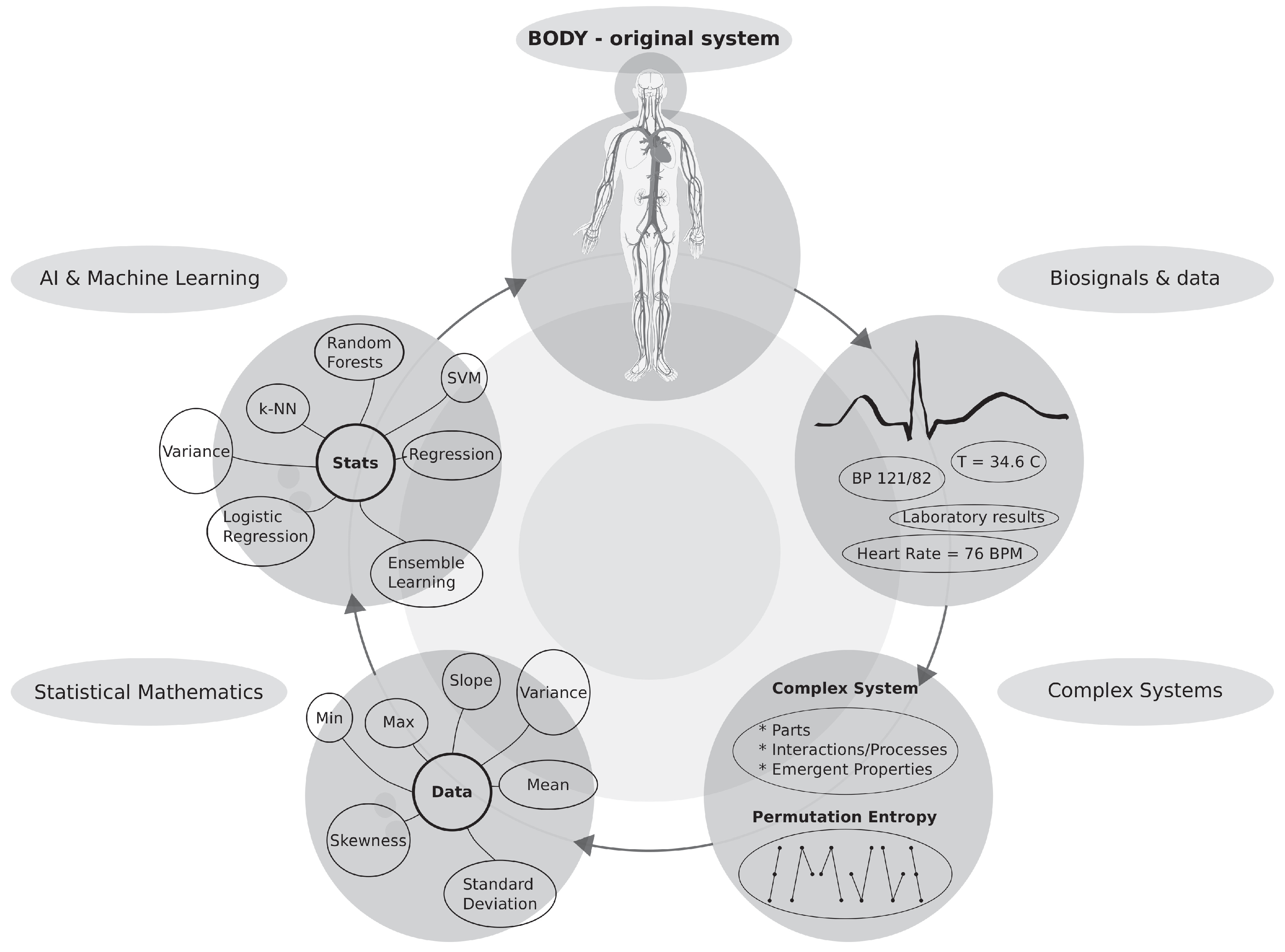
While thinking about the description of biosignals in this way, a question might be raised: "How many dependencies unrecognized by any of the classical approaches will experimental data reveal after going through the above-mentioned process?" Machine learning (ML) methods have proven themselves as a very useful toolkit. Generally and very roughly said, ML methods are capable of tracing subtler changes present within data in many features simultaneously in ways that are inaccessible to human perception, standard mathematical tools, and statistical methods. It represents a kind of highly distributed perception that is inaccessible to humans.
5.4. Machine Learning View: Grouped by Different Approaches
5.4.1. Classification by statistical features of alone
It was demonstrated that the classification of arrhythmias up to one hour before its onset reached its highest value at about 75% sensitivity or specificity, when the classification was performed using single statistical features. Obviously, it is not a satisfactory result for reliable use in hospital and home care. Here, in the next step, a principal change in the applied methodology used to search for dependencies among data occurs quite naturally. This methodology is commonly applied in search for hypotheses that are describing data relationships.
5.4.2. Single ML Methods
The next natural step in arrhythmia classification was to apply ML methods. Results got better when compared to simple and advanced statistical methods alone. The classification reached its highest value at about 85% of sensitivity or specificity when it was performed using single ML methods.
5.4.3. Ensembles of ML Methods: statistical features, selected times, and other features
A completely different situation occurred when ensembles of ML methods were used to classify arrhythmia in rabbits; see Table 7 in Section 4.9.2. An ensemble of SVM methods succeeded in achieving 93% sensitivity and specificity in the prediction where the top five features from all statistical features of sub-intervals (ISI_Top5-ASF) were taken into account. This is a rather unexpected result: the mere combination of important statistical features classifies arrhythmias with such high sensitivity and specificity. Different SVM classifiers are uniquely combined within an ensemble to achieve 93% (compare to values achieving a mere 75% and 85%; see the two Subsubsections above).
Yet another approach was tested—it is not expected to be reliable enough by the authors—when important time moments were preselected see Section 4.8 and Figure 17. The time moments are selected by RF method, and thus the output of one ML method was used as an input of the other ML method (SVM or k-NN in this case). Ensemble of SVM method and ensemble of k-NN-method reached more than 99% of sensitivity and specificity for top five time moments on isolated sub-intervals (ISI_Top5-TM). Beware, this approach is less reliable due to too few evaluated cases (rabbits). Hence, RF can find combinations of moments that will not be confirmed on larger numbers of animals; see both subfigures in Figure 17. The combination of all statistical features and the top five time moments (ISI_Top5-ASF and ISI_Top5-TM) yielded 100% for ensembles where SVM-, RF-, k-NN-, and LR-methods were used.
The top five coefficients of discrete Fourier transformation gave 99% sensitivity and specificity (ISI-DFT_Top-5-C) as well. This observation supports the independent observation provided by SVM and k-NN provided above. Again, as in the previous case, in the cases where two ML methods are applied sequentially on such small data, we are in danger of huge overfitting to small data. Only testing of this approach on larger data can tell us more.
5.5. Advantages of Used ML Methods
ML methods represent a still relatively underestimated set of tools enabling the uncovering of data dependencies that are unavailable to classical methods (such as equations, statistics, and probability). They provide a capability to reveal so-far inaccessible internal data structures and flows, and they are representing prospective hypotheses creating tools. To the surprise of many researchers, advanced ML techniques open doors to much simpler methods once they reveal complicated, hidden interdependencies among not obviously related data. Some of those hypotheses lead to discovery of hidden laws. The used words ’not obviously related data’ are crucial for the possibility of application of simpler methods. Specifically, those simpler methods can discover some not-so-obvious ’shortcuts.’ In other words, once a given dependence is found (using advanced ML-techniques), we know where and for what to look. In this way, a much simpler method (possibly statistical or a simple single ML method) can become the workhorse of future data evaluation.
Let us go back to our classification of arrhythmia. Firstly, the curves were evaluated with lags for each rabbit, which express a rich response to applications of drugs. It was evident that some hidden relationship—with a complicated pattern that is not easy to discern—is present there as already shown but no statistical method using simple features found them. Application of ensemble ML methods successfully found a relationship among the very same data for various sets of selected statistical features.
It must be mentioned that ML methods are opening doors for even more advanced methods, which are known as data mining (DM) [49]. DM can help in their unsupervised mode to find even more convoluted dependencies among data. The knowledge about those dependencies can be used in simpler and computationally less expensive methods (statistics, ML) for standard use. Simply said, DM and ML methods can serve as a sieve that search through many possible dependencies among data quickly—i.e., they automate hypothesis testing [95,96,97].
5.6. Disadvantages of Used ML-Methods
Surprisingly, a big disadvantage of ML methods is the level of trust in them, which is quite low, originating in their relative novelty. Therefore, there is no sufficient penetration of knowledge about rules of their use, capabilities, and deficiencies [98]. Often, this is the source of incorrect applications of AI & ML methods in biomedical research and clinical practices, which originates in the lack of mutual understanding between mathematicians/data specialists on one side and medical doctors with biomedical researchers on the other.
The penetration of this knowledge is gradually improving, nevertheless, the biggest problem of ML methods lies unexpectedly within psychological and ethical issues. There is an ongoing big debate about whether the life of any patient should rely on ML methods or not. Often, questions about AI & ML sound like: "Can we trust an algorithm/machine?" The answer to this question is not straightforward. To a certain extent, it can be said that the situation is the same as in statistics, where trust in algorithms is present as well. Entire evidence-based medicine is based on the application randomized controlled trials (RCT) approach, which is nothing more than simple statistics. Actually, it is too simple to be capable of describing the whole complexity of human bodies and their reactions to therapies. An example from AI applications: we already use simple AI/ML methods in implantable defibrillators to estimate their possible charging using intracardiac electrocardiograms (IEGs) prior to more robust algorithms evaluating an arrhythmia and giving a go to an application of a discharge. An AI method produce an estimate that trigger the capacitor charging, which takes up to about ten seconds, while simultaneously a more robust algorithm further evaluates an event that is accompanied by anti-tachycardia pacing.
The other disadvantage of all methods trying to classify biomedical data (not only by ML methods) lays in scarcity of reliable experimental biomedical data and their open-source databases. Such a situation must be addressed by the decision-makers at the level of states. They should create mandatory open-access databases of biomedical data that will be used to test, verify, and calibrate all AI solutions applied in human medicine. No exception is allowed. Any failure in this verification will ban the application of a given medical method from its use. It will bring the safety of biomedical research to the level of the safety achieved in the aerospace industry, where the safety mission is already successfully implemented and achieved—it can serve as an example.
5.7. Limitations of Achieved Results: General and Specific
In general, the first and biggest limitation of this and many other biomedical studies is the notoriously small number of patients available in studies. This lack of biomedical data is not accidental. It is caused by difficulties with data acquisition due to: the low frequency of patients having a given disease, expenses related to acquiring data, and lastly, the necessity to allocate qualified MDs to classify and analyze them. In the case of animal studies, the necessity to buy animals that are studied in experiments—which must be from well-defined, expensive lineages—and to provide their required care brings additional expenses. Larger animal species require even greater expenses not only due to their size but also due to their longer life span.
Data used in this study [52,88,89] contains too few measured ECG recordings—only 37 in total for all normal and arrhythmogenic rabbits—to make it reliable. Due to data size, splitting arrhythmogenic curves into two groups, which was required by ML methods, brings the classification to the edge of the possible. There is a danger that the classification is imprecise. Nevertheless, such problems are encountered in most biomedical studies. This is one of the main reasons why all issues are discussed so deeply and from many angles.
Other very probable limitations of the study:
- Different species, such as rabbits, dogs, pigs, and humans, will very probably produce different features. Hence, ML methods will produce different results!
- The same species can have inter-species variability. It means that the same output, an arrhythmia, can have two distinct sets of features that detect it.
- For laboratory animals is more often observed lack of inter-species variability and signs of inbreeding. This shifts experimental animals far from the standard population that is having high numbers of gene alleles and different epigenetic setups!
- It is even possible that specially bred laboratory animals could produce different results in different laboratories for undecidable reasons, because some part of the protocol can be slightly altered, diet different, the treatment of animals by staff different, or the operation procedure can vary. One example can be a light regimen that strongly affects the hormonal setup of animals that are otherwise identical.
- All influences from the above can somehow—for us in unknown ways—alter the underlying physiology of the tested animals. This has a substantial impact on heart physiology of animals and, hence, can alter the entire experiment and arrhythmia prediction.
- The robustness of achieved results in this study must be tested by exploration of larger numbers of animals, different species, and finally on humans.
- A single AI/ML method is less reliable than several independent methods reaching the same conclusion. At this point it is worth stressing out that this research is consistent with deep learning research [103] results where authors found a neuronal network capable of predicting arrhythmias in ICU patients one hour before their onset from ECG recordings.
5.8. Biomedical Point of View
When bodies are observed as complex biological systems, everyone realizes that the past descriptions of those systems were highly insufficient and imprecise. Anyone starts to give himself a crucial question: “What is the best way to describe the level of complexity of a system we are observing?” Because the inability of scientists to detect and/or model all subtle details and processes undergoing in cells, tissues, organs, and bodies is well known, therefore, some kind of simplification of this huge complexity must be applied. A generic answer, which was developed to solve a very similar problem in physics, can be found in one-and-a-half-century old research of statistical physics applied to gases: entropy [69,70,71,76,83]—see Section 3 and Section 4.3 for details.
Reasoning of this kind leads directly to the methodology applied in this study, where a two-step approach was applied. In the first step, the full-blown complexity is computationally compressed by applying an entropy developed specially to describe the complexity of biosignals: permutation entropy [56,57] (see Section 6.2 and Section 4.3 for definitions). In the second step, the manual search—performed by a researcher—for a complicated relationship among complexity measures (taken as inputs), and predictions of the presence/absence of arrhythmia (taken as outputs) is avoided by employing automatic methods of creation & testing of hypotheses between input and output data. Those methods are called AI & ML (Section 4 and Appendix C).
This reasoning enables capturing at least some of the in-the-hierarchy-of-emergents operating emergent structures, whose presence is interwoven within the complexity of the actively operating system. Signatures of emergent structures are reflected in biosignals. Once the emergents present within the system disappear—which cannot be directly observed due to the immense complicated nature of the observed system—this situation is externally expressed as a complexity decrease of the biosignals that we can observe. Exactly such complexity decrease is observed in ECG recordings prior to and during arrhythmia, as shown in this study. According to the results of this study, it is a positively confirmed fact that a decrease in the complexity—measured by the permutation entropy—of the properties of the underlying heart substrate/tissue is reflected in ECG recordings and correlates with a decrease in the permutation entropy of ECG recordings. The goal is manifold: to detect this decrease automatically, discern it from other possible causes of complexity decrease, and do all that with sufficient sensitivity and specificity.
Detected entropy changes of the initial system state are at the beginning very subtle—that means they cannot be detected by the naked eye—but they increase with decreasing complexity of ECG recordings with the limiting cases of TdPs, VTs, and VFs, where the computed complexity decreases substantially compared to the initial, healthy state. In this way, AI & ML can ’see’ subtle changes within biosignals, well before any trained cardiologist is capable of recognizing an incoming catastrophe in the form of deadly arrhythmia—it is mostly due to the fact that AI evaluates entire five-minutes-long intervals containing many beats at once for many s simultaneously. With a certain simplification, we can speak about an ’AI microscope’ that is capable of analyzing subtle changes in biosignals and predicting incoming events. Whether such predictions will occur as vital and will eventually be applied in medicine must be thoroughly tested on large databases of ECG recordings; see Appendix B for details.
A two stage approach, which uses complexity & AI/ML methods to look for a deeper insight into the observed complex system (here, human physiology of the heart), has greater chances to capture subtle changes within the observed system, unlike the direct application of simple and advanced statistical methods on original ECG data. Once such a deeper insight is captured, it provides a basis enabling better understanding of the underlying processes that are not directly observable. Additionally, the proposed approach brings a possibility to discover hidden subgroups of two main groups: arrhythmogenic and normal/non-reacting rabbits. It brings the study toward more personalized approaches, which enables delivering treatments to only those who will benefit from them. We can make such a decision prior to the onset of a long-term, potentially damaging therapy.
The entire study—when observed by an independent observer from the meta-level—shows a distinct pattern. Initially, complexity is reduced using an entropy measure. It is followed by a complete statistical analysis that has proven itself useless when used alone. The next natural step is to use AI & ML methods to uncover convoluted dependencies among statistical data and other observed features.
Statistics has been applied in biomedical research for a long time. Nevertheless, it has inherent deficiencies [95,96,97] that everyone must always be aware of. AI & ML methods are relatively novel approaches—not as widely used in biomedical research. It is going to change in coming years as they offer so far inaccessible possibilities in our description and understanding of phenomena observed in biomedical research; this is discussed in Appendix B in detail.
This brings us to the crux of the matter. The very definition of the scientific method is based on the creation of hypotheses that are falsifiable. In other words, each theory is developed with the intention to describe and predict the behavior of an observed natural phenomenon. Everyone can easily decide whether a theory describes a given phenomenon or not. Once a theory is derived—this part is hard—, it is relatively easy to test it. Initially scientific methods used numbers, later equations, algebra, geometry, calculus, differential equation, statistic & probability to describe dependencies among data. New methods always occurred when old ones had shown themselves insufficient to solve the latest challenges.
Development of new theories is becoming harder and harder with increasing complicatedness of described phenomena. A way to overcome this obstacle is the application of an automatic creation of hypotheses according to observed data. It is where AI, DL, ML, and DL algorithms (methods) become highly useful. AI and ML enable automatizing of hypothesis creation. Up to a recent time, it was an unheard-of procedure. Most of the scientists still highly underestimate the capabilities of AI hypothesis creation. Most importantly, AI is not the last possible stage of applicable, descriptive methods’ development. We must keep our ability to observe science from the above still open. It prevents of getting locked in a repetitive and fruitless application of just one type of method endlessly.
5.9. Future Directions
Obviously, the algorithm incorporating the methods used in this study can be—and very probably will be—applied to other animals and even to human ECG recordings (the software used to predict arrhythmia is provided as the open-source code under the GPL-v3 license [92,104]). The sequence of evaluation of & application of an ensemble of ML methods must be tested on much larger sets of ECG recordings. It is valid for a given species and given experimental settings. It would be very suitable to create a database of ECG recordings (a testbed) on which new algorithms and approaches predicting arrhythmia (not only this one type) can be easily tested.
Let us go deeper into the analysis of the used methodology. As mentioned before, achieved results do not have high statistical importance because there are not enough measured ECG recordings. Such situations where data are lacking are very common in medicine. Therefore, it is worth of studying and analyzing those situations in depth, as is done in this paper. This uncertainty can be only resolved by using much larger databases of ECG recordings. Nevertheless, acquiring of large ECG databases is a big problem because such ECG recordings capturing arrhythmia are scarce and require a large workload and often even large financial resources (for animals). Human ECG can be collected easily in ICUs of each hospital. Additionally, each research facility or hospital collects those data independently, which leads to the fragmentation of those databases and waste of scarce resources.
There are two possible ways that can resolve such a situation: (a) official and approved databases of ECG recordings and (b) databases created from data collected by wearable devices. Researchers can try to organize the creation of a joint database of ECG recordings gathered from wearable devices of various producers that are capturing arrhythmia—it will greatly benefit patients and even developers, as it will ensure a high standard of all developed AI & ML software tools. The first private company already released the AI software implemented in a wearable device—Apple Watch 4 [21]—that is capable of detecting and reporting atrial arrhythmia, as was tested by the Harvard study [105]. Something similar can be applied to TdP arrhythmia—it requires cooperation of different parts of biomedical research, hospitals, and private companies.
This study and other studies on sleep apnea [18,55], consciousness levels [106], gait classification of (pre-)Alzheimer patients [14], classification of anesthesia depth [16,17,107], epileptic classification [53,108], 3D image classification [109], atrial fibrillation [110], and other studies [42] are clearly pointing out that research based on entropy measures of complex systems in combination with ML methods is having a very promising future not only in classification of complicated physiological states but also in their prediction.
6. Materials and Methods
The main idea behind the ECGs’ evaluation presented in this paper is to work with the raw ECG recordings where no kind of preprocessing is applied. This approach enables tracing and capturing invisible details, trends, and information hidden within them. The methods applied to achieve this goal—that were applied subsequently—can be roughly divided into three distinct groups: permutation entropy, statistical features, and machine learning. Data preparation, evaluation, approaches, and methods applied within all evaluation steps are described in the following text in separate subchapters.
6.1. Database of ECG Recordings Measured on Rabbits
With respect to rabbits used to produce ECG recordings, animal handling was in accordance with the European Directive for the Procession of Vertebrate Animals Used for Experimental and Other Scientific Purposes (86/609/EU). All experiments performed on rabbits, including ECG recordings, were performed by D.J., L.N., and M.Š. [52,88].
All 37 ECG recordings were measured on rabbits where arrhythmia was induced by the subsequent continuous application of methoxamine and dofetilide infusion with gradually increasing doses of anesthetized animals (details [52]). Anesthesia was induced and maintained with a combination of ketamine () and xylazine () applied every 30 minutes. Anesthesia is influencing the heart activity as well. On ECG recordings, sudden bursts of HRV were observed at random places. We do not know the exact moments of anesthesia applications; hence, we can not tell more about those bursts. Therefore, the term ’control interval’ must be assumed with care when control intervals of rabbits that are getting implanted electrodes (no anesthesis) are compared to those with anesthesia. The baseline results might be quite different!
Prior to the application of methoxamine , approximately a 10 minute-long control interval was recorded where the given animal remained at rest. ECGs of all animals were measured at a minimum of 465 seconds after the application of methoxamine infusion and prior to the application of dofetilide infusion of . Dofetilide was added to the infusion of methoxamine; it could lead to a TdP arrhythmia. When no arrhythmia occurred dofetilide dose was increased to , which could lead to TdP arrhythmia for other animals. Some animals got the dose of dofetilide . After the application of those drugs, 1/3 of animals remained resistant to all drug infusions and did not develop any signs of arrhythmia [52].
All ECG recordings can be split into two or respectively, three groups. Two group divisions encompass rabbits that acquire arrhythmia (24 animals) and those without it (13 animals), where the arrhythmogenic group include both TdP and non-TdP arrhythmia. The second three-group division contains the following groups: non-arrhythmogenic (13 animals), non-TdP arrhythmia (10 animals), and TdP arrhythmia (14 animals). Due to a really high asymmetry of numbers of animals (ECG recordings) among three groups and simultaneously due to a few measured animals (only 37), initially, it was decided not to use a three-group split; hence, a two-group split was tested; see Section 4. Later, the modified two-split was tested too with grouped non-arrhythmogenic and non-TdP arrhythmia rabbits versus normal rabbits (details in discussion); see Appendix C. Two-split enabled the use of ML techniques with 10-fold cross-validation; details in the ML section.
Each recorded curve represents a single ECG channel that was digitized using 1000 samples per second and 24 bits per sample. The typical length of the recording is 120 min (7200 sec) with the following structure: each anesthetized animal is kept at rest on average for about 10 min (the minimum is 505 seconds), which is measured after adjustment of ECG leads (this period is called the control); methoxamine infusion is applied and kept unchanged on average for about 10 min or more (the minimum is 465 seconds); then the first dose of dofetilide is applied. Finally, whenever the rabbit does not acquire an arrhythmia, the next increased dofetilide dose is applied, and so on.
Within this study, only two intervals are taken into account: control and methoxamine. Dofetilide intervals were not taken into account for prediction because some animals acquired the TdP arrhythmia just after application of the first infusion of dofetilide. Inclusion of a finer grouping of arrhythmia would lead to a partitioning having even smaller groups of animals during evaluation of various ML methods—this deteriorates the reliability of results when the number of animals is small (our case) but increases their preciseness when animal numbers are high.
Due to all above given reasons, the observed curves were initially classified into two classes: susceptible (one that develops arrhythmia TdP and non-TdP) and resistant (resistant against all drug insults); see Section 4. Two typical examples for non-arrhythmogenic and TdP arrhythmia-acquiring rabbits are shown in Figure 13 and Figure 12, respectively. Only the control interval and the interval right after the application of methoxamine were used in prediction.
6.2. Permutation Entropy
The theoretical concept of entropy had been originally developed in the 19th century in statistical physics (Boltzmann [69,70,71,83,71]) that theoretically explained experimentally observed thermodynamic entropy. Later, the entropy used by physicists motivated the development of information entropy, which describes the principles of sending electronic messages. Information entropy was successfully applied to decode encoded messages during WW II (Shannon [45,46] and Alan Turing); see Section 3 for a detailed explanation. CSs adopted the concept of entropy as one of the very powerful tools used to measure the level of their internal organization without the necessity of measuring and studying each subtle detail operating within each systemic part [29,30,36,37]. Entropy is gaining increasing importance within the processing of biosignals because it enables us to trace the evolution of the overall behavior of the system under study. That all without any prior or posterior knowledge of the system’s internal structure.
When the entropy is measured, the traced values of the system under consideration are divided into K parts/bins according to some predefined criteria (many types of entropy measures have been developed since WWII, e.g. [13,39,41]). Number of the occurrences of the system values within those predefined bins are counted. From those bin counts , frequencies of all system configurations called probabilities for are acquired ( where ), which are inserted into the following formula
that is defining the overall information content of the system under consideration and is called entropy of the system.
Permutation Entropy () is taking p subsequent, equidistant measurements and defining the order of all those measurements according to their values with the total of different orderings—the actual values are irrelevant in its evaluation. Not all possible orderings are appearing among data in the sequence. Three consecutive values are taken into account in this study, giving . There are different possible orderings which is equal to the number K of bins; see Figure 19 for their depiction.
There are existing two limits to all possible values of . The lower limit is defined by a constant signal, which is giving entropy equal to zero (; all values are in one bin). The upper limit is given by the white noise, which is a completely random signal that gives an entropy equal to some maximal value (because from Equation (7) follows that ). Therefore, all values produced by lie within the interval .
6.3. Simple and Advanced Statistics Used to Classify ECGs
The curves were processed by simple statistics: mean, variation, standard deviation, maximal difference between maximum and minimum, maximal slope (derivation), etc.; that all without a substantial success; see Section 4.7.1. Advanced statistics were used as well; see Section 4.7.2. The best results from those statistical classifications were able to distinguish arrhythmogenic from non-arrhythmogenic rabbits with probability. This was stated as insufficient, and therefore, ML techniques were applied. A more detailed and systematic study of statistical methods used to distinguish arrhythmogenic and non-arrhythmogenic rabbits is presented in Section 4.5 and Figure 15 and Figure 16.
6.4. Preclinical and Clinical Chained Research Method
A novel technique, which can make biomedical experimental research more efficient, is proposed in this paper; it is linking preclinical research together with the standard clinical methods uniquely. It is based on a general, formalized structure, of chaining the preclinical research with the clinical one. Let us call it the Preclinical–Clinical Chained Research (PCCR). The PCCR method is used in this paper to discriminate arrhythmogenic animals from the resistant ones. Chaining of preclinical research with its clinical counterpart is bringing one great advantage. Once markers, predicting features, or other information related to a given disease are revealed within a preclinical research stage, we need not more preclinical results because we do know the clinical picture (markers, predictors, trends, etc.) that are directly associated with the disease. To easily understand the very principle, think about Velcro where one part is preclinical research and the other is the clinical one. Such Velcro is unique for each disease. Once we know how they fit together, it is easy to decide about any disease using only one of the parts. For ethical reasons and due to the overall costs, it is the clinical part that is used to discriminate a given disease.
In general, it can be used in many other cases of biomedical research: the proposed PCCR method can dramatically increase the preciseness of the conducted research, its reproducibility, along with the preciseness of the subsequent clinical research, and as a bonus, it can lead to a substantial decrease in the overall costs of research. This method itself deserves deeper research because it can make biomedical research much more effective due to the savings of human resources and savings of the overall costs (there are not two studies but just one linking the preclinical stage and the clinical one).
To provide an example within our study, the preclinical stage of research includes the use of a potentially lethal dofetilide drug, whereas the clinical part involves the use of the control interval and the interval right after the application of the methoxamine drug. Without the preclinical study—i.e., without the use of dofetilide—we can not link clinical markers with the onset of fatal arrhythmia.
6.5. Machine Learning Techniques: Brief Description
This subsection provides a brief explanation of all used machine learning (ML) methods—where methods are also called algorithms or techniques; all those terms are used interchangeably by various authors but still have the same meaning. This subsection enables a reader to get a quick, concise, and systematic understanding of all principles used within ML methods, that all without the necessity of going into the specialized literature (which is cited consistently). The application of ML methods relies on the features—often called elements or attributes—which represent properties of the studied phenomenon; these can be anything measurable. The given set of selected features always decides about the success or failure of the applied ML methods; for examples, see Section 4.7 and Section 4.8.
Prior to providing a detailed explanation of the most important ML methods used in the paper in the following subchapters, a brief overview of other useful ML methods with citations is provided here. The statistical background [111] is essential for understanding of ML modeling. Machine learning contains many algorithms and computational methods that are difficult to grasp in their totality. Among others, there are existing regression, decision trees, random forest, support vector machine, clustering, ensembles, neural networks, etc. [9,35,47,48,49,50,51,63]—this list is not full, but for the introduction is fully exhaustive.
Additional resources are available for regression modeling [112], decision trees [113], random forest [114], gradient boosting machine (GBM) [115], neuronal networks [116], SVM [117], Bayes network classifiers [118], Gaussian processes for ML [119], K-means clustering [120], etc.
6.5.1. Training and test data sets
A standard procedure to avoid overfitting of the applied ML method—also known as an excessive adaptation of the ML methods applied above the given training data, overfitting gives an incorrect prediction for all future tested data—is to divide the available data set into two distinct parts: training and testing data sets. Each ML method is first trained on the training data set. Subsequently, the testing data set is used for estimating the actual performance of this algorithm. Typically, the training data set takes 2/3 of the original data, where the testing data set is the remaining part of the data.
6.5.2. Logistic Regression (LR)
Logistic regression (LR) is based on the application of the nonlinear regression model, which uses the logistic function that takes a vector X of N distinct values as the input [121]. This input leads to the categorical (discrete) output O, which is uniquely determined by its input X; see Equation (8). The vector X is composed of N features (elements/attributes) of the original phenomenon (in our case a biosignal) or its parts. Features are diverse—it can be anything that can be measured and derived from the original data— levels, R-R intervals, BPM, temperature, pressure, mean, SD, slope, variance, etc.
The dependence of output O on inputs X is described by the following relationship
with weights (where ), which are serving as the weights of the features that are determining the importance of those features.
As shown, LR applies the standard logistic function (see Equation (8)), which is defined for any real input and gives the continuous output O between 0 and 1 (see Figure 20). This output O is interpreted as the probability of how a tested sample fits the binary value (pass/fail, win/lose, etc.). A threshold optimizing the performance of the LR model must be found using this probability,
6.5.3. k-Nearest Neighbors Algorithm (k-NN)
The k-nearest neighbors algorithm (k-NN) is a non-parametric ML algorithm that can be used both in classification and regression [122]. In this study, only the classification variant was used. The main idea behind the k-NN algorithm is quite simple: it splits data into a predefined number of groups by using k-nearest neighbors that automatically decide to which group given data belongs by applying majority voting.
Each newly classified data point is assigned to one of the pre-existing groups—already known from the training data set—using k-neighbors of the classified data point. It works as follows: a new point is assigned to the group that contains the highest number of neighboring data points within the points k-neighbors. Penalization of distant neighbors and their contribution to the final result can be used in more advanced version of the method; see the next paragraph. The explained procedure is implemented into the algorithm that is used for each newly classified point; see Figure 21.
The classification version of the k-NN algorithm assigns a class for each newly classified object according to the following procedure: (i) k-nearest neighbors from the training data set are found, (ii) in some cases, initial weights of neighbors (commonly equal to 1) are changed to penalize far neighbors, and (iii) the majority vote of all its k-nearest neighbors is done. There is no necessity to employ the training phase for k-NN. The nearest neighbors are determined by a distance metric, e.g., Euclidean metric or the more general Minkowski distance.
The k-NN algorithm with the Minkowski distance does not take into account the shape of s. However, the shape of s may be essential for arrhythmia prediction, and thus Dynamic Time Warping (DTW) distance was introduced in order to compare s based on their shapes. The k-NN with DTW was applied on the limited number of feature combinations, as using DTW proved to be the extremely computationally- and time-expensive algorithm (6 hours on a mean PC).
6.5.4. Support Vector Machine (SVM)
The support vector machine (SVM) [117] falls in the class of supervised ML algorithms and is commonly used to classify data (less used in regression). The SVM algorithm employs the function called the kernel trick. The SVM kernel takes the data from the original feature space (where the data is not linearly separable) and, subsequently, non-linearly maps them into a new high-dimensional feature space (where the data becomes linearly separable). In this way a non-separable problem is converted into a separable one. In the classification case, SVM searches in the modified feature space for a hyperplane that separates the training data in the optimal way. This hyperplane is constructed using the so-called support vectors (that are selected from the training data) and the specific rule, and they lie on dashed lines in Figure 22. The hyperplane that is simultaneously the farthest away from, both separated groups is chosen; see arrows in the right panel of Figure 22.
6.5.5. Decision Tree (DT)
Decision tree (DT) [113] belongs to supervised learning algorithms and is mostly used in classification. DT represents a simple but very powerful data analysis tool. Due to their simplicity, they can be used even manually without the use of computers. A DT takes any input data set—it works for both categorical and continuous inputs and outputs—which is repeatedly and subsequently divided into two (binary split) or possibly more (multi-way split) parts. Splitting is accomplished by choosing a variable that splits a set of items in the best way; such a variable is in general difficult to find. Splitting continues until it produces the highest possible homogeneity, It continues right to the moment when certain apriori given conditions are achieved; see Figure 23.
Specifically, data partition (data split) is done according to the best feature (that leads to the sets/sub-populations having the highest homogeneity); such a feature is called the splitter/differentiator. Additionally, the split is accomplished according to a preselected criterion, a so-called splitting rule (e.g., information gain by maximizing decrease in impurity; see Gini index [details in Appendix A.3]). In other words, the splitting rule helps to select the most effective data partitions for given input data and a given set of features from all possible splittings. However, it is necessary to select the actual value of a split point, called , of the tested feature to perform a split. There are existing different strategies to select split points: random selection, computing the average of values of the tested feature (in the case of numerical values), testing each possible value of the selected feature, etc. In the case of Figure 23, where the recursive splitting of a decision tree is demonstrated, and are the splitting points of the feature and is a splitting point of the feature .
Generally speaking, a DT takes observations related to data (what is reflected in branches of the tree), makes conclusions about target distribution/values of these observations, and then splits the data in the best way. DTs can guide and support decision-making. Despite their simplicity, when used properly, they provide a very powerful classification tool.
6.5.6. Ensemble Learning (EL)
In the same way as people consult peers/experts to arrive at qualified decisions, it was discovered that ensembles of classifiers are generally much more accurate than the individual classifiers [123]. The main idea of ensemble learning (EL) is based on the application of relatively weak, single classifiers that are operating in groups above the same data. This way leads to robust ensemble classifiers for which the final classification output gets more precise.
More specifically, EL becomes a popular approach, allowing the construction of sets of classifiers where each set can be composed of possibly many ML methods: they can have the same type or be different from each other. Classification of new samples is realized by a kind of voting among distinct outputs/predictions of all these classifiers. There are two fundamental requirements on individual classifiers from each used ensemble: they must satisfy the following conditions (i) be accurate and (ii) be diverse.
An accurate classifier is one that has an error rate better than just random guessing (50% accuracy) on the new samples. In other words, the error rate of each classifier must be < 50%. (An important note: When used classifiers give outputs below 50%, classified features are changed in a way that they give values above 50%. For example, if a classifier is classifying with the output of 2% then it means that it is classifying something very precisely with 98%. That something is some kind of ’inverse’ value to the one currently classified! This reasoning is valid only for binary classification, ternary and higher gives no advantage. In such cases, we must carefully recheck all assumptions and results when a change is applied.) The two classifiers are diverse if they make different errors on the same sample: their errors are almost disjunctive (they are usually overlapping partially), which boosts the voting process.
There are many developed ensemble evaluation techniques for making decisions based on classifiers’ outputs from the given ensemble; [124], simple ones encompass: Max Voting, Averaging, Weighted Averaging. The names of techniques are self-explanatory. Advanced ensemble classifiers may be constructed using different methods, and the common ones are by manipulating the training data. Those methods include Stacking, Blending, Bagging, and Boosting. Bagging algorithms include: Bagging Meta-Estimator, Random Forest. Boosting algorithms include: AdaBoost, GMB, XGBM, LightGBM, and CatBoost [115]. A detailed description is beyond the scope of this introduction to ensemble learning; see [123,124] for additional information.
Figure 24.
One of several possible configurations of the ensemble learning scheme: the bootstrap with majority voting. Each training set , where , which is created as a random subset of all data (with a possible repetition), is classified by a classifier (having the identical type or a different one). The predictions are subjected to the majority vote, which output gives the final prediction of the EL algorithm.
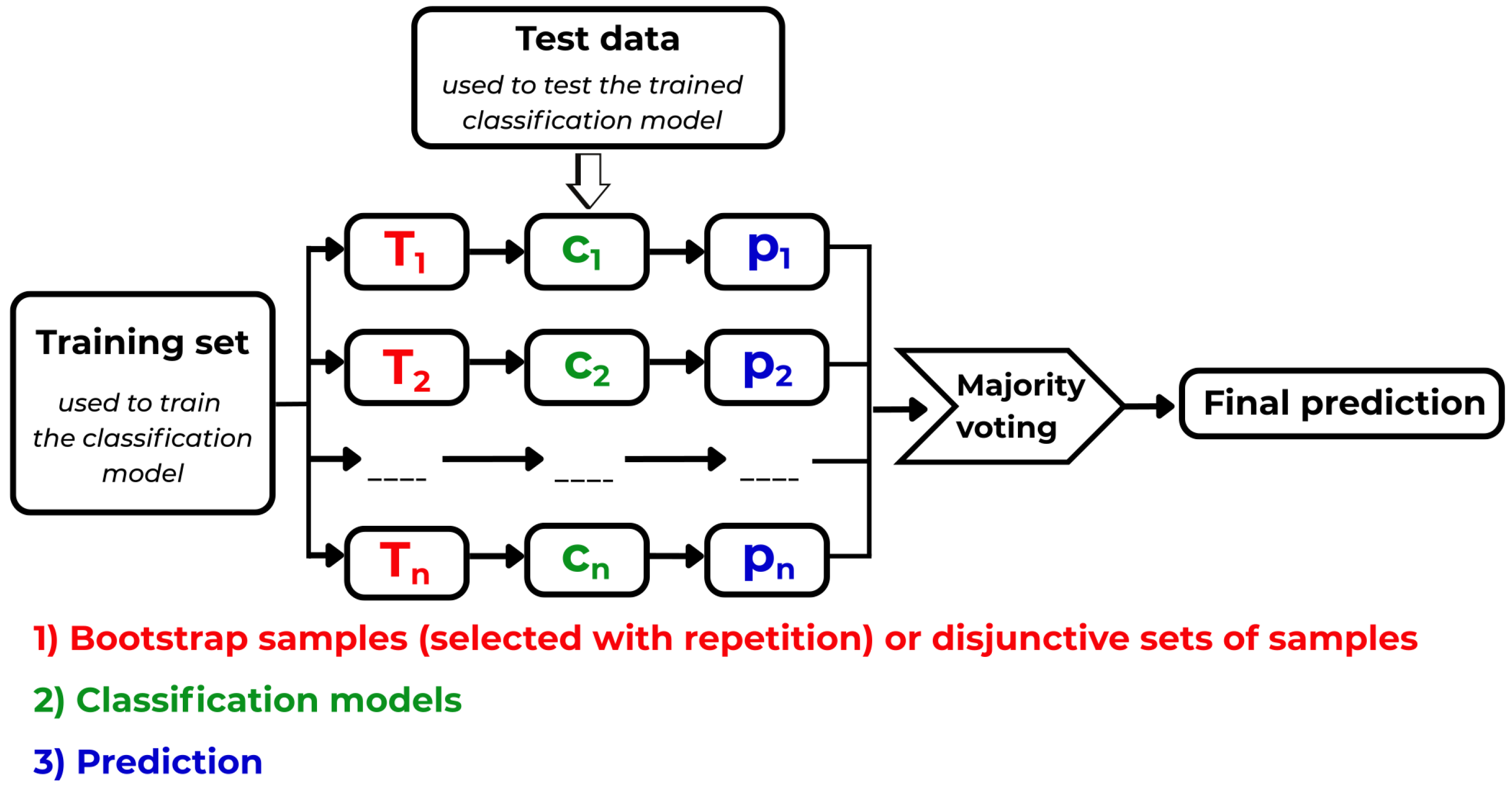
6.5.7. Random Forest (RF)
Random Forest (RF) [114,125] is a type of ensemble-based ML algorithm that employs the Bagging technique on the input data (the way of splitting the original data into subsamples). RF combines decision trees with ensemble learning using a special trick that allows overcoming the following notoriously known problem. Whenever the same training data and splitting rule are applied, a deterministic algorithm applied to construct DTs inevitably leads to the construction of the identical tree (the resulting topology of the tree is identical). This procedure does not ensure the highest possible performance of classifiers in the case of ensemble learning. Therefore, some kind of diversity is introduced to boost the RF’s performance to overcome this deadlock. Diversity is achieved during construction of RF trees by random splitting of the trees during construction process via selection of the best split using randomly chosen subset of features—simultaneously each decision tree in an RF is trained using a random subset (with repetitions) of the training data (this approach is called Bagging). The crucial moment is that random subsets of features are used for the selection of each data split—in this way, no two decision trees are identical.
The algorithm of the RF model follows this scheme:
- 1.
- Original data are split into randomly chosen subsets (bootstrapping).
- 2.
- Every decision tree is at each node selecting the best split using only a random subset of all features during its construction (this ensures diversity of trees).
- 3.
- Each constructed decision tree is evaluated for each subset.
- 4.
- The final decision is created by the majority vote of all predictions from all trees. Averaging of the values during the evaluation of the final decision is applied in regression!
6.6. Definition of ARARS Score: More Balanced Performance Measure
The performance of classifiers can be evaluated using single statistical measures such as are recall (sensitivity), specificity, ROC-AUC, and accuracy. Often, it is not sufficient. Therefore, the ARARS score was introduced (by D.B.) for more balanced evaluation of classification performance. The ARARS score is computed as an average of recall (sensitivity), specificity, ROC AUC (Receiver Operator Curve–Area Under Curve), and accuracy.
While using this score, it is much harder to report a high performance for the tested data when compared to the cases where only a single measure from the list of above-mentioned ones or some other ones is used. We are getting more robust results while using the ARARS score.
Another option, a stricter one would be to introduce the ARARS-min score (introduced by J.K.), which will take the minimal value of all statistical measures instead of the average.
this type of score was not tested in this study. It is the natural extension of the used ARARS score defined in Equation (9). Many extensions/variants of such score types can be introduced, similarly to the Equation (10).
6.7. Standardization of Features: Rescaling of Variables
Very often, the input data, which are being evaluated by ML methods, contain features that are represented at different scales, e.g., salary (1000$-45000$), size of family (1-10), and age (0-120). Such disparity of scales can cause substantial problems during evaluations by most ML methods. Without the application of data preprocessing, a feature with a wider distribution of values (e.g., salary) will dominate, and most ML algorithms (some are immune to this effect) will be unable to learn properly from the features with more compact distributions of values (e.g., family size, age) despite the fact that these features may be the most discriminating.
Therefore, in this work, features were preprocessed (standardized) by rescaling to keep the values within the same range. Mostly statistical features and their combinations together with other features were utilized in this study. All features applied in this work were standardized to zero mean and unit variance. The main reason of rescaling is that some machine learning algorithms—such as Decision Tree or Random Forest—do not depend on the feature scales and work correctly without feature rescaling; however, many other machine learning algorithms such as SVM, k-NN, logistic regression and neural networks are unable to handle features at different scales properly.
6.8. Estimates of Feature Importance: Navigation Tools Towards Viable Hypotheses
Hypothesis creation is deeply embedded within the very core of all scientific research, even when not stated explicitly. When we study a large complex system—in our case, the cardiovascular system of mammalian bodies measured by permutation entropy—using AI & ML methods, which are naturally producing many observable features; the ability to distill the most important and relevant systemic features that are capable of supporting the given hypothesis becomes one of the main differences between successful and unsuccessful research. Actually, this ability is the core of all research; only here, in ML methods, we apply it in a more explicit and naked form.
This is why the Random Forest’s useful and practical ability to distill most important features is so important—besides classification, it is often applied to estimate the importance of given features and navigate towards vital hypothesis(es). It had been repeatedly applied within this study to different feature sets to reveal the most useful ones. Keeping order in data during their evaluation is a important aspect of each ML-based study. To assist in the design of various approaches and to gain an overview of them, there are shown just four of many possible ways of data representation used in an ML study:
- (i)
- All data of one rabbit stored at one table is providing simultaneous information about all features/time and all lags L at one place (two-dimensional case, 2-D); see Figure 25. This is how data are stored in the program.
- (ii)
- Vertical viewpoint displays varying features (alternatively varying time) for a fixed, preselected lag L for each rabbit separately (3-D case), one horizontal plane represents one rabbit; see Figure 26,
- (iii)
- Horizontal viewpoint displays varying lag L against a fixed, preselected feature for each rabbit separately (3-D case), one horizontal plane represents one rabbit; see Figure 27.
- (iv)
- The PeE time-slicing method takes values from curves of different rabbits—in total N for a given fixed at the preselected time t—and create a time slice (2-D case) from them. This time slice is consecutively displayed in N-dimensional space (N-D case)—a 3D example with with the same #L of three different rabbits is shown in Figure 28.
When dealing with a single rabbit, either a horizontal or vertical point of view on data can be applied; see Figure 25 (and arrows pointing in both perpendicular directions there). This basically means that the features applied in most of the tested ML methods were divided throughout this study into two main groups with different viewpoints for easy orientation: vertical and horizontal. See the following figures for details: Figure 26 and Figure 27.
The vertical viewpoint has been applied within almost all ML methods; see Figure 26. It has been evaluated for one given, preselected lag L independently of others and encompasses important time moments, statistical features, DFT and DWT coefficients, etc. It was evaluated independently on sub-intervals (control and methoxamine) and, on the whole, non-divided curves for some specific features. It had proved itself as the most productive approach that had been found in this ML study; nevertheless, it can be different in different studies.
The horizontal viewpoint, Figure 27, is created by taking a fixed feature and by varying the value of the lag L, which represents one possible example of data and feature evaluation according to the table in Figure 25. In this case, the lag L is varying for the selected, fixed feature, which is time t (as an example, time was fixed to the value = 15). On the right side of Figure 27, data are represented in the table for a given rabbit where the line is red-circled. The plot on the left contains all tables for all rabbits simultaneously—one table, one rabbit, one horizontal plane.
The time-slicing method, see Figure 28, was used to create sequences of multidimensional points (each refers to one particular dimension/rabbit): the point is different one for each fixed time-slice t and one chosen sub-interval (either control or methoxamine). This procedure was done for all rabbits i (where ) using identical preselected lag L for each point. See the left panel of Figure 28 for a simplified description of the creation of slices from curves and the right panel for the constructed points.
As already said, a repetitive application of the time-slicing method in a sequence of multidimensional points in the space of Ls—one point for each specified time-slice—(other statistical features, e.g., mean were not used) where all these points were evaluated simultaneously; see Figure 28. Subsequently, a Random Forest was used to identify the most discriminating dimensions (values of L) based on this set of points. Unfortunately, the time-slicing method failed in the identification of useful Ls because the highest ARARS scores from used ML methods on identified Ls were unsatisfactory. Contrary to it, the vertical approach was completely successful. The feature combinations using the prefix called ’best’ indicate cases where only sets of useful values of L (identified by the time-slicing method) were used during experiments. The identified important features were verified using box plots (Box-and-Whisker plots).
7. Conclusions
The complexity of observed phenomena that are observed in medicine and biomedical research has already reached levels that are intractable by humans. This is reflected in the segmentation and specialization of medical care, where different specialists are not capable of tracking other medical specializations and disciplines. This situation is causing huge problems in research and practice as benefits and risks of therapies are becoming gradually blurred and side effects of therapies convoluted. Hence, new mathematical tools capable of describing this complexity are becoming strongly searched for. Progress depends on the development of the current mathematics, computer science, and biology that are being increasingly applied in medicine. It is the moment where complex systems, computer science, emergence, self-organization, AI, ML intersect with biomedical research.
We observe that mathematical descriptions of biological phenomena are shifting from the well-known, established statistical models and linearized models towards novel, mostly unknown, still fast-developing, nonlinear, massively parallel models—this shift is opening doors towards more realistic mathematical descriptions of complicated, intractable, complex systems that are, in general, made from large numbers of copies of relatively trivial agents that are interacting mutually in nonlinear ways and citations in them. The inevitable shift in paradigm—from sequential and mechanistic towards massively parallel and emergent one—leads to the latest, most advanced, most abstract approaches in mathematical descriptions of naturally observed phenomena, see [24,25,26,27]. We are not sure which methods prove themselves as productive and which do not. We must try them all and decide afterward. Telling a priory ’no’ can lead to missing some really novel, helpful, reliable approaches.
As we already know from statistical physics, which deals with large ensembles of simple, mutually interacting entities—e.g., gases—, entropy serves as the macroscopic measure of information content that often allow avoid a detailed, beyond-our-reach description of complex systems at the microscopic level. This feat is achieved by the use of some appropriate type of measure of system’s features, parameters, or signals. In other words, entropy allows measuring intrinsic properties of complex systems—to us, hidden, unreachable, and impossible to quantify—without studying their detailed interactions. Entropy describes systems by using some macroscopic measure of distributions of physical quantities (biosignals in medicine) instead of their direct study. Exactly this strategy was applied in this paper. The activity of a complex system—encompassing the heart, cardiovascular center, and the whole cardiovascular system, including its complete regulation—is measured using a specific type of complexity measure called permutation entropy that is suitable to quantify biosignals (in our case, ECG recordings).
In this study, due to the insufficient capability of all statistical methods to accomplish the following task, AI/ML methods were applied to distill hidden dependencies between the presence/absence of arrhythmia for a given rabbit and the shape & time evolution of permutation entropy evaluated for all ECG recordings of all animals. This task was accomplished by the automated testing of a huge number of hypotheses.
It was demonstrated that arrhythmia can be predicted using standard and advanced statistical features only using about five-minute-long control and methoxamine intervals—application of the methoxamine drug is relatively safe when compared to dofetilide—with 93% sensitivity, specificity, and ROC–AUC using SVM, RF, LR, k-NN, and EL from all tested ML techniques: all techniques gave the very same results independently. The above-given results were achieved for the comparison of normal versus TdP & non-TdP rabbits. In reality, we do not know whether non-TdP arrhythmia expressing rabbits will get a TdP or another deadly arrhythmia later in time within coming hours, days, and weeks. Hence, it is a good idea to put both arrhythmia cases into the same group.
The following was tested: Preselected moments (found by a RF) were added to the previously used sets of features while the ML techniques stayed the same. In such case, arrhythmia could be predicted with 99% probability of sensitivity, specificity, and ROC–AUC. This double selection of time moments and features seems to be a bit unrealistic, as the total number of data and features used in the paper is too low: results indicate overfitting. Large and more symmetrical data sets can show different outcomes. Additionally, when non-TdP rabbits got shifted to the group of normal rabbits (an intentionally incorrect shift), high asymmetry among input data caused overfitting towards a much larger number of normal rabbits; hence, the message is that such highly asymmetrical cases must be taken with extreme care.
It was found that TdP, VT, and VF arrhythmia can be predicted using only mild drug insults (with methoxamine) of the heart tissues and regulatory systems for about five minutes, which decreases the danger of the actual arrhythmia onset compared to the application of more severe insults (with dofetilide). The methoxamine probe provides sufficient information for prediction of arrhythmia, but it must be confirmed on larger data sets. It is demonstrated that for the onset of arrhythmia, the actual, dynamical response of each heart to abrupt changes in the heart regulatory system (kind of dip tests) is crucial. In this study, there are present only two ends of the causal chain that are existing within the physiological network: disruption of ion channels via their disruptors (methoxamine and anesthetic) on one side and the response of the heart tissue in concert with the cardiovascular center to this insult. Both are reflected within the ECG recording due to varying action potential propagation speeds. This gives us initial information that can be applied in more detailed studies of physiological axes/chains of the physiological network.
Author Contributions
Conceptualization, J.K.; methodology, J.K. and D.B.; software, J.K. and D.B.; validation, J.K. and D.B.; formal analysis, J.K.; investigation, J.K. and D.B.; resources, J.K.; data curation, J.K. and D.B.; writing—the original draft preparation (only the research part and ML methods draft), J.K. and D.B.; writing—review and editing, J.K.; visualization, J.K. and D.B.; supervision, J.K.; project administration, J.K.; funding acquisition, J.K. All authors have read and agreed to the published version of the manuscript. Details: The model was proposed, and results were achieved during the contact (2016-17), except for the ones with excluded non-TdP arrhythmia. The text was prepared independently after the end of the contract (J.K.), except for parts of the introduction, ML-results (first half), and conclusions. Classification of TdP arrhythmia vs. normal plus non-TdP rabbits (second half, counterexample) was prepared after the end of the J.K. contact (2018). This is the last publication, for which research was done and the publication written during the employment at BMC Pilsen. L. Nalos, D. Jarkovská, and M. Štengl performed all experimental measurements of ECG recordings on rabbits and are entirely responsible for their originality and consistency. The publication fee was waved by the MDPI, the publisher of the Software journal.
Funding
This study had been partially supported by the National Sustainability Program I (NPU I) Nr. LO1503 provided by the Ministry of Education, Youth, and Sports of the Czech Republic (JK). ML research was done by D.M. during preparation of his M.Sc.degree thesis (details there and above). Details are declared in the author contributions. The publication fee was waved by the journal Software, MDPI.
Data Availability Statement
Software is available at the following web pages: permutation entropy evaluation [92] www.researchgate.net/publication/392937277], ECG visualization [93] www.researchgate.net/publication/350621866 https://www.researchgate.net/publication/350621866, and statistical description of entropy and ML methods [104] www.researchgate.net/profile/Dmitryi_Bobir/394027065].
Acknowledgments
J.K. acknowledges 20 years of help and support from the leading MD of the arrhythmology department (primář) of IKEM, Prague, Jan Bitešník with compensation for severe cardiomyopathy, operations, and patient explanation of details of heart damage. This research is the result of all of his help and hence is dedicated to him along with all people of The Czech Republic. This research is dedicated to all who are currently suffering and will be suffering in the future from the heart damages that require 24/7/365 preventive monitoring of the heart condition.
Conflicts of Interest
Declare conflicts of interest or state “The authors (J.K.) declare no conflicts of interest.”
Abbreviations
The following abbreviations are used in this manuscript:
| ECG | Electrocardiogram |
| PVC | Premature ventricular contraction |
| TdP | Torsades de Pointes |
| VT | Ventricular tachycardia |
| VF | Ventricular fibrillation |
| HRV | Heart rate variability |
| CS | Complex system |
| PeE | Permutation Entropy |
| STD | Standard deviation |
| AI | Artificial Intelligence |
| ML | Machine Learning |
| SVM | Support vector machine |
| RF | Random forest |
| LR | Logistic regression |
| EL | Ensemble learning |
| DM | Data mining |
Appendix A. Used ML Methods Strategies and Specifications
Appendix A.1. Figure Depicting Strategy and Structure of All Performed ML Experiments
One of the main goals of this paper is to provide non-specialists and decision-makers an easy-to-follow methodical explanation of the way, which is enabling them to search for the best possible hypothesis that can be made above experimentally measured data (or complexity measures) using AI & ML. The process of hypothesis creation is often hidden behind the creation of every AI & ML model despite its great importance. Premature narrowing of the pool of all possible hypotheses can lead to an unwanted deadlock of the entire research. Actually, the right strategy of hypothesis creation is science at its purest, which has been practiced for millennia. AI & ML is nothing more than automation of this process.
This appendix is providing a detailed graphical description of hypothesis creation that is visually complementing Section 4.8 and Section 5.1; it enables a quick orientation within all search paths. The very same approach can be used in any scientific discipline dealing with any-signal (insert instead the word ’any’ for a signal from the field of research area under consideration and not only a ’bio’) that captures the essential features of the observed—for us incomprehensible and immeasurable—complex system under study. A CS can be biological, chemical, atmospheric, climatic, stock market, market, societal, etc.
A map of all ML methods applied to all curves, their selected parts, and/or features during the search for the best classification of arrhythmia, which are explained in details within Section 4.8, is depicted in Figure A1. Unsuccessful results are depicted in black, partially successful results in blue, and fully successful evaluations in red.
Figure A1.
A map of all ML methods that were applied in the search for hidden dependencies among curves (marked as EC–entropy curves) and arrhythmia (see Section 4.8 for detailed information about all used methods). The number of applied ML experiments is relatively high and covers a major part of standard ML algorithms. Successful, partially successful, and unsuccessful results are provided in red, blue, and black, respectively.
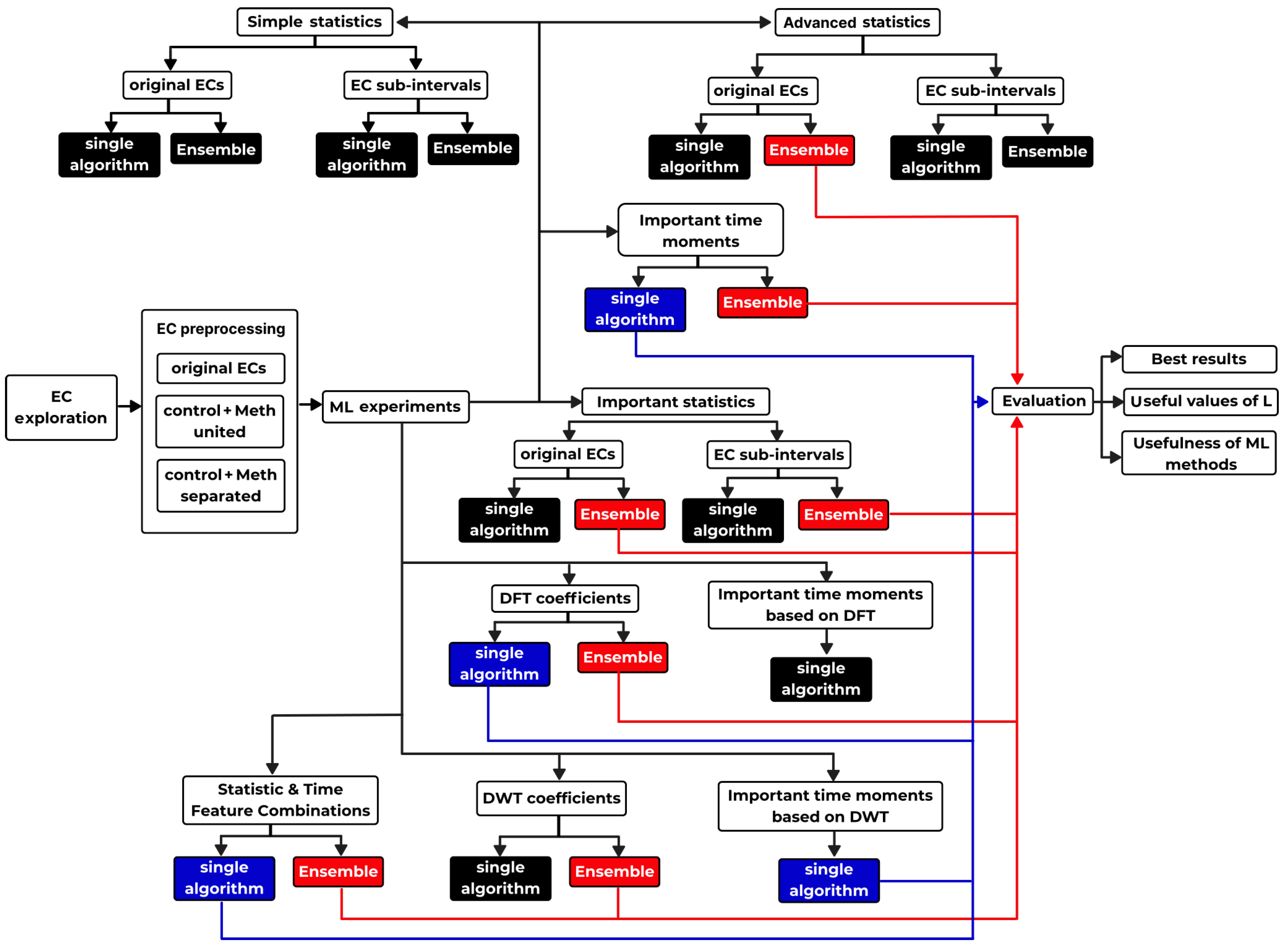
Such a graphical depictions of the search for the results can be very useful for many researchers. It helps to keep an easy overview of what was already tried and did not work well and what remains to test. Actually, this search process can be at least partially automated. In the future, such procedures will be applied to search and report novel, so far unknown data dependencies.
Appendix A.2. Principles of Ensemble Learning: Explained on SVM
The core principles of ensemble learning are demonstrated in a particular case of SVM ensemble, which is shown in two subsequent Figure A2 and Figure A3. The first Figure A2 demonstrates ensemble learning using a specific combination of evaluated s within both evaluated sub-intervals that is going to be tested for all rabbits. There is shown an ensemble method that is using a combination of one specific ensemble of SVM methods applied to both intervals (methoxamine and control) along with a number of preselected curves. Together they give much better output than any single method alone.
Figure A3 demonstrates voting done for one specific rabbit that was performed for the identical combination of data and methods as shown in Figure A2—data in the form of selected intervals from curves are fed into the ensemble of SVM classifiers. Outputs from all classifiers is shown in blue and red.
Figure A2.
The topology of the applied SVM ensemble applied to both intervals (methoxamine & control) in parallel and simultaneously to a number of preselected different curves (marked as EC–entropy curves) from all possible is depicted. Each SVM classifies different intervals and curves independently. In general, ensembles of ML methods can together ’see’ more information than any single ML method alone—they together give higher accuracy, specificity, and sensitivity of 93%. Each single method alone gives substantially lower values than the ensemble!
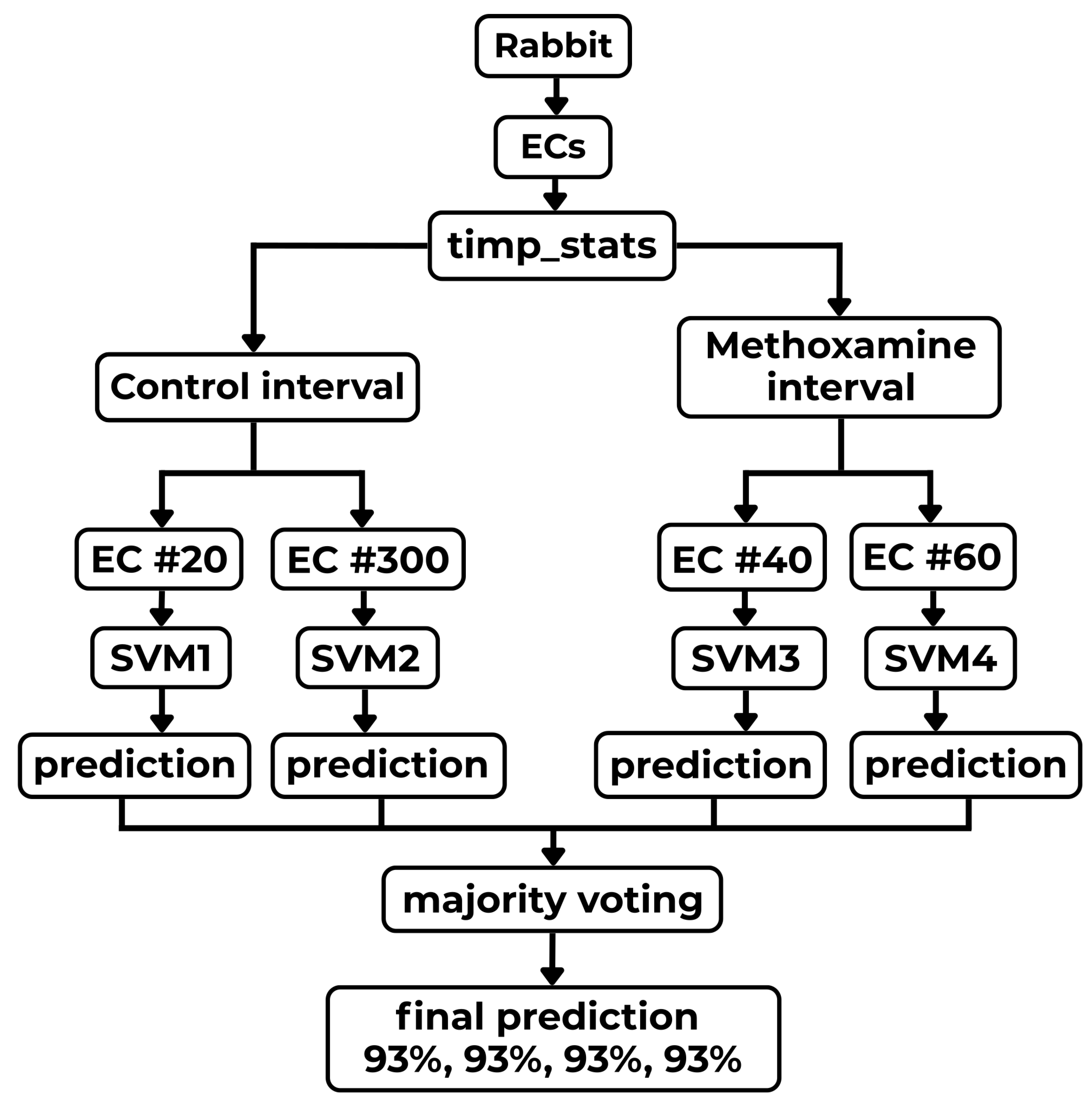
Figure A3.
This figure demonstrates one specific instance of voting where the SVM ensemble (shown in Figure A2) votes for one specific input. Its final decision for a selected rabbit is demonstrated in detail. The ensemble votes and arrives at the conclusion that arrhythmia is the winner for the given rabbit/input (combination of voting above different s (marked as EC–entropy curves) in both sub-intervals). Principally, different instances of majority voting employing other combinations/ensembles of ML algorithms are very similar to the demonstrated SVM ensemble method.
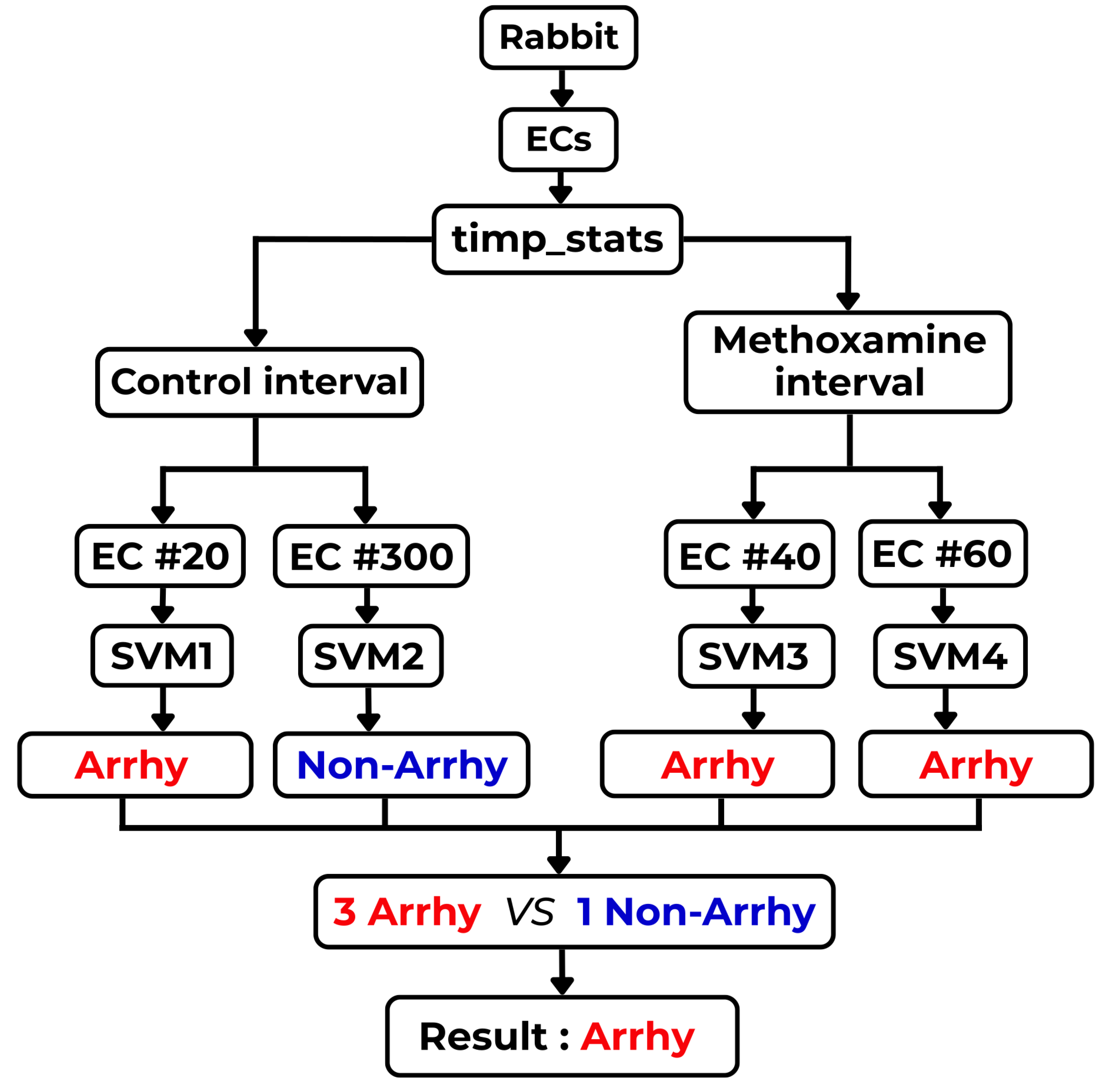
Appendix A.3. Gini Impurity
When a decision tree is designed, a basic problem immediately arises. It is necessary to make a sequence of decisions according to which criterion, feature, or value is optimal to start splitting classified values first, which should be left for later, and which goes last (as the graph leaves). What is the optimal procedure, which finds the best classification tree? This all is multiplied due to the fact that such trees can become huge. Basically, there are two ways to accomplish this task: using information entropy (as is defined in Section 3) or Gini impurity (this section). Gini impurity has one great advantage—it has much lower computational complexity due to the lack of logarithmic function in it when compared to information entropy. This will make a huge difference during construction of large decision trees.
In the case of classification trees, the Gini impurity (Gini index) measures the impurity of a node that helps to decide the one that is the best for a split
where J is the number of classes present in the node, and is the distribution of the classes in the node. Every single data split must maximize the decrease in impurity (minimize the Gini index impurity criterion).
Because it is very important to understand the core message behind the Gini Impurity , a simple two class example is provided in several variants: from A to E. Each variant explores a different mixture of those two classes.
Table A1.
Several examples, which range from A to E, of Gini impurity evaluation that can be applied to develop a decision tree are shown. The whole evaluation is demonstrated step-by-step in each table line. The cases having the lowest value of , pure cases, are the best for a split. It is logical: the best case allows 100% classification.
| Example | Class A [%] | Class B [%] | Total # samples [100 %] | Filling formula | Final |
|---|---|---|---|---|---|
| A | 100 | 0 | 100 | 0 | |
| B | 75 | 25 | 100 | ||
| C | 50 | 50 | 100 | ||
| D | 25 | 75 | 100 | ||
| E | 0 | 100 | 100 | 0 |
From Table A1, it is evident that the lowest value of Gini impurity is reached for pure cases, whereas its highest value is reached for equiprobable cases, similarly to entropy. Logically, our goal is to split two cases in such a way that they lead to the best split possible. Hence, the node with the lowest value of Gini impurity is preferred in each next step building a given decision tree!
When there are more nodes in the split, let’s say two, it is necessary to evaluate weighted average of both children (or more) that occur in the split. Firstly, Gini impurity is evaluated separately for the left and right child and , respectively. It is followed by evaluation of the weights of both children, and , and from it the final value of Gini impurity
where and . The weighting procedure mitigates the situations where one node is getting many more cases than the other one—fewer cases bring lower weight.
Appendix B. Reliability, Reproducibility, and Safety of ML/AI Solution–Critical Questions
This subsection presents selected answers to the "20 Critical Questions for Health-Related ML/AI Technology" provided in the paper [98]. Only questions relevant to this AI research, which is dealing with the predictions of arrhythmias, are answered. The paper [98] was written, and questions were created by a panel of experts who deal with the application of statistical and AI/ML methods in medicine in all phases of biomedical research and their clinical applications.
Appendix B.1. Point 1.: "How is ML/AI Model Embedded in Feedback Loops to Facilitate a Learning Health System?"
Ideally, AI applications in medicine must be open to continuous development and adaptation as methods of medical care are constantly changing. It is not a sufficient and wise practice to collect patients’ data just once, create a database, and keep it closed—for later use of such database to train and validate all future ML/AI models. Firstly, it is fundamental to leave the database as an open-access one and enable other researches to freely use it in searching for better AI/ML models and descriptions. Secondly, it is necessary to continuously update the database—by creating distinct, updated versions of it with certain periodicity and with clearly stated closing dates—and keep it always open to inserting new data whenever necessary in the future updates. This might become useful in future retrospective studies.
Continuous inserting of new data into databases can help to mitigate drift of measured data as medical therapies and drugs are constantly changing. Data measured twenty years ago can be the result of different clinical approaches and hence be obsolete today. Ideally, the databases should be renewed within short period of time or at least every several years.
In this context, wearable devices, which are continuously collecting anonymized patient data and continuously sending this data back to specialized open-source data-centers, will eventually enable a fully automated creation of medical databases used in training and assessing the quality of AI models. Updated AI/ML algorithms can be periodically upgraded on all devices. This approach will become really practical in situations such as COVID-19 infectious disease—which is experimentally treated by various medical drugs, some of which are causing TdP arrhythmia—where speed of data collection, therapy testing, and information sharing is critical for the survival of many people.
Contrary to the above proposed ideas, current medical research procedures go completely in the opposite direction. Data are collected on animal models or from patients. Unfortunately, data collection is supported by public grants, but the data themselves are kept private by data creators (researchers or groups), fragmented, unavailable to other researchers, and closed to their further development and updates. This situation is substantially impeding the development of novel, more effective AI/ML tools and their easy comparison. All the above-discussed factors blocked validation of the software proposed in this paper on human data (see below for details).
Appendix B.2. Point 2.: "What Is the Health Question Relating to Patient Benefit?"
The main goal of this research—based on complexity & ML/AI—is to answer whether it is possible to predict in ventricles originating arrhythmia (TdP, VT, and VF), which are acquired using only one lead ECG recordings, at least tens of minutes or even hours before their onset. The results achieved on a rabbit model are giving a possibility of such predictions. Purely statistical approaches commonly used in biomedical research were demonstrated to be unable to discern ECG recordings into two groups: the arrhythmia-acquiring rabbits and the resistant ones. Similar results were achieved on human ECG recordings of patients from emergency rooms [103] using a deep learning technique. Both approaches suffer from a low number of studied cases; and hence, the reliability of achieved results must be further checked (see Point Appendix B.1).
Appendix B.3. Point 3.: "When and How Should Patients Be Involved in Data Collection, Analysis, Deployment, and Use?"
Patient and public involvement (PPI) in the collection of ECG recordings can be present in all steps of the data science cycle: collecting ECG recordings, detecting an ML/AI algorithm, developing the algorithm, and applying, testing, and providing feedback on the algorithm in practice. Data collection can be built strictly around PPI; this allow a higher controlability of biomedical research. The entire process of public involvement can be stratified into several layers: preventive, checkup, and detailed examination. This will dramatically increase the effectiveness of the data acquisition and the subsequent therapy because it allows only suspicious physiological data of patients—according to predefined criteria—to be evaluated in the higher, more resource-demanding (and more expensive) data acquisition & evaluation levels.
This type of research—due to the abundance of physiological data in all layers and due to its effectiveness—can become a prototype for all future research areas in physiology and medicine as such because they are already collecting huge databases of patient physiological data that will be processed by ML/AI algorithms. In this way, the allocation of financial resources can be optimized towards greater effectiveness within medical care.
Appendix B.4. Point 4.: "Is There Organizational Transparency about the Flow of Data?"
In this computational study, data (ECGs) are the input of the evaluation. Data was provided [52,88,89] with zero transparency about data flow and interpretation by the authors of the rabbit study. Data were delivered in the form of ECG recordings (by D.J. & M.S.) with annotated moments when drug applications were initiated. Data were grouped according to the classified type of arrhythmia: normal, TdP arrhythmia, or non-TdP arrhythmia. This information create the entire input of this study. It was shortly mentioned by M.S. that intended research did not produce expected outcomes using simple statistical methods [88]. The experiments—to which used ECG recordings belongs—used a rabbit model to study the influence of a high-cholesterol diet on the incidence of medically drug-provoked arrhythmia. According to the authors M.S., D.J., and L.N., no successful correlation between level of cholesterol and arrhythmia incidence was found; no more details were shared with the authors of this complexity research. No citation of data, link to an open-source ECG recordings database, or any research based on those data was provided by the authors of the data despite several explicit requests.
Experiments on the rabbit model—and hence all ECG recordings used in this study—were carried out using financial support from the state grants provided either by the Czech Ministry of Education or by the Czech Grant Agency. Despite all of this, surprisingly, the database of the experimental data, including ECG recordings, was not publicly available as of August 2017.
In the future applications of the presented predictive AI/ML software, in general, the flow of data should become fully transparent. Due to the need of only one-lead ECG data, it would be possible to use a simple commercially available wearable devices having a chest stripe (a t-shirt- or bra-embedded electrodes) to record ECGs recorded in specific locations. Patients, sportsmen, and all who get interested in it can use it themselves. Such data can be uploaded and anonymized prior to their insertion into huge databases containing various types of heart rhythms, tachycardia, and arrhythmia. Those databases would serve as learning & test-bed places for the development of novel AI/ML based algorithms that enable an automatic recognition of various heart diseases. Anonymized data will protect patients/users from identity theft.
Data acquired by hospitals can be gathered similarly on a voluntary basis and provided to developers of the software—data are just a few mouse clicks away. In return, this methodology will enable hospitals to acquire reliable classification & predictive tools for free, which could be used in in-bed settings and allow them to operate in fully automatic regimes. The capability of such AI/ML software to predict incoming life-threatening heart events would become very important. In-hospital acquired knowledge and experiences will enable us to provide qualified feedback for the future development of more advanced software.
Appendix B.5. Point 5.: "Is the data suitable to answer the clinical question, i.e., does it capture the relevant real-world heterogeneity, and is it of sufficient detail and quality?"
In this pilot study, it was demonstrated that curves are sufficiently sensitive to capture subtle changes of the heart’s operational mode—that is, all under the assumption that data are measured correctly and provided in their original, unchanged, measured form [52,88,89]. TdP, VT, and VF arrhythmia are associated with a substantial decrease in complexity that is clearly expressed on curves. Additionally, it was shown that AI/ML methods are sensitive in the prediction of incoming heart arrhythmia—originating in the ventricles (this location is important in this study as we do not know how it will work in atria-located arrhythmia)—up to one hour before their actual onset using only a few minutes of ECG recordings. Even the best-trained cardiologists are unable to accomplish such predictions due to huge distribution of data and their subtleties in time and space.
It was observed on curves and using ML-results that changes preceding the initiation of TdPs are sufficiently pronounced just a few minutes after the onset of methoxamine infusion; there is not a necessity to apply a much greater insult to the heart by applying dofetilide infusions. This is a very favorable situation, as patients’ lives are not put at great risk while using a milder type of medically induced increase of the heart rate and heart electrophysiology disruption (methoxamine). We can speak about a chemical probe; see Section 6.4, in the case of in-this-way induced insults. In the case of naturally occurring TdP or VT arrhythmia—due to cardiomyopathy or heart infarction—the changing electrical properties of the ventricular tissue(s) become the ’probe’ on its own.
The impact of decreasing sampling rate from 1000 Hz down to 500 Hz, 200 Hz, and even 100 Hz was tested. The curves were resistant to such dramatic decreases of the sampling rate and still managed to maintain the same profile of curves. Subsequent testing of the influence of such decrease on results produced by AI/ML methods is difficult & time-consuming and hence, it was not performed.
It is necessary to rule out a possibility that other types of arrhythmia or ECGs’ changes generated during physical & mental loads, stress, under medications, or hormonal imbalances can lead to similar patterns of entropy development, and hence, TdPs and VTs can get mis-classified. Ruling out this possible failure of the AI/ML method is solvable only when large databases of all possible arrhythmia and ECG changes are available and the given method is tested against all of them—such misclassified cases will affect (decrease) the overall value of the method’s specificity (see Point Appendix B.1).
One of the authors J.K. contacted two hospitals in the Czech Republic in order to acquire full, one-hour-long ECG recording periods prior arrhythmia onset. Human ECG recordings of TdP arrhythmia from ICU units are lying just a few mouse clicks away. Both hospitals declined. The management of the Biomedical Center in Pilsen (BCP), including M.S., had been discouraging those requests for human ECGs made by J.K.. Later, all contacts to other hospitals and research centers in the country and abroad was repeatedly and explicitly forbidden by the management of BCP—the reason was that “It is not a priority of BCP”. Hence, no testing on human ECGs was performed, to the surprise of J.K., despite the readiness of the software since spring 2017. That’s all despite the fact that soon after finalizing this study (Aug 2017)—by preparing the draft of the results part—the first real applications of AI/ML methods in the detection of arrhythmia occurred in wearable devices, e.g., Apple Watch [21]. Hence, the demand from industry is huge.
Appendix B.6. Point 6.: "Does the validation methodology reflect the real world constrains and operational procedures associated with data collection and storage?"
A database of ECG recordings [52] was created using the rabbit model. It will not be regularly updated. Nevertheless, the model can get reevaluated in the future when new medical drugs start to be used.
The mission creating a public, open-access database of human ECG recordings proposed by J.K. was not accomplished due to not being the priority of the institution. Recently, the availability of human data acquired from wearable devices (ECG recording chest straps [126], specialized personal ECG recorders, and smartphones/watches [21,105,127,128,129,130]) is exponentially increasing, which creates a new potentially usable pool of ECG recordings. This gives hope that nonprofit organizations can collect and gradually create free, open-access, validated, and tested ECG databases in this way. All AI researchers and wearable device software developers will definitely appreciate this effort.
Generally speaking, any developed algorithm based on AI/ML methods that is using a permanently frozen database can sooner or later become obsolete as new methods, procedures, treatments, and medical drugs start to be applied/used in medicine. Therefore, a methodology performing periodic reevaluation and retesting of the newest versions of databases against all AI/ML algorithms is desirable—fortunately, it can be fully automated. Such permanent testing and resetting of the methodology and testing validity can be done even locally at each hospital separately—it will enable the detection of any deviation from the previous effectiveness of AI/ML methods quickly.
Appendix B.7. Point 7.: "On what basis are data accessible to other researchers?"
As of August 2017, input data—in the form of ECG recordings [52]—were not openly accessible to other researchers. It would be of great usefulness to create a publicly available database of TdP arrhythmia using the university IT infrastructure. Additionally, it was proposed to make the software and all research data on prediction of TdP arrhythmia openly accessible to anyone because it can help promote research and save a lot of lives (the software can be found here [92,104]). A boom of wearable devices [21,126,127], which could substantially benefit from open research on TdP arrhythmia, occurred just a few years later! Additionally, we have the COVID-19 infection that is often treated by hydroxy-/chloroquine, causing TdPs; software of this type can substantially improve medical care in such cases.
States should reconsider allocation of their scarce grant resources to research groups that are monopolizing the public resources for the promotion of their own work and position against needs and well-being of the whole populations—all by state sponsored research must be made open-source by default. This strategy will avoid repetition of the same research in every country separately and simultaneously allow mathematicians and AI researchers to push research driven by those data fast-forward.
Appendix B.8. Point 8.: "What computational software resources are available, and are they sufficient to tackle this problem?"
No commercial software—including MatLab—was available to predict arrhythmia from ECG recordings during this research. This led to the necessity of a gradual development of the own software tools (LINUX BASH and Gnuplot scripts, C++ program) and later the use of freeware (Python ML methods). The software evaluating permutation entropy was originally written in C++ (now rewritten in Python [92]): its input is an ECG and the output is the set of evaluated entropy curves with different lags of this ECG. Various combinations of evaluated entropy having different lags L for the same ECG recording, heart rate, and HRV were grouped together and inserted in the same figures—it served as a first-level analysis of arrhythmia predictions. Figures were created using the BASH shell script that is calling the graph-creating program Gnuplot in LINUX (see the software package [92,104] for details (ML methods here [90])); it is a flexible and fast way of enabling the production of thousands of figures in a very short time using a prepared batch file that repeatedly calls the shell program, creating each plot according to provided parameters (the name of the given input ECG recording and a lag L value).
During research, the entire procedure going from evaluation of entropy to creation of various combinations of figures depicting arbitrary combinations of evaluated entropy, HR, and HRV curves, was fully automated using batch files calling said C++ programs and BASH scripts. Manual evaluations are possible too.
The complexity analysis was subsequently followed by the evaluation of various data: simple statistics, heart rate, heart rate variability, etc. using simple BATCH scripts. This approach to the problem analysis—using various statistical methods—was explicitly requested as a standard procedure used in medical research. As expected, none of the selected statistics proved the capability of discriminating between arrhythmogenic and non-arrhythmogenic rabbits (see Figure 15 and Figure 16).
This was the moment when many AI/ML methods were applied to entropy data. Initially, the use of simple and advanced statistical methods were systematically tested on entropy curves without any effect; see Section 4.5 and Figs. Figure 16 and Figure 15 there. This confirmed the correctness of the decision, J.K., to carry out fully AI-/ML-methods-based research using curves. In the preparatory step, many features were defined that were tested by a wide range of different AI/ML methods; see Section 4.7. This led to results presented in this paper.
Whether this approach is suitable to predict TdP arrhythmia from ECG recordings or not must be further explored and evaluated on many databases of human ECG recordings. Such databases should contain five- to ten-minute-long periods of time before the onset of TdPs. ECG recordings can be taken at least hours and, if possible, days, weeks, or even months before and right after their onset, or alternatively ECGs of patients weeks or months before the onset of TdPs and after their onset. Five-minute-long one-lead ECG recordings are sufficient according to our observations. This is a challenging task for various reasons but definitely worth trying (research groups creating such databases will gain many citations).
The following developed programs—entropy evaluation (Python program for permutation entropy evaluation), data visualization (BASH shell scripts plotting figures using Gnuplot), Python ECG visualization program [93], and AI/ML computational resources (Python programs applying standard AI/ML methods involved in Python’s SciPy library)—are open-access and freely available on ResearchGate [92,104]. Development of ML methods is documented in [90].
Appendix B.9. Point 9.: "Are the reported performance metrics relevant for the clinical context in which the model will be used?"
There are very few existing studies dealing with the prediction of VTs or TdPs from ECG recordings in the literature. One study predicting VTs using an AI deep learning technique from a set of ECG recordings of ER patients [103] has reported specificity and sensitivity of 89%. The current study has a specificity & sensitivity of 93% on the rabbit model [52]. Therefore, the current study is interesting for clinical use, and it should be tested on human ECG recordings. A comparison of the current study and the AI deep learning study [103] above a carefully selected, identical database of ECG recordings is desirable. Nevertheless, this comparison requires freely available software, which is available only for the present study using entropy and ML methods [92,104] and not for the deep learning study [103].
Performance of the proposed AI/ML method can be tested on human ECG recordings—exactly in the same way as in this study—using a batch file that accomplishes the whole AI/ML evaluation process fully automatically. The only necessary step from the user of the program is to create a batch file with links to the sources of raw ECG data (this can be automated too). The classification successes of the AI/ML prediction algorithm above a large collection of ECG recordings are stored. Later, the specificity & sensitivity of the whole batch re-evaluated whenever new ECG is added. AI/ML methods are not fully automated in the software package [92,104].
Reported sensitivity and specificity of TdP arrhythmia prediction would be interesting to the clinical use—higher mean values greater importance of the reported arrhythmia danger—as it would enable employees of ER, ICU, and other highly specialized units to prepare for incoming life-threatening events in patients.
This AI/ML algorithm is very suitable to be used in all in-hospital and even out-of-hospital settings when a potentially lethal TdP arrhythmia-generating drug is administered to a patient. This software, when it gets embedded in a wearable device, is capable of reporting incoming TdP events in a fully automatic mode. Additionally, it can connect itself to the healthcare provider using the Internet within tens of minutes or even hours before an arrhythmia occurs.
Appendix B.10. Point 10.: "Is the reported gain in statistical performance with the AI/ML algorithm clinically justified in the context of any trade-offs?"
We have very few, if any, algorithms capable of predicting arrhythmia in clinical use. Use of such an algorithm can become a great enabler in specialized clinical units (ER, ICU, etc.) and especially in out-of-clinic settings when endangered patients leave the hospital and stay at home, or are going to work. With the increasing capabilities and preciseness of both entropy measures and AI/ML arrhythmia-predicting algorithms, we can cover population segments of people who might benefit from such an approach.
It is easily imaginable that a patient, sportsman, fireman, bus driver, pilot, military personnel, etc. can be equipped with an ECG recording chest stripe or intelligent underwear that will be either gathering data for further evaluation or directly sending them into a wearable device/mobile device that will immediately report the actual state of the heart. It can revolutionize medical care and enable its decentralization, and, simultaneously, it can introduce individualized approaches to every patient.
A very important aspect of this approach is the possibility to build huge, reliable databases of arrhythmias, including periods of time that is preceding them by hours, days, months, and even years. This would become a gold mine for development of all future AI/ML methods predicting arrhythmia.
Appendix B.11. Point 11.: "Is the ML/AI algorithm compared to the current best technology, and against other appropriate baselines?"
The developed algorithm could not be compared to the best technology directly for the following reasons. Firstly, the clinical practice does not use unsupervised algorithms, which are predicting an incoming arrhythmia, due to a lack of reliable algorithms. Secondly, the only known similar algorithm predicting VTs from ECG recordings of ER patients [103] is based on a deep learning algorithm—where neither the database of ECG recordings of arrhythmia nor the algorithm itself is publicly available. Deep learning algorithms are having several drawbacks: a) there is necessity of applying huge computing power to train them, and b) their interpretation is impossible for almost all neuronal networks.
Comparison of the proposed algorithm and the deep learning algorithm [103] can be done only indirectly via their specificity and sensitivity: both are equal to 93% for the current algorithm and both are equal to 89% for the deep learning algorithm. Authors of this study are prepared to compare this method [92,104] with other methods above sufficiently large database(s) of animal and human arrhythmia (TdP, VT, and VF).
It is worth of mentioning one class of algorithms that are applied in modern implantable cardioverter-defibrillators (ICDs). Because charging of a capacitor for a prospective defibrillating discharge takes many seconds, each defibrillator has an active a short-term (about one minute), arrhythmia detection/prediction algorithm, usually based on a complexity measure. It detects a substantial change of entropy measure that initiates charging of the capacitor. Another, more precise algorithm makes the final decision using longer data on whether the discharge will be delivered or not. The proposed algorithm is consistent with already used algorithms.
Appendix B.12. Point 12.: "Are different parts of the prediction modeling pipeline available to others to allow for method reproducibility, including: statistical code for ’preprocessing’, and the modeling work-flow (including the methods, parameters, random seeds, etc. utilized)?"
The entire set of software tools, which was used to evaluate this pilot study, is fully and freely available as an open-source code on ResearchGate [92,104]. The database of ECG recordings of rabbits acquiring Torsades de Pointes arrhythmia and those resistant to it [52] used to train AI/ML methods is not open-source; all who would like to use it must ask the authors of that research [52], who created and administer those data. Availability of open-source ECG recordings will be valuable for many researchers who want to establish themselves in the research field and will definitely increase the overall quality and credibility of this research area; see Point Appendix B.7 for more information.
Appendix B.13. Point 13.: "Are the results reproducible in settings beyond where the system was developed (i.e., external validity)?"
An improved algorithm—after adjustments and reevaluation—can be easily used for prediction of TdP, VT, and probably even VF arrhythmia because the principle of the creation of the algorithm remains the same. Changes leading to the occurrence of TdP arrhythmia, which are reflected by a decrease in measured permutation entropy, are gradual and can be observed at least tens of minutes or even an hour before their onset. For the VTs, it could be similar. VFs were detected in some rabbits, they occurred after the onset of a TdP arrhythmia. They were associated with decreased entropy too. TdP, VT, and VF are indistinguishable from entropy curves.
It is very easy to use one’s own ECG recordings and study them with this software, because all parts of the used software are open source [92,104]. External validity can be tested without any problems just by filling batch scripts using the correct names of files storing raw data of ECG recordings (which can be stored anywhere on the system) in the format: <implicit line number> <potential> with a space in between those two numbers.
Appendix B.14. Point 14.: "What evidence is there that the model does not create or exacerbate inequities in health-care by age, sex, ethnicity or other protected ethnicities?"
This feature of the model was not yet tested due to a small set of used data. Nevertheless, one important experimental observation occurred: older rabbits typically got arrhythmia, whereas younger ones did not [88]. It was confirmed theoretically, as can be seen from observed entropy curves, that most of the young rabbits were easily capable of compensating for all drug-induced insults to the heart’s electrophysiology, and their entropy curves stayed at a more or less same level. It was not the case for most of the older rabbits [88].
It this study, it is important to have as low false negative cases as possible because they are leading to death. The main goal of this software is to not miss any approaching arrhythmia. The specificity of ML algorithms was detected at the level of 93%.
Appendix B.15. Point 15.: "What evidence is there that clinicians and patients find the model and its output (reasonably) interpretable?"
From the user’s point of view, the proposed AI/ML model predicting TdP arrhythmia is very similar to the well-known Apple Watch 4 feature that enables the detection of atrial fibrillation (AFib) [21,105,110], which represents a known example of biosignal classification. This software can gain popularity among Apple Watch and other device users. Predicting arrhythmias is more difficult than their mere classification. Therefore, issues related to the interpretation of clinic and out-of-clinic use are quite similar to Apple Watch 4 AFib detection.
A big advantage of the proposed AI/ML model is that it is partially a white box contrary to deep learning models, which are full black boxes—there are no tools capable of decoding decisions made by DL models. The white part of the box in the proposed & ML algorithm/model comes from the fact that entropy curves enable an easy visual inspection of their actual changes, and hence, easy anticipation of a possibility of incoming arrhythmia—this part is very useful to MDs and even to patients to understand! Only the part of the proposed AI/ML model, which directly uses AI methods, is a part of a black box.
Hence, there is a possibility, which will very probably be appreciated by patients, that the algorithm can feed data into a visualization application, giving a complex visual response. This might be welcoming for some patients, as they will be more incorporated in the detection of arrhythmia and can relate their daily routines to changes observed on evaluated entropy curves and displayed by a wearable device. It might become a psychological advantage of the white-box part of the algorithm. As a bonus, an easier interpretability of entropy curves can provide some valuable insights—not know now at the moment of research—to medical professionals. Additionally, patients can participate in the improvement of the algorithm by recording and sending critical phases of their ECG recordings.
Appendix B.16. Point 16.: "What evidence is there of real world model effectiveness in the proposed clinical setting and how are unintended consequences prevented?"
The author, J.K., attempted to acquire anonymized ECG recordings of patients who acquired TdP arrhythmia recorded during their in-hospital stays; see the Point Appendix B.6, because without those data, it was impossible to study the effectiveness of the proposed AI/ML algorithm in real settings.
The proposed AI/ML algorithm can be, in general, tested in several contexts, which when done properly, can substantially enhance its specificity and sensitivity. Actually, large-scale applications of the algorithm can improve all parameters of the method. Those different contexts of the AI/ML algorithm application are: intensive care units & resuscitation units, common hospital rooms, sportsmen, recreational sportsmen, drivers & pilots & others who can cause big damage when they acquire heart arrhythmia, and people using wearable devices. All this can dramatically enlarge databases of stored arrhythmia cases and hence, benefits` from it.
Appendix B.17. Point 17.: "How is the model being regularly re-assessed, and updated as data quality and clinical praxes changes (i.e., post-license monitoring)?"
This was addressed by a proposal to design, build, update, and maintain the open-source database providing ECG recordings of TdP arrhythmia events; see the Point Appendix B.12 for details. Everyone can test and calibrate any software against such database. It is the best and the most transparent way of developing of software that has high public interest, as it can save many lives (not only now, since spring 2020, during ongoing worldwide pandemics of COVID-19). A constant competition among different algorithms can be implemented in this way. Results are, in such cases, directly comparable by everyone.
Appendix B.18. Point 18.: "Is the ML/AI model cost-effective to build, implement, and maintain?"
It is easy and cheap to build and implement this AI/ML algorithm. The most costly is building the TdP arrhythmia database, which requires a huge number of annotated ECG recordings. The database should be maintained, regularly updated, and follow the actual development of the medical care. Development of the software that is implementing the algorithm depends on the updates of the database. Updating of the AI/ML algorithm can be done in fully automatic mode with only visual checkups by an expert. Once developed, the software is cheap.
Software implementing AI/ML algorithms can be used by people & patients in out-of-the-hospital settings in their daily lives by having wearable devices. This, when accompanied by collecting interesting recordings from the patients’ wearable devices, in fully automatic mode, can help to build a huge database of all types of heart arrhythmia and tachycardia, which in turn will speed up the development of algorithms capable to classify and predict those events. The biggest obstacle to the use of this approach will be the anonymization of the acquired patients’ data.
Regularly updated, unsupervised ML techniques should be periodically executed using such databases. It can help to uncover either hidden, yet undiscovered dependencies or novel ones after adding new data.
Appendix B.19. Point 19.: "How will potential financial benefits be distributed if the ML/AI model is commercialized?"
The algorithm was jointly developed by J.K. using state grant money support and by D.B. as a part of a master’s thesis project (no support). The main author J.K. decided that this paper and accompanying software will be provided for free under the GPL-v3 license—in its basic live-saving versions—to anyone who is developing life-saving algorithms predicting incoming life-threatening arrhythmia. Future, advanced versions of the software that will be developed later—for drivers, pilots, and other socially important occupation, together with sportsmen and high-end customers—can be commercialized under the terms of the GPL-v3 license [92,104].
Data necessary for the development of this software can be collected in publicly available open-source databases of physician-annotated arrhythmia, which will be collected by hospitals using money from states or health insurance companies. Collecting those data will be voluntary.
Appendix B.20. Point 20.: "How have the regulatory requirements for accreditation/approval been addressed?"
Not addressed yet.
Appendix C. Results–Part 2: An Example of Falsified Machine Learning Results for Normal and Non-TdP Against TdP Acquiring Groups of Rabbits
This section was designed by J.K. to be identical with the results presented in Section 4.9—where normal rabbits are compared against the group of both TdP & non-TdP rabbits—with the following changes: (i) non-TdP arrhythmia are excluded from arrhythmias group and shifted to Normal group, (ii) eight batches are used (instead of the original ten) in ensemble learning techniques (later manually changed by D.B. because too few curves for TdP arrhythmia is present), (iii) more L values is involved in the ensemble learning techniques (decision were made automatically by methods).
Due to a miscommunication and misunderstanding of J.K.& D.B., the following changes were made instead of the planned ones. All changes are the same as above except that half of the TdP rabbits were excluded and non-TdP rabbits were erroneously shifted to the group of normal rabbits, which does not make sense as arrhythmia-resistant rabbits get mixed with those susceptible. Hence, this section compares half of TdP with Normal and non-TdP rabbits. This is not correct, but J.K. decided to keep this section in the paper in order to demonstrate where deliberate manipulations with experimental data can lead to. Please note an alarming fact associated with those results: they are looking too good to be trustworthy.
The narrowing of the pool of classified curves to TdP (arrhythmogenic) and Normal (non-arrhythmogenic) rabbits inevitably led to less available data. In this case, there were 23 non-arrhythmogenic rabbits and only 9 arrhythmogenic ones. Taking into account those facts, it was necessary to decrease the number of cross-validation folds from 10 to 8. The results were expected to be overfitted as there was an insufficient amount of data with their huge asymmetry.
Results were achieved by the application of the ensemble approach. In which a combination of 3 to 32 (identical or different) ML algorithms (see column ’Used Algorithms’) that were applied to preselected features (see column ’Features’) and extracted from the original curves for two different intervals (control and methoxamine); see Table A2. The final prediction is accomplished by the majority vote among the given ensemble.
As can be seen from the Table A2 and Table A4, many L values were used in predictions. Almost each value of L achieved an ARARS score greater than 80% (see Table A4). However, in many cases, sensitivity was approximately 50% and specificity was approximately 95%. Thus, the results indicate extreme overfitting on non-arrhythmogenic s.
Appendix C.1. Normal and Non-TdP Against TdP Acquiring Rabbits: Lags L of PeE That Are Giving Best Results for Listed Combinations of Features and Algorithms
This table (identical to Table 6 from the Section 4.9.1) contains information about the used values of the L parameter that complements the table above. The values of the L parameter in this table are those with an ARARS score of at least 75% for the appropriate machine learning algorithm.
Table A2.
The table provides an overview of the best results (with ARARS score > 75%) achieved for combinations of features and ML algorithms sorted according to features, used methods, and lags L for control and methoxamine groups in the case of Normal and non-TdP versus TdP rabbits.
Table A2.
The table provides an overview of the best results (with ARARS score > 75%) achieved for combinations of features and ML algorithms sorted according to features, used methods, and lags L for control and methoxamine groups in the case of Normal and non-TdP versus TdP rabbits.
| Features | Used algorithms | Used L | |
|---|---|---|---|
| Control | Methoxamine | ||
| ISI_Top5-TM | SVM | 1, 10, 100, 20, 30, 300, 400, 50, 60, 80 |
1, 10, 20, 200, 30, 300, 5, 50, 500, 60, 70, 80, 90 |
| RF | 10, 30, 60, 70 | 10, 30, 5, 70 | |
| k-NN | 10, 20, 200, 30, 300, 400, 5, 50, 70, 80 |
20, 200, 30, 5, 90 | |
| LR | 10, 50, 60 | 70, 80, 90 | |
|
OC_Top5-ASF |
SVM | 1, 10, 100, 20, 200, 30, 300, 40, 400, 5, 50, 500, 60, 70, 80, 90 |
|
| SVM, RF, k-NN, LR |
RF: 1, 10, 100, 200, 30, 300, 40, 400, 5, 50, 500, 60, 70, 80, 90 LR: 10, 100, 20, 30, 40, 5, 50, 60, 80, 90 k-NN: 1, 10, 100, 20, 200, 30, 300, 40, 400, 5, 50, 500, 60, 70, 80, 90 SVM: 1, 10, 100, 20, 200, 30, 300, 40, 400, 5, 50, 500, 60, 70, 80, 90 |
||
| OC_ASF | SVM | 10, 100, 20, 30, 300, 40, 5, 50, 70, 80, 90 | |
| ISI_Top5-ASF | SVM | 20, 30, 300, 60, 70 | 10, 100, 40, 5, 500 |
| ISI_Top5-TM & ISI_Top5-ASF | SVM, RF, k-NN, LR |
RF: 10, 20, 300, 60 LR: 10, 300, 400, 50, 60, 80 k-NN: 20, 300, 5, 60 SVM: 10, 100, 20, 30, 300, 400, 5, 50, 60, 80 |
RF: 10, 5, 70 LR: 100, 300, 50, 500, 70, 80, 90 k-NN: 10, 100, 200, 5, 500, 70, 90 SVM: 10, 100, 200, 30, 300, 5, 50, 500, 60, 70, 80 |
| ISI-DFT_Top5-C | SVM | 10, 20, 30, 300, 40, 50, 60, 80, 90 | 100, 20, 40, 5, 70, 80, 90 |
| ISI-DWT_Top10-C | SVM | 1, 20, 60 | 1, 20, 30, 500 |
Appendix C.2. Normal and non-TdP Against TdP Acquiring Rabbits: Predictions Employing Majority Voting above Simultaneous Combinations of Classifiers for All Values of Lags L
Table A3 (identical to Table 7 from the Section 4.9.2) overviews an ensemble approach that used a combination of ML algorithms and all available information (i.e., s from different drug intervals and of different values of the L parameter) in order to make the final prediction by majority voting. Importantly, each algorithm used only those values of the L parameter that achieved an ARARS score of at least 75% for the appropriate algorithm. The Table A3 lists results where the process map IDs provide the navigation keys to the items in Section 4.7.3. The values of the L parameter, which were used for prediction, are listed in the Table A2.
Table A3.
Results were achieved by the application of the ensemble approach, where a combination of 3 to 32 (identical or different) ML algorithms (column ’Used Algorithms’) applied to preselected features (column ’Features’) originating in the curves for two different intervals (control and methoxamine) in the case of TdP versus Normal and non-TdP rabbits. The final prediction is done by the majority voting among the given ensemble. Only classifiers (ML methods) with ARARS > 75% were used in ensemble learning. Abbreviations are Se, Sp, AUC, and Acc stand for sensitivity, specificity, ROC area under curve, and accuracy. Process map ID provides the navigation key in Section 4.7.3. Arrows show changes of values when compared to those present in Table 7.
| Features | Process map ID | Used algorithms | Se (%) | Sp (%) | AUC | Acc (%) |
|---|---|---|---|---|---|---|
| ISI_Top5-TM | aii4 | SVM | 1.0 | 1.0 | 1.0 | 1.0 |
| RF | 0.65 ↓ | 1.0 ↑ | 0.82 ↓ | 0.9 ↓ | ||
| k-NN | 0.77 ↓ | 1.0 | 0.88 ↓ | 0.93 ↓ | ||
| LR | 0.71 ↓ | 1.0 ↑ | 0.85 ↓ | 0.92 ↓ | ||
| OC_Top5-ASF | di2d | SVM | 0.77 ↓ | 0.95 ↓ | 0.86 ↓ | 0.9 ↑ |
| SVM, RF, k-NN, LR | 0.69 ↓ | 0.99 | 0.84 ↓ | 0.91 ↑ | ||
| OC_ASF | ci2d | SVM | 0.72 ↓ | 0.96 ↑ | 0.84 | 0.89 ↑ |
| ISI_Top5-ASF | dii2d | SVM | 0.88 ↓ | 0.98 ↑ | 0.93 | 0.95 ↑ |
| ISI_Top5-TM & ISI_Top5-ASF | eii4 | SVM, RF, k-NN, LR | 0.99 ↓ | 1.0 | 0.99 ↓ | 0.99 ↓ |
| ISI-DFT_Top5-C | fii | SVM | 0.99 | 1.0 ↑ | 0.99 | 0.99 |
| ISI-DWT_Top10-C | hii | SVM | 0.98 ↑ | 1.0 ↑ | 0.99 ↑ | 0.99 ↑ |
Results from the table clearly indicate overfitting to normal curves, as there is a majority of them present in the input data: arrows present in the Table A3 clearly indicate this fact.
Appendix C.3. Normal and non-TdP Against TdP Acquiring Rabbits: List of Best ML-results for All Values of Lags L—Guide to Easy Orientation
This section (same procedure as in Section 4.9.3; see Table 8 there for comparison) contains a summary (see Table A4 below) of the most useful values of the L parameter with ARARS scores greater than 80% in the case of TdP and Normal rabbits. When values of the L parameter with the ARARS score are greater than 90%, their values are explicitly displayed. As can be seen from the table, the most useful values of the L parameter are 10, 50, 60, 70, 80, 100, 300, and 500.
Table A4.
The list of the most useful values of the lag L parameter with an ARARS score of at least 80% (symbol ’x’) in the case of TdP and Normal rabbits. All ARARS values greater than 90% are provided with their actual numerical values.
Table A4.
The list of the most useful values of the lag L parameter with an ARARS score of at least 80% (symbol ’x’) in the case of TdP and Normal rabbits. All ARARS values greater than 90% are provided with their actual numerical values.
| L | ||||||||||||||||
|---|---|---|---|---|---|---|---|---|---|---|---|---|---|---|---|---|
| 1 | 5 | 10 | 20 | 30 | 40 | 50 | 60 | 70 | 80 | 90 | 100 | 200 | 300 | 400 | 500 | |
| RF | x | x | x | x | x | x | x | x | x | x | x | x | x | x | ||
| SVM | x | x | x | x | x | x | 0.93 | x | x | 0.91 | x | x | x | 0.91 | x | 0.92 |
| k-NN | x | x | 0.91 | x | x | x | x | x | x | 0.91 | x | 0.91 | x | x | x | x |
| LR | x | x | x | x | x | x | x | x | x | x | x | x | x | x | ||
| Ensemble | x | x | x | x | x | x | x | 0.94 | 0.91 | x | x | x | x | x | x | x |
The reason to provide tables displaying the most useful values of lag L is to provide the visual clue of which measures are measuring and predicting arrhythmia most efficiently.
References
- Van Noord, C.; Eijgelsheim, M.; Stricker, Bruno, H.Ch. Drug- and non-drug-associated QT interval prolongation. British Journal of Clinical Pharmacology 2010, 70, 16–23. [CrossRef]
- Jayasinghe, R.; Kovoor, P. Drugs and the QTc interval. Australian Prescriber 2002, 25, 63–65. [Google Scholar] [CrossRef]
- Chorin, E.; Dai, M.; Shulman, E.; Wadhwani, L.; Bar Cohen, R.; Barbhaiya, C.; Aizer, A.; Holmes, D.; Bernstein, S.; Soinelli, M.; et al. The QT Interval in Patients with SARS-CoV-2 Infection Treated with Hydroxychloroquine/Azithromycin. medRxiv 2020. [Google Scholar] [CrossRef]
- Li, M.; Ramos, L.G. Drug-Induced QT Prolongation And Torsades de Pointes. Pharmacy and Therapeutics: a peer-reviewed journal for formulary management 2017, 42, 473–477. [Google Scholar]
- Yap, Y.G.; Camm, A.J. Drug induced QT prolongation and torsades de pointes. Heart 2003, 89, 1363–1372. [Google Scholar] [CrossRef]
- Trinkley, K.E.; Page II, R.L.; Lien, H.; Yamanouye, K.; Tisdale, J.E. QT interval prolongation and the risk of torsades de pointes: essentials for clinicians. Current Medical Research and Opinion 2013, 29, 1719–1726. [Google Scholar] [CrossRef]
- Katz, A.M. Physiology of the heart, 5 ed.; Lippincott Williams & Wilkins, 2011; p. 576.
- Topol, E. Deep Medicine: How Artificial Intelligence Can Make Healthcare Human Again, 1st ed.; Basic Books, Inc.: USA, 2019. [Google Scholar]
- Cleophas, T.J.; Zwinderman, A.H. Machine Learning in Medicine - a Complete Overview; Springer, 2015; p. 516. [CrossRef]
- Kreibig, S.D. Autonomic nervous system activity in emotion: A review. Biological Psychology 2010, 84, 394–421, The biopsychology of emotion: Current theoretical and empirical perspectives. [Google Scholar] [CrossRef]
- Mauss, I.B.; Robinson, M.D. Measures of emotion: A review. Cognition and Emotion 2009, 23, 209–237. [Google Scholar] [CrossRef] [PubMed]
- Kléber, A.G.; Rudy, Y. Basic Mechanisms of Cardiac Impulse Propagation and Associated Arrhythmias. Physiological Reviews 2004, 84, 431–488. [Google Scholar] [CrossRef] [PubMed]
- Richman, J.S.; Moorman, J.R. Physiological time-series analysis using approximate entropy and sample entropy. American Journal of Physiology: Heart and Circulatory Physiology 2000, 278, H2039–H2049. [Google Scholar] [CrossRef] [PubMed]
- Costa, M.; Peng, C.K.; Goldberger, A.L.; Hausdorff, J.M. Multiscale entropy analysis of human gait dynamics. Physica A 2003, 330, 53–60. [Google Scholar] [CrossRef] [PubMed]
- Humeau-Heurtier, A. The Multiscale Entropy Algorithm and Its Variants: A Review. Entropy 2015, 17, 3110–3123. [Google Scholar] [CrossRef]
- Liang, Z.; Wang, Y.; Sun, X.; Li, D.; Voss, L.J.; Sleigh, J.W.; Hagihira, S.; Li, X. EEG entropy measures in anesthesia. Frontiers in Computational Neuroscience 2015, 9, 16. [Google Scholar] [CrossRef] [PubMed]
- Olofsen, E.; Sleigh, J.W.; Dahan, A. Permutation entropy of the electroencephalogram: a measure of anaesthetic drug effect. British Journal of Anaesthesia 2008, 101, 810–821. [Google Scholar] [CrossRef]
- Shivaram, S.; Muthyala, A.; Meghji, Z.Z.; Karki, S.; Arunachalam, S.P. Multiscale Entropy Technique Discriminates Single Lead ECG’s With Normal Sinus Rhythm and Sleep Apnea. In Proceedings of the Frontiers in Biomedical Devices, 04 2018, Vol. DMD2018-6948, p. V001T01A016. [CrossRef]
- Lee, C.H.; Sun, T.L.; Jiang, B.C.; Choi, V.H. Using Wearable Accelerometers in a Community Service Context to Categorize Falling Behavior. Entropy 2016, 18. [Google Scholar] [CrossRef]
- Vargas, B.; Cuesta-Frau, D.; Ruiz-Esteban, R.; Cirugeda-Roldan, E.; Varela, M. What Can Biosignal Entropy Tell Us About Health and Disease? Applications in Some Clinical Fields. Nonlinear Dynamics Psychology and Life Sciences 2015, 19, 419–436. [Google Scholar]
- Lynch, K. Apple Watch 4. Smartwatch, Apple Inc., Cupertino, CA, USA, 2019.
- Schulz, S.; Adochiei, F.C.; Edu, I.R.; Schroeder, R.; Costin, H.; Bär, K.J.; Voss, A. Cardiovascular and cardiorespiratory coupling analyses: a review. Philosophical Transactions of the Royal Society A: Mathematical, Physical and Engineering Sciences 2013, 371, 20120191. [Google Scholar] [CrossRef]
- Frank, B.; Pompe, B.; Schneider, U.; Hoyer, D. Permutation entropy improves fetal behavioural state classification based on heart rate analysis from biomagnetic recordings in near term fetuses. Medical & Biological Engineering & Computing 2006, 44, 179–87. [Google Scholar] [CrossRef]
- Kroc, J. Emergent Information Processing: Observations, Experiments, and Future Directions. Software 2024, 3, 81–106. [Google Scholar] [CrossRef]
- Kroc, J. Difference Between AI and Biological Intelligence Observed by Lenses of Emergent Information Processing. In Complex Systems With Artificial Intelligence; López-Ruiz, R., Ed.; IntechOpen: Rijeka, 2024; chapter 4. [CrossRef]
- Kroc, J. Exploring Emergence: Video-Database of Emergents Found in Advanced Cellular Automaton ’Game of Life’ Using GoL-N24 Software. https://www.researchgate.net/publication/373806519, 2023. Accessed as on 09-10-2023.
- Kroc, J. Robust massive parallel information processing environments in biology and medicine: case study. Journal of Problems of Information Society 2022, 13, 12–22. [Google Scholar] [CrossRef]
- Dehmer, M.; Mowshowitz, A. A history of graph entropy measures. Information Sciences 2011, 1, 57–78. [Google Scholar] [CrossRef]
- Borda, M. Fundamentals in Information Theory and Coding, 1 ed.; Springer, Berlin, Heidelberg, 2011. [CrossRef]
- Arndt, C. Information Measures: Information and its Description in Science and Engineering; Springer, Berlin, Heidelberg, 2001. [CrossRef]
- Ben-Naim, A. Entropy Demystified: The Second Law Reduced To Plain Common Sense, revised ed.; World Scientific, 2008. [CrossRef]
- Ben-Naim, A. A Farewell to Entropy: Statistical Thermodynamics Based on Information; World Scientific, 2008. [CrossRef]
- Perkiömäki, J.S.; Mäkikallio, T.H.; Huikuri, H.V. Fractal and Complexity Measures of Heart Rate Variability. Clinical and Experimental Hypertension 2005, 27, 149–158. [Google Scholar] [CrossRef] [PubMed]
- Pincus, S.M.; Gladstone, I.M.; Ehrenkranz, R.A. A regularity statistic for medical data analysis. Journal of Clinical Monitoring 1991, 7, 335–45. [Google Scholar] [CrossRef]
- Rolnick, D.; Donti, P.L.; Kaack, L.H.; Kochanski, K.; Lacoste, A.; Sankaran, K.; Ross, A.S.; Milojevic-Dupont, N.; Jaques, N.; Waldman-Brown, A.; et al. Tackling Climate Change with Machine Learning. CoRR 2019, abs/1906.05433, [1906.05433].
- Ben-Naim, A. Information, Entropy, Life and the Universe: What We Know and What We Do Not Know; World Scientific, 2015; [https://www.worldscientific.com/doi/pdf/10.1142/9479]. [CrossRef]
- Borowska, M. Entropy-Based Algorithms in the Analysis of Biomedical Signals. Studies in Logic, Grammar and Rhetoric 2015, 43, 21–32. [Google Scholar] [CrossRef]
- Pincus, S.M. Approximate Entropy as a Measure of System Complexity. Proceedings of the National Academy of Sciences of the United States of America 1991, 88, 2297–2301. [Google Scholar] [CrossRef]
- Pincus, S.M. Approximate entropy (ApEn) as a complexity measure. Chaos: An Interdisciplinary Journal of Nonlinear Science 1995, 5, 110–117. [Google Scholar] [CrossRef]
- Riedl, M.; Müller, A.; Wessel, N. Practical considerations of permutation entropy. The European Physical Journal Special Topics 2013, 222, 249–262. [Google Scholar] [CrossRef]
- Costa, M.; Goldberger, A.L.; Peng, C.K. Multiscale entropy of biological signals. Physical review. E, Statistical, nonlinear, and soft matter physics 2005, 71, 021906. [Google Scholar] [CrossRef] [PubMed]
- Costa, M.; Goldberger, A.L.; Peng, C.K. Multiscale Entropy Analysis of Complex Physiologic Time Series. Physical Review Letters 2002, 89, 068102. [Google Scholar] [CrossRef] [PubMed]
- Gao, J.; Hu, J.; Tung, W.W. Entropy measures for biological signal analyses. Nonlinear Dynamics 2012, 68, 431–444. [Google Scholar] [CrossRef]
- Bari, V.; Girardengo, G.; Marchi, A.; De Maria, B.; Brink, P.A.; Crotti, L.; Schwartz, P.J.; Porta, A. A Refined Multiscale Self-Entropy Approach for the Assessment of Cardiac Control Complexity: Application to Long QT Syndrome Type 1 Patients. Entropy 2015, 17, 7768–7785. [Google Scholar] [CrossRef]
- Shannon, C.E.; Weaver, W. The Mathematical Theory of Communication; Urbana: University of Illinois Press, 1998. [Google Scholar]
- Shannon, C.E. A mathematical theory of communication. The Bell System Technical Journal 1948, 27, 379–423. [Google Scholar] [CrossRef]
- Guido, S.; Müller, A.C. Introduction to Machine Learning with Python; O’Reilly Media, 2016.
- Mitchell, T.M. Machine Learning; McGraw-Hill Series in Computer Science, McGraw-Hill Education, 1997.
- Hastie, T.; Tibshirani, R.; Friedman, J. The Elements Of Statistical Learning: Data Mining, Inference, and Prediction, 2 ed.; Springer Series in Statistics, Springer, New York, 2009.
- Shalev-Shwartz, S.; Ben-David, S. Understanding Machine Learning: From Theory to Algorithms; Cambridge University Press, 2014. [CrossRef]
- Hastie, T.; Tibshirani, R.; Friedman, J.; Franklin, J. The Elements of Statistical Learning: Data Mining, Inference, and Prediction. The Mathematical Intelligencer 2004, 27, 83–85. [Google Scholar] [CrossRef]
- Jarkovská, D.; Nalos, L.; Štengl, M. ECG reccordings of methoxamine and dofetilide induced Torsades de Pointes arrhythmias on rabbit model having fat-rich diet. Technical report, Charles University, Faculty of Medicine in Pilsen, Department of Physiology, 2013-2014.
- Yuan, Q.; Zhou, W.; Li, S.; Cai, D. Epileptic EEG classification based on extreme learning machine and nonlinear features. Epilepsy Research 2011, 96, 29–38. [Google Scholar] [CrossRef] [PubMed]
- Carricarte Naranjo, C.; Sanchez-Rodriguez, L.M.; Brown, M.M.; Estévez, B.M.; Machado, G.A. Permutation entropy analysis of heart rate variability for the assessment of cardiovascular autonomic neuropathy in type 1 diabetes mellitus. Computers in Biology and Medicine 2017, 86, 90–97. [Google Scholar] [CrossRef] [PubMed]
- Ravelo-Garcia, A.G.; Navarro-Mesa, J.L.; Casanova-Blancas, U.; Martin-González, S.; Quintana-Morales, P.; Guerra-Moreno, I.; Canino-Rodrígues, J.M.; Hernández-Pérez, E. Application of the Permutation Entropy over the Heart Rate Variability for the Improvement of Electrocardiogram-based Sleep Breathing Pause Detection. Entropy 2015, 17, 914–927. [Google Scholar] [CrossRef]
- Bandt, C.; Pompe, B. Permutation Entropy: A Natural Complexity Measure for Time Series. Physical Review Letters 2002, 88, 174102. [Google Scholar] [CrossRef]
- Zanin, M.; Zunino, L.; Rosso, O.A.; Papo, D. Permutation Entropy and Its Main Biomedical and Econophysics Applications: A Review. Entropy 2012, 14, 1553–1577. [Google Scholar] [CrossRef]
- Bian, C.; Qin, C.; Ma, Q.D.Y.; Shen, Q. Modified permutation-entropy analysis of heartbeat dynamics. Physical review. E, Statistical, nonlinear, and soft matter physics 2012, 85, 021906. [Google Scholar] [CrossRef]
- Malik, M.; Camm, A.J. Heart rate variability. Clinical Cardiology 1990, 13, 570–576, [https://onlinelibrary.wiley.com/doi/pdf/10.1002/clc.4960130811]. [Google Scholar] [CrossRef]
- Camm, A.J.; Malik, M.; Bigger, J.T.; Breithardt, G.; Cerutti, S.; Cohen, R.J.; Coumel, P.; Fallen, E.L.; Kennedy, H.L.; Kleiger, R.E.; et al. Heart Rate Variability: Standards of Measurement, Physiological Interpretation, and Clinical Use. Task Force of the European Society of Cardiology the North American Society of Pacing Electrophysiology. Circulation 1996, 93, 1043–1065. [Google Scholar] [CrossRef]
- Acharya, U.R.; Joseph, K.P.; Kannathal, N.; Min C., C.; Suri, J.S. Heart Rate Variability. In Advances in Cardiac Signal Processing; Acharya, U.R.; Suri, J.S.; Spaan, J.; S.M., K., Eds.; Springer, Berlin, Heidelberg, 2007; pp. 121–165. [CrossRef]
- Bravi, A.; Longtin, A.; Seely, A.J. Review and classification of variability analysis techniques with clinical applications. Biomedical Engineering OnLine 2011, 10, article. [Google Scholar] [CrossRef]
- Kroc, J.; Balihar, K.; Matějovič, M. Complex Systems and Their Use in Medicine: Concepts, Methods, and Bio-Medical applications. preprint 2019, pp. 1–21. [CrossRef]
- Zheng, R.; Yamabe, S.; Nakano, K.; Suda, Y. Biosignal Analysis to Assess Mental Stress in Automatic Driving of Trucks: Palmar Perspiration and Masseter Electromyography. Sensors (Basel) 2015, 15, 5136–5150. [Google Scholar] [CrossRef]
- Singh, R.R.; Conjeti, S.; Banerjee, R. Bio-signal based on-road stress monitoring for automotive drivers. In Proceedings of the 2012 National Conference on Communications, NCC 2012, 02 2012, pp. 1–5. [CrossRef]
- Singh, M.; Bin Queyam, A. Stress Detection in Automobile Drivers using Physiological Parameters: A Review. International Journal of Electronics Engineering 2013, 5, 1–5. [Google Scholar]
- Studer, L.; Paglino, V.; Gandini, P.; Stelitano, A.; Triboli, U.; Gallo, F.; Andreoni, G. Analysis of the Relationship between Road Accidents and Psychophysical State of Drivers through Wearable Devices. Applied Sciences 2018, 8, 1230. [Google Scholar] [CrossRef]
- Kroc, J. COMPLEX SYSTEMS AND THEIR USE IN BIOMEDICAL RESEARCH: MATHEMATICAL CONCEPTS OF SELF-ORGANIZATION AND EMERGENCE. International Congress of Cell Biology, Poster - P097, 2016. [CrossRef]
- Boltzmann, L. Vorlesungen über Gastheorie, vol. I., 1 ed.; J.A. Barth, Leipzig, 1896.
- Boltzmann, L. Vorlesungen über Gastheorie, vol. II., 1 ed.; J.A. Barth, Leipzig, 1898.
- Jaynes, E.T. Gibbs vs Boltzmann Entropies. American Journal of Physics 1965, 33, 391–398. [Google Scholar] [CrossRef]
- Poincaré, H. The Three-Body Problem and the Equations of Dynamics: Poincaré’s Foundational Work on Dynamical Systems Theory; Vol. 443, Astrophysics and Space Science Library, Springer, 2017; p. 248. [CrossRef]
- Arnold, V.I. Geometrical methods in the Theory of Ordinary Differential Equations, 2 ed.; Grundlehren Der Mathematischen Wissenschaften, Springer, New York, 2012; p. 351.
- Layek, G.C. An Introduction to Dynamical Systems and Chaos; Springer India, 2015; p. 622. [CrossRef]
- Mandelbrot, B.B. The fractal geometry of nature; W. H. Freeman & Co.: San Francisco, CA, 1982; p. 468. [Google Scholar]
- Urdan, T.C. Statistics in Plain English, 4 ed.; Routledge, 2015; p. 266.
- Kroc, J. Biological Applications of Emergent Information Processing: Fast, Long-Range Synchronization. preprint (2025), https://www.researchgate.net/profile/Jiri-Kroc/388328720.
- Russell, S.J.; Norvig, P. Artificial Intelligence: A Modern Approach; Prentice Hall series in artificial intelligence, Prentice Hall, 2010; p. 1132.
- Styer, D. Entropy as Disorder: History of a Misconception. The Physics Teacher 2019, 57, 454–458. [Google Scholar] [CrossRef]
- Clausius, R. Ueber verschiedene für die Anwendung bequeme Formen der Hauptgleichungen der mechanischen Wärmetheorie. Annalen der Physik 1865, 125, 353–400. [Google Scholar] [CrossRef]
- Clausius, R. The Mechanical Theory of Heat – with its Applications to the Steam Engine and to Physical Properties of Bodies. London: John van Voorst 1867. Retrieved 19 June 2012.
- Clausius, R. On a Mechanical Theorem Applicable to Heat. Philosophical Magazine 1870, 40, 122–27. [Google Scholar] [CrossRef]
- Boltzmann, L. Über die Mechanische Bedeutung des Zweiten Hauptsatzes der Wärmetheorie (vorgelegt in der Sitzung am 8 February 1866). k. k. Hof- und Staatsdrukerei 1866, pp. 1–26.
- Clayton. CO2. JAChS 1932.
- Bashkirov, A.G. Renyi entropy as a statistical entropy for complex systems. Theor. Math. Phys. 2006, 149, 1559–1573. [Google Scholar] [CrossRef]
- Haken, H. Information and Self-Organization: A Macroscopic Approach to Complex Systems (Springer Series in Synergetics); Springer-Verlag: Berlin, Heidelberg, 2006. [Google Scholar]
- Nicolis, J.S. Dynamics of Hierarchical Systems: An Evolutionary Approach; Springer-Verlag: Berlin, Heidelberg, 1986. [Google Scholar]
- Štengl, M. Private communications, Charles University, Faculty of Medicine in Pilsen, Department of Physiology, 2016-2017.
- Jarkovská, D. Private communications, Charles University, Faculty of Medicine in Pilsen, Department of Physiology, 2016-2017.
- Bobir, D. Identification of Pre-Arrhythmogenic Features in ECG and Other Data Using Machine Learning. Master’s thesis, Czech Technical University in Prague, Faculty of Information Technology, 2017.
- ECG Learning Center. ecg.utah.edu.
- Kroc, J. Open-source software predicting Torsade de Pointes arrhythmias, ventricular tachycardias, and ventricular fibrillations from ECG recordings: Part I—Permutation Enropy (Python and BASH). Software, GPLv3, Independent Reseach, Pilsen, The Czech Republic, 2025. [avaiable at www.researchgate.net/publication/392937277].
- Kroc, J. Visualization of ECG recordings using Python program ECG-pyview. Software, GPLv3, Complex Systems Research, Pilsen, The Czech Republic, 2020. [avaiable at www.researchgate.net/publication/350621866.
- Kroc, J. Mini-visualization program of ECG recordings: import text file and export segments of ECG. Software, GPLv3, Complex Systems Research, Pilsen, The Czech Republic, 2025. [avaiable at www.researchgate.net/publication/394454735.
- Kumar, A. HYPOTHESIS TESTING IN MEDICAL RESEARCH: A KEY STATISTICAL APPLICATION. Journal of Universal College of Medical Sciences 2016, 3, 53–56. [Google Scholar] [CrossRef]
- Amrhein, V.; Greenland, S.; McShane, B. Scientists rise up against statistical significance. Nature 2019, 567, 305–307. [Google Scholar] [CrossRef]
- Ioannidis, J.P.A. Why Most Published Research Findings Are False. PLoS Medicine 2005, 2, e124. [Google Scholar] [CrossRef] [PubMed]
- Vollmer, S.; Mateen, B.A.; Bohner, G.; Király, F.J.; Ghani, R.; Jonsson, P.; Cumbers, S.; Jonas, A.; McAllister, K.S.L.; Myles, P.; et al. Machine learning and AI research for Patient Benefit: 20 Critical Questions on Transparency, Replicability, Ethics and Effectiveness. BMJ: British Medical Journal 2020, 368, l6927. [Google Scholar] [CrossRef]
- Chalmers, A.F. What Is This Thing Called Science?, 4 ed.; Hackett Publishing, 2013; p. 304.
- Barabási, A.L.; Oltvai, Z.N. Network biology: understanding the cell’s functional organization. Nature Reviews Genetics 2004, 5, 101–113. [Google Scholar] [CrossRef]
- Barabási, A.L.; Gulbahce, N.; Loscalzo, J. Network medicine: a network-based approach to human disease. Nature Reviews Genetics 2011, 12, 56–68. [Google Scholar] [CrossRef]
- Loscalzo, J.; Barabási, A.L.; Silverman, E.K. Network medicine: Complex Systems in Human Disease and Therapeutics; Harvard University Press: London, 2017; p. 448. [Google Scholar] [CrossRef]
- Lee, H.; Shin, S.Y.; Seo, M.; Nam, G.B.; Joo, S. Prediction of Ventricular Tachycardia One Hour before Occurrence Using Artificial Neural Networks. Scientific Reports 2016, 6, 32390. [Google Scholar] [CrossRef]
- Bobir, D. Software predicting Torsade de Pointes arrhythmias, ventricular tachycardias, and ventricular fibrillations from permutation entropy; Part II—Machine Learnig (based on Python). Software, GPLv3, Czech Technical University, Faculty of Information Technologies, Prague, The Czech Republic, 2017. [avaiable at www.researchgate.net/profile/Dmitryi_Bobir/394027065].
- Perez, M.V.; Mahaffey, K.W.; Hedlin, H.; Rumsfed, J.S.; et al..; for the Apple Heart Study Investigators. Large-Scale Assessment of a Smartwatch to Identify Atrial Fibrillation. The New England Journal of Medicine 2019, 381, 1909–1917. [CrossRef]
- Lee, U.; Blain-Moraes, S.; Mashour, G.A. Assessing levels of consciousness with symbolic analysis. Philosophical Transactions of Royal Society A, Mathematical, physical, and engineering sciences 2015, 373, 20140117. [Google Scholar] [CrossRef]
- Singh, S.; Bansal, S.; Kumar, G.; Gupta, I.; Thakur, J.R. Entropy as an Indicator to Measure Depth of Anaesthesia for Laryngeal Mask Airway (LMA) Insertion during Sevoflurane and Propofol Anaesthesia. Journal of Clinical and Diagnostic Research 2017, 11, UC01–UC03. [Google Scholar] [CrossRef]
- Acharya, U.R.; Fujita, H.; Sudarshan, V.K.; Bhat, S.; Koh, J.E.W. Application of entropies for automated diagnosis of epilepsy using EEG signals: A review. Knowledge-Based Systems 2015, 88, 85–96. [Google Scholar] [CrossRef]
- Studholme, C.; Hill, D.L.G.; Hawkes, D.J. An overlap invariant entropy measure of 3D medical image alignment. Pattern Recognition 1999, 32, 71–86. [Google Scholar] [CrossRef]
- Zhou, X.; Ding, H.; Wu, W.; Zhang, Y. A Real-Time Atrial Fibrillation Detection Algorithm Based on the Instantaneous State of Heart Rate. PLoS ONE 2015, 10, e0136544. [Google Scholar] [CrossRef]
- Breiman, L. Statistical Modeling: The Two Cultures (with comments and a rejoinder by the author). Statist. Sci. 2001, 16, 199–231. [Google Scholar] [CrossRef]
- Panik, M. Regression Modeling: Methods, Theory, and Computation with SAS; CRC Press, 2009.
- Breiman, L.; Friedman, J.H.; Olshen, R.A.; Stone, C.J. Classification and Regression Trees; Wadsworth International Group: Belmont, CA, 1984. [Google Scholar]
- Breiman, L. Random Forests. Machine Learning 2001, 45, 5–32. [Google Scholar] [CrossRef]
- Friedman, J.H. Greedy Function Approximation: A Gradient Boosting Machine. Annals of Statistics 2000, 29, 1189–1232. [Google Scholar] [CrossRef]
- Rumelhart, D.E.; Hinton, G.E.; Williams, R.J. Learning Representations by Back-propagating Errors. Nature 1986, 323, 533–536. [Google Scholar] [CrossRef]
- Cortes, C.; Vapnik, V. Support-Vector Networks. In Proceedings of the Machine Learning; 1995; pp. 273–297. [Google Scholar] [CrossRef]
- Friedman, N.; Geiger, D.; Goldszmidt, M. Bayesian Network Classifiers. Machine Learning 1997, 29, 131–163. [Google Scholar] [CrossRef]
- Seeger, M. GAUSSIAN PROCESSES FOR MACHINE LEARNING. International Journal of Neural Systems 2004, 14, 69–106. [Google Scholar] [CrossRef] [PubMed]
- Hartigan, J.; Wong, M. Algorithm AS 136: A K-means clustering algorithm. Applied Statistics 1979, pp. 100–108. [CrossRef]
- Verhulst, P. Recherches mathématiques sur la loi dáccroissement de la population; Académie Royale, 1845.
- Cover, T.M.; Hart, P.E. Nearest neighbor pattern classification. IEEE Trans. Inf. Theory 1967, 13, 21–27. [Google Scholar] [CrossRef]
- Dietterich, T.G. Ensemble Methods in Machine Learning. In Proceedings of the Multiple Classifier Systems: First International Workshop, MCS 2000, Lecture Notes in Computer Science. Springer, Berlin, Heidelberg, 01 2000, Vol. 1857, pp. 1–15. [CrossRef]
- Sagi, O.; Rokach, L. Ensemble learning: A survey. WIREs Data Mining and Knowledge Discovery 2018, 8, e1249. [Google Scholar] [CrossRef]
- Ho, T. Random decision forests. In Proceedings of the Proceedings of 3rd International Conference on Document Analysis and Recognition, Los Alamitos, CA, USA, aug 1995; Vol. 1, p. 278. [CrossRef]
- Polar developers. Polar H 10 Heart Rate Sensor. ECG recording, Polar Electro Oy, Kempele, Finland, 2018.
- Samsung developers. Samsung Galaxy Watch S4. Smartwatch, Samsung Electronics Co., Ltd., Seoul, South Korea, 2019.
- Periyaswamy, T.; Balasubramanian, M. Ambulatory cardiac bio-signals: From mirage to clinical reality through a decade of progress. International Journal of Medical Informatics 2019, 130, 103928. [Google Scholar] [CrossRef] [PubMed]
- Léger, L.; Gojanovic, B.; Sekarski, N.; Meijboom, E.J.; Mivelaz, Y. The Impending Dilemma of Electrocardiogram Screening in Athletic Children. Pediatric Cardiology 2016, 37, 1–13. [Google Scholar] [CrossRef] [PubMed]
- Giebel, G.D.; Gissel, C. Accuracy of mHealth Devices for Atrial Fibrillation Screening: Systematic Review. JMIR mHealth and uHealth 2019, 7, e13641. [Google Scholar] [CrossRef]
Figure 1.
Independent throws of three dice: Only ten possible outcomes/microstates from all 216 possible are shown. (A) All dice give the identical output simultaneously. It leads to six possible outcomes; one of them is 111. (B) Two dice give identical outcomes, and one die gives a different output; an example is given by three different combinations of dice (2, 6, 6). (C) All three dices give different outcomes; different combinations of dice (1, 3, 5) are shown. Please note the fact that the B contains all cases of A, and the C contains all cases of A and B.
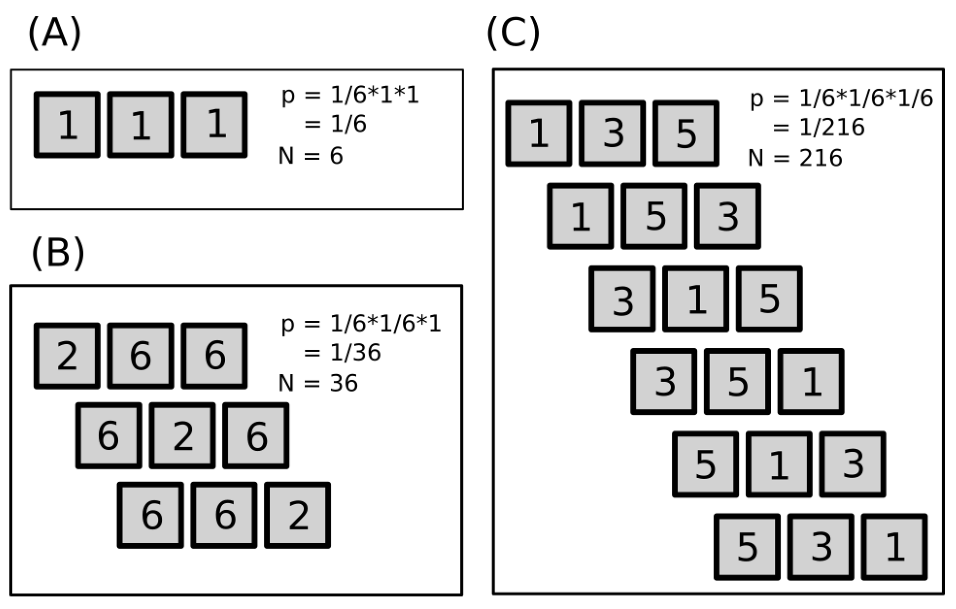
Figure 2.
The change of distributions of the #-of-microstates for all possible throws giving the same normalized sum with respect to the macrostates (dice throw sums), which was performed for 3, 4, 5, 6, 7, 8, 9, and 10 dice, is shown. The 10 dice curve is the most inner one. Values are relative and enable an easy visual inspection: the #-of-microstates is divided by the total #-of-all-microstates, and the sum is divided by the maximal sum for a given number of dice. The qualitative convergence of the distribution towards the normalized value of the sum that is around 0.5 is obvious. For an extra-large number of dice, the distribution becomes a narrow peak located around 0.5 .
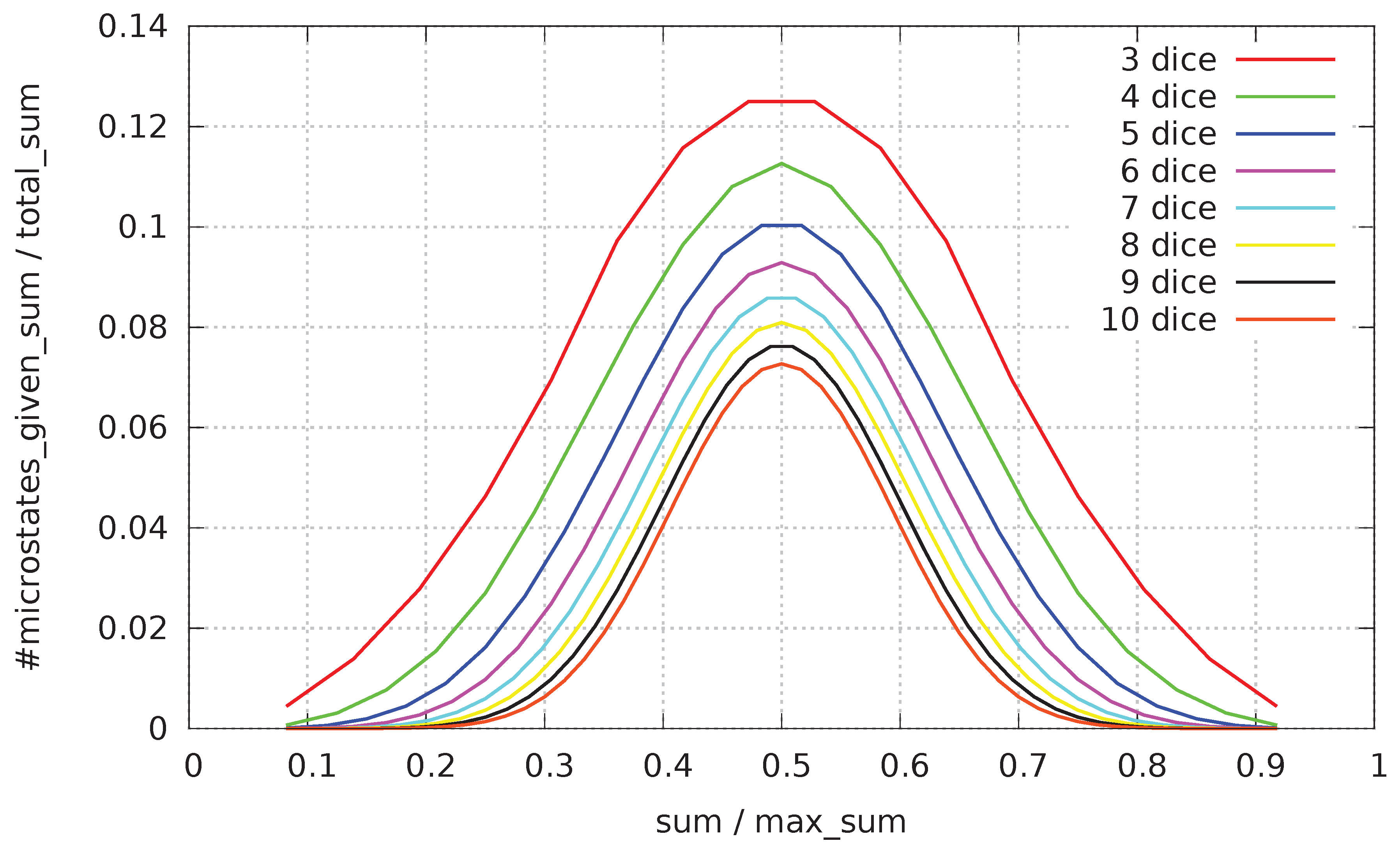
Figure 3.
Particles are moving in eight directions: (A) Only one possible direction of particle movement is allowed (direction depicted by the arrow), in the trivial case where all particles move in the same way (the average speed of the group is maximal and equal to the speed of each particle). (B) Eight different directions of particle movement: particles can move in any direction with probability . (C) In one random configuration of eight-directional movement of particles, the average speed of particles is close to zero (the group speed is low).
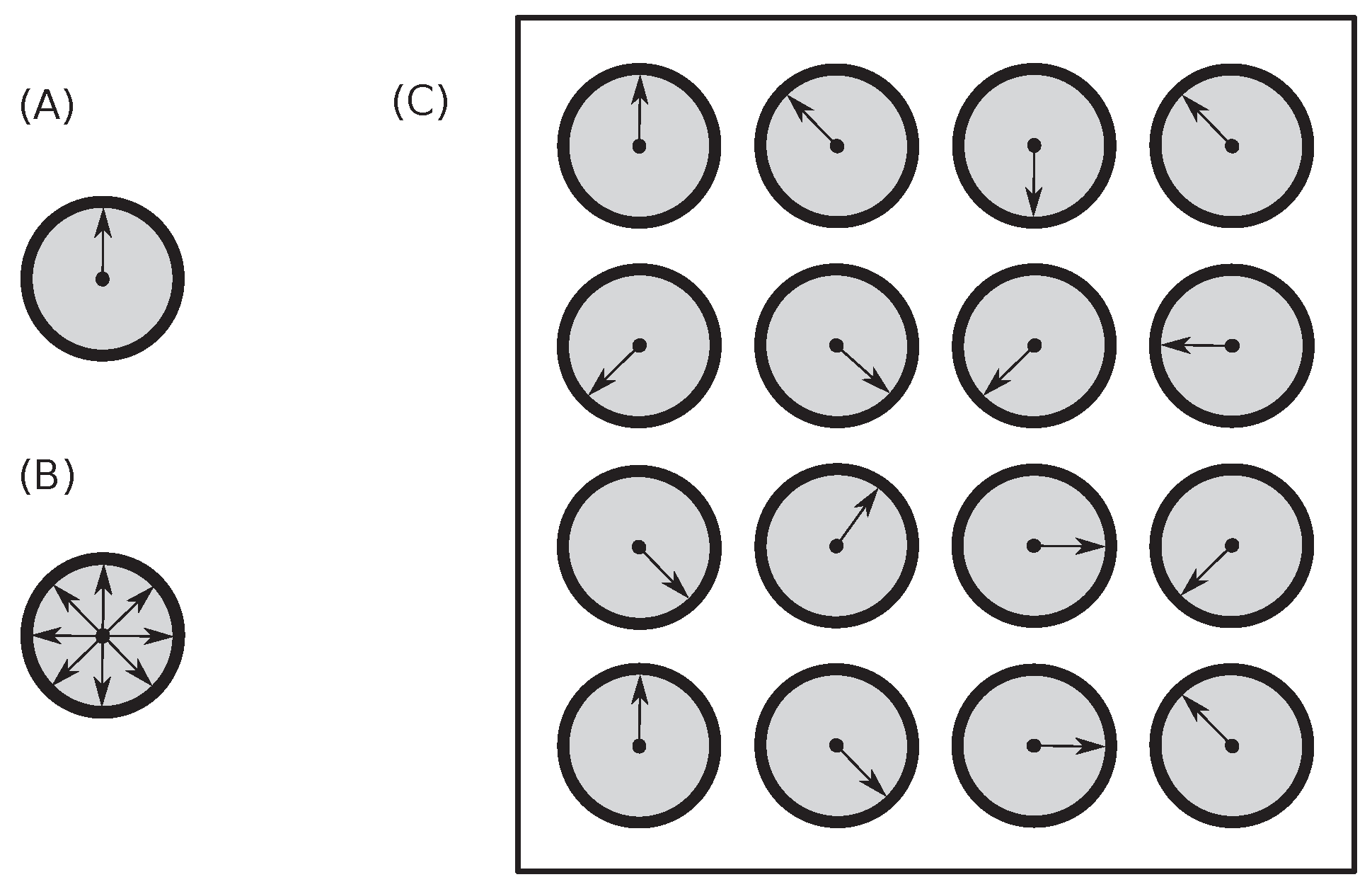
Figure 11.
An illustration of a single measurement as performed by the permutation entropy is shown. Three equidistant points, , with the spacing of the , intersect with the measured curve at three points (marked by circles) with values of . This particular measurement leads to the following ordering: . It is one from six possible.
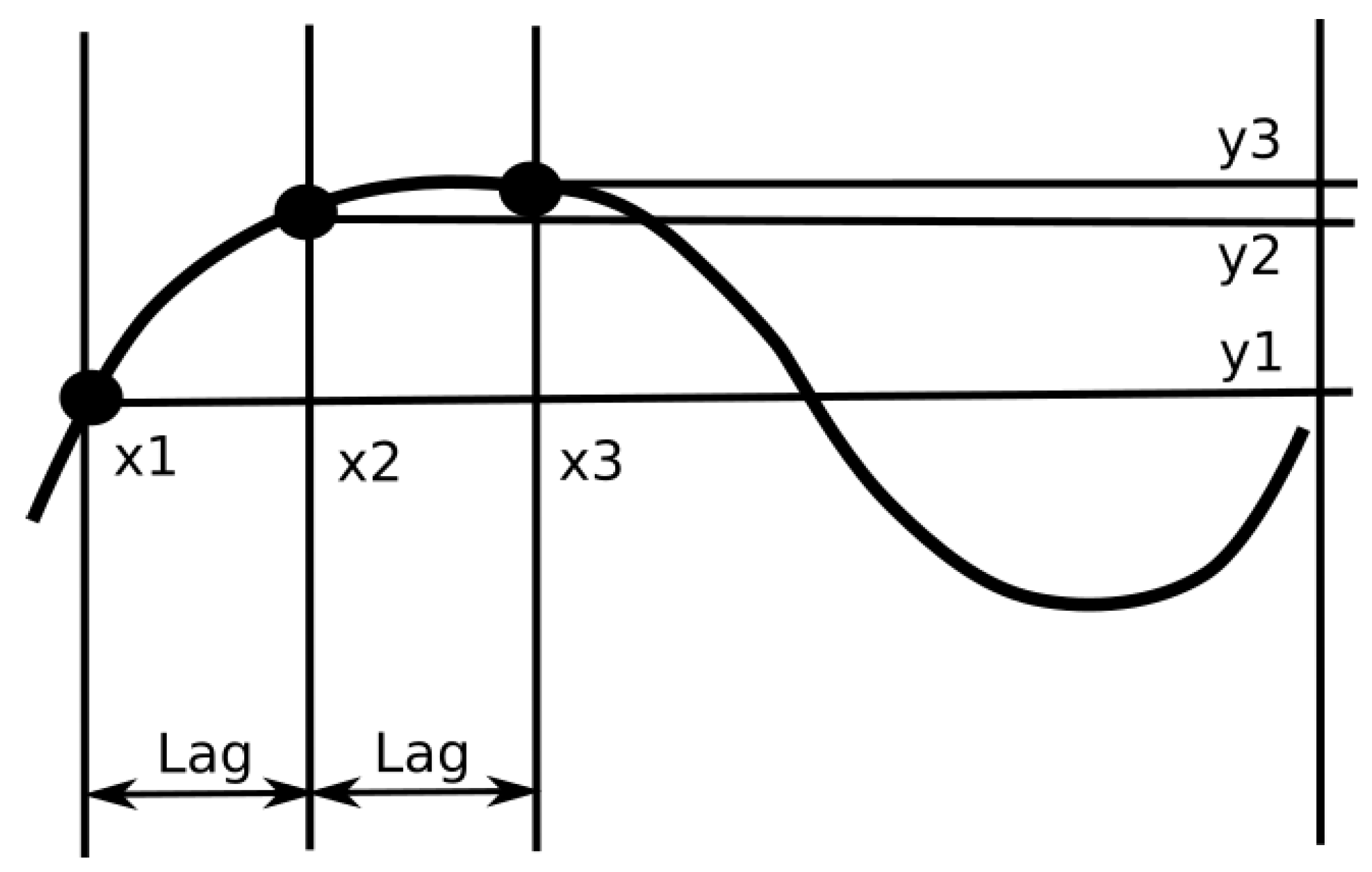
Figure 12.
A set of typical arrhythmogenic curves belonging to the ECG recording of the 1st rabbit (rabbit140731 in [52]) clearly demonstrates the presence of strong changes of entropy before and after the applications of methoxamine (; the first vertical line) and dofetilide ( and ) (compare to the typical non-arrhythmogenic behavior shown in Figure 13). Each parameter L of curves, which changes from 10 to 300, is displayed by a different color in the plot. The rabbit’s curves are displaying a strong reaction to drug interventions: the rabbit is incapable of coping with insults. Vertical lines mark the onset of the drug’s applications. Once drugs are applied, they are applied till the end of the measurement, or they get increased. Arrhythmia occur somewhere at times between 3500 and .
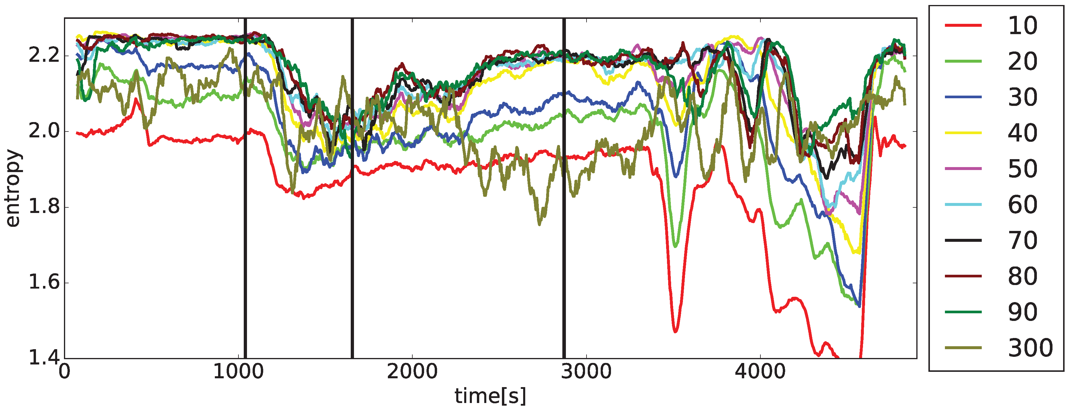
Figure 13.
A set of typical non-arrhythmogenic curves belonging to the ECG recording of the 2nd rabbit (rabbit130809 in [52]) clearly demonstrates the presence of mild changes of entropy after drug application times of methoxamine () and dofetilide (, , and ) (compare to the typical arrhythmogenic behavior shown in Figure 12). The rabbit’s curves are displaying a mild reaction to the drug interventions: the rabbit compensates for all insults. Vertical lines mark the onset of drug applications. Once drugs are applied, they are applied to the end of the measurement, or they get increased.
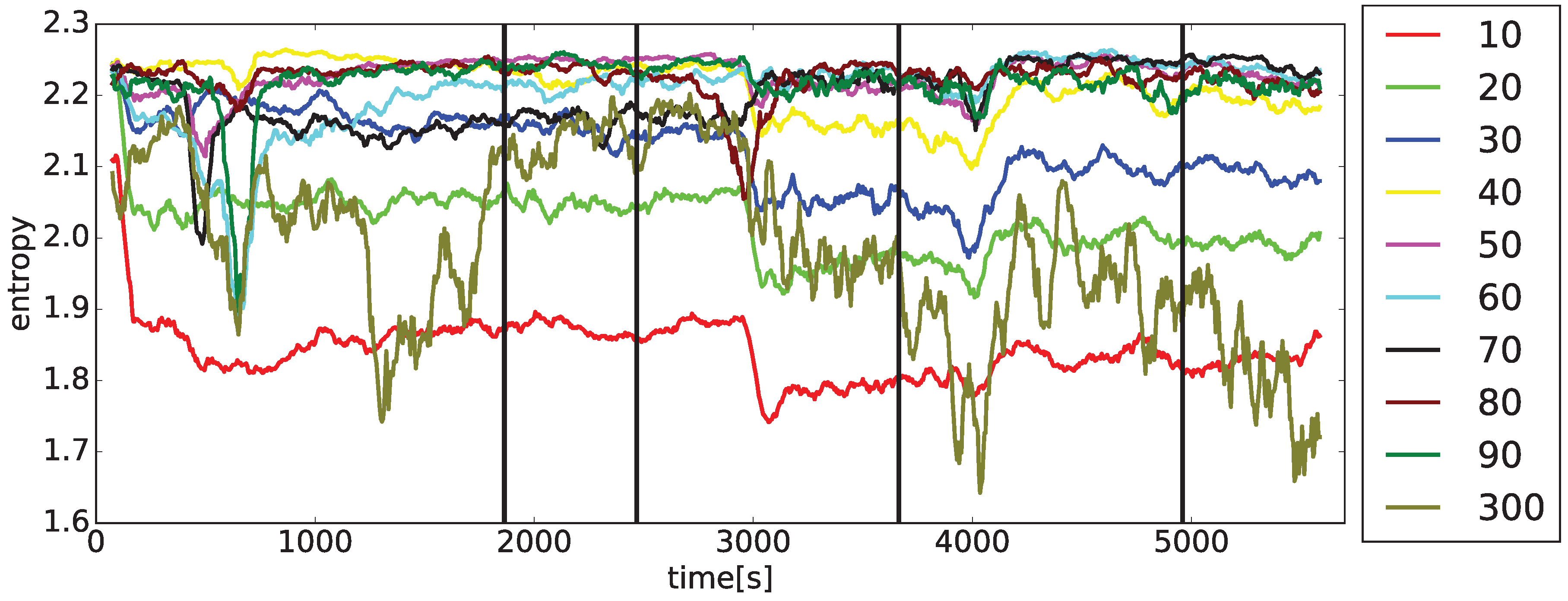
Figure 14.
curves for the 1st rabbit (same as in Figure 12) application times (black vertical lines) where two-second-long intervals of the ECG recordings (red vertical lines), which are taken at important times of evolution, are displayed in insets: (a) control interval at 700 sec (from the left-up corner in rows), (b) after the application of methoxamine at 1600 sec, (c) after the application of dofetilide at 2500 sec, (d) the onset of TdP at 3405 sec (the total length of 4 sec), (e) the onset of TdP at 3428 sec (the total length of 53 sec), (f) at the moment of a substantial decrease at 4300 sec. Black vertical lines mark the onset of drug applications. Once drugs are applied, they are applied till the end of the measurement or, they get increased. Red vertical lines define moments of five ECG insets displaying different stages of the heart physiology changes; ECG insets created by software [94].
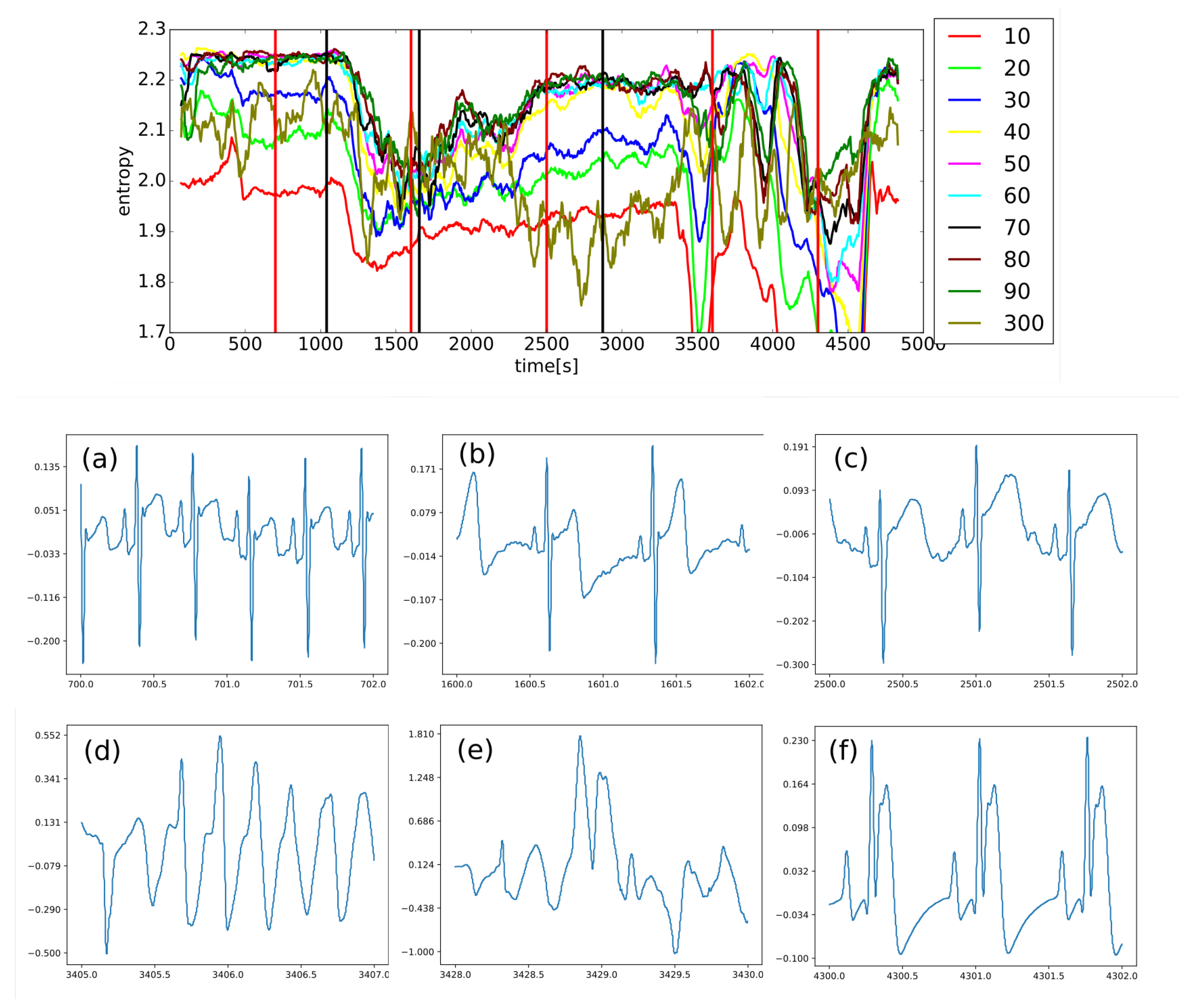
Figure 15.
The box plot displays important statistical features found in the control interval—before the application of any drug except anesthesia—for all 20 curves: rabbits not expressing arrhythmia (blue boxes) and those with arrhythmia (red boxes). Obviously, any discrimination between those two cases is impossible.
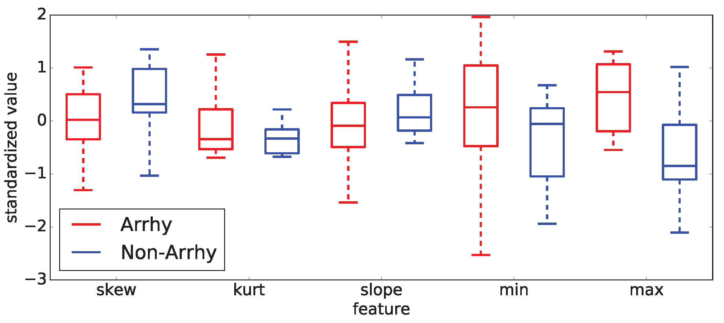
Figure 16.
The box plot displays important statistical features for all 20 curves found in the interval right after the application of methoxamine—the first given drug: rabbits not expressing arrhythmia (blue boxes) and those with arrhythmia (red boxes). Obviously, a discrimination between two cases—arrhythmogenic and non-arrhythmogenic rabbits—is impossible.
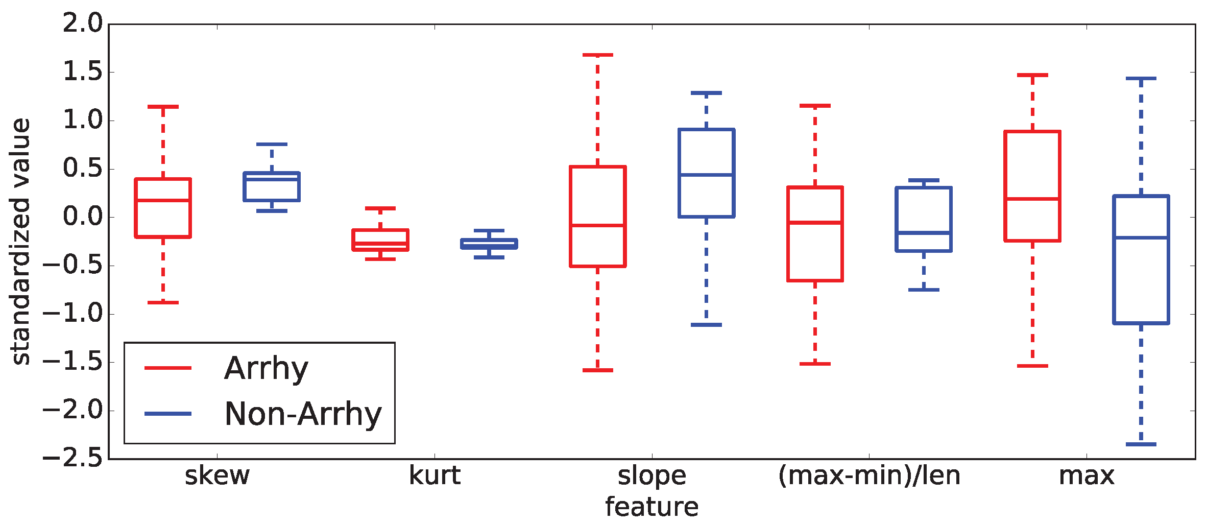
Figure 17.
(Left) An example of an important time moment indicated by a black line, which exists in the case of five sinus curves where all green curves are above zero and red ones are below zero. (Right) The previously identified important time moment do not exist in the case of 10 sinus curves. Here, green and red curves are mixed. Therefore, there is no way to distinguish two independent groups by the color, as in the previous case. This is why it is desirable to have as many evaluated curves as possible to rule out the result existing by pure chance.
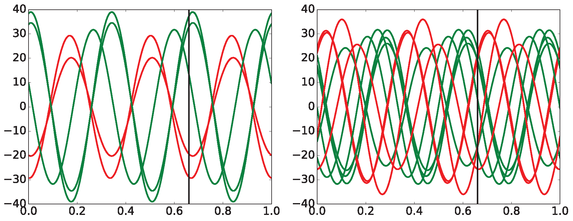
Figure 19.
All possible orderings of measuring points within permutation entropy —which is for simplicity referred to as within the whole paper—where the number of different measuring points is equal to are shown. In total, different combinations of vertical positions of those points exist in this type of . Hence, the number of bins collecting different events is equal to . With the increasing value of p, the number of all combinations grows very fast!

Figure 20.
The logistic regression takes N inputs that are arranged in the vector X and inserts them into a function containing an exponential function. This procedure gives a continuous output between 0 and 1, which might be considered as the probability of the classified event, i.e., how well it approximates 0 or 1.
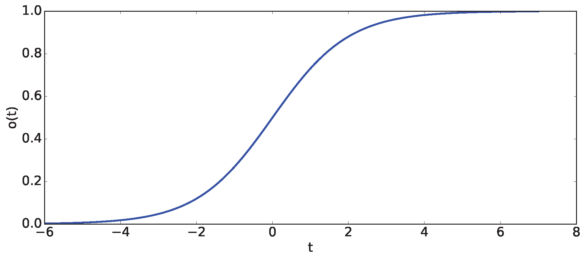
Figure 21.
A prototypical example of k-NN classification that is using only two features and and two classes A and B with just a few classified points. The currently classified point is depicted by the symbol ’X’ and is assigned to one of the classes according to the majority vote among its k-nearest neighbors: there are depicted two versions, either 3- or 5-NN in this example. Obviously, 3-NN and 5-NN cases give the opposite answers for the identical classified point ’X’.
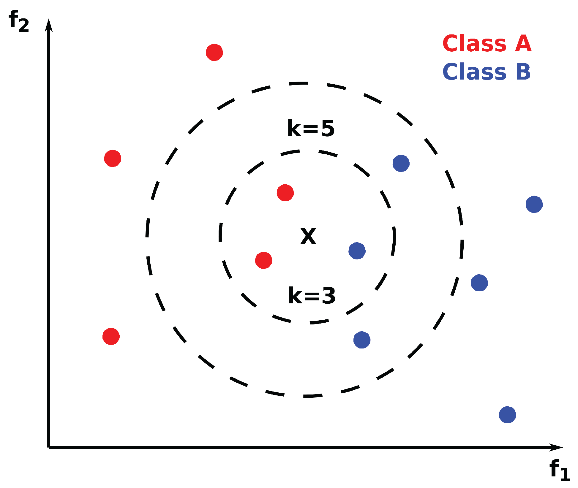
Figure 22.
A two-dimensional (2-D) example of an SVM machine is shown. The very principle of SVM is quite simple: (a) it takes data constituted by two features that are not separable by a single hyperplane (a line in 2-D), and (b) transforms it into another, usually higher-dimensional space—using a transformation function from the kernel—where data becomes separable. Here, just for clarity and simplicity, the transformed space has the same dimension as the original one. The hyperplane that is simultaneously the farthest away from both, separated groups is chosen; see arrows in the right panel.
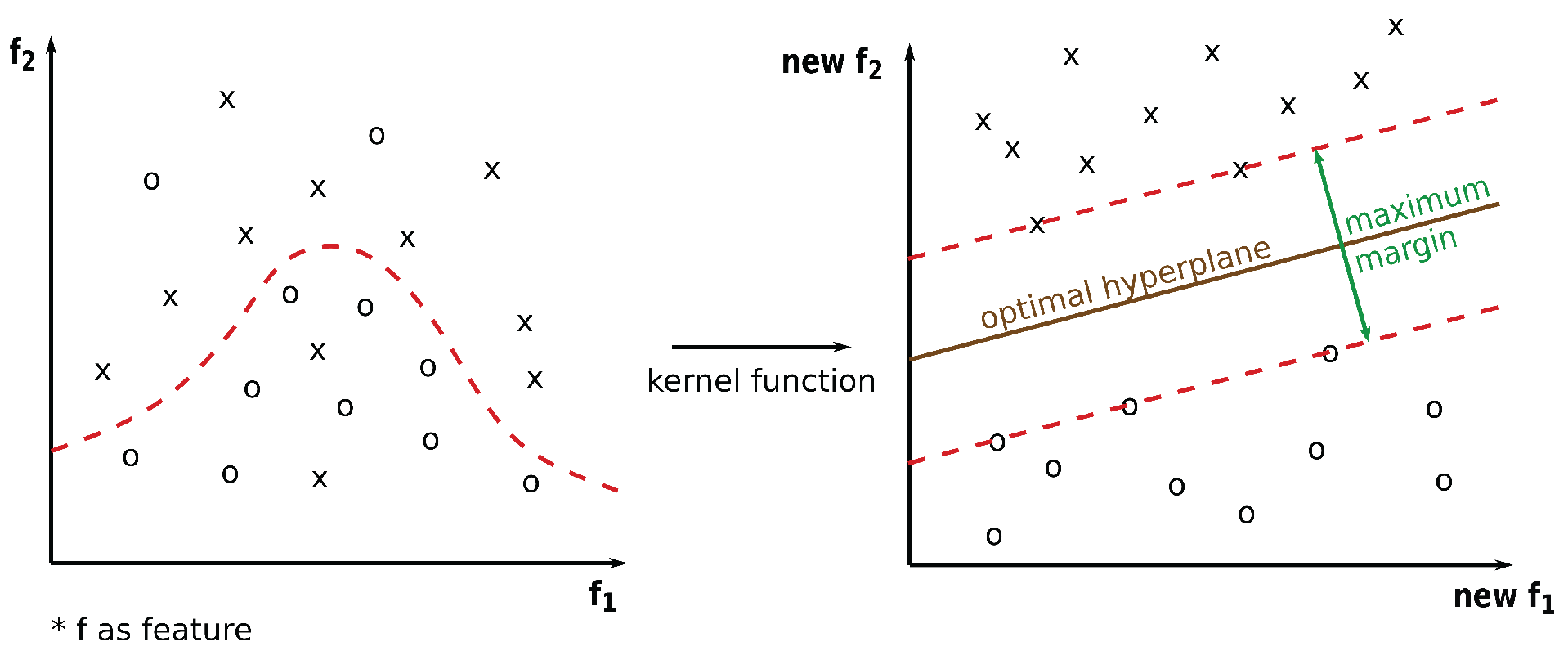
Figure 23.
An example of the recursive splitting of a decision tree: (Left panel) It depicts data partitioning in 2D space specified by features and with splitting points , , and . (Right panel) The standard description of the top-down recursive splitting of data using the decision tree—a simple, yet powerful way of data splitting.
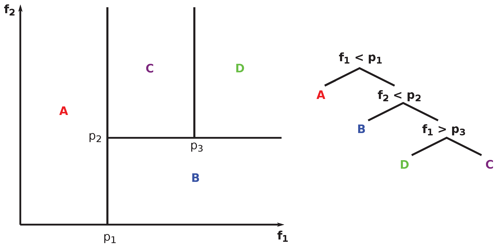
Figure 25.
All data that belongs to one rabbit stored at one table is providing simultaneous information about all features/time for all lags L at one place (two-dimensional case, 2-D). One of the feature sets (statistics, time, or something else) is used for one rabbit in one table. The fact that each rabbit has its own table(s) of values is very useful from the programming point of view because the horizontal and vertical viewpoints on data belonging to one rabbit can be easily retrieved from such tables.
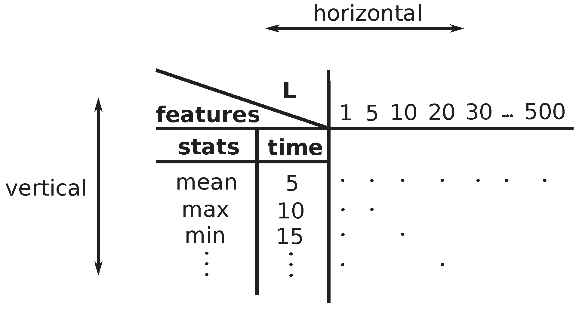
Figure 26.
(Left) The vertical viewpoint of one rabbit is an example of data and feature evaluation according to the table in Figure 25, where varying features are evaluated for fixed lag; as an example, the fixed shown. (Right) The same data is represented in the table for a given rabbit, where the line is displayed in the figure on the left in each horizontal plane. One column in the table represents one rabbit. The 3D plot on the left contains tables for all rabbits simultaneously—one table, one rabbit, one horizontal plane.
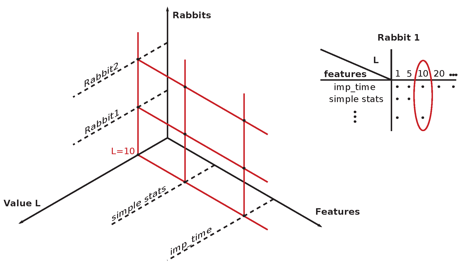
Figure 27.
(Left) The horizontal viewpoint on one rabbit is an example of data and features evaluation according to the table in Figure 25 where varying lags L are evaluated for the fixed feature, which is time t (fixed to the value ), in this specific example. (Right) The same data is shown in the 2D table for one rabbit, where the line is displayed in the 3D figure on the left within the horizontal plane belonging to the given rabbit. One horizontal line () in the 3D panel represents one rabbit. The 3D plot on the left contains tables for all rabbits simultaneously—one table, one rabbit, one horizontal plane.
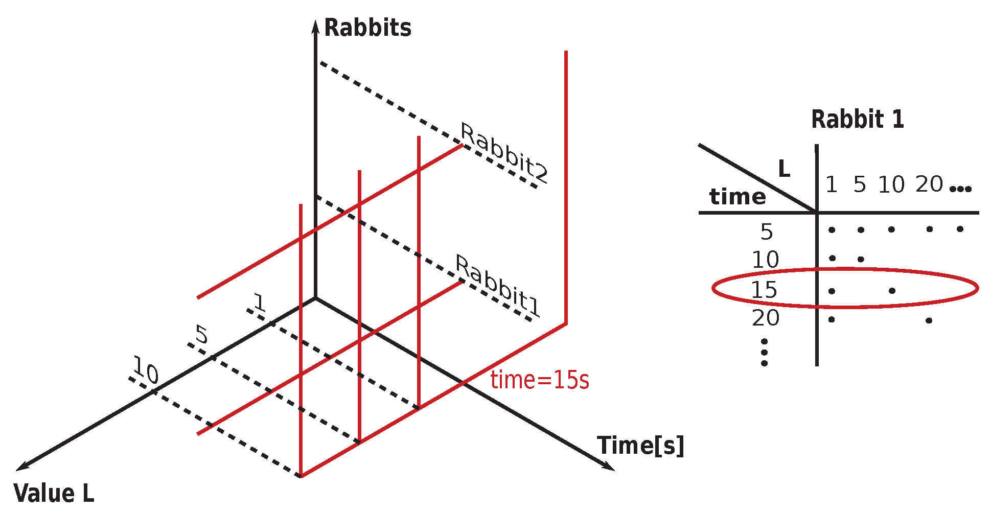
Figure 28.
time-slicing method where the features constituting a new point in 3D space are defined by the values of each curve (axis ) at the specified time-slice (t): (left) Three different curves of rabbits for the identical lag L (possibly more than three rabbits) displayed in a 2D plot, and (right) the same three lags from the left part displayed in 3D (possibly ND). This procedure of time-slicing steps is repeated several times (lying within a preselected range). As a result, there is created a set of multidimensional points (where time is the same for each time-slice, e.g., then ) that may or may not be successfully or not separated into two groups: arrhythmogenic and non-arrhythmogenic. It is possible to determine the most discriminating dimensions (i.e., values of L) using these multidimensional points.
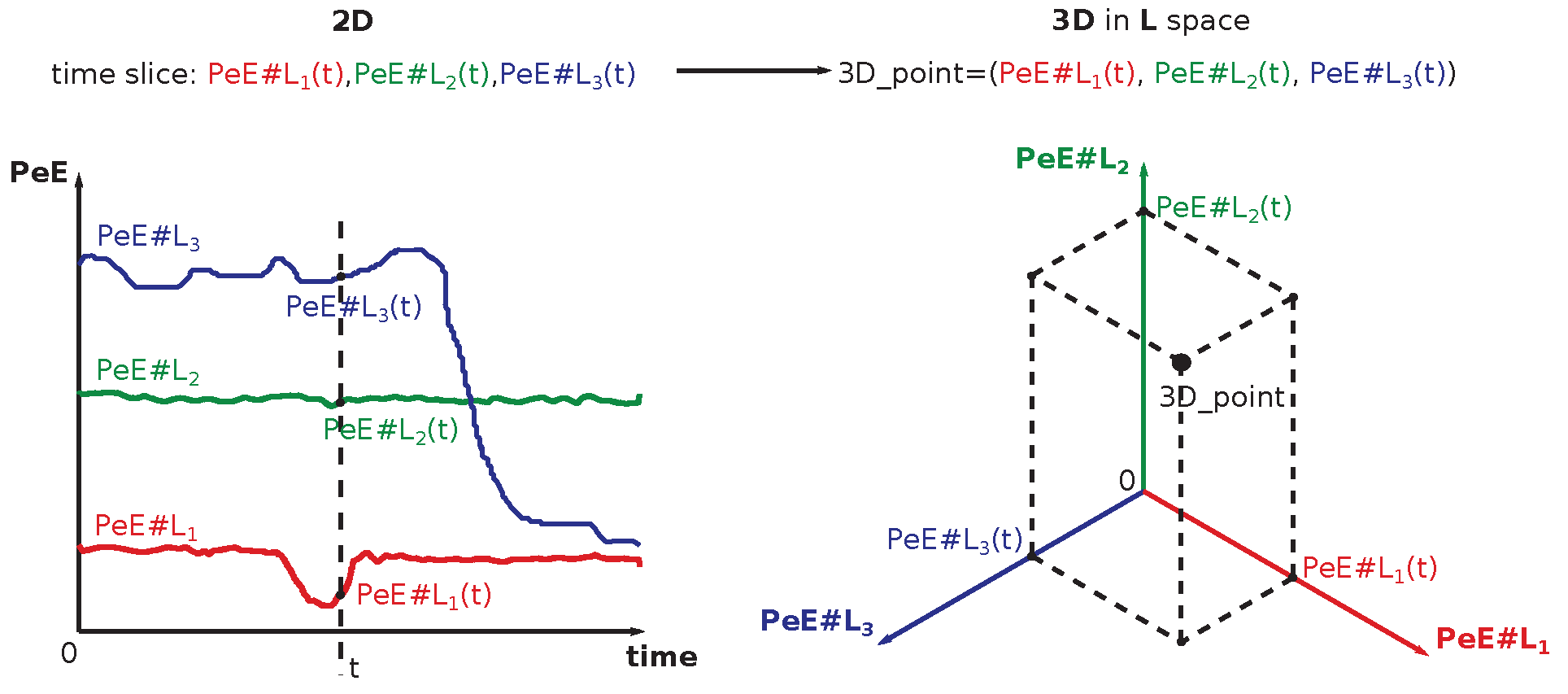
Table 1.
The terms macrostate and microstate are explained in an example of two dice throws: die A and die B. Each die can acquire one of the states independently—it gives in a total of possible combinations. A macrostate is given by the sum of values on both dice whereas microstates are all combinations of numbers on dice leading to this specific sum. The rhomboidal shape of the number of microstates represents the very principle of the second thermodynamic law (details in the text).
| Macrostates | Dice AB Configurations | #Microstates |
|---|---|---|
| (Sum) | ||
| 2 | 11 | 1 |
| 3 | 12, 21 | 2 |
| 4 | 13, 22, 31 | 3 |
| 5 | 14, 23, 32, 41 | 4 |
| 6 | 15, 24, 33, 42, 51 | 5 |
| 7 | 16, 25, 34, 43, 52, 61 | 6 |
| 8 | 26, 35, 44, 53, 62 | 5 |
| 9 | 36, 45, 54, 63 | 4 |
| 10 | 46, 55, 64 | 3 |
| 11 | 56, 65 | 2 |
| 12 | 66 | 1 |
Table 2.
The very existence of macrostates and microstates is explained on three dice throws: die A, die B, and die C. Each die can acquire one of the states independently—it gives in total possible combinations. A macrostate is the sum of states of all three dice, whereas microstates are all combinations of numbers on dice leading to this specific sum. The rhomboidal shape of the number of microstates is more pronounced within the central section.
| Dice Sum | Dice ABC Configurations | #States |
|---|---|---|
| 3 | 111 | 1 |
| 4 | 112, 121, 112 | 3 |
| 5 | 113, 131, 311, 122, 212, 221 | 6 |
| 6 | 114, 141, 411, 123, 132, 213, 231, 312, 321, 222 | 10 |
| 7 | 115, 151, 511, 124, 142, 214, 241, 412, 421, 133, 313, 331, 223, 232, 322 | 15 |
| 8 | 116, 161, 611, 125, 152, 215, 251, 512, 521, 134, 143, 314, 341, 413, 431, 224, 242, 422, 233, 323, 332 | 21 |
| 9 | 126, 162, 216, 261, 612, 621, 135, 153, 315, 351, 513, 531, 144, 414, 441, 225, 252, 522, 234, 243, 324, 342, 423, 432, 333 | 25 |
| 10 | 136, 163, 316, 361, 613, 631, 145, 154, 415, 451, 514, 541, 226, 262, 622, 235, 253, 325, 352, 523, 532, 244, 424, 442, 334, 343, 433 | 27 |
| 11 | 146, 164, 416, 461, 614, 641, 155, 515, 551, 236, 263, 326, 362, 623, 632, 245, 254, 425, 452, 524, 542, 335, 353, 533, 344, 434, 443 | 27 |
| 12 | 156, 165, 516, 561, 615, 651, 246, 264, 426, 462, 624, 642, 255, 525, 552, 336, 363, 633, 345, 354, 435, 453, 534, 543, 444 | 25 |
| 13 | 166, 616, 661, 256, 265, 526, 562, 625, 652, 346, 364, 436, 463, 634, 643, 355, 535, 553, 445, 454, 544 | 21 |
| 14 | 266, 626, 662, 356, 365, 536, 563, 635, 653, 446, 464, 644, 455, 545, 554 | 15 |
| 15 | 366, 636, 663, 456, 465, 546, 564, 645, 654, 555 | 10 |
| 16 | 466, 646, 664, 556, 565, 655 | 6 |
| 17 | 566, 656, 665 | 3 |
| 18 | 666 | 1 |
Table 3.
The procedure used to find the most suitable methodology that would eventually enable prediction of incoming heart arrhythmias using one-lead ECG recordings on a rabbit model .
Table 3.
The procedure used to find the most suitable methodology that would eventually enable prediction of incoming heart arrhythmias using one-lead ECG recordings on a rabbit model .
| Used method | Reasons and Achieved Results (Done by) | Success |
|---|---|---|
| Study of complex systems apps in medicine | This phase was quite intensive and extensive [63] (not reported). (J.K.) | . |
| Analysis of usefulness of various entropies | Extensive study of all existing entropy measures and their applications. Foundations of this research rely on deep understanding of entropy measures [63] & Section 1. (J.K.) | . |
| Permutation entropy | This measure was detected as the most suitable for measuring short runs of ECG recordings; see Section 6.2. It serves as the input into classification. (J.K.) | Yes |
| Heart rate variability | Had been studied in depth and found useless in prediction of arrhythmias (not reported). (J.K.) | No |
| Simple Statistics | Found insufficient in the prediction of arrhythmias; see Section 4. (J.K.) & (D.B.) | No |
| Advanced Statistics | Found insufficient in prediction of arrhythmias; see Section 4. (D.B.) | No |
| Machine Learning Methods | Selected methods displayed relatively high sensitivity in the prediction of arrhythmias; see Section 4 and Appendix C. (D.B.) | Yes |
Table 4.
A concise list of typical arrhythmia types observed on ECG recordings of humans; compare to the schematic depiction of a single beat on an ECG curve, Figure 5, and a normal ECG curve, Figure 6.
| Type of Arrhythmia | Description |
|---|---|
| Torsades de Pointes (TdP) | A TdP arrhythmia is typically induced by the application of drugs both medical and recreational. Both types affect the functioning of ion channels that are utilized by cardiomyocytes to propagate action potential through them. Distribution of velocities of propagation of action potential is varying across the thickness of the heart walls. This triggers arrhythmia with a meandering focal point; see Figure 7. |
| Ventricular Tachycardia (VT) | A VT typically occurs in structurally damaged hearts after cardiomyopathy, heart infarction, heart inflammation with re-modulation of cardiomyocytes, or due to a genetic disease. All of those causes are leading to permanent structural changes of cardiomyocytes and/or the conductive system that triggers arrhythmia events with a fixed focal point. Structural changes lead to dispersion of action potential propagation speeds; see Figure 8. |
| Ventricular Fibrillation (VF) | VFs are similar to VTs, with the difference that there are simultaneously operating several focal points, which act as surrogate pacemakers; see Figure 9. |
| Premature Ventricular Contraction (PVC) | PVCs are heart contractions randomly initiated in ventricles of hearts. They, when doubled, and even more when tripled, can trigger a run of TdP, VT, or VF event; see Figure 10. |
Table 5.
A comprehensive list of abbreviated names of all features and their respective descriptions used throughout the paper is given—it provides navigation within all hypothesis tests. The full set of data is huge. Therefore, selected intervals, which are narrowing the full set of data, are used instead. The importance of each set of features (which are acquired during subsequent evaluation) is reflected by the number of stars (more stars mark more important results). Results are grouped into the following groups: ’***’ as the best (ARARS ≥ 90%), ’**’ as sufficient (80% ≤ ARARS < 90%), ’*’ as average (75% ≤ ARARS < 80%), ’ ’ not useful (no star) (ARARS < 75%).
| Features | Description |
|---|---|
| ISI_Top5-TM*** | top five important time moments discovered by Random Forest for each sub-interval |
| ISI-RM_Top5-TM** | top five important time moments discovered by Random Forest for each sub-interval with rolling mean |
| ISI | all values of each sub-interval |
| ISI-RM* | all values of each sub-interval with rolling mean |
| OC_SSF* | simple statistical features of each original |
| OC_ASF** | simple + advanced statistical features of each original |
| ISI_SSF* | simple statistical features of each sub-interval |
| ISI_ASF* | simple + advanced statistical features of each sub-interval |
| OC_Top5-ASF** | top five important statistical features (simple + advanced) discovered by Random Forest for the original s |
| ISI_Top5-ASF*** | top five important statistical features (simple + advanced) discovered by Random Forest for each sub-interval |
| Top5-L-ISI | all values of each sub-interval of top five important values of L parameter discovered by Random Forest for the appropriate sub-interval |
| Top5-L-ISI_Top5-TM** | top five important time moments of top five important values of L parameter discovered by Random Forest for each sub-interval |
| Top5-L-OC_Top5-ASF** | top five important statistical features (simple + advanced) of the original s for the selected values of the L parameter. These values are selected as the union of the top five important values of the L parameter discovered by Random Forest for each sub-interval. |
| MSI | merge of all values of control and methoxamine intervals together for each |
| MSI_Top5-TM*** | merge of the top five important time moments of control and methoxamine intervals together for each |
| MSI_Top5-TM & OC_ASF*** |
top five important time moments of control and methoxamine intervals merged together for each with subsequent merging with all statistical features (simple + advanced) computed for the appropriate original (not dissected) (i.e., control_imp_time + methoxamine_imp_time + ostats) |
| ISI_Top5-TM & OC_ASF*** |
merging the top five important time moments of each sub-interval with all statistical features (simple + advanced) computed for the appropriate original (i.e., control_imp_time + ostats, methoxamine_imp_time + ostats) |
| MSI_Top5-TM & MSI_Top5-TM-ASF*** |
top five important time moments of control and methoxamine intervals merged together for each with subsequent merging with all statistical features (simple + advanced) computed for this merged important time moments (i.e., control_imp_time + methoxamine_imp_time + cstats) |
| ISI_Top5-TM & ISI_ASF*** |
merging the top five important time moments of each sub-interval (control or methoxamine) with all statistical features computed for the appropriate sub-interval (i.e., control_imp_time + control_stats, methoxamine_imp_time + methoxamine_stats) |
| ISI_Top5-TM & ISI_Top5-ASF*** |
merging the top five important time moments of each sub-interval (control or methoxamine) with important statistical features computed for the appropriate sub-interval (i.e., control_imp_time + control_imp_stats, methoxamine_imp_time + methoxamine_imp_stats) |
| ISI-DFT_Top5-C*** | The top five important DFT coefficients (15 real values and 15 imaginary are merged together and the top five from them are selected) were evaluated for each sub-interval. Important time moments were identified by Random Forest. |
| ISI-DFT_Top5-TM** | Top five important time moments (identified by Random Forest) of each sub-interval, whereas curve, specified by values in the appropriate sub-interval, was reconstructed by the first ten DFT coefficients. |
| ISI-DWT_Top10-C*** | Ten most significant DWT coefficients of each taken in absolute value sub-interval. The coefficients were sorted in descending order. |
| ISI-DWT_Top5-TM*** | Top five important time moments (identified by Random Forest) of each sub-interval, whereas curve, specified by values in the appropriate sub-interval, was reconstructed by ten most significant in absolute value DWT coefficients. |
| MSI_Top5-TM-ASF | All statistical features (simple + advanced) computed for the merged top five important time moments of sub-intervals (tested only with MLP). |
Table 6.
An overview of the best results (ARARS score > 75%), which are achieved for combinations of features and ML algorithms is provided for easier orientation. Results are sorted for both control and methoxamine groups; it is done according to used features, methods, and lags L. Values of lag L, which are in bold within the table, are observed more frequently among all lags L—that is, all for the specified ML methods and the combination of features.
| Features | Used algorithms | Used L | |
|---|---|---|---|
| Control | methoxamine | ||
| ISI_Top5-TM | SVM | 1, 100, 30, 300, 40, 500, 60 |
10, 100, 20, 200, 30, 300, 40, 5, 50, 500, 60, 70, 90 |
| RF | 300, 400, 500, 90 | 100, 5, 500 | |
| k-NN | 100, 30, 500, 60 |
10, 100, 20, 300, 40, 400, 5, 50, 500, 90 |
|
| LR | 100 | 10, 200, 300, 5, 500, 90 | |
|
OC_Top5-ASF |
SVM | 10, 20, 300, 40, 5, 50, 500, 90 | |
| SVM, RF, k-NN, LR | RF: 40 LR: 10, 40 k-NN: 10, 300, 5, 50, 90 SVM: 10, 20, 300, 40, 5, 50, 500, 90 |
||
| OC_ASF | SVM | 10, 40, 50 | |
| ISI_Top5-ASF | SVM | 20, 300 | 40, 60 |
| ISI_Top5-TM & ISI_Top5-ASF | SVM, RF, k-NN, LR | RF: 300 LR: 300, 60, 80 k-NN: 1, 300 SVM: 20, 30, 300, 500, 60, 80 |
RF: 100 LR: 200, 300, 400, 500 k-NN: 10, 20, 500, 60, 80 SVM: 10, 200, 30, 300, 400, 500, 60, 70, 80, 90 |
| ISI-DFT_Top5-C | SVM | 40, 400, 5, 90 | 1, 20, 200, 30, 80 |
| ISI-DWT_Top10-C | SVM | - | 10, 40, 60 |
Disclaimer/Publisher’s Note: The statements, opinions and data contained in all publications are solely those of the individual author(s) and contributor(s) and not of MDPI and/or the editor(s). MDPI and/or the editor(s) disclaim responsibility for any injury to people or property resulting from any ideas, methods, instructions or products referred to in the content. |
© 2025 by the authors. Licensee MDPI, Basel, Switzerland. This article is an open access article distributed under the terms and conditions of the Creative Commons Attribution (CC BY) license (http://creativecommons.org/licenses/by/4.0/).
Copyright: This open access article is published under a Creative Commons CC BY 4.0 license, which permit the free download, distribution, and reuse, provided that the author and preprint are cited in any reuse.


