Submitted:
18 August 2025
Posted:
19 August 2025
You are already at the latest version
Abstract
The paper describes an enhanced version of a scheme originally designed by the current author to enable one to improve the quality of one’s own wireless communications, over a given frequency (or frequencies), when in the presence of inter‑modulation distortion (IMD). The IMD is that generated by one’s own power amplifier (PA), when operating over an adjacent band of frequencies, and arises as a result of the non‑linear nature of the PA when engaged in the transmission of modulated multi‑carrier (MMC) signals. The IMD appears in the form of inter‑modulation products (IMPs), these occurring at multiple frequencies which may potentially coincide with that of one’s own communication. The new version – which, like the original scheme, efficiently predicts the locations and strengths of the IMPs and, when coincident with the communication frequency, clears the IMPs from that frequency – overcomes the limitations of the original scheme. That is, it enables one to handle more sophisticated signal types whereby both bandwidths and powers of the signal components may now be arbitrarily defined. Also, it extends the scheme’s applicability to multiple zones of distortion, this resulting in the need to handle 2nd‑order and 4th‑order IMD terms as well as the 3rd‑order and 5th-order terms originally addressed.
Keywords:
FFT
; IMD
; IMP
; MMC
; PA
; SWAP
1. Introduction
A problem exists with the use of power amplifiers (PAs) for modern wireless communications due to the non-linear nature of their transfer characteristic. More specifically, when a single PA is used for the transmission of modulated multi-carrier (MMC) signals – as encountered with orthogonal frequency division multiplexing (OFDM) or multi-carrier spread spectrum (MC-SS) systems [1] – the PA non-linearity may result in the generation of undesirable inter-modulation distortion (IMD). This is expressed in the form of inter-modulation products (IMPs) which may occur at various frequencies distributed across the spectrum. This can be serious when strong IMPs [2] occur at that frequency (or frequencies) over which one wishes to communicate.
To address this problem, an IMD prediction and channel clearance scheme [3] was devised (based upon the paper by Baruffa and Reali [4]) by the current author which enabled one, given the known carrier locations, to first predict the locations/strengths of the dominant IMPs arising from the use of the PA and, subsequently, to be able to adjust the locations of one or more of those carriers causing the IMD. The scheme made efficient use of polynomial arithmetic/algebraic techniques and a fast Fourier transform (FFT) routine [5,6] in order to address the prediction problem – see Figure 1. This enabled the arithmetic-complexity of the original combinatorial problem, for simple combinations of IMD, to be approximated by O(M×logM), where ‘M’ is the number of channels that encompass the IMD region of interest. The computational efficiency of the solution to the prediction problem was subsequently exploited to enable the channel clearance algorithm – see Figure 2 – to be designed with an arithmetic-complexity of just O(M×log2M). The scheme has successfully enabled those IMPs preventing or degrading communications to be sufficiently reduced in strength – where strength, for a given frequency channel, simply refers to the number of IMPs occurring within that channel – as to enable reliable communications to take place.
The scheme currently suffers from three serious limitations, however, in that three key assumptions need first to be made, namely that for the MMC signal all signal components: a) possess the same bandwidth – this being equal to the channel bandwidth; b) possess the same amplitude and modulation type so that each IMP, as a consequence, possesses the same power; and finally that: c) only the first zone of the pass-band non-linearity (i.e., that region containing the first harmonics of the non-linear PA outputs and referred to hereafter as just the ‘first zone of distortion’) of the PA [7] is of relevance, so that the potentially significant zero’th and higher order zones of distortion are not catered for by the scheme.
To address these problems, therefore, an enhanced version of the IMD prediction and channel clearance scheme has been devised which, in order to avoid having to replicate material, should be studied in conjunction with the original IET paper [3]. A simple polynomial model of the PA is first described in Section 2, as this will prove essential in enabling the original scheme to be extended to cater for more sophisticated signal types, as discussed in Section 3, which may now possess both arbitrary signal bandwidths and powers. This is followed in Section 4 by a discussion of its applicability to multiple zones of distortion which may well overlap or even coincide. This necessitates being able to deal with 2nd-order and 4th-order IMD terms as well as the 3rd-order and 5th-order terms catered for by the original scheme. Complexity issues and simulation results are then discussed in Section 5 and Section 6, respectively, followed by a summary and conclusions in Section 7. Finally, a description of parameters derived from the application of the PA model is given in the Appendix.
2. Polynomial Modelling of Non-Linear PA Behaviour
Before discussing how the applicability of the IMD predictor might be extended to cater for signal types that are more sophisticated than those originally addressed, it is necessary that a brief account be given as to how the transfer characteristic of the proposed PA might be modelled. The transfer characteristic is dependent upon a number of parameters, including the input signal bandwidth and power level and the operating temperature. When amplifying the signal to be transmitted, the PA acts in a non-linear fashion with the level of non-linearity increasing with the values of the driving parameters.
Memory effects associated with the PA performance are attributed to a number of factors, including filter group delays, the frequency response of matching networks, non-linear capacitances of the transistors and the response of the bias networks. Any operational PA will have memory, meaning that its output will be a function not only of the current input, but also of the past inputs and outputs. With the case of a MMC signal – as is of interest here – the wider the separation in frequency between the components, the wider the bandwidth of the signal and the greater the effect of such memory on PA performance is likely to be.
A number of polynomial-based representations are possible for dealing with the frequency-dependent modelling of the PA behaviour, as required for dealing with memory effects, such as that of the memory polynomial [8]. For the purposes of this research, however, a much simpler frequency-independent approach is taken which is both conceptually and computationally simple, whereby the PA output, y(t), is written in terms of the PA input, x(t), via the polynomial expression
where {ck}, for ‘k’ ranging from 0 up to K, is the set of polynomial coefficients and ‘K’ corresponds to the maximum IMD order of interest. The evaluation of the polynomial coefficients is itself a potentially complex task, however, relying upon the availability of accurate knowledge of the PA’s transfer characteristic (in terms of both amplitude and phase). An attractive approach to the derivation of the modelling coefficients, particularly for more complex formulations as typified by the memory polynomial, is via the use of a genetic algorithm (GA) [9] whereby measured PA data sets, in the form of input data segments and their corresponding output spectra, are used as truth data in the GA’s cost or objective function.
y(t) = c0 + c1.x(t) + c2.x2(t) + … + cK.xK(t) (1)
3. Catering for More Sophisticated Signal Types
With the original IMD prediction and channel clearance scheme it was necessary to make three simplifying assumptions, the first two of which were that the carriers for all components of the MMC signal: 1) were centred on multiples of some pre-defined channel bandwidth; and 2) possessed the same amplitude and modulation type so that the IMPs possessed the same power. This section, which forms the heart of the paper, looks into how these first two restrictions might be effectively overcome without incurring too great a computational cost. The question of how to handle arbitrary signal bandwidths is discussed first, as this leads on naturally to the question of arbitrary signal powers. The third restriction, namely: 3) that relating to the PA’s zones of distortion, is to be discussed in Section 4.
3.1. Arbitrary Signal Bandwidths
Suppose, for ease of illustration, that a signal comprises just two tonal components with each centred on some multiple of the channel bandwidth. Then each signal component (which possesses an effectively zero bandwidth) will reside within a single channel and when passed through a non-linear PA the two will combine to produce, on output, an IMP that will in turn be centred on some multiple of the channel bandwidth and reside within a single channel. When one or both of the signal components possesses modulation, however, each such component will possess a finite non-zero bandwidth which may be approximated by some integer multiple of the channel bandwidth – note that the channel bandwidth must be consistent with the narrowest signal bandwidth of interest. As a result, for a particular order of IMD, the resulting distortion will spread over a number of consecutive channels, with the number of such channels being determined by the bandwidths of the signal components involved and the order of the IMD – the higher the order the greater the number of excited channels. This is due to the fact that the PA non-linearity will result in the multiplying together of signals in the time domain which is equivalent, via the Circular Convolution Theorem, to the convolving of their spectra in the frequency domain. The centre frequency of the resulting IMD will be an integer function – according to the order of the IMD involved – of the centre frequencies of the signal components being combined.
The above idea generalises in a straightforward fashion to cater for the case where multiple signal components are combined via the non-linearity of the PA to produce the unwanted distortion. Thus, when the IMD is of arbitrary order, ‘k’, the number of signal components that may combine in this way to produce the distortion will range from just ‘2’ up to a maximum of ‘k’ [3].
To illustrate the idea with an example, let us consider the case of 3rd-order IMD for the first zone of distortion with the carrier signal combination as represented by the channel weights {+2,-1} [3]. Suppose that the first signal component possesses a centre frequency of f1 and a bandwidth covering approximately W1 channels, whilst the second possesses a centre frequency of f2 and a bandwidth covering approximately W2 channels. Then the resulting IMD will be centred on the frequency
and will spread across a frequency band of maximum width
fIMD = 2×f1 - f2 (2)
WIMD 2×W1 + W2, (3)
with the strength of the individual IMPs within the region of distortion varying according to how the different modulations interact with one another.
For the proposed scheme to be able to cater for such arbitrary signal bandwidths – that is, for arbitrary integer multiples of the channel bandwidth – it is necessary that each signal component be treated as comprising a number of consecutive single-channel sections where the power content of all the sections sum to that of the corresponding signal component. To cater for this, the signal component frequencies, as defined by the binary-valued coefficients of the indicator polynomial [3], need to be modified to reflect the presence of all sections of each signal component, whilst the tabulated signal component amplitudes need to reflect both the power and spectral shape of each signal component with entries being provided for each single-channel section of each signal component.
Thus, it is evident that in being able to handle arbitrary signal bandwidths it is also necessary that the proposed scheme should be able to handle arbitrary signal powers, since certain IMD regions of interest may now be spread over multiple channels, as a result of the modulation present on certain of the signal components, rather than over a single channel.
3.2. Arbitrary Signal Powers – Two Amplitude Levels
The standard approach to dealing with the question of arbitrary signal powers is as outlined in [4]. This involves, for a given set of channel weights, fitting a sum of products of Bessel functions to an accurately measured PA transfer function. However, the approach is complex, computationally intensive and only applicable to the case of a memoryless PA. An empirical approach is therefore adopted whereby parameters derived from the signal information – that is, from the component frequencies and amplitudes – may be dynamically and efficiently updated, on the fly, for subsequent processing by the IMD prediction and channel clearance scheme.
Suppose that a representative set of polynomial coefficients is defined that enables the PA to generate ‘realistic’ levels of distortion for each IMD order – see Appendix. Suppose also that the signal components partition into just two distinct sets: a set S1 containing all those components possessing an amplitude of approximately ‘m1’ and a set S2 containing all those components possessing an amplitude of approximately ‘m2’, where
m2 < m1, (4)
so that all the signal components may be said to belong to a set S12 where
S12 = S1 S2. (5)
The first task to be addressed is how to exploit the combined use of both the PA model and the IMD predictor so as to obtain an expression for the IMD distribution due to the contents of the set S12, given that the IMD predictor, on its own, is only able to operate with the contents of set S1 or set S2 and with the fixed amplitude set equal to one. For a fixed order of IMD, ‘k’, let us denote the partial distributions associated with the sets S1 and S2 by and , respectively, with the estimated partial distribution for S12 given by . The required composite IMD distribution derived from all those orders of interest will be straightforwardly obtained through summation of the appropriate fixed-order distributions, e.g., by adding the fixed-order distributions for ‘k’ varying from 2 to 5, where each such distribution is in turn obtained from the summation of its own partial distributions. The strength of the distribution, for a given channel, may now be regarded as an approximation to the IMD power content of the channel, rather than the simplistic IMP count of the original scheme.
When using the PA model for a fixed order of IMD, the energy obtained from the summing of the squared amplitudes of a set of consecutive time-domain output samples will be considered to be equivalent (up to a scaling factor) – via Parseval’s Theorem [10] – to that obtained in the frequency domain, via the IMD prediction algorithm, from the summing of the squared amplitudes of the resulting IMPs. The PA model may therefore be used to obtain scaling factors for determining the relative level of the partial distributions, and , as the IMD predictor alone is clearly not able to do so. This is unlike the situation with the PA model which is able to deal simultaneously with multiple signal components possessing different amplitudes, thereby justifying it’s use as ‘truth’ data in facilitating adjustment of the partial distribution levels.
Note that different scaling factors will need to be computed for each fixed order of IMD to be catered for by the PA model, with the scaling factors ensuring that the energy present in each fixed-order distribution produced by the IMD predictor is consistent with that present in the corresponding PA model output. All the partial distributions of each fixed-order distribution are assumed, hereafter, to have been suitably normalised to account for the energy levels of the corresponding PA model outputs – see Appendix.
Before proceeding, it should also be noted – from the definitions given in Appendix – that for any pair of arguments, ‘mx’ and ‘my’, and order of IMD, ‘k’, the associated partial distributions may be connected via the ‘power-based’ equivalence relationship
, (6)
for an arbitrary set, Sn, so that two partial distributions defined over the same set of signal components but with different amplitudes are obtainable, one from the other, via a simple scaling factor provided by the PA model. Alternatively, when one of the two partial distributions possesses an argument of one, as with the original scheme, the distributions may be connected via the energy equivalence described by Parseval’s Theorem so that . (7)
These properties are now exploited so that an approximation to the term may be obtained. Let this term be first expressed as
, (8)
where represents the partial distribution comprising all those IMPs that are derived from the combining of signal components from both S1 and S2 – that is, there must be at least one signal component from each set. Let the last term in the above expression be written as
, (9)
for some argument – this representation is possible from Eqtn. 6. Then the requirement is to select a value for that results in an energy level for that is consistent with that derived from the corresponding PA model outputs. However, it should be noted that although and will possess the correct spectral shapes, the adjustable component, , will not necessarily do so as individual IMPs may be either smaller or larger than they should actually be. The aim here is simply to achieve a more accurate estimate than that originally obtained via the fixed-amplitude approximation.
To derive the value of the parameter needed for this approximation one may use the PA model – with the energy present in the model output for order ‘k’ distortion being denoted by – whereby (10)
with
(11)
and the parameter ‘’ being thus expressed as
(12)
for each fixed value of ‘k’.
3.3. Arbitrary Signal Powers – Three Amplitude Levels
To generalise the above results from the use of two amplitude levels to three amplitude levels, suppose that sets S3 and S123 are introduced, where set S3 contains all those signal components possessing an amplitude of approximately m3, whereby
m3 < m2 < m1, (13)
and set S123 contains all those signal components belonging to sets S1 or S2 or S3, so that
S123 = S12 S3 = S1 S2 S3. (14)
Then, adopting the same approach as before, the partial distribution for the set S123 may be written as
(15)
where
, (16)
for some argument – this representation, as with that for Eqtn. 9, is possible from Eqtn. 6. Then the requirement is to select a value for that results in an energy level for that is consistent with that derived from the corresponding PA model outputs. However, it should be noted that although , and will possess the correct spectral shapes, the adjustable components, and , will not necessarily do so since individual IMPs, as with the case of two amplitude levels, may be either smaller or larger than they should actually be.
The value of the parameter , like that of , may be expressed in terms of the PA model outputs, with
(17)
for each fixed value of ‘k’.
3.4. Discussion
The results derived in the previous two sub-sections may be combined and simplified to enable the desired fixed-order distribution to be written as
(18)
which, from Eqtns. 9 and 16, may be equivalently written as
(19)
for some arguments and . This expression is computed for each IMD order of interest – which might typically involve 2nd-order, 3rd-order, 4th-order and 5th-order IMD terms to cater for all those zones of distortion of interest – prior to their subsequent summation. Thus, each of the fixed-order distributions of the original scheme, which was a function of a single fixed amplitude, is now replaced by the summation of five partial distributions. Three of the partial distributions involve a fixed amplitude whilst two involve a variable amplitude determined by the scaling factors yielded by the PA model. The additional degrees of freedom provided by such a representation should yield a more accurate approximation for each fixed-order distribution and thus for the required composite IMD distribution derived from their summation.
To confirm the utility of the above expressions, note that when , the empty set, the parameter becomes equal to zero for all ‘k’ (from Eqtn. 17), so that
, (20)
as required, whilst when , the parameters and both become equal to zero for all ‘k’ (from Eqtns. 12 and 17), so that
, (21)
as required.
4. Catering for Multiple Zones of Distortion
An additional limitation of the original IMD prediction and channel clearance scheme was that it dealt only with distortion occurring within the PA’s first zone of non-linearity, so that only 3rd-order and 5th-order IMD terms were considered relevant for the IMD region of interest. However, according to where the lowest frequency component of the MMC signal lies within the frequency spectrum, it is possible for the first zone to overlap the adjacent zero’th zone (lying to its left) and second zone (lying to its right) – see Figure 3. When this occurs, if the channel to be protected lies within an overlap region, then it will be necessary to deal not only with the 3rd-order and 5th-order IMD terms, but also with the 2nd-order and 4th-order terms. The calculation of the IMD distributions for such terms proceeds in precisely the same way as for the case of the 3rd-order and 5th-order terms – and involving similar levels of complexity – as was detailed in the original paper.
Note that when the lowest frequency component of the signal is sufficiently low (i.e., at or near zero frequency) all zones of distortion may be taken as being coincident. Only the zero’th up to the fifth zones are considered to be of particular relevance, however, as zones of distortion above the fifth will involve IMD orders greater than 5 and therefore result in distortion of lesser significance.
The IMD distributions corresponding to the different zones of PA distortion may be obtained independently, as illustrated by the three-zone example of Figure 4, with 2nd-order and 4th-order IMD terms being produced for the zero’th and second zones and 3rd-order and 5th-order IMD terms being produced for the first zone. When the zones overlap, the distributions defined over those particular regions of overlap are appropriately combined so that all contributing distortion is taken into account. This is essential if the frequency over which one wishes to communicate resides within an overlap region. When the zones are coincident, all the distributions need to be computed, although the processing may be simplified by combining them in the Fourier domain prior to the application of a single inverse FFT (or IFFT) routine – as indicated by the dotted lines in Figure 4.
Finally, a deficiency of the original scheme – in addition to those already discussed – is that the IMD prediction algorithm does not generate the harmonics of the signal components. The new version of the prediction algorithm has therefore been enhanced to allow for this, with each harmonic being weighted – according to the associated component amplitude – using the known number of signal components for each amplitude band and the PA output energy levels detailed in Appendix.
5. Complexity Issues
The ‘size’ of the solution is defined in terms of both its space and time complexities, where one might typically be traded off against the other according to the hardware resources available for its implementation. The structure of the algorithms enables parallel computing techniques/technology to be exploited so as to optimize the computational throughput for the available hardware resources. This may be achieved via a combination of pipelining and single-instruction multiple-data (SIMD) multi-processing techniques [11] – see Figure 5.
To assess the arithmetic-complexity requirements, using the three-level amplitude scheme discussed in Section 3, it is first necessary to define ‘N’ as the number of channels in the carrier signal region, ‘M’ as the number of channels in the IMD region for the zone(s) of interest, and ‘R’ and ‘E’ as the search radix and exponent defining the greedy search algorithm [12] used for channel clearance, such that
N = RE. (22)
For the scenario where the first (i.e., lowest) six zones of distortion are to be addressed, the total arithmetic cost for predicting the locations of 2nd-order, 3rd-order, 4th-order and 5th-order IMPs using the FFT-based approach can be expressed in terms of length-M FFT and IFFT operations and length-(M/2+1) cyclic re-sampling (CRS) and element-wise vector product (EVP) operations (as described in detail in [3]) as
, (23)
this figure taking account of the fact that the execution of the forward FFT does not need to be repeated for the multiple zones.
This figure may be considerably reduced, however, without significant performance loss, if: a) only the three most significant of the five signal sets are processed; b) the distributions for the individual zones are combined in the Fourier domain prior to application of a single IFFT routine; and c) the IFFT routine computes only one output – namely that corresponding to the communication channel – so that its complexity reduces to that of a single length-M complex inner product or two length-M/2 EVPs plus a summation. These simplifications yield
. (24)
Note also that given the availability of sufficient fast memory, arithmetic requirement could be traded-off against memory requirement with each FFT being carried out through the addition of pre-computed single-input FFT output sets – stored in form of look-up tables (LUTs) – where each set corresponds to a single-carrier indicator polynomial. In this way, for an indicator polynomial representing ‘K’ carriers, the corresponding FFT complexity reduces to that of K-1 complex vector additions (CVAs), each of length M/2+1, so that for an LUT-based implementation
. (25)
Things further simplify if the FFT for all ‘K’ carriers is also pre-computed, as the FFT for a subset of K-L carriers, where L << K, then reduces (in subtractive form) to just ‘L’ CVAs.
For the FFT-based implementation of Eqtn. 24, additional efficiency may be obtained for multiple instances of the prediction algorithm by having two real-valued/conjugate-symmetric data sets processed simultaneously via a single forward/inverse complex-data FFT [13]. Alternatively, use could be made of a specialized real-data transform – such as the fast Hartley transform (FHT) [14] – able to exploit such properties. This is particularly true with suitable hardware such as field-programmable gate array (FPGA) technology, whereby the implementation of a scalable and resource-efficient version of the FHT, referred to as the Regularized FHT [15], may be effectively exploited to yield an attractive solution with low size, weight and power (SWAP) requirement.
Figure 5.
– coarse-grained computational pipeline for proposed solution.
Assuming the availability of one double butterfly [15] processing element (PE) for implementation of the length M Regularized FHTs and one length 257 complex vector multiply-accumulate PE for implementation of the length-(M/2+1) EVPs, the time-complexity for the prediction algorithm, , may be derived from the arithmetic-complexity figure of Eqtn. 24, such that
≈ M/8 × (3×log4M + 7) (26)
clock cycles. When M = 16K and the target device is an FPGA operating at 300 MHz, this equates to about 0.2 milliseconds. Also, with parallel processing, the availability of multiple PEs can be used to further reduce this figure, in linear fashion, to meet the timing requirements of any particular application.
With regard to the clearance algorithm, as described in [3], each iteration is recursive in nature involving multiple executions of the prediction algorithm for identifying those carrier components for subsequent removal or relocation. Therefore, for hardware efficiency, the same hardware used for carrying out the prediction algorithm may also be used for the clearance algorithm, so that the space-complexity is the same for solving both prediction and clearance problems. The time-complexity for the combined IMD prediction and channel clearance scheme, , is bounded above (for sequential implementation) by
= (1 + (E × R × no_of_iterations)) × , (27)
where each iteration results in the production of up to five partial distributions. Thus, the faster the prediction algorithm can be performed, the faster the channel clearance can be achieved. Removing blocks of channels (with size restricted to a power of R), rather than individual channels, will also further reduce the arithmetic-complexity.
6. Simulation Results
To illustrate the performance benefits available via the new version of the IMD prediction and channel clearance scheme, simulations have been carried out using the MatLab computing environment. A simple example is first described which addresses the prediction problem for the case where the signal component amplitudes may take on one of three levels and the IMD of interest is of 2nd-order type appearing in the second zone of distortion. The three amplitude bands are defined as:
with five components being assigned to each band. A simple PA model is also defined for use by the prediction algorithm with its outputs being subsequently used as ‘truth’ data for comparison with the prediction algorithm outputs.
upper-level input band = [0.6, 1.0]
middle-level input band = [0.3, 0.6[ (28)
lower-level input band = [0.0, 0.3[
Three displays of the 2nd-order IMD distribution (in dB) have been produced, as shown in Figure 6, whereby the distribution as shown by:- a) the top display is as produced by the PA model using the exact signal component amplitudes; b) the middle display is as produced by the original prediction algorithm with fixed amplitudes set equal to ‘1’; and c) the bottom display is as produced by the new version of the prediction algorithm using three amplitude levels as described in Section 3. The number of channels, ‘N’, in the carrier signal region is 1024, whilst the number of channels, ‘M’, in the IMD region of interest is 3072.
The ‘truth’ data of Figure 6a shows a number of both large and small IMPs, with the sizes of the remaining IMPs lying between these two extremes. The sizes of the IMPs shown in Figure 6b, as produced by the original predictor, clearly does not reflect this degree of variation, whereas the sizes of the IMPs shown in Figure 6c, as produced by the new version of the predictor, clearly does so. A visual examination enables one to clearly identify the large and the small IMPs in both Figure 6a and 6c, with the amplitudes of the remaining IMPs also agreeing reasonably well. The root-mean-squared error of the difference between the distributions of Figure 6b and 6c with that of Figure 6a is given by 0.43 and 0.11, respectively, highlighting the greater accuracy of the new algorithm.
To illustrate the clearance capabilities of the new scheme, a zero frequency offset is assumed for the 1024-channel carrier signal region so that it is necessary for 2nd-order to 5th-order IMD terms and for zones zero to five to be accounted for. A total of 72 randomly located signal components are placed within the carrier signal region with 8 of these being virtual carriers, some or all of which may be iteratively removed to facilitate channel clearance. The encompassing IMD region of interest now comprises 9×1024 channels to account for the presence of the 5th-order IMD within zone five. The address of the channel over which communication is to take place – and which is therefore required to be kept clear – is automatically and optimally chosen as 1044 from examination of the prediction output over the pre-selected communication region.
The channel clearance algorithm was run using both original and new versions of the prediction algorithm, with the results obtained for the first eight iterations (i.e., for removal of all the virtual carriers) being as displayed in Table 1. From the results it is evident that the new version is able to achieve in a single iteration what the original algorithm achieves after all 8 iterations, with the new version being able to achieve a total reduction of 11 dB. The mean amplitude of the removed carriers is approximately 0.7 so that the clearance algorithm has targeted, as one would hope, those signal components belonging to the upper amplitude band. The results for the new algorithm suggest that the increased complexity per iteration, as implied by the results of Section 5, will be counterbalanced by a need for far fewer iterations.
Finally, to illustrate the benefits of the new enhanced IMD prediction and channel clearance scheme in terms of improved bit error rate (BER) performance [1], as opposed to increased channel capacity [3], suppose that the signal components are BPSK/QPSK modulated and the initial signal-to-noise-and-distortion ratio (SNDR) in the communication channel is 5 dB, with the distortion being three times larger than the noise power. Then for this particular scenario, just one iteration of the new version of the algorithm will result in the BER reducing from O(10-2) to O(10-4) whilst all eight iterations will result in a reduction to O(10-6).
7. Summary and Conclusions
A low-complexity scheme was recently devised which enabled one to improve the quality of one’s own multi-carrier communications, over a given frequency, when in the presence of IMD – as generated by the PA of one’s own electronic equipment. The scheme enabled one to predict the frequency locations/ strengths of all 3rd-order and/or 5th-order IMPs and, when they occur at the communication frequency, to subsequently clear IMPs from that frequency, regardless of the levels of distortion present. The new version of the scheme, as described in this paper, overcomes the limitations of the original scheme so that one may now handle more sophisticated signal types whereby both bandwidths and powers of the signal components may be arbitrarily defined. Also, by catering for both 2nd-order and 4th-order IMP terms, as well as the 3rd-order and 5th-order terms, it has extended the scheme’s applicability to multiple zones of distortion. The arithmetic-complexity of the enhanced scheme, like that of the original, is expressible as O(M×log2M). As a result, the speed at which IMPs are identified and cleared from the communication frequency offers the promise, particularly when implemented with parallel computing techniques/technology, of a low SWAP solution able to maintain reliable communications without having to interrupt the operation of one’s own electronic equipment.
Note
The author declares No Conflicts of Interest relating to production of this paper.
Appendix – PA Model Properties
Suppose, for consistency with the main text, that the sets S1, S2 and S3 are such that: a) S1 contains ‘p’ signal components each of approximate amplitude ‘m1’; b) S2 contains ‘q’ signal components each of approximate amplitude ‘m2’; and c) S3 contains ‘r’ signal components each of approximate amplitude ‘m3’. Suppose also that
m3 < m2 < m1. (A1)
Then the powers associated with each set of signal components may be approximated as
(A2)
(A3)
(A4)
(A5)
(A6)
and the associated amplitudes as
(A7)
(A8)
(A9)
(A10)
. (A11)
Thus, for fixed order of IMD, ‘k’, the output of the polynomial model, with coefficients given by {cn}, for ‘n’ ranging from 0 up to 5, may be written as
(A12)
` (A13)
(A14)
(A15)
. (A16)
Note, however, that when mimicking the behaviour of the IMD prediction algorithm, the expressions for PAout12 and PAout123 need to be re-formulated to account for the fact that each must be expressed as a function of a single amplitude value. Thus, Eqtns. A14 and A16 must be re-written, respectively, as
(A17)
where
(A18)
and
(A19)
where
. (A20)
Finally, the energy levels associated with the PA model outputs, as introduced in Section 3, may thus be written for the case of ‘N’ available samples, as
(A21)
(A22)
(A23)
(A24)
(A25)
(A26)
, (A27)
with the normalised partial distributions, , for the IMD prediction algorithm being thus written as
(A28)
(A29)
(A30)
(A31)
. (A32)
References
- Rappaport, T.S.: “Wireless Communications: Principles and Practice” (Prentice Hall PTR, Upper Saddle River, N.J., 1999).
- Green, D.C.: “Radio Communication” (Longman, 2nd edition, 2000).
- Jones, K.J.: “Design of Low-Complexity Scheme for Maintaining Distortion-Free Multi-Carrier Communications”, IET Signal Processing, December 2013.
- Baruffa, G., and Reali, G.: “A Fast Algorithm to Find Generic Odd and Even Order Intermodulation Products”, IEEE Trans. on Wireless Comms., 2007, 6, (10), pp. 3749-3759. [CrossRef]
- Blahut, R.: “Fast Algorithms for Digital Signal Processing” (Addison-Wesley, 1985).
- Chu, E., and George, A.: “Inside the FFT Black Box” (CRC Press, Boca Raton, Fl., 2000).
- Blachman, N.M.: “Detectors, Bandpass Non-Linearities and their Optimization: Inversion of the Chebyshev Transform”, IEEE Trans. on Inf. Theory, 1971, 17, pp. 398-404.
- Qian, H., and Zhou, G.T.: “A Neural Network Pre-distorter for Nonlinear Power Amplifiers with Memory”, IEEE 10th Digital Signal Processing Workshop, 2002, pp. 312-316.
- Goldberg, D.E.: “Genetic Algorithms in Search, Optimization and Machine Learning” (Addison-Wesley, 1989).
- Oppenheim, A.V., and Schafer, R.W.: “Discrete-Time Signal Processing” (Englewood Cliffs, N.J., 1989).
- Akl, S.G.: “The Design and Analysis of Parallel Algorithms” (Prentice-Hall, Upper Saddle River, N.J., 1989).
- Cormen, T.H., Leiserson, C.E., and Rivest, R.L.: “Introduction to Algorithms” (MIT Press, McGraw-Hill, 2000).
- Silva, V., and Perdigao, F.: “Generalising the Simultaneous Computation of the DFTs of Two Real Sequences using a Single N-point DFT”, Signal Processing, 2002, 82, pp. 503-505. [CrossRef]
- Bracewell, R.N.: “The Hartley Transform” (Oxford University Press, New York, 1986).
- Jones, K.J.: “The Regularized Fast Hartley Transform: Low-Complexity Parallel Computation of FHT in One and Multiple Dimensions”, (Springer, 2nd Edition, 2022).
Figure 1.
– outline of dual-path processing scheme for real-time prediction of IMP locations and strengths.
Figure 1.
– outline of dual-path processing scheme for real-time prediction of IMP locations and strengths.
Figure 2.
– outline of processing scheme for real-time clearance of channel of interest.
Figure 3.
– definitions of zones of PA pass-band non-linearity.
Figure 4.
processing scheme for handling first three zones of distortion.
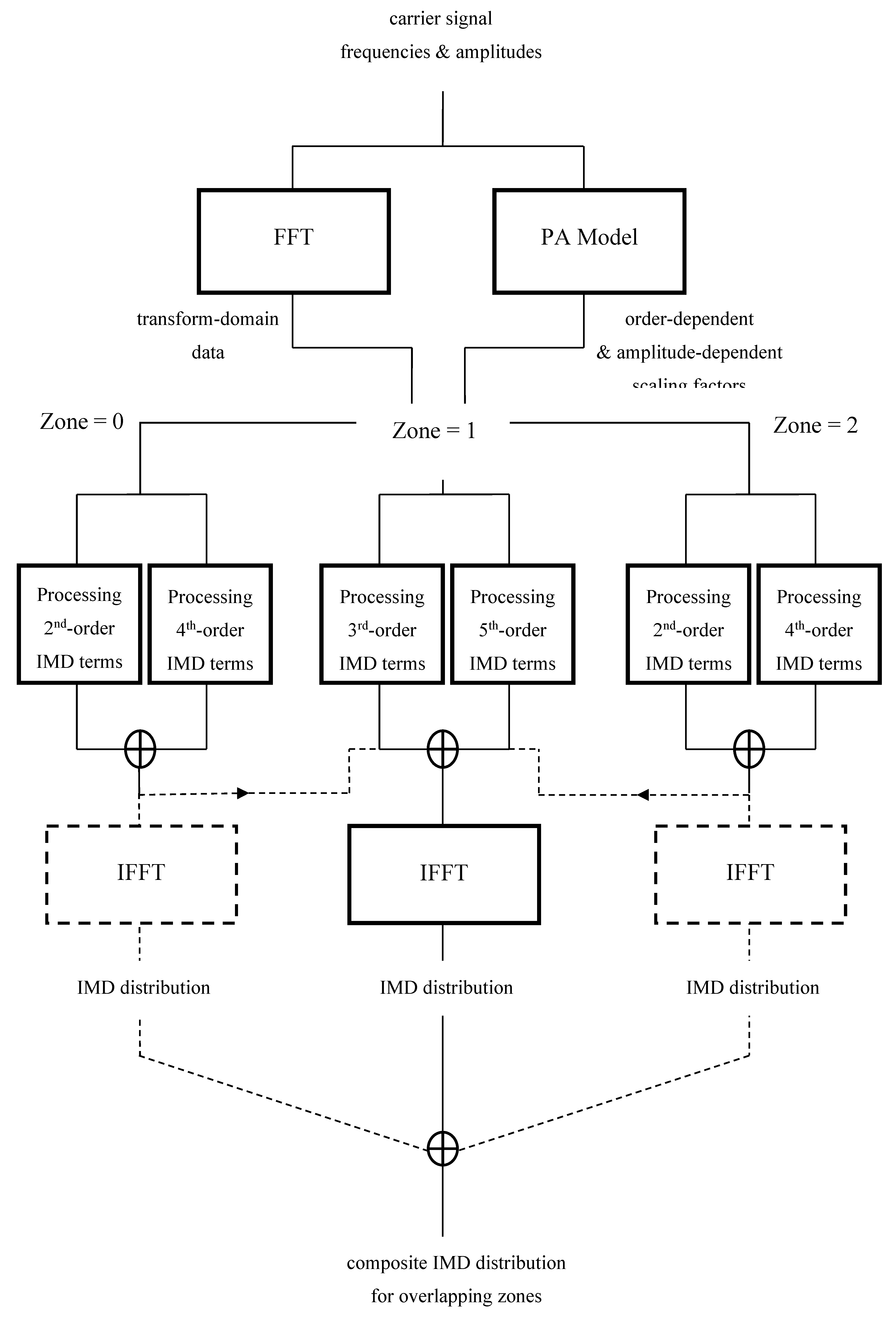
Figure 6.
performance comparison of original and new prediction algorithms for 2nd-order IMD residing in second zone of distortion.
Figure 6.
performance comparison of original and new prediction algorithms for 2nd-order IMD residing in second zone of distortion.
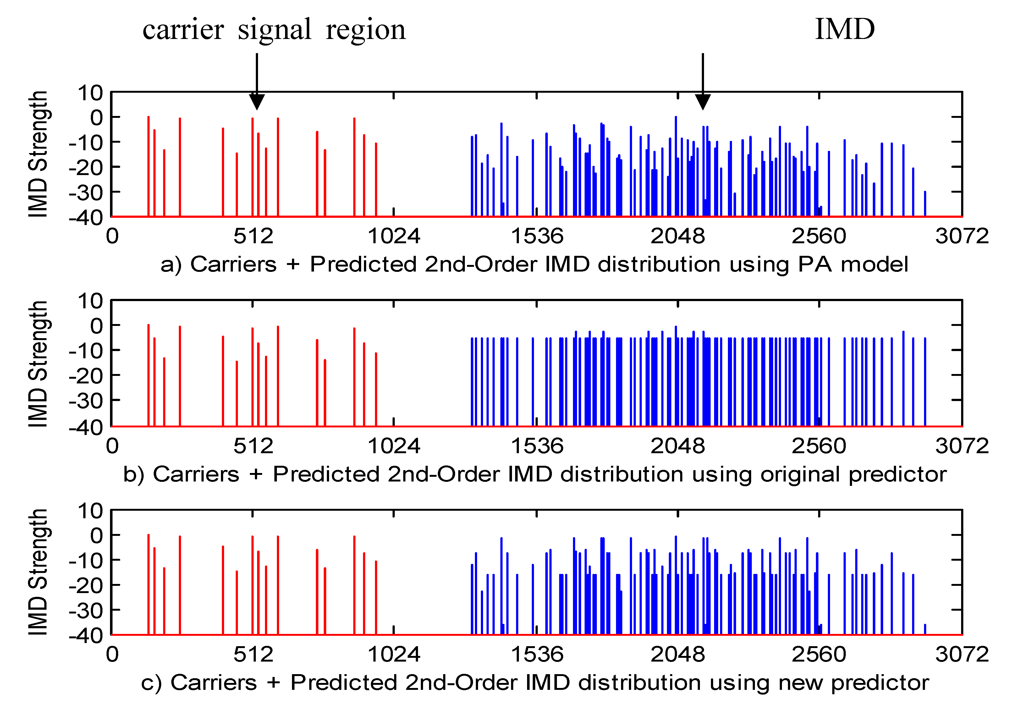

Table 1.
– performance comparison of original and new channel clearance algorithms.
| Iteration No | Measured IMD for Original IMD Prediction & Channel Clearance Scheme: Orders: 2 to 5 Zones: 0 to 5 |
Measured IMD for New IMD Prediction & Channel Clearance Scheme: Orders: 2 to 5 Zones: 0 to 5 |
|---|---|---|
| start = 0 | 0.95 (0 dB) | 0.94 (0 dB) |
| 1 | 0.89 (-0.3 dB) | 0.31 (-4.8 dB) |
| 2 | 0.83 (-0.6 dB) | 0.26 (-5.6 dB) |
| 3 | 0.77 (-0.9 dB) | 0.21 (-6.5 dB) |
| 4 | 0.71 (-1.3 dB) | 0.19 (-6.9 dB) |
| 5 | 0.66 (-1.6 dB) | 0.15 (-8.0 dB) |
| 6 | 0.62 (-1.9 dB) | 0.12 (-8.9 dB) |
| 7 | 0.57 (-2.2 dB) | 0.09 (-10.2 dB) |
| 8 | 0.53 (-2.5 dB) | 0.08 (-10.7 dB) |
Disclaimer/Publisher’s Note: The statements, opinions and data contained in all publications are solely those of the individual author(s) and contributor(s) and not of MDPI and/or the editor(s). MDPI and/or the editor(s) disclaim responsibility for any injury to people or property resulting from any ideas, methods, instructions or products referred to in the content. |
© 2025 by the authors. Licensee MDPI, Basel, Switzerland. This article is an open access article distributed under the terms and conditions of the Creative Commons Attribution (CC BY) license (http://creativecommons.org/licenses/by/4.0/).
Copyright: This open access article is published under a Creative Commons CC BY 4.0 license, which permit the free download, distribution, and reuse, provided that the author and preprint are cited in any reuse.


