Submitted:
13 August 2025
Posted:
14 August 2025
You are already at the latest version
Abstract
An Adaptive Neuro-Fuzzy Inference System (ANFIS) framework for paediatric wrist injury classification (fracture versus sprain) was developed utilising infrared thermography (IRT). ANFIS combines artificial neural network (ANN) learning with interpretable fuzzy rules, mitigating the “black-box” limitation of conventional ANNs through explicit membership functions and Takagi-Sugeno rule consequents. Fourteen children (19 fractures, 21 sprains, confirmed by x-ray radiograph) provided thermal image sequences from which three statistically discriminative temperature distribution features namely standard deviation, inter-quartile range (IQR) and kurtosis were selected. A five-layer Sugeno ANFIS with Gaussian membership functions were trained using a hybrid least-squares/gradient descent optimisation and evaluated under three premise-parameter initialisation strategies: random seeding, K-means clustering, and fuzzy C-means (FCM) data partitioning. Five-fold cross-validation guided the selection of membership functions standard deviation (σ) and rule count, yielding an optimal nine-rule model (σ = 0.1). Comparative experiments show K-means initialisation achieved the best balance between convergence speed (about 48 s for 4000 epochs) and generalisation (validation MSE=0.105; AUC=0.87) versus slower but highly precise random initialisation (AUC=1.00) and rapidly convergent yet unstable FCM (AUC=0.66). The proposed K-means–driven ANFIS offered data-efficient decision support, highlighting the potential of thermal feature fusion with neuro-fuzzy modelling to reduce unnecessary radiographs in emergency bone fracture triage.
Keywords:
artificial neural network
; medical image analysis
; ANFIS
; explainable AI
1. Introduction
Adaptive Neuro-Fuzzy Inference Systems (ANFIS) represent a powerful fusion of two prominent artificial intelligence paradigms namely fuzzy logic and artificial neural networks (ANNs). It is a supervised learning technique integrating the adaptive learning capabilities of ANNs with the human-interpretable rule-based reasoning of fuzzy logic [1]. By adapting the ability of ANNs to learn complex nonlinear mappings from data with the interpretable, rule-based reasoning of fuzzy inference, an ANFIS provides a transparent decision support mechanism. As with a conventional neural network (CNN), an ANFIS is trained using representative datasets. During its learning phase, its network parameters are updated to minimise prediction error on a training data set. Once trained, the ANFIS model structure which comprises both antecedent (fuzzy membership) parameters and consequent (linear output) coefficients is evaluated on previously unseen test data [2]. Low errors on this validation set confirm that the ANFIS architecture is well-suited to the problem being analysed. A notable criticism of standard ANNs is their “black-box” nature, i.e., their learned connection weights do not readily translate into human-understandable rules. ANFIS overcomes this limitation by embedding a fuzzy inference system (FIS) within the network framework. Each neuron corresponds to a fuzzy rule (“IF – THEN” statement), and its parameters can be interpreted as linguistic thresholds. As a result, once training is complete, the entire model can be expressed as a compact set of fuzzy rules which can facilitate knowledge extraction, validation, and expert refinement [3].
Technically, ANFIS models adapt a Sugeno-type fuzzy inference model via an adaptive network of nodes and weighted links. Training proceeds in two intertwined phases employing a hybrid algorithm. During the forward phase, given fixed premise (membership) parameters, consequent coefficients are determined by least-squares estimation to best fit the data [4]. In the backward phase, the resulting error gradients propagate back through the network, and the premise parameters (defining each Gaussian or bell-shaped membership function) are tuned via gradient descent algorithm [5,6]. By decomposing the optimization into these two complementary steps, an ANFIS reduces the dimensionality of the search space compared to pure back-propagation, yielding faster convergence and more stable parameter estimates.
1.1. ANFIS Model Development for Fracture Prediction
The contribution of this article is development and evaluation of an NFIS framework, successfully applied to distinguish between wrist fractures and non-fracture injuries (referred to as sprains in this article) based on IRT images. One of ANFIS’s primary benefits lies in its hybrid architecture: its ANN component automatically adjusts the weights during training to minimise prediction error, while the fuzzy logic component establishes a set of membership functions and corresponding fuzzy rules that capture expert knowledge about how the wrist temperature patterns relate to injury outcomes (i.e., fracture or sprain). This dual mechanism allows the model to learn complex, nonlinear relationships from data while retaining a transparent rule structure. As a result, an ANFIS can achieve an efficient training combined with improved generalisation to new cases. By marrying gradient-based optimisation with linguistic, rule-based inference, ANFIS delivers a robust performance on challenging diagnostic tasks such as thermal image-based fracture detection.
In the following section the related literature is reviewed, the approach to develop and evaluate the ANFIS is explained, and the studies’ findings are discussed.
2. Related Studies
Automated diagnostic platforms are increasingly utilised across diverse types of medical data, ranging from physiological signals to imaging [7,8,9,10]. ANFIS has been successfully employed in numerous medical related applications where medical signals and images serve as the primary inputs to the decision models. Typical examples include detection and diagnosis of diabetes, blood pH imbalances, valvular and rheumatic heart conditions, epileptic seizures, prostate malignancies, and various cancers (colon, leukaemia, lymphoma) via microarray data. ANFIS has also been applied to ophthalmic and optic nerve disorders, analysis of Doppler ultrasound signals (including internal carotid assessments), interpretation of electroencephalogram (EEG) recordings, and identification of arterial abnormalities in the eye. These studies collectively demonstrated the versatility and effectiveness of ANFIS in medical decision-support systems [11,12,13]. ANFIS models were widely used in literature for classification of medical images mainly due to its fast convergence and effective classification abilities even with smaller datasets. For example, the study by Hemanth and colleagues [14] applied an ANFIS to classify four types of abnormal magnetic resonance imaging brain-tumour images which included metastases, meningioma, glioma, and astrocytoma, using six texture features derived from grey-level co-occurrence matrices. Each input feature was fuzzified with two generalised bell-shaped membership functions, yielding 64 fuzzy IF-THEN rules. The model’s training combined least-squares estimation (for rule consequents) with gradient-descent tuning (for membership parameters) over 200 iterations. On a 460-image dataset (120 training, 340 testing), ANFIS achieved an overall classification accuracy of 93.3% which was higher than a fuzzy-nearest-centre classifier (88.6%) and a back-propagation neural network (85.7%). Moreover, the ANFIS model converged in just 1,540 CPU cycles, roughly one-tenth the time required by the other methods, while producing low mean-square errors (training ≈ 0.001, testing ≈ 0.15). Kumar and colleagues [15] presented an ANFIS-based approach to predict COVID-19 epidemic peaks and infection counts in India. They combined nationwide case data sourced from cloud repositories with local demographic and health indicators which includes population density, age distribution, comorbidities, and infrastructure metrics, to construct a two-input, single-output Sugeno model. Using nine trapezoidal membership functions per input and 81 fuzzy rules, the model was trained via a hybrid least-squares and gradient-descent algorithm. Validation against unseen data yielded a low mean square error (MSE = 1.184 × 10⁻³) and an overall predictive accuracy of 86%, outperforming linear and multiple-regression baselines (≈ 83%) both in accuracy and computational efficiency (438 s versus 540–720 s). A hybrid ANFIS framework optimized by Adam and Particle Swarm Optimization (PSO) was proposed to improve Parkinson’s disease (PD) diagnosis accuracy [16]. Using a public UCI dataset of 756 voice recordings (755 features), they first employed an Extra Trees ensemble to select the top five predictive features. Two ANFIS models were then trained separately: one with Adam (gradient-based) and one with PSO (swarm-based) optimizers. The PSO-tuned ANFIS achieved lower training loss and higher precision, while the Adam-tuned model yielded superior accuracy, F1-score, and recall. Across varying epochs, membership functions, and PSO particle counts, both models converged efficiently, with PSO requiring fewer iterations but Adam delivering slightly faster convergence. The best configuration (1000 epochs, 50 particles, four rules per feature) produced test accuracies above 84%, precision up to 91%, and F1-scores near 84%.
Studies have developed artificial intelligence techniques applied to infrared thermal (IRT) images to screen wrist fracture. For example, Shobayo et al. [17] developed and evaluated a convolutional neural network (CNN) to distinguish paediatric wrist fractures from sprains using infrared thermal (IRT) images. The data for each participant were fast Fourier transformed magnitude spectra of the wrist infrared thermal images. These images were recorded from 19 participants with wrist fracture and 21 participants with wrist sprain (i.e., wrist injury did not result in bone fracture). The confirmation of the diagnosis was by x-ray radiography. The image augmentation was employed to minimise over fitting during the training of the CNN. The CNN model achieved 88% sensitivity and 76% overall accuracy (AUC = 0.82). The same authors [18] also used a multilayer perceptron (MLP) model with the same dataset to predict wrist fracture. The optimized MLP achieved a mean sensitivity of 84.2% and specificity of 71.4%, with overall accuracy of 77.5%. The results obtained demonstrated that IRT imaging analysed by MLP can distinguish fractures from sprains, potentially reducing unnecessary x-rays in emergency settings. The authors suggest further validation with larger cohorts, adult patients, and other fracture types.
The literature also demonstrate that ANFIS can effectively leverages both neural learning and fuzzy interpretability to deliver rapid, accurate tumour classification in MRI imaging [14], has the capacity to deliver timely, interpretable guidance for public-health policy and sustainable strategic resource allocation and planning [11,12,13], and when combined with adaptive optimizers, it can produce a better interpretable strategy for early PD detection in clinical settings [16]. Other studies that have used ANFIS for the classification of medical images is presented in the Table 1 below.
This article develops an ANFIS for the first time to interpret IRT images for paediatric wrist fracture screening. The medical diagnosis transparency in decision making provides confidence and traceability. As the decision making by ANFIS is based on a set of rules encapsulating the associated knowledge, the approach adapts explainability. Furthermore, unlike deep learning approaches like CNN that require their extensive parameters to be decided or tuned, ANFIS relies on a much smaller set of operational parameters reducing the possibility of overfitting and speeding up the learning process.
3. Materials and Methods
3.1. Data Collection
The dataset used in this work were taken from children with admissions to a paediatric emergency department (ED) requiring x-ray radiography to determine whether their wrist injury had resulted in a fracture. The study included forty participants, 24 males and 16 females, mean age 10.50 years (standard deviation 2.63 years), of whom 19 had a wrist fracture and 21 had a sprain. The diagnosis was confirmed by x-ray radiography. Thirty participants had analgesic medication, mainly paracetamol and ibuprofen. The participants’ mean body temperature was 36.3 oC (standard deviation 0.4oC). The study recruitment, IRT imaging, ROI selection and statistical representation of the subjects’ images has been previously discussed [18,28]. The study had UK National Health Service Research Ethics Committee approval (identification number: 253940, approval date: 7 March 2019). All participants consented to take part voluntarily.
3.2. ANFIS Model Development
Most ANFIS implementations, regardless of their specific application, share a common five-layer architecture [29]. In this study, we adopted this standard five-layer configuration shown in Figure 1 to leverage its ability to blend human-readable fuzzy rules with adaptive neural learning. Each ANFIS layer performs a distinct operation guided by its learning and data processing algorithm described in the next section.
3.2.1. Layer 1: Fuzzification (Premise Parameters) Layer
The first layer accepts crisp raw inputs (xi, numerical values) representing the infrared thermal imaging information and fuzzified them by determining their degrees of memberships based on the allocated membership functions (MF). The degrees of memberships vary between o (not a member) to 1 (a full member). In this study, Gaussian MFs were used due to their flexibility in representing the input data. A Gaussian MF is characterised by its centre () and width . These parameters are sometimes referred to as the antecedent or premise parameters, since they define the “IF” side of each fuzzy rule (“IF … THEN …”).
3.2.2. Layer 2: Rule Firing Strength (Product Layer)
The second layer consists of neurons, each corresponding to a fuzzy rule that receives the degrees of memberships layer 1. Each node computes the rule’s firing strength ( by taking the product of its incoming membership grades. Mathematically, for rule with antecedent or premise degrees of memberships , , …… the output is
3.2.3. Layer 3: Weight Normalisation
The third layer normalises these raw firing strengths so that they sum to one, i.e., each normalised weight is expressed as:
By normalising the weights, it is ensured that the subsequent weighted averaging in Layer 5 remains bounded and comparable across different input scenarios.
3.2.4. Layer 4: Rule Consequent (Defuzzification) Layer
This layer implements the consequent part of each fuzzy rule using a TSK (Takagi – Sugeno –Kang) formulation. Each rule has its own linear function
where the coefficients and bias , and bias are the consequent parameters, learned during training. Layer 4 multiplies each rule’s normalised firing strength by its consequent output .
3.2.5. Layer 5: Output Aggregation
Finally, the fifth layer aggregates all rule contributions by summing them,
The outputs ( are the model’s crisp decisions. For this study the outputs are continuous values indicating the likelihood of fracture versus sprain.
The ANFIS architecture in this study was configured to learn from three carefully determined thermal image descriptors, i.e., the standard deviation (Std), the interquartile range (IQR), and the kurtosis of the temperature distribution across each wrist region. These three features were selected because as the temperature difference between an injured wrist and its healthy counter lateral for each subject is measured, Std, IQR, and kurtosis consistently exhibited the largest distinction between the two injury outcomes (i.e., fracture and sprain).
The other statistical measures were examined were maximum temperature, minimum temperature, mean temperature and median temperature. The mode and skewness of the temperature did not provide reliable discrimination between the two types of injuries. Their statistical measures overlapped heavily between injured and uninjured hands, failing to offer a clear indication needed for an accurate classification by the ANFIS model. Therefore, to maximise predictive accuracy and reduce model complexity, the ANFIS input was confined to Std, IQR and kurtosis measures [28].
3.3. Cross Validation
We employed a five-fold cross-validation procedure (K=5) to systematically determine two critical hyperparameters for the ANFIS model: the Gaussian membership function width (σ) and the total number of fuzzy rules. In each of the five splits, the training subset was used to fit the model under a candidate combination of σ and rule count, and the remaining validation fold measured the ANFIS performance. The validation errors across all folds were averaged to determine the optimum values of sigma (σ) and rule-set size. These values yielded the lowest mean squared error (MSE) and best generalisation across the entire dataset. For all experiments, the Gaussian membership functions were used. This membership function type is widely used in the fuzzy systems literature because it provides a smooth, continuous mapping from crisp inputs into the (0,1) fuzzy degree, and it is defined by just two parameters: a central location and the width . This simplicity facilitates both transparent rule interpretation and efficient parameter learning. Although Gaussian membership functions were our primary choice, a variety of alternative functions were possible. These included trapezoidal and triangular functions, which offer piecewise-linear transitions. Others include the generalised bell, sigmoid, and other parametric curves [6].
The ANFIS model was trained for 4,000 epochs, but we also implemented an early-stopping criterion to guard against possible overfitting: once the mean squared error (MSE) on the training set dropped below 0.08, the ANFIS training stopped. This strategy ensured that the model did not continue learning noise once an acceptable error threshold was reached. The IRT images were trained on the first-order Sugeno–Kang ANFIS architecture, which can be viewed as a feedforward artificial neural network whose weights and biases are optimised via gradient-descent. In this context, each fuzzy rule corresponded to a set of membership function parameters in the antecedent layer and a linear function in the consequent layer, all of which were tuned simultaneously during training.
To obtain the most suitable configuration, a grid search was performed over two key hyperparameters. First, we experimented with four different fuzzy rule counts which were: 2, 3, 6, and 9 rules to establish how many rules provided the best trade-off between the model complexity and predictive accuracy. Secondly, three different values were tested for the Gaussian membership function width parameter, : 0.1, 0.2, and 0.3. Each combination of rule count and was evaluated using five-fold cross-validation, with the configuration yielding the lowest average MSE on held-out folds selected as optimal. The combination that resulted in least validation error consisted of nine fuzzy rules paired with a Gaussian membership function width of .
3.4. Data Preparation and ANFIS Training
All input features i.e., standard deviation (Std), interquartile range (IQR), and kurtosis were normalised to a range of 0 to 1. This ensured each feature contributed equally during the ANFIS training and avoided dominance by any single metric. After normalisation, the full dataset was split into two subsets: 80 percent of the samples were used to train the ANFIS model while the remaining 20 percent were used for its and performance evaluation on unseen data. The training proceeded using a plain-vanilla gradient-descent algorithm with the learning rate set to 0.05 and 4,000 epochs. Prior to this, a grid search had identified the best combination of Gaussian membership-function width (σ) and fuzzy-rule count based on cross validation error. Once those optimal hyperparameters were determined, they were fixed and used in the final ANFIS training run. This process ensured that the model not only learned effectively from the normalized three-feature inputs but also leveraged the most appropriate membership-function geometry and rule complexity for accurate fracture versus sprain classification.
In an ANFIS model, the process of inferencing can be understood as a “divide and conquer” strategy applied to an n-dimensional input space. Each fuzzy rule’s antecedent (“IF” clause) effectively partitions that continuous input space into smaller, overlapping regions or clusters. When a new input arrives, its degrees of membership in each of these regions are calculated, and the rule’s consequent (“THEN” clause) computes a local output. Finally, all local outputs are combined, typically via a weighted average based on rule firing strengths to produce a single, global prediction. Thus, the structure and performance of the entire ANFIS depend critically on how the input space has been divided into these fuzzy clusters and how accurately those clusters capture the underlying data distribution.
To optimise the placement of these fuzzy-set centres, a “scatter partitioning” approach originally proposed in [30] was adapted. Rather than simply seeding membership functions at random locations, this method uses a clustering algorithm to discover natural groupings in the training data. In our implementation, each input dimension was partitioned into n clusters, and each cluster centre became the parameter for a corresponding membership function. The total number of fuzzy rules then became exactly the number of clusters raised to the power of the number of inputs, i.e., a direct consequence of taking every possible combination of cluster indices across dimensions.
Experiments were carried out on two distinct clustering techniques for identifying those cluster centres: traditional K-means and fuzzy C-means. K-means yields hard, non-overlapping clusters by assigning each data point to its nearest centre, whereas fuzzy C-means produces a soft partition, allowing each point to belong to multiple clusters with varying degrees of membership. In addition, we compared these data-driven initialisations against a baseline in which Gaussian membership functions were centred at random values. By running three separate experiments i.e., random Gaussian seeds, K-means-derived centres, and fuzzy C-means-derived centres, we were able to evaluate the impact of each initialization strategy on both the speed of convergence during training and the ultimate predictive accuracy on held-out data.
4. Results
In this section the results of the experiment undertaken to the evaluate the ANFIS model to screen for wrist fracture are explained.
4.1. Experiment 1: Generalised Membership Function (Generalised Bell) Based on Random Normal Centre Values
In the initial experiment, the classic ANFIS approach was adopted by initialising each membership function centre (c) with random values drawn from a Generalised bell distribution. During training, these centres, along with the network’s consequent weights were refined through gradient-descent back-propagation learning algorithm to minimise prediction error. At the core of this method is the Gaussian membership function, which translates each crisp input into degrees of memberships using the Gaussian function. The curve’s location along the input axis is determined by the function’s centre, effectively acting as the mean of the Gaussian function. Its spread, or standard deviation, controls how quickly the membership falls off away from the centre. Based on prior cross-validation experiments, this standard deviation was fixed to . By combining randomly initialised centres with a carefully chosen width, it is ensured that the network begins with diverse, well-distributed fuzzy sets and then iteratively adapts both the premise (centres) and consequent parameters to capture complex, nonlinear relationships in the data.
The plot in Figure 2 shows the manner the training (blue) and validation (orange) mean squared error (MSE) steadily decline over the 4,000 epochs when using randomly initialised Gaussian membership functions.
Initially the MSE associated with the ANFIS training declines rapidly then very gradually approach but never quite reaching the red target line at 0.08 for training MSE. The validation curve dips below the training curve around epoch 300, then rises slightly before converging back toward the training error, which indicates some over- and under-shooting as the model settles.
Table 2 quantifies the ANFIS performance every 800 epochs. By epoch 800, training MSE is 0.153 and validation MSE 0.193 (RMSEs 0.392 and 0.439), with a 0.039 difference. By epoch 4,000, errors have further shrunk (training MSE = 0.130, validation MSE = 0.151) and the MSE difference narrows to 0.021. RMSE follows the same downward trend. Elapsed time grows linearly at about 39 s per 800 epochs, totalling roughly 194 s at 4,000 epochs.
The confusion matrix in Figure 3 summarises the ANFIS model’s performance on the validation set. The rows represent the true labels (“No Fracture or sprain” and “Fracture”), while the columns show the model’s predicted labels.
- True Negatives (number of sprain cases correctly predicted): 5 from 5 cases.
- False Positives (number of sprain cases detected as fracture): 0 from 5 cases.
- False Negatives (number of fracture cases detected as sprain): 1 from 3 cases.
- True Positives (number of fracture cases detected as fracture): 2 from 3 cases.
Out of eight cases, the model correctly identified seven (5 non-fractures and 2 fractures) and missed one fracture. This indicates high specificity (no sprain cases misclassified) and a small false-negative rate, suggesting the model reliably detected sprains but with the current small data set for its training it can occasionally overlook actual fractures.
The Area Under Curve (AUC)- Receiver Operating Characteristic (ROC) curve and the contour plot are shown in Figure 4a and 4b respectively. The AUC-ROC curve evaluates the ANFIS model’s ability to distinguish fractures from sprain (non-fractures) cases on the validation set. The true positive rate is plotted against the false positive rate at various classification thresholds. The orange ROC line appears on the top and left axes, indicating that the model achieves 100% sensitivity with 0% false positives across thresholds which is set at 0.5. The dashed diagonal represents a random classifier (AUC = 0.5). Here, the model’s Area Under the Curve (AUC) is 1, signifying perfect discrimination every fracture is detected with no healthy wrists falsely flagged.
The contour plot in Figure 4b visualises the trained ANFIS model’s continuous output (“Predicted Score”) over the 2-D plane of standard (Std, x-axis) and Kurtosis (y-axis), with IQR held fixed at its median value which is approximately 0.16. We have chosen to fix the IQR feature since we have a three-feature model, which will in turn provide a 3-D mapping. Fixing the IQR at the median value helps to slice the dimensional viewing of the contour plot in 2-D. The IQR feature was also selected for fixing as it provides the least variations between datapoints from all the 39 subjects used for this study. Selecting the median value provides the best representation of the contour plot prediction for the fracture and non-fracture (sprain) validation dataset. Moving this value up or down changes the shape and position of the yellow and blue regions which in turns places the validation dataset in the wrong contour. The colour scale in the plot shows the predicted score and the colour bar on the right maps the model’s real-valued output where:
- Yellow/green regions with scores , indicates stronger “fracture” predictions.
- Blue/purple regions with scores indicates stronger “no-fracture” (sprain) predictions.
The standard deviation feature (Std) of the infrared thermal image varies from 0 (left) to 1 (right) on the x-axis, i.e., the Kurtosis feature varies from 0 (bottom) to 1 (top) on the y-axis. Every pixel in the plot is a synthetic point, represented by the selected features from the thermal images as evaluated by the ANFIS model. On the overlaid validation samples, the red dots represent the true fracture cases where on the validation dataset. The blue dots are the true non-fracture (sprain) cases in which validation dataset are presented as . Where the background colour shifts toward yellow/green, the model’s score is higher, and these are the regions where the model will correctly classify as fracture (threshold is 0.5). Conversely, deep blues and purples are areas the model considers “no fracture” (sprain). One of the red dots, representing the fracture case appeared in the bluish zone and this is the only misclassified case from the validation data. The rest of the red dots (fracture cases) lied in the green/yellow areas, representing the correctly predicted fracture cases. The smooth contour lines show the manner the model interpolates between its learned fuzzy rules. Whenever it peaks, (where there is a bright yellow bump), this corresponds to combinations of Std and Kurtosis where your model is most effective for fracture prediction. The valleys (areas representing dark purple troughs) are regions of strong confidence in “no fracture” (sprain) prediction.
4.2. Experiment 2: Centre Value Based on K Means Clustering for the Generalised Membership Function
For experiment 2, K-means clustering was used to determine the number of clusters for the input data. K-means iteratively assigns each data point to its nearest cluster and then recomputes each centre as the mean of its assigned points. After convergence, the coordinates of the cluster centroids are stored and sorted so that the membership functions are ascend in the order of their centre location. To ensure that there is a reasonable spread in each Gaussian, we computed the minimum difference between neighbouring centres and set each sigma () of the Gaussian membership function to half the difference. This process ensured the adjacent Gaussian membership functions just touch about 0.61 of their peaks, thereby providing a good coverage without an excessive overlap. During the ANFIS forward pass, each input was converted to its associated degrees of memberships, effectively creating a data driven, well-spaced Gaussian MFs. By initialising the MFs via K-means rather than randomly, the membership functions were aligned with actual clusters in the data.
Table 3 quantifies error and timing every 800 epochs as in experiment 1. By epoch 800, the training MSE is 0.117 and validation MSE 0.106 (with validation outperforming training, ΔMSE = –0.011). RMSEs mirror these trends (0.341 vs. 0.325). Further snapshots show the MSEs oscillate slightly but stay within 0.10-0.15 for both sets, and the ΔMSE remains negative, indicating the model generalizes slightly better than it fits the training data. Elapsed time grows linearly at roughly 9.6 s per 800 epochs, totalling about 48 s at 4,000.
The plot in Figure 5 shows the training (blue) and validation (orange) MSE over 4,000 epochs after initializing the Gaussian MF centres via the K-means algorithm. Both curves drop sharply within the first 200 epochs, reaching low MSE values near the 0.08 target. However, the validation curve then exhibits jagged fluctuations, especially between 1,000 and 2,500 epochs before settling again toward the baseline. The training curve remains relatively smooth.
Figure 6 shows the confusion matrix for the K-means initialised ANFIS model on the validation set. Rows show the true class (“No Fracture or sprain” on top, “Fracture” below) and columns show the predicted classes. Out of 5 true non-fracture cases, the model correctly labelled 4 cases and misclassified 1 case as fracture (false positive). Of 3 true fracture cases, it correctly identified 2 cases (true positives) but misses 1 case (false negative). In total, 6 of 8 cases are classified correctly, yielding an overall accuracy of 75%. The false-positive and false-negative counts also allows computation of a specificity of 80% and sensitivity of 67%.
Figure 7a shows the ROC curve of the K-means initialised ANFIS. The orange curve rises quickly, where sensitivity jumps to 0.67 with zero false positives, then reaches 1.0 at false positive rate (FPR) = 0.5 before flattening at the top right. The AUC is 0.867, which indicates the model’s effectiveness.
Figure 7b visualises the K-means initialised ANFIS model’s continuous output over the 2-D plane of Std (x-axis) and Kurtosis (y-axis), with IQR fixed at its median value , with each background colour representing the model’s predicted score. Ideally, most red dots which represents the fracture cases lie in yellow regions (correctly predicted), while blue dots (sprain) fall into cooler areas. Here, a few misclassifications have occurred where the points crossed those abrupt rule boundaries, highlighting the areas where the model’s partitioning could be further refined or smoothed.
4.3. Experiment 3: Centre Value Based on Fuzzy c-Means Clustering for the Generalised Membership Function
For experiment 3, fuzzy c-means (FCM) clustering was used to place the gaussian membership function centre based the spatial dimension of the input data. For each input feature set, i.e., (sd, Kurtosis and IQR), a vector of observed values was prepared from the training data and reshaped to fit the fuzzy function parameters. The c-mean’s fuzzification exponent value was set to 3. This value was chosen to suitably soften the cluster boundaries. FCM updates the degrees of membership values () for each iteration up to the maximum iteration value ( ) or whether the change in centre falls below a small error value set at . The centre value obtained for every iteration is then sorted from lowest to highest to represent the Gaussian membership centre of the input. To ensure the Gaussian membership functions cover the input range without excessive overlap, the difference between the adjacent centres were computed such that each width was set equal to half the smallest centre-to-centre gap, so the neighbouring Gaussians meet at of their peaks. During prediction, each input value was converted into a degree of membership value utilising the gaussian membership function, ensuring that the membership functions were anchored to the actual data clusters rather than some arbitrary points.
Figure 8 shows the manner the MSE evolved when the Gaussian membership function centres were initialised by fuzzy c-means. Both curves drop sharply in the first 50-100 epochs. The training MSE then stabilises around 0.19, with only minor ripples, while the validation MSE initially peaks near 0.75, then steadily declines to about 0.17 by epoch 4,000 eventually crossing below the training curve.
Table 4 quantifies these same trends at 800-epoch intervals. At epoch 800, training MSE is 0.189 and validation MSE 0.715 . By epoch 2,400, validation error has fallen to 0.521, closing the gap. By epoch 4,000 both errors converge (training = 0.171, validation = 0.167; . RMSE values mirror this pattern (training , validation dropping from to ). The total training time is significantly low at only 6 s for 4,000 epochs.
Figure 9 shows the confusion matrix for the FCM-initialised ANFIS on the validation set. Out of five true non-fracture cases, four were correctly identified (true negatives) and one is misclassified as fracture (false positive). Out of three true fractures, only one was correctly detected (true positive) while two were missed (false negatives). This performance yields an overall accuracy of 62.5%, specificity of 80%, and sensitivity of 33%.
The Figure 10a is ROC curve for the FCM-initialised ANFIS, showing how sensitivity varies with the false-positive rate as the classification threshold shifts. The orange-coloured curve initially increases to 0.33 true positive rate at zero false positives, then to 0.67 at false positive rate (FPR) = 0.4, and finally reaches 1.0 at FPR = 1.0. The resulting AUC of 0.667 indicating a modest discriminative power: the model is better than chance but still struggles to reliably distinguish fractures from non-fractures under this FCM initialisation. Figure 10b shows the FCM-initialised ANFIS decision surface over two features i.e., Std (x-axis) and Kurtosis (y-axis), with IQR fixed at 0.16. Ideally, red points lie in yellow regions and blue in purple. Here, most red dots fall in positive (yellow/green) zones, but one lies in (blue/purple) region, showing a misclassification. The irregular contours highlight the manner FCM-initialized Gaussian membership functions partition the feature space for fracture detection.
5. Discussion
Across the three experiments, there was a clear trade-off between the convergence speed, generalisation and classification accuracy. Experiment 1 (random centres) achieved steady but relatively slow MSE declines, requiring nearly 194s to complete 4000 epochs and settling at a training/validation MSE of 0.1304/0.1514. Its ∆MSE narrowed from 0.039 to 0.021, indicating modest overfitting. Experiment 2 (K-means) converged faster, taking only 48 s for 4000 epochs, with training/validation MSE fluctuating around 0.14/0.10 and ∆MSE remaining slightly negative (-0.011 to -0.041), showing slight underfitting but excellent stability. Experiment 3 (FCM) was fastest (6 s for 4000 epochs) but exhibited unstable validation error, initially peaking near 0.75 before gradually falling to 0.167, finally matching training MSE at 0.171 (∆MSE ≈ –0.004). The dramatic early spikes in Experiment 3 suggest poor initial cluster placement.
Experiment 1 delivered highest specificity and perfect precision i.e., Accuracy 0.88, Precision=1.00, Recall=0.67, F1=0.80 (which combines Precision and Recall to a single value), AUC=1.00, thus reflecting near-ideal separation on the small validation set. Experiment 2 traded precision for broader generalisation (accuracy=0.75, precision=0.67, recall=0.67, F1=0.67, AUC=0.87), yet provided the most balanced sensitivity and specificity outcomes. For Experiment 3, the late-stage validation improvements were insufficient to overcome early misclassifications (accuracy=0.63, precision=0.50, recall= 0.33, F1=0.40, AUC=0.67), indicating that its soft clustering induced ambiguous rule boundaries.
Random initialization (Experiment 1) can achieve high accuracy but at the expense of longer training time and slight overfitting. K-means (Experiment 2) strikes the best balance: it leverages data-driven cluster placement to accelerate convergence, reduce overfitting, and yield robust, reproducible results. FCM (Experiment 3) offers the quickest training but suffers from early instability and poor discrimination, likely because its fuzzy assignments blur crucial rule partitions. Overall, K-means–driven ANFIS emerges as the most effective strategy, combining computational efficiency with strong and consistent classification performance.
The accuracy of prediction was compared with the literature and Experiment 1 with the generalised bell MF had the highest accuracy when compared with the two papers by Shobayo et al., [17, 18] which used the same dataset as shown in Figure 12. K-means centred cluster was very close in terms of accuracy but proffer faster raining convergence when compared to the models with higher accuracy.
The limitations of this study include a relatively small cohort, which restricted external validity; additional multi-centre data and inclusion of varied fracture patterns are needed to solidify performance estimates and refine rule universality. Future work will explore adaptive membership evolution (e.g., regularised shape constraints) and ensemble neuro-fuzzy architectures, to further boost sensitivity without sacrificing interpretability. In summary, the K-means initialised ANFIS provided a transparent, data-efficient and clinically promising adjunct for paediatric wrist fracture triage, illustrating the manner principled neuro-fuzzy design can unlock value in emerging thermographic biomarkers while maintaining trust and explainability in frontline decision support.
6. Conclusions
This study demonstrated that ANFIS can effectively discriminate paediatric wrist fractures from sprains using a compact set of thermographic features (standard deviation, inter-quartile range, kurtosis) derived from infrared recordings. By embedding Takagi – Sugeno fuzzy rules within a trainable network, the approach overcomes the opacity of conventional “black-box” classifiers while retaining nonlinear modelling capacity, allowing each learned rule and membership function to be clinically scrutinised and, if needed, refined by domain experts. A central finding was the influence of premise parameter initialisation on both convergence dynamics and generalisation: K-means seeded Gaussian memberships yielded the most favourable balance, which included fast optimisation with stable validation error, surpassing the slower yet high-precision random seeding and the rapid but volatile fuzzy C-means alternative (higher early validation instability, lower AUC). This indicates that data-aware, crisp clustering can establish sufficiently separated initial fuzzy partitions without inducing the excessive overlap that may dilute discriminative rule firing seen in soft clustering schemes. The hybrid least-square and gradient descent training further reduced search space dimensionality, contributing to efficient error minimisation and supporting deployment within time-sensitive emergency workflows.
Author Contributions
Conceptualization, O.S., R.S., S.R.; methodology, O.S., R.S., S.R.; software, O.S., R.S., S.R.; validation, O.S., R.S., S.R.; formal analysis, O.S., R.S, S.R.; investigation, O.S., R.S., S.R.; resources, O.S., R.S., S.R.; data curation, O.S., R.S., S.R.; writing—original draft preparation, O.S., R.S., S.R.; writing—review and editing, O.S., R.S., S.R.; visualization, O.S., R.S., S.R.; supervision, R.S.; project administration, O.S., R.S. All authors have read and agreed to the published version of the manuscript.
Funding
This research received no external funding.
Institutional Review Board Statement
This study was conducted in accordance with the Declaration of Helsinki and approved by the National Health Service Research Ethics Committee (United Kingdom, identification number: 253940, approval date: 7 March 2019).
Informed Consent Statement
Informed consent was obtained from all subjects involved in this study. None of the participants can be identified in this article.
Data Availability Statement
Patient data are not shared due to ethical restrictions.
Acknowledgments
The authors are grateful to all participants (patients and their carers) who so kindly assisted this work by taking part in the data recordings.
Conflicts of Interest
The authors declare no conflicts of interest.
Abbreviations
The following abbreviations are used in this manuscript:
| MRI | Magnetic Resonance Imaging |
| OCT | Optical Coherence Tomography |
References
- Suparta, W.; Samah, A.A. Rainfall Prediction by Using ANFIS Times Series Technique in South Tangerang, Indonesia. Geodesy and Geodynamics 2020, 11, 411. [Google Scholar] [CrossRef]
- Talpur, N.; Abdulkadir, S.J.; Alhussian, H.; Hasan, M.H.; Aziz, N.; Bamhdi, A. Deep Neuro-Fuzzy System application trends, challenges, and future perspectives: a systematic survey. Artif Intell Rev 2022, 56, 865. [Google Scholar] [CrossRef] [PubMed]
- Kar, S.; Das, S.; Ghosh, P.K. Applications of neuro fuzzy systems: A Brief Review and Future Outline. Applied Soft Computing 2014, 15, 243–259. [Google Scholar] [CrossRef]
- Hamdan, H.; Garibaldi, J.M. In In Adaptive Neuro-Fuzzy inference System (ANFIS) in Modelling Breast Cancer Survival; International Conference on Fuzzy Systems; IEEE: 2010, 1–8.
- Roy, S.S. Design of Adaptive Neuro-Fuzzy Inference System for Predicting Surface Roughness in Turning Operation. Journal of Scientific and Industrial Research 2005, 64, 653. [Google Scholar]
- Saatchi, R. Fuzzy Logic Concepts, Developments and Implementation. Information 2024, 15. [Google Scholar] [CrossRef]
- Shobayo, O.; Saatchi, R. Developments in Deep Learning Artificial Neural Network Techniques for Medical Image Analysis and Interpretation. Diagnostics 2025, 15, 1072. [Google Scholar] [CrossRef]
- Pilehvari, S.; Morgan, Y.; Peng, W. An Analytical Review on the Use of Artificial Intelligence and Machine Learning in Diagnosis, Prediction, and Risk Factor Analysis of Multiple Sclerosis. Mult Scler. Relat. Disord. 1057; 61. [Google Scholar]
- Purwono, P.; Wulandari, A.N.E.; Nisa, K. Explainable Artificial Intelligence (XAI) in Medical Imaging: Techniques, Applications, Challenges, and Future Directions. Advanced Mechanical and Mechatronic Systems 2025, 1, 52–66. [Google Scholar]
- Azeez, O.; Abdulazeez, A. Classification of Brain Tumor based on Machine Learning Algorithms: A Review. Journal of Applied Science and Technology Trends 2025, 6, 1. [Google Scholar] [CrossRef]
- Hosseini, M.S.; Zekri, M. Review of Medical Image Classification Using the Adaptive Neuro-Fuzzy Inference System. Journal of Medical Signals & Sensors.
- Übeyli, E.D. Adaptive Neuro-Fuzzy Inference Systems for Automatic Detection of Breast Cancer. J. Med. Syst. 2009, 33, 353. [Google Scholar] [CrossRef]
- Avci, E.; Turkoglu, I. An Intelligent Diagnosis System Based on Principle Component Analysis and ANFIS for the Heart Valve Diseases. Expert Syst. Appl. 2009, 36, 2873–2878. [Google Scholar] [CrossRef]
- Hemanth, D.J.; Vijila, C.K.S.; Anitha, J. Application of Neuro-Fuzzy Model for MR Brain Tumor Image Classification. International Journal of Biomedical Soft Computing and Human Sciences: the Official Journal of the Biomedical Fuzzy Systems Association.
- Kumar, R.; Al-Turjman, F.; Srinivas, L.; Braveen, M.; Ramakrishnan, J. ANFIS for Prediction of Epidemic Peak and Infected Cases for COVID-19 in India. Neural Computing and Applications 2023, 35, 7207–7220. [Google Scholar] [CrossRef] [PubMed]
- Pasha, A.; Ahmed, S.T.; Painam, R.K.; Mathivanan, S.K.; Mallik, S.; Qin, H. Leveraging ANFIS with Adam and PSO optimizers for Parkinson’s disease. Heliyon 2024, 10. [Google Scholar] [CrossRef] [PubMed]
- Shobayo, O.; Saatchi, R.; Ramlakhan, S. Convolutional Neural Network to Classify Infrared Thermal Images of Fractured Wrists in Pediatrics. Healthcare 2024, 12. [Google Scholar] [CrossRef] [PubMed]
- Shobayo, O.; Saatchi, R.; Ramlakhan, S. Infrared Thermal Imaging and Artificial Neural Networks to Screen for Wrist Fractures in Pediatrics. Technologies 2022, 10. [Google Scholar] [CrossRef]
- Al-Ali, A.; Elharrouss, O.; Qidwai, U.; Al-Maaddeed, S. ANFIS-Net for Automatic Detection of COVID-19. Sci Rep 2021, 11. [Google Scholar] [CrossRef]
- Sharma, M.; Mukharjee, S. Brain Tumor Segmentation using Hybrid Genetic Algorithm and Artificial Neural Network Fuzzy Inference System (ANFIS). IJFLS 2012, 2, 31. [Google Scholar] [CrossRef]
- Birgani, M.T.; Chegeni, N.; Birgani, F.F.; Fatehi, D.; Akbarizadeh, G.; Shams, A. Optimization of Brain Tumor MR image Classification Accuracy using Optimal Threshold, PCA and Training ANFIS with Different Repetitions. Journal of Biomedical Physics & Engineering.
- Chatterjee, S.; Das, A. A Novel Systematic Approach to Diagnose Brain tumor Using Integrated Type-II Fuzzy Logic and ANFIS (Adaptive Neuro-Fuzzy Inference System) Model. Soft Computing-A Fusion of Foundations, Methodologies & Applications.
- Kumarganesh, S.; Suganthi, M. An Enhanced Medical Diagnosis Sustainable System for Brain Tumor Detection and Segmentation using ANFIS Classifier. CMIR 2023, 14, 271. [Google Scholar] [CrossRef]
- Richard, A.B.; Friska, J.; Narayanan, K.L. In Implementation of ANFIS Assisted Modified CNN Classifier for Autism Spectrum Disorder Detection; 2025 International Conference on Visual Analytics and Data Visualization (ICVADV); IEEE: 2025, 1322–1326. [Google Scholar]
- Balakrishnan, N.D.; Perumal, S.K. Monitoring Kidney Microanatomy During Ischemia-Reperfusion using ANFIS Optimized CNN. Int. Urol. Nephrol. 2025, 1–12. [Google Scholar] [CrossRef]
- Mayeta-Revilla, L.; Cavieres, E.P.; Salinas, M.; Mellado, D.; Ponce, S.; Torres Moyano, F.; Chabert, S.; Querales, M.; Sotelo, J.; Salas, R. Radiomics-Driven Neuro-Fuzzy Framework for Rule Generation to Enhance Explainability in MRI-Based Brain Segmentation. Frontiers in Neuroinformatics 2025, 19, 1550432. [Google Scholar] [CrossRef]
- Tiwari, R.G.; Misra, A.; Maheshwari, S.; Gautam, V.; Sharma, P.; Trivedi, N.K. Adaptive Neuro-FUZZY Inference System-Fusion-Deep Belief Network for Brain Tumor Detection using MRI Images with Feature Extraction. Biomedical Signal Processing and Control 2025, 103, 107387. [Google Scholar] [CrossRef]
- Shobayo, O.; Saatchi, R.; Reed, C.; Ramlakhan, S. In Correlation of Skin Temperature with Time Since Injury in Paediatric Wrist Injuries: An Infrared Thermal Image Analysis; 60th Annual Conference of the British Institute of Non-Destructive Testing, NDT 2023; British Institute of Non-Destructive Testing: 2023; 167–177.
- Jang, J. ANFIS: Adaptive-Network-Based Fuzzy Inference System. IEEE Trans. Syst. Man Cybern. 1993, 23, 665–685. [Google Scholar] [CrossRef]
- Yeom, C.; Kwak, K. Performance Comparison of ANFIS Models by Input Space Partitioning Methods. Symmetry 2018, 10. [Google Scholar] [CrossRef]
Figure 1.
An ANFIS architecture of the fracture classification system with three inputs and two outputs.
Figure 1.
An ANFIS architecture of the fracture classification system with three inputs and two outputs.
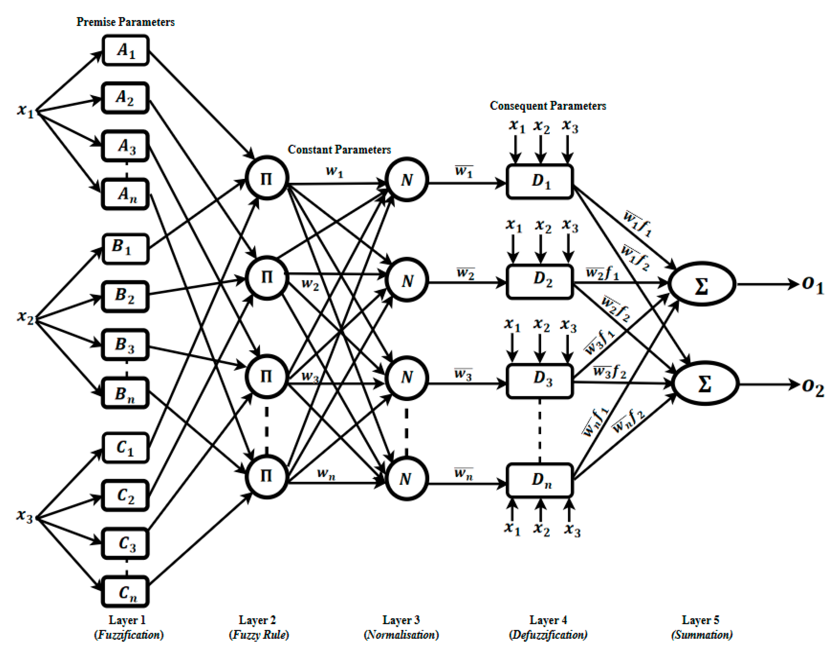
Figure 2.
Training and Validation MSE for Experiment 1.
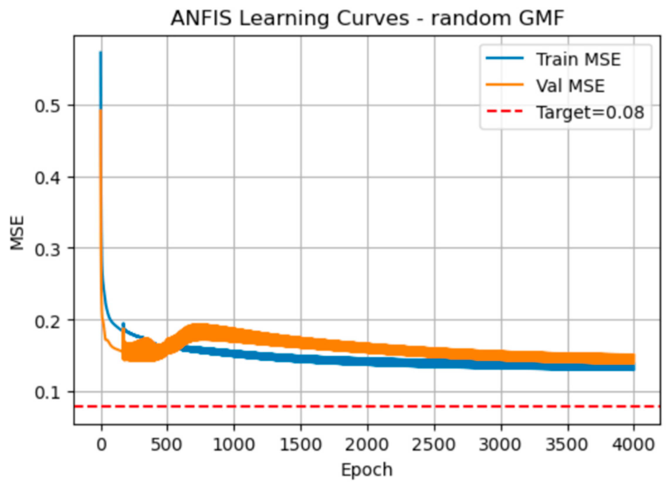
Figure 3.
Confusion Matrix for Experiment 1.
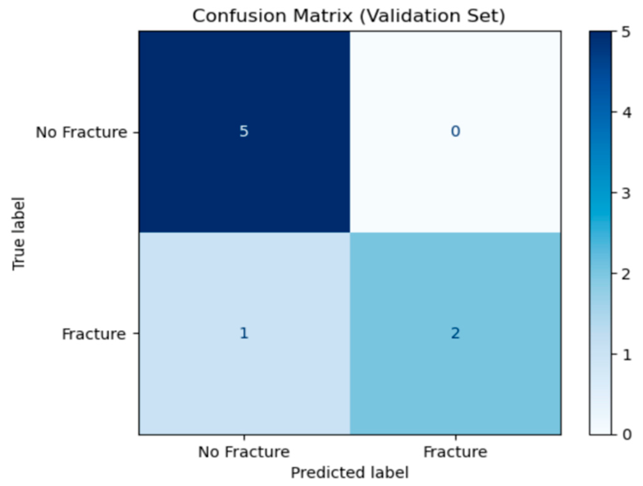
Figure 4.
(a) AUC-ROC for experiment 1, (b) Contour plot of experiment 1.
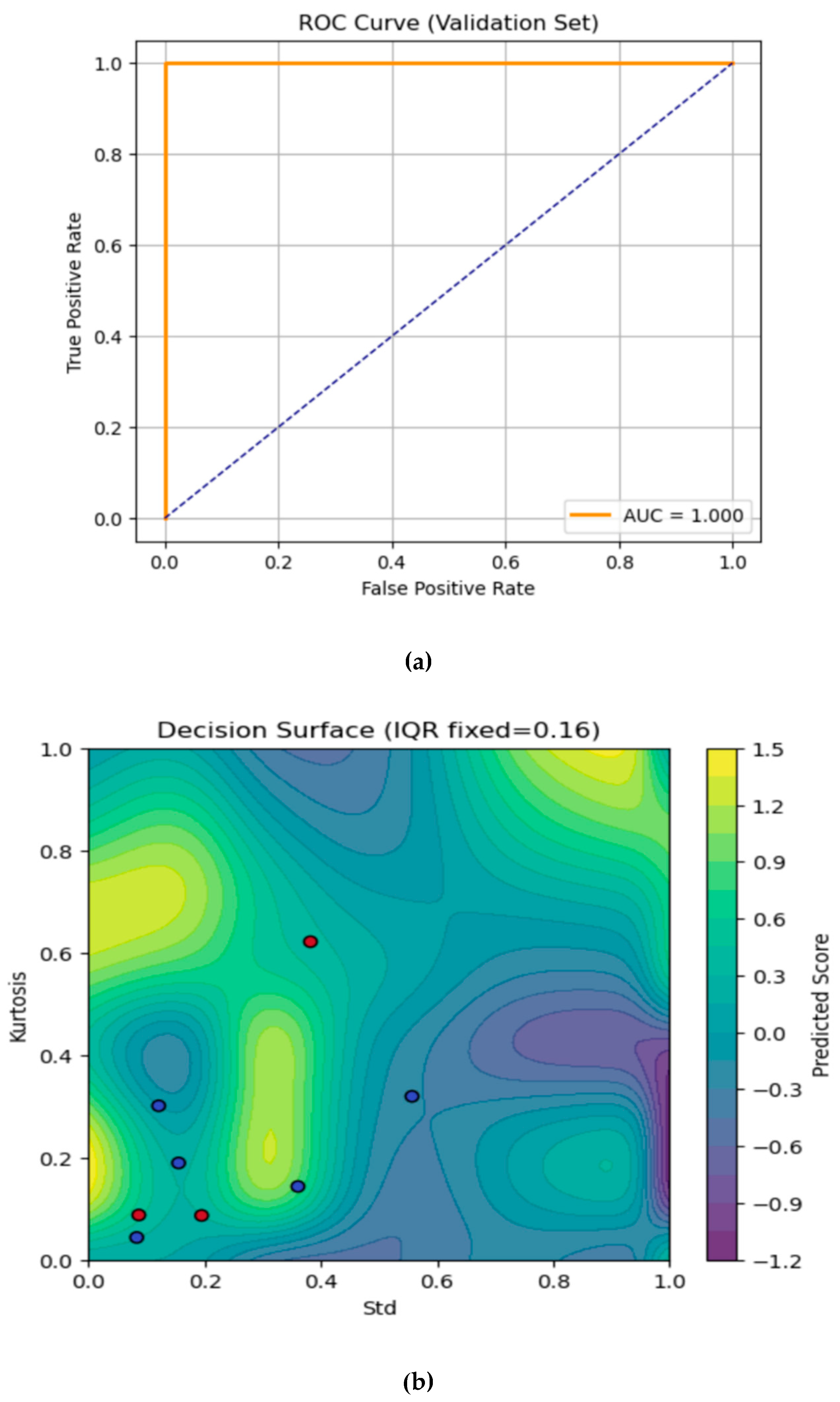
Figure 5.
Training and Validation MSE for Experiment 2.
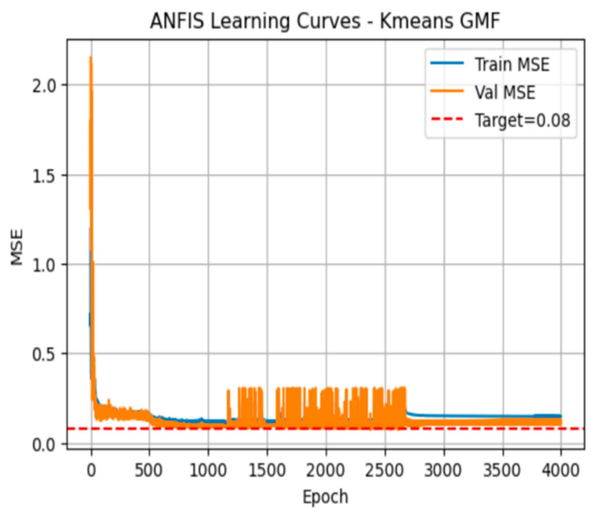
Figure 6.
Confusion matrix for Experiment 2.
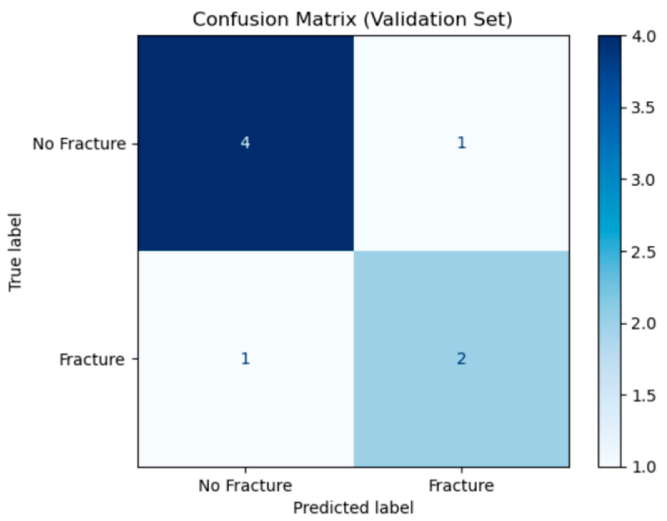
Figure 7.
(a) AUC-ROC for experiment 2, (b) Contour lot of experiment 2.
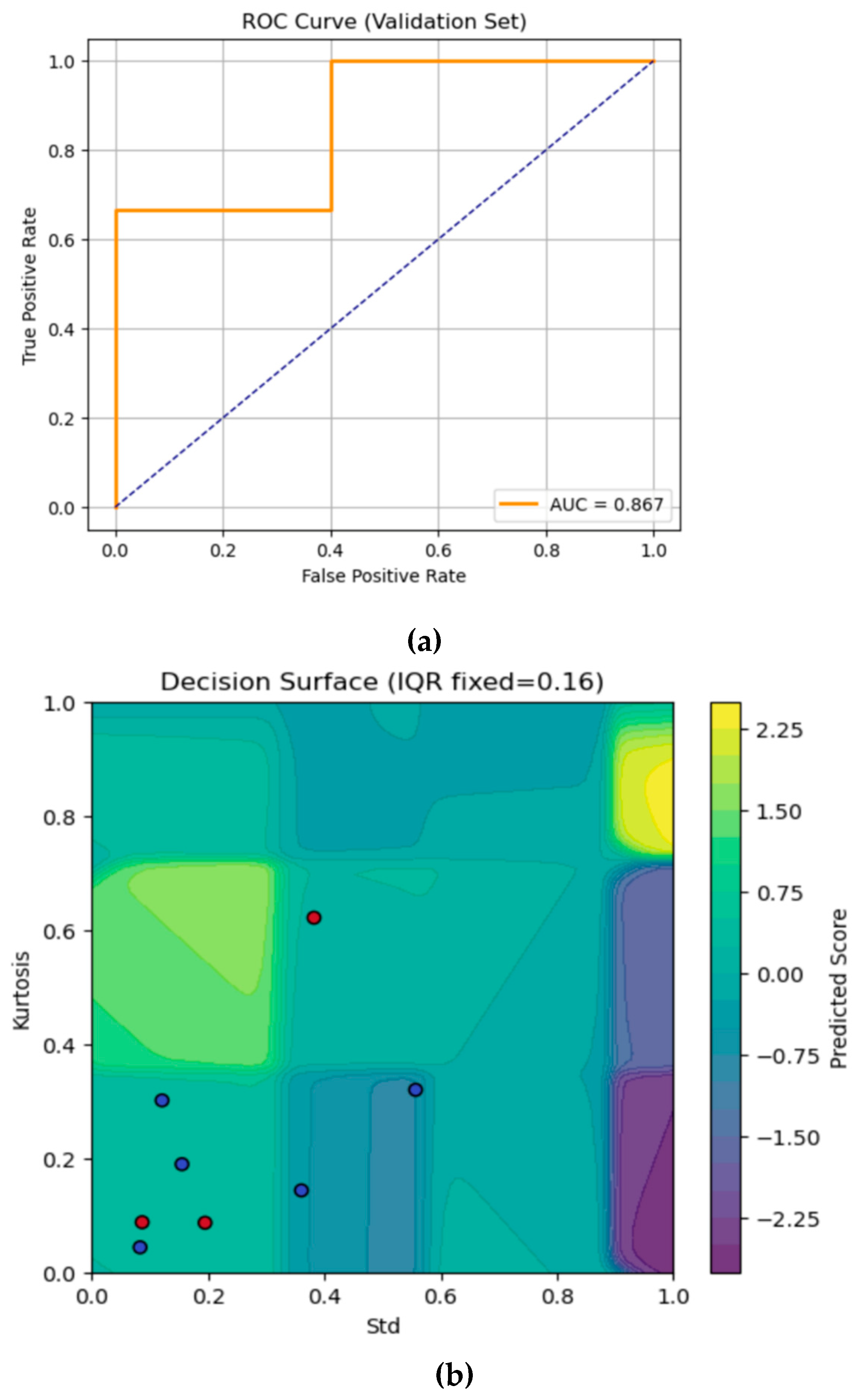
Figure 8.
Training and Validation MSE for Experiment 3.
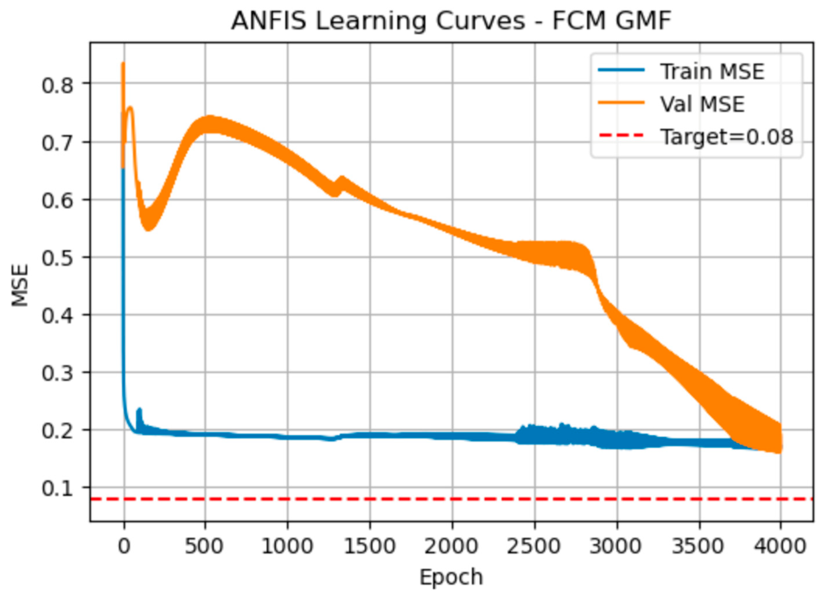
Figure 9.
Confusion matrix for experiment 3.
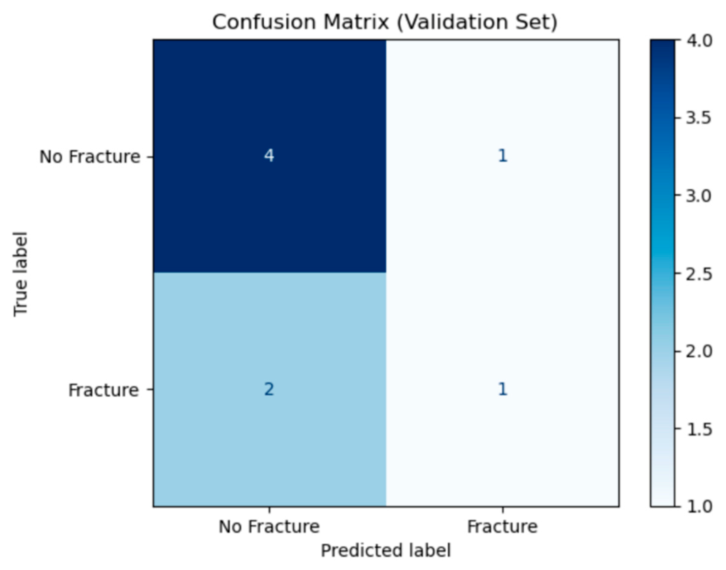
Figure 10.
(a) AUC-ROC for experiment 3 (b) Contour plot of experiment 3.
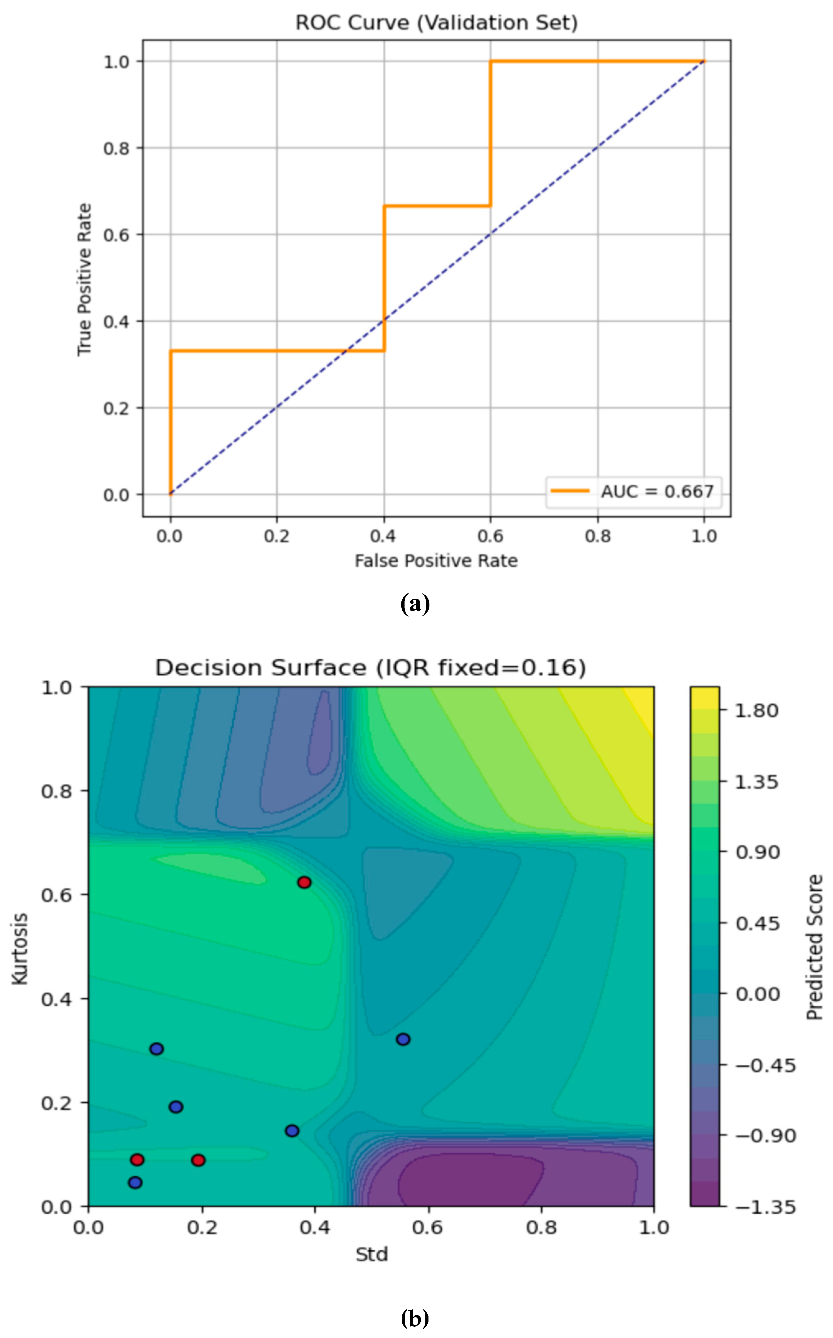
Figure 11.
Evaluation metrics across the experiments.
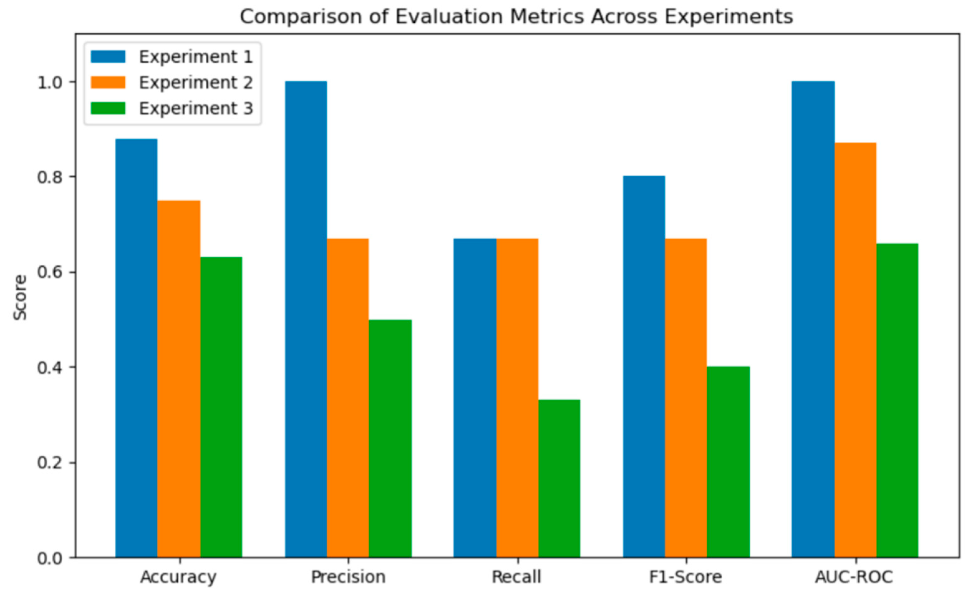
Figure 12.
Accuracy comparison with existing literature.
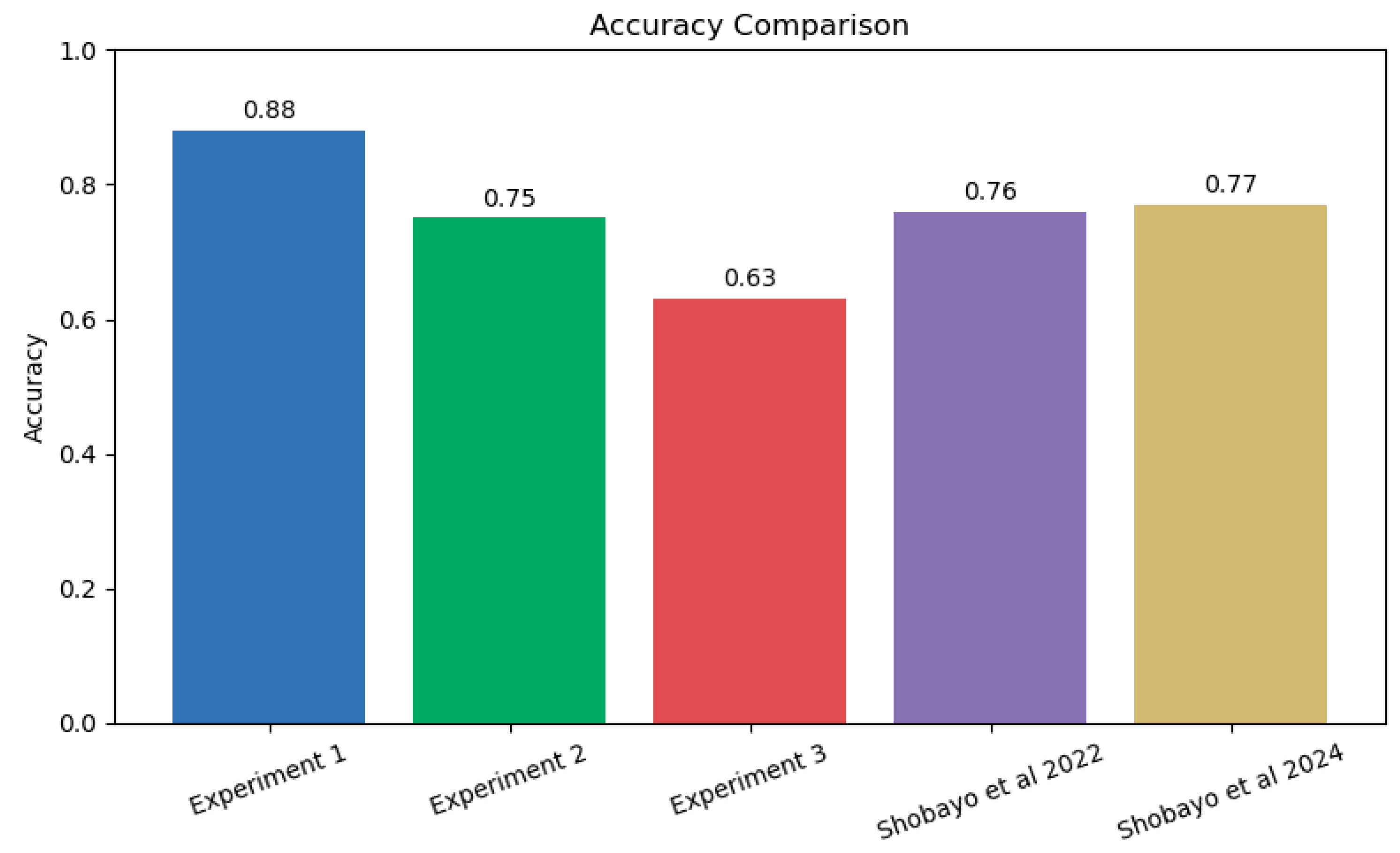

Table 1.
Summary of ANFIS techniques for medical image analysis.
| Article | Imaging Modality | Disease/Body Part | ANFIS Variant Used |
|---|---|---|---|
| [19] | X-Ray | COVID 19 | ANFIS |
| [20] | MRI | Brain Tumor | GA-ANFIS |
| [21] | MRI | Brain Tumor | Enhanced ANFIS |
| [22] | MRI | Brain Tumor | Enhanced ANFIS |
| [23] | MRI | Brain Tumor | ANFIS |
| [24] | RGB | Downs Syndrome | ANFIS-CNN |
| [25] | OCT | Kidney microanatomy | ANFIS-CNN |
| [26] | MRI | Brain Tumor | ANFIS |
| [27] | MRI | Brain Tumor | Deep Belief-ANFIS |
Table 2.
Summary of performance for training and validation targets with epochs(t) for experiment 1.
Table 2.
Summary of performance for training and validation targets with epochs(t) for experiment 1.
| Performance Measure | Generalised Membership Function (Generalised bell with random centre) | ||||
|---|---|---|---|---|---|
| Epoch = 800 | Epoch = 1600 | Epoch = 2400 | Epoch = 3200 | Epoch = 4000 | |
| MSE Training | 0.153 | 0.141 | 0.135 | 0.132 | 0.130 |
| MSE Validation | 0.192 | 0.173 | 0.161 | 0.154 | 0.151 |
| RMSE Training | 0.392 | 0.375 | 0.368 | 0.364 | 0.361 |
| RMSE Validation | 0.439 | 0.416 | 0.401 | 0.393 | 0.389 |
| Validation -Training ∆MSE | 0.039 | 0.032 | 0.026 | 0.022 | 0.021 |
| Elapsed Time (seconds) | 38.9 | 77.7 | 116.4 | 155.2 | 194.1 |
Table 3.
Summary of performance for training and validation targets with epochs(t) for experiment 2.
Table 3.
Summary of performance for training and validation targets with epochs(t) for experiment 2.
| Performance Measure | Generalised Membership Function (Generalised bell with K-means centre) | ||||
|---|---|---|---|---|---|
| Epoch = 800 | Epoch = 1600 | Epoch = 2400 | Epoch = 3200 | Epoch = 4000 | |
| MSE Training | 0.117 | 0.145 | 0.118 | 0.149 | 0.146 |
| MSE Validation | 0.106 | 0.112 | 0.103 | 0.105 | 0.106 |
| RMSE Training | 0.341 | 0.380 | 0.344 | 0.386 | 0.382 |
| RMSE Validation | 0.325 | 0.335 | 0.321 | 0.324 | 0.325 |
| Validation -Training ∆MSE | -0.011 | -0.032 | -0.015 | -0.044 | -0.041 |
| Elapsed Time (seconds) | 9.6 | 19.3 | 29.0 | 38.7 | 48.4 |
Table 4.
Summary of performance for training and validation targets with epochs(t) for experiment 3.
Table 4.
Summary of performance for training and validation targets with epochs(t) for experiment 3.
| Performance Measure | Generalised Membership Function (Gaussian bell with FCM centre) | ||||
|---|---|---|---|---|---|
| Epoch = 800 | Epoch = 1600 | Epoch = 2400 | Epoch = 3200 | Epoch = 4000 | |
| MSE Training | 0.189 | 0.190 | 0.192 | 0.177 | 0.171 |
| MSE Validation | 0.715 | 0.588 | 0.521 | 0.341 | 0.167 |
| RMSE Training | 0.435 | 0.436 | 0.438 | 0.420 | 0.413 |
| RMSE Validation | 0.846 | 0.767 | 0.722 | 0.584 | 0.408 |
| Validation -Training ∆MSE | 0.526 | 0.398 | 0.330 | 0.164 | -0.004 |
| Elapsed Time (seconds) | 1.2 | 2.4 | 3.6 | 4.8 | 6.0 |
Table 5.
Comparison of evaluation metrics.
| Evaluation Metrics | Experiment 1 | Experiment 2 | Experiment 3 |
|---|---|---|---|
| Accuracy | 0.88 | 0.75 | 0.63 |
| Precision | 1.00 | 0.67 | 0.50 |
| Recall | 0.67 | 0.67 | 0.33 |
| F1-Score | 0.80 | 0.67 | 0.40 |
| AUC-ROC | 1.00 | 0.87 | 0.66 |
Disclaimer/Publisher’s Note: The statements, opinions and data contained in all publications are solely those of the individual author(s) and contributor(s) and not of MDPI and/or the editor(s). MDPI and/or the editor(s) disclaim responsibility for any injury to people or property resulting from any ideas, methods, instructions or products referred to in the content. |
© 2025 by the authors. Licensee MDPI, Basel, Switzerland. This article is an open access article distributed under the terms and conditions of the Creative Commons Attribution (CC BY) license (http://creativecommons.org/licenses/by/4.0/).
Copyright: This open access article is published under a Creative Commons CC BY 4.0 license, which permit the free download, distribution, and reuse, provided that the author and preprint are cited in any reuse.


