Submitted:
23 July 2025
Posted:
29 July 2025
You are already at the latest version
Abstract
In computational complexity, a tableau represents a hypothetical accepting computation path p of a nondeterministic polynomial time Turing machine N on an input w. The tableau is encoded by the propositional logic formula Ψ, defined as Ψ = Ψ_cell ∧ Ψ_rest. The component Ψ_cell enforces the constraint that each cell in the tableau contains exactly one symbol, while Ψ_rest incorporates constraints governing the step-by-step behavior of N on w. In recent work, we reformulated a critical part of Ψ_rest as a compact Horn formula. In other work, we evaluated the cost of this reformulation, though our estimates were intentionally conservative. In this article, we provide a more rigorous analysis and derive a tighter upper bound on two enhanced variants of our original Filling Holes with Backtracking algorithm: the refined (rFHB) and the streamlined (sFHB) versions, each tasked with solving 3-SAT.
Keywords:
nondeterminism
; correlated coin tosses
; P
; NP
1. Introduction
Let N be a nondeterministic Turing machine (TM) that, on input w of length n, either accepts or rejects w within steps for some constant k. A conservative, deterministic simulation of N requires up to steps, with each computation path corresponding to a chronology of binary nondeterministic choices.
In prior work [1], we conveniently assumed that N’s stepwise behavior could be concisely captured by a Horn formula . Later, we confirmed this conjecture in [2]. These findings now allow us to concretely move beyond the classical top-down chronology of N’s computation toward a non-sequential understanding of computability.
Traditionally, an accepting path of N on w can be represented by an accepting tableau—a two-dimensional matrix of cells—and formalized in propositional logic as a satisfiable 3cnf-formula . In our approach, however, we relax the tableau structure by allowing “holes,” replacing the 3cnf-formula with a Horn formula of size for some constant . (Determining the satisfiability of Horn formulas is, to date, substantially more efficient than for genuine 3cnf-formulas [3].) While is guaranteed to be satisfiable whenever is, the converse does not necessarily hold.
Specifically, we define:
where each conjunct is a succinct Horn formula:
- captures the step-by-step behavior of N on w—with the Greek letter eta (), resembling the Latin letter h—highlighting that the formula is a Horn formula.
- ensures that the initial row of the tableau encodes N’s start configuration on w.
- enforces that no cell in the tableau contains the reject state symbol .
- ensures that at most one variable is “turned on” per cell in the tableau, where a “hole” in the tableau refers to a cell where all variables are “turned off”.
- captures the spatial dynamics of the TM’s head within the tableau (Theorem 1).
- expresses the inter-cell dependencies across distant rows (Theorem 2).
Crucially, if is satisfiable with the corresponding tableau containing no holes, then the original formula is satisfiable too, implying that N accepts the input w.
How do the technical desiderata (1–6) relate to our prior work and to this paper? The formal definition of *, which appears as the first conjunct in the following definition of ,
is detailed in [2]. Extensive commentary of both conjuncts in (2) is provided in the present paper. (Notably, the second conjunct, , was not required in [2] due to the assumed presence of rather than , thereby enforcing each cell in the tableau to contain precisely one “turned on” variable.)
The definitions of components 2-5 appear in [1]. Theorems 1 and 2—related to items 5 and 6, respectively—also appear in [1]. While we shall define and discuss Theorem 1 in this paper, our primary focus is on revisiting Theorem 2 and unpacking item 6, i.e., the “inter-cell dependencies across distant rows” that arise during the computation of N on input w. While the definition of is outlined in [1] for a 3-SAT solver , we provide a full, formal definition in this paper.
In essence, we offer a self-contained exposition of formula (1). This paper serves as a natural continuation of our previous works [1,2], while not subsuming them. Although certain formal definitions and proofs are deferred to those references, the present discussion remains accessible independently.
1.1. Methodology
Our approach centers on the formula and a timeless tableau—a matrix with cells. When certifying the satisfiability of , this tableau typically contains holes, thereby encoding an exponential number of paths.
A simplistic reliance on a timeless tableau, where each cell’s content is guessed independently, leads to a blow-up in deterministic time complexity—from to . To counteract this inefficiency, Theorems 1 and 2 from [1] convey two techniques that significantly reduce the number of required guesses.
- Theorem 1: Compression via geometric constraints. By leveraging a compression result that captures the spatial dynamics of the TM’s head within the tableau, we shrink the search space for nondeterministic guesses. As a result, the deterministic time complexity is restored to the classical bound.Consider an initially empty tableau. By designating two specific cells— (situated above) and (located several rows below and, say, to the far right)—as head positions, we constrain the machine’s behavior so that one or more binary nondeterministic choices collapse into deterministic transitions. In contrast, if only one cell holds a state symbol or if two nearby cells are populated with state symbols, the tableau exhibits a broader range of nondeterministic evolutions. For instance, if only holds a state symbol, the machine may move freely left or right. However, if , located far below and (say) to the right, also contains a state symbol, then some of the prior movements become restricted—only rightward transitions from to remain viable. This marks a shift from local stepwise reasoning to a more global, geometric form of constraint.
- Theorem 2: Correlation in nondeterministic choices. A second form of compression arises by distinguishing between a pure coin-tossing machine and a 3-SAT solver modeled as a nondeterministic polynomial time TM . Unlike the coin-tossing machine that produces independent bits, generates correlated bits. This correlation allows for further compression of the tableau’s nondeterministic behavior.For example, if the state symbol in cell indicates that the machine has just produced a second coin toss of 1 (in one of multiple ways) and is about to toss a third coin, this constrains the allowable state symbol in a later cell further down in the tableau. Due to inter-cell dependencies—embedded in the tableau’s deterministic substructure—the machine may be forced to toss the next coin to 1. These subtle, long-range interactions are crucial for compressing the overall nondeterministic behavior. Importantly, the computation of on input w does not unfold top-down but grows in an interleaved fashion across the rows of the tableau.
Building on the first theorem, Theorem 2 establishes that if the original formula is satisfiable, then it can be satisfied within steps with our -based approach, where and K is a constant. In this paper, we revisit Theorem 2 with more rigor and improved theoretical bounds.
Reflecting on Fortnow’s recent speculation about compression [4], we argue that coin tossing by some nondeterministic polynomial time TM N—even when tasked to solve a cryptographic problem—is not entirely random after all. To our knowledge, Fortnow’s exploration provides an early, if not unprecedented, framing of this topic. While the present author is familiar with the literature on Kolmogorov complexity [5], including a prior contribution to the field [6], no compelling connection is presently discernible between that work and the arguments advanced in this paper.
1.2. Task
The standard textbook formulation of an accepting tableau is given by:
where both and are traditionally regarded as genuine 3cnf-formulas. Recently, however, we succeeded in re-expressing as , a compact Horn formula [2].
This improvement leaves as the sole non-Horn component, which ensures that each cell in the tableau contains exactly one variable that is “turned on.” To move toward a purely Horn-based formulation, we weaken to a Horn formula and compensate by introducing three additional Horn formulas: , , and . Together, these components yield the Horn formula , as defined via formulas (1) and (2).
Remark 1.
A Boolean formula in conjunctive normal form (cnf) is referred to as a 3cnf-formula if each clause consists of exactly three literals. A cnf-formula is referred to as a Horn formula if every clause contains at most one positive literal. Standard definitions appear in Appendix A.
The task laid out in this paper is to formalize each newly introduced conjunct in formula (1), to demonstrate that all components cohere and function in unison, and to establish a tight upper bound on the running time of our two -based algorithms: rFHB and sFHB. These represent refined and streamlined variants, respectively, of the original FHB algorithm. All three algorithms employ a standard solver and incorporate external user actions, automating her interventions while embedding backtracking as an intrinsic capability.
In revisiting our initial cost analysis of rFHB, we note that Theorem 2 of [1] was proven under an unduly conservative assumption: the ratio between the entire tableau and the coin-tossing section (also known as the mini tableau) was held constant—specifically at a value of 2—rather than allowed to scale with l. This assumption will be relaxed in the present work, where we explore and leverage its dependence on l, the number of binary (nondeterministic) choices performed by the TM in question.
1.3. Results
We present and rigorously analyze two novel algorithms: rFHB and sFHB. Both are structured around the -based formulation given in formula (1), differing primarily in their final conjunct term, . Now, let denote an machine, as defined in this paper, with . The machine works with unary or binary notation, and is tasked with solving the 3-SAT problem—using l binary choices on some input w of length n. We show that the runtime of both rFHB and sFHB, when applied to and w, admits a tight upper bound, effectively rendering the original FHB algorithm obsolete. Moreover, sFHB is significantly simpler to teach and implement than rFHB, offering conceptual clarity.
1.4. Outline
This article is structured into three primary sections: Orientation (Section 2, Section 3 and Section 4), Main Body (Section 5 and Section 6), and Final Commentary with Analytical Addenda (Section 7 and Appendix A, Appendix B, Appendix C, Appendix D, Appendix E and Appendix F).
The Orientation spans 25 pages and presents a detailed yet approachable formalization of the 3-SAT solver . Key contributions include:
The Main Body, comprising 18 pages, primarily investigates long-range inter-cell dependencies, culminating in the definition of (Section 5). It also introduces and analyzes two key algorithms: rFHB and sFHB (Section 6).
The article concludes with a Final Commentary and a set of Analytical Addenda. Section 7 offers reflective insights. Appendix A presents literature-based definitions and theorems; Appendix B introduces definitions specific to ; Appendix C illustrates a long-range top-down constraint; Appendix D and Appendix F each offer a standard solution to a recurrence relation; and Appendix E provides an alternative proof of Theorem 3, the central result of the paper.
2. Extending the Tableau with Labels: Explicating
Consider an arbitrary nondeterministic TM N that, given an input w of length n, decides whether to accept or reject w in at most steps for some constant k. We contemplate the behavior of a hypothetical accepting computation path p of N on an extended input , with
where the blank symbol □ occurs times.
Path p depends on the execution of instructions, which can be uniquely labeled, such as:
This nondeterministic instruction, labeled , can be split into two deterministic ones:
Each deterministic instruction is assigned a unique label (e.g., ).
Instruction specifies that when N is in state and reading symbol a, the machine is supposed to transition to state , rewrite the symbol a as b, and the tape head should move one cell to the left (−). A plus sign (+) indicates a unary move to the right.
In this section we focus on the formulation
We begin in Section 2.1 with a conventional account of nondeterminism. Section 2.2 then presents our own formulation, grounded in . The core insights of this formulation are unpacked in Section 2.3. Finally, Section 2.4 explores the structure and role of .
2.1. Textbook Approach
To capture the step-by-step behavior of N on , we focus on the aforementioned instruction as it applies to the following TM configuration, denoted as C:
The symbol indicates that the machine is currently in state , with its head oriented towards the tape cell containing the symbol a. This information can be expressed propositionally through the Boolean variable , where indices i and j denote the row i and column j in a tableau—a matrix of rows and columns, as shown in Table 1.
We analyze the execution of instructions and separately—both outcomes are depicted on the left and right sides of Table 2, respectively—before combining them into one implication. This results in an expression of the form:
where both and take the form . Ultimately, this forms a 3cnf-formula corresponding to the notion of a window. By taking conjunctions over all windows defined by N, and for each row and column in the tableau, we derive a 3cnf-formula of size .
To the best of our knowledge, every approach to -completeness ultimately hinges on the notion of “a tableau,” a concept that can be traced back to Cook’s seminal paper [7]. The work of Cook in the United States was mirrored by Levin’s concurrent developments in the Soviet Union [8,9].
Specifically, the two tableau illustrations presented in Table 2 are modified adaptations of the exemplars found in Sipser [10](p. 280). (Sipser’s textbook treatment uses “” instead of “” when referring to a window [10](p. 280). However, this is merely a cosmetic variation on the concept at hand.) Similarly, Papadimitriou introduces the notion of a “computation table” in Section 8.2 of his work [11]. In the same spirit, Hopcroft, Motwani, and Ullman refer to a comparable structure as “an array of cell/ID facts” [12](p. 443). Aaronson also echoes this idea of a tableau, albeit using more informal language in his accessible book [13](p. 61).
2.2. Our Approach
Can the step-by-step behavior of N on be represented using a compact Horn formula, , instead of a 3cnf-formula, ? We answer affirmatively in [2] by introducing an extended tableau with rows and columns, explicitly storing the instruction labels, such as and . Two parts of such a tableau are shown in Table 3, illustrating only one change occurring at a time. This contrasts with the two simultaneous changes depicted in each illustration in Table 2.
We arrived at this result by adopting Aaronson’s vision of philosophy as a “scout” that explores and maps out “intellectual terrain for science to later move in on, and build condominiums on …” [13](p. 6, original emphasis). Building on this metaphor, and in dialogue with the perspectives of Dean [14], Tall [15], and Turner [16], our investigation explores the interplay between two distinct modes of reasoning: Aristotelian, step-by-step thinking and Platonic, static reasoning—as largely formulated by Linnebo and Shapiro [17].
These contrasting perspectives are illustrated in the following two quotes:
- Lance Fortnow as an Aristotelian:A Turing machine has a formal definition but that’s not how I think of it. When I write code, or prove a theorem involving computation, I feel the machine processing step by step. …I feel it humming along, updating variables, looping, branching, searching until it arrives as its final destination and gives an answer. (Quoted from Lance Fortnow’s blog post [18].)
- Robin K. Hill as a Platonist:A Turing Machine is a static object, a declarative, a quintuple or septuple of the necessary components. The object that constitutes the transition function that describes the action is itself a set of tuples. All of this is written in appropriate symbols, and just sits there. (Quoted from Robin K. Hill’s CACM blog post [19].)
In our published work [2], we analyze these two intellectual modes in the context of nondeterministic TMs, and ultimately show how to transform the 3cnf-formula , which captures the step-by-step behavior of N on , into the compact Horn formula .
Technically, we employ an extended tableau—also called a tableau with labels. Here, the TM configurations are represented in rows where . The two auxiliary rows, and , each contain exactly one instruction label, and row contains precisely one symbol, where s is a tape symbol and q a state symbol. Corresponding to Table 3, we define in [2] the Horn formula of size literals.
Remark 3.
The formula is called in [2].
The innovation behind is representing the binary choice between and as a conjunction of two formulas:
yielding a Horn formula. In contrast, Sipser’s textbook treatment expresses this choice with a disjunction, recall formula (4), which necessitates a 3cnf-formula.
To be more precise, represents the knowledge derived from through both upward and downward reasoning in our extended tableau. We express this derivation with the following formula:
which is equivalent to:
where is a placeholder for a literal. The formula is a Horn formula. Likewise for and derived knowledge , which amounts to:
where the subscript i stands for: .
To convey the essence of our prior contribution without providing formal definitions, let denote the knowledge derived from for some instruction label t of machine N stored in , with . In [2], we demonstrate the construction of multiple Horn formulas, including:
where the latter formula represents N’s step-by-step behavior. We use “V” to denote “vertical” reasoning within the extended tableau, and “H” to signify “helicopter” reasoning across a block of rows, ranging from to .
2.3. Explicating
More rigorously, consider an arbitrary nondeterministic polynomial time TM , or N for short. Let the tape alphabet , state set Q, and label set be extracted from the specifications of machine N.
Definition 1.
A nondeterministic polynomial time Turing machine, denoted as , is defined as N = , a nondeterministic Turing machine in accordance with Definition A5, which serves as a decider with a running time of — as specified in Definition A8, where n and k represent the length of input w and some constant, respectively.
Remark 4.
Without loss of generality, the nondeterminism associated with TM N consists solely of binary choices. For each such choice, say between instructions and , the movement of is to the left (−), while the movement of is to the right (+).
Recall that the propositional formula is defined as:
with
To elucidate the variables within , we define:
For each i and j ranging from 1 to respectively and , and for every symbol s in , we introduce a Boolean variable, . We have a total of such variables.
The formula
reflects the coordination between the V and H subsystems. This coordination is achieved primarily by ensuring that specific vertical symbol conversions in the extended tableau are carried out in two distinct stages.
For instance, rather than directly converting symbol into symbol when traversing a column in the extended tableau top-down, the V subsystem first transforms into the intermediate label , and only then into the symbol . This deliberate two-step conversion guarantees that V produces a unique intermediate trace—namely, the instruction label of machine N—which can then be identified by the H subsystem. This example, involving the label , corresponds to the following deterministic machine instruction:
In general however, an instruction of N is nondeterministic. For each binary choice of N, such as
we must first determinize the instruction by splitting it into two distinct deterministic ones:
Each deterministic instruction is assigned a unique label (e.g., ). Notably, determinizing an instruction that is already deterministic—such as , , or —has no effect.
After applying determinization to all uniquely labeled instructions of N, we ensure that V, when selecting any deterministic instruction label t, explicitly records the label t as an intermediate trace in the extended tableau. Examples of and are shown in the center column, in the left and right illustrations, respectively, in Table 3. Consequently, H reads label t from the tableau and acts accordingly. The behavior of V and H is described by Horn formulas and , respectively, as formally defined in [2, Section 4].
Fundamentally, any conversion between two distinct tape symbols, say from a to b, in any column of the extended tableau, must occur through an intermediate trace. Table 4 provides an illustration, relying on the label and, more precisely, the following instruction of machine N:
The marked symbol a in the top row in Table 4 can only change into the marked symbol b in the bottom row via an intermediate trace, such as .
A few additional clarifications regarding Table 4 are necessary. First, each symbol change from row to row is indicated with an arrow for better visualization. Second, the boxes surrounding symbols a and b are merely included to improve readability.
To summarize, the novelty of our approach in [2] is twofold. First, we introduce an extended tableau that explicitly stores instruction labels, enabling single-symbol changes between consecutive rows. Second, we analyze the tableau from both a vertical perspective () and a helicopter perspective (), combining them into the succinct Horn formula: .
2.4. Explicating
We now explicate the second conjunct of equation (5), which pertains exclusively to the deterministic instructions t of the nondeterministic TM under consideration; specifically, those satisfying , as defined in Definition A7.
We distinguish between the subsets and , along with their associated formulas and , respectively. The overall formula for deterministic transitions is thus expressed as:
We present the explicit definition of the first conjunct, , leaving the construction of to the reader by symmetry:
where and , with . For precise definitions of the operators such as , , and , see Definition A6.
The formula comprises literals. An analogous construction, along with the same complexity bound, applies to . Together, these formulas encapsulate traditional top-down reasoning. Here, the top is row , going via row to the bottom row . This aligns with the established result that such reasoning can be fully captured by a Horn formula [20](p. 35).
3. Extended Tableau with Holes
An extended tableau is a matrix consisting of cells. It is formed by augmenting each of the rows of the basic tableau (except the bottom row) with two auxiliary rows. Going forward, the context will clarify which version of the tableau—extended or basic—is being referred to. The reader is expected to switch between these representations as appropriate.
Notation
Given an extended tableau, the cell at row i and column j is denoted by and is intended to store a symbol . The contents of these cells are represented using the variables of , which, unless specified, is used in place of the original formula .
When the variable is assigned the value 1, it signifies that in the extended tableau contains the symbol s. We also denote this situation as follows:
Conversely, we write
when is assigned 0, using either notation interchangeably to improve readability.
When referring to the corresponding basic tableau, which consists of cells, we use the notation
to abbreviate
indicating that the cell at row i and column j in the basic tableau corresponds to row and column j in the extended tableau. Similarly, we write
to mean
Definition 2.
Consider and, correspondingly, its extended and basic tableaux. We say that in the extended tableau contains a hole iff is false for all We say that in the basic tableau contains a hole iff in the extended tableau contains a hole.
Definition 2 does not exclude the possibility that a specific variable , for some , may later be “turned on,” effectively filling the hole with symbol . For example, suppose initially contains a hole, but a human agent (e.g., a user of an off-the-shelf HORNSAT solver ) later assigns it the tape-state symbol . This scenario is illustrated in:
What are the implications of the proposition , with ?
To address this question in the remainder of this section, we first introduce the Horn formula in Section 3.1, followed by a closer examination of one of its subformulas, , in Section 3.2. Then we focus on the concept of “user interaction” in Section 3.3. Finally, we present the original FHB (Filling Holes with Backtracking) algorithm in Section 3.4.
3.1. Introducing
The formula captures global properties of a TM computation. While it is redundant in the context of ’s satisfiability, it proves useful when is satisfiable in the general case—namely when the basic tableau still contains holes. To convey the meaning of , we begin by examining the example in Table 5.
Remark 5.
The Horn formula corresponds to from [1], with two notational differences:
- the formula is defined over a basic tableau, rather than an extended tableau; and
- uses the notation (instead of ) to denote the TM’s head is scanning s in state q.
A precise translation from to is straightforward. We treat informally here and provide a formal definition in Appendix B. Importantly, is a Horn formula of size , where the constant .
If holds (where , , and ), meaning , then the tape head of N in cannot reach any of the crossed-out cells in Table 5. This restriction follows from the fact that a TM can move its tape head by at most one cell per transition—either left or right. In terms of Table 5, this corresponds to a transition between rows and , with —or equivalently, between any two consecutive rows marked with crosses. These transitions mirror those between consecutive rows in the basic tableau (Table 6).
Furthermore, in each column of the basic tableau (and similarly in the extended tableau), all crossed-out cells either contain or are required to contain the same tape symbol . This constraint follows from the fact that a TM can only modify a tape symbol when its head is directly over that cell.
Therefore, filling the hole in (Table 5) with the symbol effectively amounts to filling in all crossed-out cells, albeit indirectly. In other words, the condition in Table 5 ensures that only the uncrossed cells in Table 6 can encode the binary choices made by N on w.
Formula expresses these restrictions as a conjunction of four parts:
The formal definition of each conjunct, provided in Appendix B, aligns with Table 7, which extends the structure shown in Table 5. In each column of Table 7, every cross represents the same tape symbol.
Each conjunct plays a distinct role:
- Single part (): Ensures that each row contains at most one tape-state symbol , such as .
- Left part (): Handles the crossed-out cells to the left of in Table 7.
- Right part (): Covers the crossed-out cells to the right of in Table 7.
- Extend part (): Introduces additional refinements not discussed in [1], as that work does not consider the -based intricacies of an extended tableau.
The final point is elaborated in the following section.
3.2. Formula
To illustrate the use of , consider Table 3 again and suppose that proposition
has already been guessed (by the human agent) for some fixed l and j. We present two clarifications.
3.2.1. Clarification 1
If it later follows that
also holds—either due to another user guess or, more realistically, as a consequence of containing a tape symbol—then
should automatically hold as well. The current state of affairs corresponds to the left illustration in Table 3.
This inference arises from implications embedded in , such as:
Similarly, if applies instead of , as shown with the right illustration in Table 3, we have:
3.2.2. Clarification 2
Resuppose that
has been guessed for some fixed l and j and that, in adherence to the left illustration in Table 3, contains some tape symbol s. Then the following family of inferences,
allows for an automatic derivation of
where s and stand for d and a, respectively, and denotes the target state of (in our running example).
Remark 6.
The formal definition of is provided in Appendix B and incorporates both clarifications discussed above. However, Clarification 2 also hinges upon the constraints in [2, Section 4.3].
3.3. User Interaction
We assume that is satisfiable and that the extended tableau reflects this condition, typically containing several holes, as illustrated in Table 7. A hole in the (extended) tableau, located at row index i and column index j, represents more than just an empty cell. To be conservative, we stipulate the following:
- Single Hole: If is the only hole in the tableau, it corresponds to at most possible accepting computation paths, where is the cardinality of . (In fact, in this scenario, it contributes to representing at most one accepting path.)
- Two Holes: If is one of two holes in the tableau, it contributes to representing up to possible accepting computation paths.
- Three Holes: If is one of three holes, it contributes to representing up to possible accepting computation paths.
This pattern continues, with each additional hole multiplying the maximum number of possible accepting computation paths by .
In the general case, the (extended) tableau, composed of a polynomial number of cells, indirectly represents an exponentially large number of paths for N on w, including paths that are syntactically inadmissible from the perspective of N’s step-by-step behavior. Among the syntactically admissible paths, there are both rejecting and accepting paths.
This flexibility is achieved by leaving most cells unfilled. The Horn clauses associated with remain implicitly active in the background, waiting for an external user to fill in a hole via an additional specification, such as
where
Consequently, the HORNSAT solver is called upon again, now tasked with satisfying
which stands for
After two more user interventions, the solver is tasked with satisfying the following type of formula:
where
However, if the user’s guess (e.g., ) leads the solver to detect unsatisfiability, backtracking is required. In such cases, the user may revise the assignment—for instance, replacing
where . This means that or or both.
Fortunately, as shown in Claim 3 of [1] in the context of the basic tableau, asymptotic analysis (with ) reveals that filling any hole in the center row of a convex polygon of holes reduces the space for binary choices by a factor of . This effect is illustrated in two places:
Remark 7.
To simplify our exposition, the leftmost columns in our depicted tableaux do not contain the boundary marker ⊢. However, strictly speaking, column 1 should contain the boundary marker ⊢, while tape and tape-state symbols appear only from column 2 onward.
3.4. The FHB Algorithm
Conceptually, the FHB algorithm relies on a standard solver and integrates the actions of the external user, automating her interventions and incorporating backtracking as a built-in feature. We remark that operates in nearly linear time [21].
Recall the definition of ,
which will turn out to be literals long for some constant . For the time being, we substitute the truth value 1 for (to be revisited in Section 5). In this context, is the largest conjunct, of size , as follows from Appendix B.
Additionally, we will have at most extra stipulations of the form , namely, one per three rows in the extended tableau. Hence, an upper bound on the total cost of our instance,
can be expressed as
for some constants and .
The FHB algorithm begins with , an instance of size , and thus , and runs the solver on it, resulting in a trivial “satisfiable” as a tentative outcome. (If N’s computation on w is deterministic, then the outcome is permanent and either satisfiable or unsatisfiable.) Next, the algorithm selects the center row, or one of the two center rows, of the basic tableau and injects the first tape-state symbol—the first symbol appearing in a standard list representation of —into the leftmost hole in that row. If backtracking is required, subsequent iterations will use different tape-state symbols, and if this does not suffice, the next hole (from left to right) in the row will be filled instead, starting again with the first symbol appearing in a standard ordering of , and so on.
For a row containing holes, there are at most ways to inject some specific tape-state symbol , with , into that row. This leads to our key observation:
There are at most ways to inject any tape-state symbol , with , into a row, where denotes the cardinality of .
The first user intervention results in scaling the space of binary choices by , shrinking from size to size , with . In the next two interventions, our algorithm selects the middle row (or, if applicable, one of the two middle rows) of the first and second convex polygons of holes, read from top to bottom in the basic tableau. In the next four interventions, our algorithm selects the middle row (or one of two middle rows) of each of the four smaller convex polygons of holes, moving sequentially from top to bottom. This pattern continues in subsequent steps.
Immediately after each intervention, the FHB algorithm directs the solver to check the entire (extended) tableau for unsatisfiability and, in the process, simplify the underlying Horn clauses as much as possible, taking into account all constraints specified by , where the dots refer to the cumulative intervention stipulations made up to that point.
After each stage of interventions—one intervention in stage 1, two interventions in stage 2, four interventions in stage 3, eight interventions in stage 4, and so on—the solver runs on an instance that has been shrunk in size by . To be technically precise, the solver continues operating on the entire instance, but the space of binary choices has been shrunk by a factor of after each stage. As a result, we are intrinsically dealing with an instance of size after m stages. Hence, m is bounded from above by . Additionally, the bookkeeping for backtracking itself incurs at most a polynomial cost. A runtime stack with a constant overhead per recursive call is sufficient in practice [22].
Remark 8.
In future work, the software engineer could reduce the exponent in
by considering the on-the-fly generation of the Horn constraints associated with and/or .
For instance, the formula could expand and contract based on the placement of the symbols in the tableau, rather than conservatively accounting for all possibilities in advance. Similarly, the tailored constraints related to could be added only when a guess is made, causing the formula to grow incrementally with each additional guess and shrinking during backtracking.
Theorem 1
(Reappropriated from Daylight [1](p. 27).) Consider a nondeterministic polynomial time TM that runs on an input w of length n. The runtime of the FHB algorithm, applied to and w, satisfies
where the constant .
Theorem 1 suggests a prohibitive runtime. However, a refinement of the method leads to a significantly tighter upper bound, as discussed in the remainder of this paper.
4. The 3-SAT Solver
Even a devil’s advocate would have to admit that the analysis thus far is unduly pessimistic, as it assumes that every cell in the basic tableau could involve a binary nondeterministic guess. In reality, the situation is considerably more favorable. Only a portion of the basic tableau entails binary choices, and crucially, the outcome of each guess (i.e., the transition to either state or ) determines the presence of a specific state symbol (e.g., ) in another cell—typically further down—in the basic tableau. These observations about the basic tableau naturally carry over to the extended tableau.
To clarify why the situation is more favorable, we begin in this section by formally defining the 3-SAT solver , supplemented by informal insights. In Section 5, we explore the inter-cell dependencies of across distant rows of the basic tableau. Then, in Section 6, we conclude with a presentation of two algorithms: the refined rFHB and the streamlined sFHB algorithm.
Overview
The TM runs on an input word w of length n, where a substring of input word w encodes a 3-SAT formula with l propositional variables () and m clauses. Each clause consists of three literals—for example, . Here, .
With respect to 3-SAT itself, an informal grasp of the following stipulations suffices:
- Each variable appears in at least two literals across the formula ; otherwise, such a variable (ocurring only once) can be eliminated through preprocessing.
- No clause contains the same variable x more than once—whether as , , or . Hence, .
-
Accordingly, we assume that as m increases sufficiently, so does l.
- -
- The lower bound is , as each variable must be constrained in some way.
- -
- In a deliberately conservative upper bound, we posit
TM is an machine. Its input word w has the form:
where the number of blank symbols (□) in between the two # markers is exactly l, and the comma is included solely for readability.
The operation of , with state set Q and tape alphabet , proceeds through three sequential stages:
- Coin-Tossing Stage (Section 4.1)
- Updating Stage (Section 4.2)
- Checking Stage (Section 4.3)
- Coin-Tossing Stage : To denote elements specific to this stage, we annotate instruction labels and state symbols with a “roof” symbol ^. This annotation signifies divergence—that is, the nondeterminism which arises exclusively during this stage. The coin-tossing stage uses seven machine instructions labeled , , and operates with the following state set:
- Updating Stage : Here, instruction labels and state symbols are annotated with a bidirectional arrow ↔, indicating the machine’s back-and-forth traversal across the tape. This movement is generally required to update the encoding of the formula (i.e., the substring ) based on the coin-toss outcomes. The updating stage employs instructions labeled …, and uses the following set of states:
-
Checking Stage : In this final stage, instruction labels and state symbols are annotated with a left arrow ←, reflecting the machine’s predominant leftward movement. While most transitions are leftward, occasional rightward steps will occur locally. The checking stage uses instructions labeled and the state set:The symbol serves as a surrogate for , and we adopt the latter notation in the remainder of this paper.
4.1. Coin-Tossing Stage
The machine stores the encoding of the formula , represented as the string , on its tape. The tape head is initially positioned at the first blank symbol, □, right after . More specifically, the initial tape configuration is as follows:
Here, is in state , reading the first of l blank symbols. The punctuation is included solely for readability.
The machine generates l bits, proceeding from left to right and writing each bit—either 0 or 1—into a separate tape cell. This sequence, which is supposed to represent the outcome of l independent coin tosses, is enclosed at both ends by the marker #.
One outcome of any coin toss must correspond to a rightward movement (+) and the other to a leftward movement (−). To enforce this constraint—consistent with Remark 4—we implement the following behavior, starting in the tossing state:
Among all instructions pertaining to , only and involve nondeterministic choices.
- If a coin toss yields bit 1, the machine moves its head one cell to the right and re-enters the state. See instruction .
-
If a coin toss yields bit 0, the machine first moves its head one cell to the left and enters state . See instruction . Then the machine performs two deterministic moves to the right, ending up in state again.
- -
- See instructions for the first move to the right:
- -
- See instruction for the second move to the right:
- Once the machine reaches the rightmost # marker (while in state ), it moves leftward and enters state :
Upon completing the coin-tossing process, the machine will have generated l bits,
for, respectively, the propositional variables:
In other words, the j-th coin toss from the right () determines the truth assignment, 0 or 1, for propositional variable .
Assigning the truth value 1 to the variable entails that, during the Updating Stage , the machine will set each encoded occurrence of in the word to 1, and each encoded occurrence of to 0. (A similar remark holds for the truth value 0.)
By preprogramming the proper constraints, to be detailed in Section 5, filling holes with tape-state symbols in the coin-tossing section of the basic tableau will automatically propagate to filling corresponding holes with tape-state symbols in lower sections of the entire basic tableau. Moreover, if and when all l coins have been tossed, the remaining basic tableau—and therefore the entire basic tableau—is fully determined. (Once the basic tableau is fully determined, the extended tableau is as well.) Even a devil’s advocate would expect this property to be reflected in a worst-case analysis of the FHB algorithm or a refinement thereof.
4.1.1. Four Coin Tosses
Table 10 illustrates the structure of the coin-tossing process for . The hyphens and dots in the illustration represent potential positions of the tape head (i.e., tape-state symbols), with the distinction between the two serving only for visual clarity. The two extreme computation runs are depicted solely with hyphens: the diagonal run at the top (consisting of five hyphens) produces all four bits as 1, while the zigzagging run takes longer to complete and results in all four bits being 0.
As Table 10 conveys, the coin-tossing process is represented by a matrix with rows and columns. This matrix can be embedded within a basic mini tableau. The corresponding extended mini tableau is not shown here.
Theorem 1 in Section 3.4 provides a basis for analyzing the runtime associated with the mini tableau. Crucially, if the 3-SAT solver were solely responsible for tossing l coins, then no tighter bound than —akin to Theorem 1’s worst-case runtime of the FHB algorithm—applies. In reality, however, the coin tosses of are made to correlate through the word , which encodes the 3-SAT formula . For not all sequences of l coin tosses are valid—if any at all.
4.1.2. Properties of Computation
To appreciate (and ultimately formalize) the correlation between the l coin tosses, we begin by presenting two basic insights regarding the computation runs of on w:
-
The basic mini tableau—and, more rigorously, the extended mini tableau—captures all nondeterminism (coin tossing) inherent to , while also including rote deterministic computations.
- Example 1: If four 1 bits are tossed consecutively, ’s tape head lands on of Table 10 and immediately begins rote deterministic computation from row 6.
- Example 2: If four 0 bits are tossed instead, uses the entire mini tableau to complete the coin tossing, reaching , before starting rote deterministic computation in row 14 onward.
-
The rote deterministic computation does not revisit column 6 (in Table 10) or any column to its right. More formally, the rightmost column of the basic mini tableau, which is of length , contains exactly one tape-state symbol (namely, ). Furthermore, in the rest of the basic tableau, the same column contains only the # tape symbol and thus no other tape-state symbols.
- (a)
- Although the two hyphens and three dots in column indicate multiple possible positions for a tape-state symbol, only one tape-state symbol can appear in any particular computation. Moreover, that symbol must be , implying that the following proposition holds:for a suitable row index .
- (b)
- For each input formula and any valid placement of in the rightmost column , which amounts to specifying , we can determine (and thus preprogram) the position of the machine’s head—though not the corresponding tape-state symbol—in every subsequent row of the entire basic tableau. In other words, the implication of guessing row index —with in Table 10—is as follows:Apart from a substantial portion of the basic mini tableau, each row from onward in the basic tableau contains exactly one uncrossed cell—indicating that the machine’s tape head is restricted from occupying the crossed-out cells.
This property is ensured through the construction of , detailed further in Section 4.2 and Section 4.3.
4.2. Updating Stage
Upon entering Stage , the machine has its tape head positioned at the rightmost bit, immediately before the rightmost # marker. The tape configuration is as follows:
with
The machine is in state , with the head reading the bit 0 (in the current example).
Observe that the leftmost & symbol marks the beginning of the string , and that the rightmost $ symbol marks the end of . Moreover, each encoded clause, such as , is delimited by the $ marker.
4.2.1. Unary Encoding
To simplify the control flow, we adopt a unary encoding for each variable and its negation. Specifically, a variable is encoded as a string of copies of the symbol a:
Similarly, the negated variable is encoded as a string of copies of a distinct symbol :
Remark 9.
Encoding l propositional variables in binary requires bits, whereas a unary encoding requires bits. Although this results in an increase, it does not amount to an exponential blow-up; furthermore, it remains acceptable within the scope of computability theory [23].
Rather than stating formal desiderata, the unary encoding scheme is best illustrated through a few examples. Suppose Clause 1 is as follows:
Its unary encoding, denoted as , is:
where the comma and extra spacing are included solely to enhance readability.
The subscript of the variable indicates the number of occurrences of either the symbol a or . If the literal is positive, the symbol a is used, if the literal is negative, is used.
Now consider Clause 2:
Its unary encoding, denoted , is:
The punctuation is added solely for clarity in this exposition.
4.2.2. Updating a Unary Encoding: Part 1
Let us revisit Clause 1 and its unary encoding, :
Suppose the variable is assigned the truth value 1:
Then, after an update operation, the coresponding string encoding should take the following form:
where each question mark (?) denotes a “don’t care” entry—a meta-symbol whose assigned value (a specific symbol from the alphabet ) is inconsequential within this context.
Similarly, if
then, eventually, the coresponding encoding should take the form:
Finally, if
the encoding should ultimately take the form:
again with question marks indicating “don’t care” entries.
In summary, for each encoded literal, the leftmost symbol should be overwritten with the appropriate truth value. The remaining symbols a and in the encoded literal are superfluous.
4.2.3. Updating a Unary Encoding: Part 2
Suppose now that the machine’s tape head approaches the encoded clause :
from the right, under the assumption that . The machine then traverses the entire (encoded) clause from right to left, continuing leftward across all (encoded) clauses preceding . During this traversal, the machine updates the first symbol of each encoded literal—in every (encoded) clause—according to the following rule:
- If , overwite it with 1.
- If , overwite it with 0.
Applying this rule to yields the updated encoding:
We now proceed to the second update pass, under the assumption that . The machine’s tape head approaches the previously updated string from the right-hand side, traversing the entire clause from right to left, as well as all (encoded) clauses to its left. In this pass, the machine updates the second symbol of each encoded literal—in every (encoded) clause—according to the following rule:
- If , overwite it with 1.
- If , overwite it with 0.
Applying this rule, we obtain the updated string:
Finally, we arrive at the third update pass, under the assumption that . The machine’s tape head once again approaches the previously updated string from the right-hand side, traversing the entire clause from right to left, along with all (encoded) clauses to its left. In this pass, it updates the third symbol of each encoded literal—in every (encoded) clause—according to the following rule:
- If , overwite it with 0.
- If , overwite it with 1.
Applying this rule yields the final updated string:
The resulting string has the desired form
corresponding to the assignment
which is best read from right to left, in keeping with the direction of the tape head’s movement.
4.2.4. The Updating Code
We shall now present the corresponding instructions of . Upon entering the Updating Stage , the machine has the configuration
and starts with or :
In both cases, the bit (1 or 0) is overwritten with the # symbol.
In our running example, instruction does not apply, whereas does—since the scanned bit is not 1, but 0. This yields:
Due to the symmetry in the behavior of updating a 1-bit and a 0-bit, we restrict our analysis to the second case (). Accordingly, the instructions and labels presented below are not exhaustive; additional instructions exist but are omitted here for brevity.
Moving Left
Instructions and allow the machine to remain in state while traversing all remaining bits from right to left:
These transitions preserve the bit values and simply move the tape head to the left.
Eventually, upon encountering the leftmost # marker, the machine transitions from state to :
resulting in the following configuration:
When the machine encounters the $ symbol, or when it later visits the symbols a or , it simply continues moving left, remaining in state :
The result of executing the instruction for the first time is as follows:
The machine has now reached the first (encoded) literal of an (encoded) clause and switches from state to state , moving left:
resulting in the configuration:
While in the update state , encountering any of the symbols ∨, $, 0, or 1 does not trigger a state change; the machine’s tape head simply continues moving left:
However, upon reading the symbol a (or ), the machine carries out the update by writing the bit 0 (or 1, respectively) and returning to state :
In our running example, we obtain:
At this point, also reconsider the instructions where : the machine remains in state while scanning from right to left in search of the next ∨ symbol, if one exists. In our running example, the next ∨ symbol has already been located.
Remark 10.
As previously mentioned, we are restricting our analysis to the case of updating a 0-bit. However, for future reference, we provide the twin instructions of and , as follows:
which update a and to, respectively, 1 and 0.
Moving Right
Finally, if the machine is in state or and encounters the leftmost marker &, it transitions to state and begins moving right:
resulting in the following configuration:
In state , the machine scans rightward, searching for the leftmost occurrence of the symbol #. It continues moving right over the symbols ∨, $, 0, 1, a, and without changing state:
This ultimately brings us to, e.g., the following configuration:
Upon encountering #, the machine transitions from state to and continues moving right:
which results in one of the following two types of configurations:
and
In the first type of configuration, when there are no remaining toss outcomes (to the right of the leftmost # symbol), the machine transitions from state to , and moves left:
This transition marks the beginning of the final phase: the Checking Stage.
However, in the second type of configuration, when one or more toss outcomes are still present, the machine continues moving right, searching for the rightmost bit. It first transitions from to while preserving the bit value:
Once in state , the machine continues moving right through any remaining bits:
When the leftmost # of the remaining # symbols is encountered, the machine transitions from state to state and moves left:
At this point, the machine has returned to state , scanning the rightmost bit:
It is now prepared to repeat the earlier steps, thereby continuing the Updating Stage for another iteration.
4.3. Checking Stage
Once all tossed coins have been processed, reaches—via instruction —the following configuration:
Here, is ready to perform a final traversal of the tape—from its current position to the left, with local left-to-right movements—to check whether each instantiated clause is satisfied.
Remark 11.
The caveat is that we want the tape movement behavior to remain invariant—that is, independent of the contents of the (encoded) instantiated clauses.
The initial phase of the right-to-left traversal is governed by the following two instructions:
which results in the following configuration:
While in state , the machine switches to state upon encountering the first ∨ symbol in the (encoded and instantiated) clause currently being scanned:
resulting, in our example, in the following configuration:
The states , , and indicate that the machine is currently processing—right to left—the first, second, and third (encoded and instantiated) literals of the clause being scanned, respectively. As we shall see shortly, transitions from these states to , , and , respectively, signify that the machine has located the leftmost bit of the corresponding literal, thereby determining its truth value.
4.3.1. First Literal
In state , the machine continues moving left through the (encoded and instantiated) clause, remaining in the same state as it reads bits:
Upon reaching the next ∨ symbol, the machine switches to the result state and moves one cell to the right:
resulting in the following configuration:
The machine can now determine whether the clause is already satisfied or not:
where the letter “s” in stands for “satisfied.”
In our running example, the first literal is not satisfied, resulting in the following configuration:
Since the first literal is not satisfied, the machine proceeds in state (rather than ). As we shall see shortly, the machine subsequently transitions from to .
4.3.2. Second Literal: Part 1
The states and indicate that the machine is currently processing—right to left—the second (encoded and instantiated) literal of the clause being scanned. The transition from to signifies that the machine has located the leftmost bit of the literal, thereby determining its truth value.
The relevant transitions are as follows:
Once in the result state ,
the machine inspects the bit:
- If the truth value is 1, it switches to state .
- If the truth value is 0, it switches to state .
These transitions are captured by:
where the letter “s” in stands for “satisfied.”
In our running example, the second literal is not satisfied, resulting in:
Since the second literal is not satisfied, the machine proceeds in state (rather than ). As we shall see shortly, the machine subsequently transitions from to .
4.3.3. Second Literal: Part 2
Similar to and , the states and also indicate that the machine is currently processing—right to left—the second (encoded and instantiated) literal of a clause. However, in this case, the clause is already known to be satisfied:
In conformity with Remark 11, the transition from to indicates that the machine has located the leftmost bit of the literal.
The corresponding transitions are:
Regardless of the leftmost bit’s value, the machine proceeds to state :
4.3.4. Third Literal: Part 1
The states and indicate that the machine is currently processing—right to left—the third (encoded and instantiated) literal of the clause being scanned. The transition from to signifies that the machine has located the leftmost bit of the literal, thereby determining its truth value.
The relevant transitions are as follows:
Once in the result state ,
the machine inspects the bit:
- If the truth value is 1, it switches to state .
- If the truth value is 0, it switches to state .
These transitions are captured by:
In our running example, the third literal is not satisfied, and we obtain:
4.3.5. Third Literal: Part 2
Similar to and , the states and also indicate that the machine is currently processing—right to left—the third (encoded and instantiated) literal of a clause. However, in this case, the clause is already known to be satisfied. In conformity with Remark 11, the transition from to indicates that the machine has located the leftmost bit of the literal.
The corresponding transitions are:
Regardless of the leftmost bit’s value, the machine proceeds to state :
4.3.6. Early Rejection
The symbol must never appear in any cell of the (extended) tableau—this follows directly from the semantics of the Horn formula (see point 2 in the introduction of this paper). Arguably for the sake of mathematical aesthetics, one could handle its hypothetical presence similarly to , using the transition:
However, we prefer to discard instruction from further consideration.
4.3.7. Looping on the Left
If, and only if, all (encoded and instantiated) clauses have been examined from right to left, the tape head enters a loop confined to the two leftmost (non-blank) cells of the tape. In combination with instruction , the following instruction
ensures that the tape head oscillates indefinitely between these two leftmost cells associated with the word .
5. Long-Range Inter-Cell Dependencies: Defining
Consider a devil’s advocate who adheres to the formal definition of the 3-SAT solver presented in Section 4. She will recognize that, for a given , once the row corresponding to the guess
is fixed, the positions of tape-state symbols in all subsequent rows of the basic tableau become fully determined. Furthermore, only the first rows of the basic tableau involve binary (nondeterministic) choices.
Based on this insight and the notion of “long-range inter-cell dependency,” introduced in this section, we aim to improve the prohibitive runtime established by Theorem 1, as revisited in Section 6. To this end, we first introduce the concept of a coin-tossing scenario (Section 5.1), followed by an examination of two distinct forms of long-range inter-cell dependencies within the basic tableau of : top-down constraints (Section 5.2) and bottom-up constraints (Section 5.3). These dual perspectives are ultimately unified in a single framework—termed correlated coin tossing (Section 5.4).
5.1. Coin Tossing Scenarios
We want to focus on declarative coin toss outcomes (on the one hand) and imperative coin-tossing scenarios (on the other hand).
Definition 3.
Given a coin , where , we say that
is a coin toss outcome.
Moreover, a coin-tossing scenario implementing the outcome is represented by a proposition of the form
where i and j denote suitable row and column indices, respectively.
Similarly, a coin-tossing scenario implementing the outcome is represented by a proposition of the form
where i and j denote suitable row and column indices, respectively.
The two instances of “suitable” in Definition 3 can be formalized; however, we choose to illustrate the concept through a series of examples instead. In the following examples, note that coin is the last coin tossed, as the coins are ordered as follows:
Example 1.
Consider and Table 10. The coin toss outcome is exhaustively implemented by the coin-tossing scenario
The TM can produce a result of 1 for the leftmost coin, , in exactly one coin-tossing scenario.
Example 2.
Consider and Table 11. The coin toss outcome is exhaustively implemented by the same coin-tossing scenario as in the previous example.
Remark 12.
To facilitate Definition 3, observe that for a given coin and appropriately chosen indices i and j, the conjunction
represents a coin-tossing scenario implementing the outcome . Furthermore, the first conjunct trivially follows from the second when the instructions of —pertaining to the Coin-Tossing Stage—are considered in conjunction with the Horn formula . Hence, the first conjunct is redundant and does not appear in Definition 3.
Example 3.
Consider and Table 10. There are four distinct coin-tossing scenarios that exhaustively implement ; they are:
Example 4.
Consider and Table 11. There are three distinct coin-tossing scenarios that exhaustively implement ; they are:
Example 5.
The crux in all these examples is that, for any given coin and any specific coin toss outcome , there exists exactly one column in the basic mini tableau that harbors all coin-tossing scenarios implementing .
Definition 4.
A composite coin-tossing scenario, or simply a scenario, is a conjunction of one or more coin-tossing scenarios.
For clarity, we introduce Example 6 prior to the definitions.
Example 6.
Definition 5.
We say that c of the form
with each of the form is a combined outcome when any two conjuncts and () in c pertain to a different coin.
Definition 6.
We say that a scenario s of the form
implements a combined outcome c of the form
when each conjunct in s implements the corresponding conjunct of c.
Lemma 1.
Given a coin , with , and an outcome , there are at most l distinct coin-tossing scenarios that exhaustively implement the coin toss outcome .
Proof.
We present a geometrical argument concerning the basic mini tableau, based on the definitions provided for the Coin-Tossing Stage (Section 4.1). For any non-zero value of l, no column c to the left of the rightmost column contains more occurrences of a dot or a hyphen. Consequently, we present an argument for the column . (A similar argument can then be made for any other column c that contains an equal number of occurrences.)
Due to the stepwise behavior of any TM, the first l cells in column cannot contain a dot or a hyphen. Similarly, the last cell in that column—at column index —contains a hyphen (see item 1 in Section 4.1.2). Moreover, every other cell in the rightmost column, ranging from row index to , cannot contain a dot or a hyphen, owing to the properties of TM movement. Therefore, at most cells in column can contain a dot or a hyphen, where
This yields . Finally at least one of these cells does not contribute to the outcome b but solely to , establishing the desired upper bound of l. □
Corollary 1.
Consider three coins , , and , with , and three coin toss outcomes . There are at most distinct scenarios that exhaustively implement the combined outcome: and and
Definition 7.
Consider a coin toss outcome , i.e., with α and b fixed. We write
with the parameter β ranging from 1 to l, to denote the β-th coin-tossing scenario within a fixed, standard ordering of all coin-tossing scenarios that implement . If, for sufficiently large β, expression (9) does not correspond to a coin-tossing scenario, it instead serves as a placeholder for the truth value 0, meaning false.
Remark 13.
From Lemma 1, we know that each coin toss outcome can correspond to at most l distinct coin-tossing scenarios. This explains why β in Definition 7 ranges from 1 to l.
Example 7.
Suppose and that any scenario (cf. Definitions 4 and 6) implementing the combined outcome and (cf. Definition 5) must imply the presence of bit 1 in in the basic tableau (Table 11). We formulate this constraint with the following Horn formula:
which is of complexity .
In the remainder of this subsection, we examine Example 7 (Table 11), which we will need later. We start with the following syntactic surrogates (≡) from Example 4:
Likewise, the reader can verify that coin , with , can land on 1 in either of the following two tossing scenarios:
Hence, formula (10) represents implications of the three-literal form:
as partially illustrated with the two mini tableaux in Table 12.
The left illustration in Table 12 depicts the two possible choices for the left conjunct in formula (11), while the right illustration presents the three possible choices for the right conjunct.
Among these six implications, only two remain potentially satisfiable when incorporating the constraints of (which accounts for the step-by-step behavior of on w) and (which captures the spatial dynamics of the TM’s head within the tableau). These two remaining options are depicted in Table 13, with one option illustrated on the left and the other on the right. In both cases, the consequent
from formula (11) is emphasized by a boldfaced 1 in the corresponding cell.
How do we transition from the left illustration (respectively the right illustration) in Table 13 to the corresponding left (respectively right) illustration in Table 14? As before, the transformation is achieved by incorporating the constraints and . Moreover, only the left illustration in Table 14 remains potentially satisfiable, as the right illustration is rendered unsatisfiable due to the constraints imposed by the instructions – in Section 4.1. Specifically, in the right illustration of Table 14, must contain the tape-state symbol . However, this conflicts with and instruction .
Finally, the left illustration in Table 14 can be further refined by extending the column of 1s downward:
This extension follows from and the fact that row must have been established as at the outset of this discussion—for else may not contain . Consequently,
holds as a propositional fact.
5.2. Illustrating Top-Down (↓) Constraints
A central tenet in this paper is that any particular coin-tossing scenario in the basic mini tableau must determine the presence of specific tape-state symbols in lower cells, in the remainder of the basic tableau.
To illustrate, consider the coin with (Table 11) which can land on 1 in either of the following two coin-tossing scenarios:
as depicted in the left illustration of Table 12.
Each of these two coin-tossing scenarios necessitates the presence of tape-state symbols in cells located beyond the basic mini tableau but (obviously) still within the bounds of the basic tableau. This feature holds for both the Updating Stage and the Checking Stage (Section 4), giving rise to constraints (Section 5.2.1) and constraints (Section 5.2.2), respectively.
Remark 14.
We use the notation
as a shorthand for the conjunction
5.2.1. Updating Stage
Recall from Section 4.2.4 that the Updating Stage for coin begins with one of the following two types of configurations:
The first configuration type necessitates familiarity with the instructions and ,
introduced in Remark 10. The second configuration type relies on:
Eeach coin-tossing scenario implementing (high up in the basic tableau) necessarily involves either in cell * or in cell (further down in the basic tableau), corresponding to and , respectively. These cases are examined in the first and second subsections, respectively. The complexity is further analyzed in a third subsection.
Case a
Definition 8.
Consider a coin , with . An (uninstantiated, encoded) literal in that contains at least α occurrences of the symbol a is called an a-admissible literal relative to .
Definition 9.
Consider a coin , with along with an a-admissible literal relative to , denoted as *. Counting from right to left, focus on the α-th occurrence of a in *. In the basic tableau, the a-updating cell corresponding to coin and literal * is the cell * that contains either
as prescribed by instructions and , respectively.
The next claim follows from the construction of in Section 4:
Claim 1.
For each fixed row index and coin , there exists a one-to-one correspondence between the literals * and the cells *, as established in Definition 9.
Example 8.
Referring to Table 11, let the row index be initially set to . Now, consider the coin toss outcome . Then, for each a-admissible literal * in relative to , the following constraints hold:
where *c, and * is the a-updating cell corresponding to and *.
Remark 15.
To recatipulate, given that there are some number γ of a-admissible literals * relative to , each of the two coin-tossing scenarios that implement necessitates the presence of a specific tape-state symbol in the corresponding γ cells * further down in the (basic) tableau.
Case
A similar discussion regarding and the symbol (rather than a) brings us to the following definitions:
Definition 10.
Consider a coin , with . An (uninstantiated, encoded) literal in that contains at least α occurrences of the symbol is called an -admissible literal relative to .
Definition 11.
Consider a coin , with , along with an -admissible literal relative to , denoted as . Counting from right to left, focus on the α-th occurrence of in . In the basic tableau, the -updating cell corresponding to coin and literal is the cell that contains either
as prescribed by instructions and , respectively.
Claim 2.
For each fixed row index and coin , there exists a one-to-one correspondence between the literals and the cells , as established in Definition 11.
Example 9.
Referring to Table 11, let the row index be initially set to . Now, consider the coin toss outcome . Then, for each -admissible literal in relative to , the following constraints hold:
where , and is the -updating cell corresponding to and .
Remark 16.
To recatipulate, given that there are some number γ of -admissible literals relative to , each of the two coin-tossing scenarios that implement necessitates the presence of a specific tape-state symbol in the corresponding γ cells further down in the (basic) tableau.
Complexity
Generalizing from the Horn constraints (12) and (13), we take a conservative approach and assume that updating to reflect a coin toss outcome requires modifying all encoded literals. In other words, this update necessitates performing overwrites at the -th occurrences (counting from the right) of either a or . Extending this to all l coins, and applying Lemma 1, we account for l coin-tossing scenarios per coin outcome, with two possible outcomes per coin. Consequently, the total number of constraints, each expressed in the two-literal Horn form
is given by
Remark 17.
The complexity expressed in terms of l, with , is .
Additional constraints can be introduced, yet still resulting in merely complexity, for some constant . Another example is provided in Appendix C. To establish our compression result (Theorem 2), it is not necessary to exhaustively list all constraints.
5.2.2. Checking Stage
Concerning the Checking Stage , we wish to give examples of constraints related to the outcome . However, this depends on the positioning of both and within and, in its encoded form, within . Hence, for illustration, suppose that the formula contains only as the leftmost literal encoded in , and only as the rightmost literal. Under this assumption, the uninstantiated word w takes the form:
These correspond to the following three kinds of configurations, respectively:
Focusing on the rightmost and leftmost encoded literals (cf. on the one hand, and and on the other hand) we observe that two corresponding cells, and *, contain 0 and 1, respectively:
Three points warrant clarification. First, the cells and * “contain 0 and 1, respectively,” as indicated by the use of tape-state symbols: on the one hand, and along with on the other hand. Second, cells and * are shorthand for and , respectively. Third, the reader will recognize that the counterparts to formulas (15) and (16), where the left conjunct is replaced by
should also be considered in our discussion. For the sake of brevity, we omit them.
Complexity
The crux is again that every coin-tossing scenario implementing (positioned high up in the basic tableau) necessitates the presence of specific tape-state symbols appearing further down in the basic tableau. However, now we have also encountered three-literal Horn formulas (e.g., formulas (15) and (16)) instead of only two-literal Horn formulas (such as formula (14)).
Generalizing from the specific constraints illustrated in (14)–(16), we assume that checking—during the Checking Stage —whether the instantiated is trivially true or trivially false requires examining each leftmost bit in all encoded and instantiated literals. Given that there are l coins, at most l coin-tossing scenarios per coin outcome, and two possible outcomes per coin toss, this results in a complexity of
constraints, each expressed in either two-literal Horn form,
or three-literal Horn form:
Remark 18.
Formula (15)—and many other formulas—can be extended as follows:
This more elaborate formulation also aligns with our discourse, in which the guess
is explicitly part of the equation. Nevertheless, we continue to assume that the Horn constraints—such as (15)—are generated dynamically, thus rendering the first conjunct in formula (17) redundant.
5.3. Illustrating Bottom-Up (↑) Constraints
Bottom-up constraints are not a new consideration in this discussion. In fact, a specific type of bottom-up constraint has already emerged in the transition from the left illustration in Table 13 to the left illustration in Table 14. This transition showcases the upward propagation of 1s, driven by . However, another form of bottom-up constraint (↑) also merits attention, which we will briefly explore here.
We revisit Clause 1 from Section 4.2.1, along with its unary encoding, :
Assuming this encoded clause is integral to , let and .
During the Updating Stage of the machine , the coresponding string encoding ultimately takes one of the following forms:
or the form
depending on whether or, respectively, .
As established in Section 4.3.4, the leftmost bit in these forms corresponds respectively to the following instructions:
The first form alone does not result in the unsatisfiability of
where the ellipsis (…) represents, among other factors, the guessed coin-tossing scenarios that implement and . In contrast, the second form does lead to unsatisfiability due to the state symbol and the constraint (recall Section 4.3.6).
Hence, we contend that a particular kind of bottom-up constraint (↑) is at play, extending from a lower cell in the basic tableau—which, in adherence to and , potentially contains the or symbol—to the truth value b of :
as determined higher up, in the basic mini tableau (see the left illustration in Table 13).
A key consideration is that cell may represent a hole in the basic tableau, preventing any symbol—including and —from being turned on. Now, by automatically filling it with instead of , the hole is resolved without user intervention. However, this does require an extra measure beyond top-down reasoning, leading us to the topic of correlated coin-tossing constraints.
5.4. Synthesis: Correlated Coin Tossing Constraints
We integrate the top-down and bottom-up perspectives on the 3-SAT solver within a framework that focuses exclusively on the mini tableau. To achieve this, let us contemplate an arbitrary clause in , which is typically not a Horn formula.
Consider for instance Clause 1:
Any of the following three equivalent formulations of Clause 1—where each antecedent represents a combined toss outcome of two coins (of the three coins in question)—are also, quite evidently, non-Horn formulas:
Yet, by synthesizing insights from both top-down and bottom-up reasoning, we can reformulate each of these expressions ((19)–(21)) as a compact family of Horn clauses.
Without loss of generality, we focus on implication (19) in this section. On the one hand, we express the consequent of (19) in the form of proposition (18) with ,
thereby establishing the coin toss outcome (Table 13). On the other hand, we express the antecedent of (19) as a scenario (see Definition 4) that implements the combined outcome
Naturally, we must account for all possible such scenarios:
which is Horn formula (10) from Example 7.
We have transformed the non-Horn formula (19) into the Horn formula (22). Similarly, the Horn formulas for implications (20) and (21) are, respectively:
To summarize, the coins , , and are correlated via Clause 1. Initially, this correlation is expressed through non-Horn constraints (19)–(21) and, ultimately, through Horn constraints (22)–(24). Importantly, our method applies to every 3-literal clause in .
Complexity
Each correlated coin-tossing constraint (e.g. (22)) consists of literals. Moreover, there are three such constraints per clause in (cf. (22)–(24) for Clause 1), with a total of m clauses. Consequently, the overall complexity amounts to:
literals.
Remark 19.
The complexity expressed in terms of l, with , is .
By specifying all correlated coin-tossing constraints related to , we can eliminate the constraints (Section 5.2.1) and constraints (Section 5.2.2), rendering the operation of beyond the mini tableau obsolete. While the Coin-Tossing Stage remains relevant, the specifics of the Updating Stage and Checking Stage are no longer necessary. This improvement leads from the rFHB algorithm to the streamlined variant called sFHB.
6. Two Algorithms: rFHB and sFHB
We now introduce and analyze the rFHB and sFHB algorithms. Both are governed by the Horn formula , defined as:
The final conjunct, , varies considerably, depending on the algorithm:
- includes the and constraints (Section 5.2),
- captures the correlated coin-tossing constraints (Section 5.4).
We present claims, statements that we assert to be true based on the constructive nature of our chain of reasoning. Claim 3, for instance, has already been established.
Claim 3.
In either case of and , is literals long, for some constant .
The rFHB operates over the entire tableau, whereas sFHB is confined to the mini tableau. In Section 6.1, we describe rFHB with respect to the 3-SAT solver , i.e., with a fixed value of and unary encoding. We also consider the alternative scenario where and binary notation is used. In Section 6.2, by contrast, sFHB is defined independently of both k and the encoding scheme for literals, because it restricts itself to the Coin-Tossing Stage.
6.1. The rFHB Algorithm
The rFHB algorithm leverages the internal mechanics of the 3-SAT solver in question. We define rFHB in Section 6.1.1, and provide detailed explanations of steps 1 and 3 in Section 6.1.2 and Section 6.1.3, respectively. A comprehensive cost analysis is presented in Section 6.1.4.
6.1.1. Boxed Definition
To appreciate the specifics of the rFHB algorithm, recall the following points:
- Row index in the basic mini tableau corresponds to row index in the extended mini tableau (Section 3).
- If and when all l coins have been tossed, the entire (extended) tableau is determined.
- The original FHB algorithm, denoted as , relies on a HORNSAT solver (Section 3.4).
- The inferences from tape-state symbols within the mini tableau to those outside of it must be preprogrammed. This corresponds to formally defining .
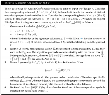
6.1.2. Elaborating Step 1
The -guess introduced in step 1 of the boxed definition conceptually implies that several cells beyond can be immediately crossed out (see item in Section 4.1.2). Conceptually again, these cell crossings are revoked when backtracks from the -guess. In reality, however, does not work with crosses, nor does the solver actually inject symbols in an actual tableau.
Recall Remark 18, where we noted that numerous formulas admit extensions. For example, formula (26) can be extended into the form of (27), shown below:
Formula (27) makes the -guess explicit—through its first conjunct. However, we opt for the dynamic generation of (26) and similar constraints, rendering the first conjunct in (27) redundant.
Claim 4.
The dynamic generation of constraint (26), along with all other Horn constraints encapsulated by , can be performed in time for some sufficiently large constant κ.
Claim 4 follows almost directly from Claim 3. To see this, first consider storing all constraints in a database using the format specified in (27) (after all). Then, when the -guess is made at runtime, prune the relevant constraints from the database and discard the first conjunct (which encodes the -guess) before passing them to .
6.1.3. Elaborating Step 3
Recall Example 8 with regard to Table 11, row index , and the coin toss outcome . Then, for each a-admissible literal * in relative to , the following two constraints must hold:
where is the a-updating cell corresponding to and *.
Now, if in step 3 the tape-state symbol is guessed for in the basic mini tableau,
then—by virtue of the left implication in (28)—the solver must incorporate the consequent as a propositional fact in its subsequent satisfiability analysis.
Conceptually, the solver injects the tape-state symbol beyond the boundaries of ; specifically, in in the basic tableau. A parallel consideration applies to in relation to the right implication in (28).
6.1.4. Complexity
Concerning the complexity of the rFHB algorithm, we begin with three observations. Observation 1 comprises three points:
-
The dimensions of the basic mini tableau are given byThe same result holds for the extended mini tableau.
-
The rFHB algorithm runs on , implying and the use of unary notation. Asymptotically, this leads to symbols per literal across the total literals in , forming the horizontal dimension of the entire tableau:For the vertical dimension, we focus on the Updating Stage, which asymptotically dominates the Coin-Tossing and Checking Stages. Here, we account for l iterations over the entire length of :Thus, the basic tableau, which is a quasi-square matrix, has the following dimensions:The same result holds for the extended tableau.
-
This indicates that as l (and thereby m) increases, the mini tableau becomes proportionally much smaller relative to the entire tableau.
Observation 2, consisting of three similar points, concerns the state of affairs had we employed a sophisticated and efficient 3-SAT solver—with and binary notation:
- The mini tableau remains unchanged: see (29).
- The horizontal dimension of the entire tableau, previously given in (30), now becomes:since only symbols per literal are needed, in contrast to l symbols. The vertical dimension, updated from (31), becomes:reflecting the fact that the Updating Stage now operates in a single (essentially right-to-left) pass. Accordingly, the tableau forms a quasi-square matrix with dimensions:
-
A devil’s advocate will attempt to minimize this expression by assuming , yielding:which, similar to the result in (33), still confirms that the mini tableau becomes proportionally smaller as l increases.
With respect to the rFHB algorithm, Observation 3 underscores that Theorem 2 from Daylight [1]—which establishes genuine compression for the case —is derived under a notably conservative assumption: the ratio between the entire tableau and the mini tableau is fixed at a constant value (specifically, 2), rather than allowed to grow with l, as is the case in results (37) and (33).
Theorem 2.
(Reproduced from Daylight [1](p. 30)) Let be a 3-SAT solver. Then the runtime of the rFHB algorithm pertaining to N satisfies the upper bound:
for some constant .
Rewriting the upper bound from Theorem 2 in terms of l, under the assumption , yields:
where the first and second cases correspond to unary and binary notation, respectively. Recall (30) and (34), respectively.
Corollary 2.
Let be a 3-SAT solver, operating in binary notation. Assume . Then, the runtime of the rFHB algorithm associated with N admits the upper bound:
for some constant .
Corollary 2 reveals genuine compression when , suggesting that machines are inferior to at least one exponential time deterministic TM. Yet rather than examining this potential novelty, we stress (again) that Corollary 2 is founded on a highly conservative premise: the hole-filling region external to the mini tableau matches the mini tableau in size for all values of l.
Remark 20.
In technical terms, we highlight that Daylight’s proof outline [1] (p. 31) treats the “reduction factor,” denoted as Δ, as a constant—rather than as a function that decreases monotonically with l, such that .
The asymptotic reality is that, as l grows, the contribution of the mini tableau becomes an increasingly negligible portion of the overall tableau. Recall (37) and (33). We now formalize this observation with the following theorem.
Theorem 3.
(Refinement of Theorem 2) Let be some machine that solves 3-SAT, with , working in unary or binary. Let l denote the number of distinct (encoded) propositional variables in the input w of . Then, the runtime of the rFHB algorithm associated with and w admits the upper bound:
where is a constant.
Remark 21.
Theorem 3 also concerns the machine , as defined in Section 4.
Proof.
We can distinguish between eight cases based on three parameters. First, we consider two values for k: either or . Second, the machine operates using either unary or binary notation. Third, we differentiate between and . In the remainder of this proof, it suffices to analyze the gravest case, which—as the reader can verify—occurs when , binary notation is used, and .
In this context, recall from (37) the following result:
which represents the smallest conceivable ratio between the size of the entire tableau and that of the mini tableau.
Furthermore, we reuse the recurrence relation from Daylight [1] (p. 31), which takes the following form:
where the constant depends on the specific TM, , under analysis. Appendix D presents a standard derivation of the solution to this recurrence relation, yielding:
Additionally, as noted by Daylight [1](p. 31), at the onset of the recurrence, p denotes the initial area of possible binary nondeterministic choices made by . Consequently, we revisit equation (36), this time replacing m with l, justified by the asymptotic relationship . Substituting for p in (39), we derive:
for some constant .
Finally, we account for the polynomial overhead per step of the rFHB algorithm, which is for some constant —recall Claims 3 and 4. Given that , it follows that our final solution is also in the form of (40). □
In light of the implication of Theorem 3, we present an alternative approach that leads to the same conclusion: an iterative application of Theorem 2 outlined in Appendix E. We now turn to the streamlined variant of the rFHB algorithm.
6.2. The sFHB Algorithm
The sFHB focuses on the operation of the coin-tossing machine , which is solely tasked with executing stage of in nondeterministic time (Section 4.1). Now we define:
where each component within the parentheses is of smaller size relative to the rFHB case. In particular, encodes only the instructions of , not . The formula characterizes the initial coin-tossing configuration (7) in Section 4.1 (without ). Similarly, the remaining three conjuncts within the parentheses pertain solely to the structure of the (extended) mini tableau, not the (extended) entire tableau.
We distinguish between two arrangements that the sFHB can make per visited column (Section 6.2.1). Then we specify the algorithm (Section 6.2.2) and elaborate on step 4 in the specification (Section 6.2.3). Finally, we present a cost analysis (Section 6.2.4).
6.2.1. Two Arrangements
As with rFHB, the sFHB algorithm performs an -guess expressed as
from which it can subsequently backtrack.
In contrast to rFHB, which processes the tableau rowwise, sFHB works across the columns (of the mini tableau). For each visited column c in the mini tableau (see, e.g., Table 11), sFHB guesses one of two possible symbol arrangements occurring at some position r among the first candidates in that column. The first possible arrangement corresponds to a coin toss yielding a 1:
while the second corresponds to a toss yielding a 0:
When sFHB selects an arrangement at column c and row r in the basic mini tableau, it introduces a separation of concerns between the columns to the left and those to the right of c. While subsequent hole-filling choices on either side will typically constrain the options on the other side, they will not affect the corresponding computations an sich. Specifically, a commitment is made—either to the first arrangement (42) or the second arrangement (43)—that constrains the tape head of to visit column c in the following manner:
The sFHB algorithm populates all remaining cells in column c—namely, those above and below , in the basic mini tableau—with designated tape symbols, in full compliance with the operation of the coin-tossing machine . Specifically, blank symbols (□) are inserted above row r in both arrangements, while the symbol 1 (respectively, 0) is written below row in the first (respectively, second) arrangement.
To illustrate the first arrangement, recall instruction (Section 4.1) and Table 11 (Section 5.1). Suppose and specifically:
where the latter conjunct implicitly refers to either or to , depending on the toss outcome for coin . Regardless of which of these two possibilities manifests, the computations to the left of column 3 in Table 11 remain unaffected. This invariance is ensured by the first conjunct in (44), which enforces the separation of concerns.
We now redefine notation (9) from Definition 7 via two examples.
Example 10.
Based on Table 11:
- (44)
- (i.e., false)
Example 11.
Based on Table 11:
6.2.2. Boxed Definition

6.2.3. Elaborating Step 4
Recall the following example of a correlated coin-tossing constraint. We have transformed the non-Horn formula (45) into the Horn formula (46).
Suppose the sFHB algorithm guesses and . Conceptually, the solver then injects the symbol 1 into of the basic tableau .
6.2.4. Complexity
Regarding the computational complexity of the sFHB algorithm, a quick, conservative estimation of the combinatorial cost associated with the separation of concerns (Section 6.2.1) is given by:
where the constant 2 refers to the two arrangements (42) and (43), and the plus sign (rather than a multiplication sign) embodies the separation of concerns.
Upon a change of variables, the recurrence relation transforms into:
which, by the standard derivation in Appendix F, yields the following approximate solution:
for some constant . The result is superpolynomial but subexponential.
This already establishes that, at a minimum, an exponential-time deterministic TM exists that outperforms every machine. Notably, this conclusion is reached independently of the cost analysis presented in [1]. Furthermore, Lemma 2 enables us to strengthen this result even further.
Lemma 2.
The runtime of the sFHB algorithm is bounded above by that of rFHB.
Proof.
It is sufficient to demonstrate that, asymptotically, the size of does not exceed that of . This claim follows directly from the cost analyses presented in Section 5.2 and Section 5.4. □
Hence, the tight upper bound for rFHB stated in inequality (38) of Theorem 3 also applies to the sFHB algorithm, which is conceptually much simpler to teach and implement.
7. Closing Remarks
A polynomially bounded tableau inherently lacks the capacity to concretely represent an exponential number of computation paths. As a result, the coin-tossing behavior of any machine must exhibit significant correlation. Crucially, as the length of the input w to machine N increases, the portion of the tableau attributable to coin tosses becomes increasingly negligible in comparison to its total size.
In this article, we have demonstrated how to quantify these properties and derive theoretical insights accordingly. To ensure a level of rigor absent from our previous work [1], we have presented our analysis in great detail. A short summary of our findings will be developed in follow-up work.
Funding
This research received no funding.
Acknowledgments
Forthcoming.
Conflicts of Interest
The author declares no conflicts of interest.
Abbreviations
The following abbreviations are used in this manuscript:
| TM | Turing Machine |
| NP | Nondeterministic Polynomial |
Appendix A.
Definition A1.
Cf. [10] (p. 259, 271). Variables that can take on the values and are called Boolean variables. We represent by 1 and by 0. The Boolean operations , , and , represented by the symbols ∧, ∨, and ¬, respectively, are described in the standard manner. We use the overbar as a shorthand for the ¬ symbol, so means . A Boolean formula is an expression involving Boolean variables and operations. It is satisfiable if some assignment of 0s and 1s to the variables makes the formula evaluate to 1. We say the assignment satisfies . The satisfiability problem is to test whether a Boolean formula is satisfiable. Let =, where refers to a standard encoding of ϕ.
Definition A2.
Cf. [10] (p. 273). A literal is a Boolean variable or a negated Boolean variable, as in x or . The former is called a positive literal, while the latter is called a negative literal. A clause is several literals connected with ∨s, as in . A Boolean formula is in conjunctive normal form, called a cnf formula, if it comprises clauses with ∧s, as in ∧∧ . The Boolean formula is a 3cnf formula if each clause has three literals, as in ∧∧ . A 2cnf formula is an of clauses, where each clause is an of at most two literals.
Definition A3.
Cf. [20] (p. 34–35). A (propositional) Horn formula is a cnf formula where every disjunction contains at most one positive literal.
Also, =.
Remark A1.
Horn clauses can be written as implications by the following equivalence (≡):
Theorem A1.
Cf. [20] (p. 35). .
Definition A4.
Cf. Sipser [10] (p. 140). A deterministic Turing machine is an 8-tuple
, with T finite sets:
| Q is the set of states, and is the input alphabet not containing the blank symbol □. |
| is the tape alphabet, where and . |
| is the transition function. |
| Every transition in is accompanied by a distinct label t. |
| T is the label set, containing all such labels. |
| is the start state. |
| is the accept state. is the reject state, with . |
As a Turing machine computes, changes occur in the current state, the current tape contents, and the current head location. A setting of these three items is called a configuration of the Turing machine. The tape of the Turing machine is one-way infinite, from left to right. Specifically, for each input of length n, machine M starts in configuration , for , and in configuration , for . In both cases, the notation , with , signifies that the head is located at the tape cell containing symbol s, while the machine resides in state . Machine M neither starts in or , nor progresses beyond either one of these states. Specifically, once M reaches , it remains active solely in that state. Likewise for . We take to be some with and similarly for . Input word w is considered accepted when M on w reaches . We write to denote the language accepted by M. We use notation when referring to some transition in δ with label and movement . The plus sign (minus sign) signifies a movement to the right (to the left).
Definition A5.
Cf. Sipser [10] (p. 150). A nondeterministic Turing machine is an 8-tuple, , . At any point in a computation, the machine may proceed according to several possibilities. The transition function for the machine has the form , where denotes the power set. The computation of the machine is a tree whose branches correspond to different possibilities for the machine. If some branch of the computation leads to the state , the machine accepts its input.
In conformity with Definition A4, each transition in set δ is accompanied by a distinct label t, and T is now called the general label set, containing all such labels. For instance, consider notation , with label , states , symbols , movements , and with tuple different from . This notation captures the nondeterministic transition encompassing the deterministic transitions and . We define the basic label set, denoted as , as the set that encompasses the labels of all deterministic transitions, such as and .
Remark A2.
In our discussion, we employ the term “nondeterministic transition” explicitly, while abbreviating “deterministic transition” and “basic label set” to simply “transition” and “label set.” We frequently omit brackets for ease of reading; e.g., we write t and instead of and . The crux is that each basic label is unique.
Definition A6.
Consider an arbitrary nondeterministic Turing machine, N, and its basic label set, . For any label t in with corresponding signature or , we let “” “” and “” stand for the symbols and , respectively. When machine N is clear from the context, we shall simply note down “” “” and “,” respectively.
Definition A7.
Consider an arbitrary nondeterministic Turing machine, N, and its general label set, T. We let denote the subset of T containing the labels of all deterministic instructions of N. We let , respectively , denote the subset of containg the labels of all deterministic instructions of N whose movement is to the right (+), respectively to the left (−).
Definition A8.
Let N be a nondeterministic Turing machine decider. Its running time is function , with the maximum number of steps N uses on any branch of its computation, on any input of length n, before halting.
Definition A9.
Cf. [10](pp. 251, 258). Let be a function, with denoting the set of nonnegative real numbers. Define the time complexity class, , to be the collection of all languages that are decidable by an time Turing machine. is the class of languages that is decidable in polynomial time on a deterministic single-tape Turing machine. In other words, .
Theorem A2.
Cf. [20](p. 35). .
Definition A10.
Cf. [10](pp .265–267). A verifier for a language A is an algorithm V, where A =
. We measure the time of a verifier only in terms of the length of w, so a polynomial time verifier runs in polynomial time in the length of w. A language A is polynomial verifiable if it has a polynomial time verifier. is the class of languages that have polynomial time verifiers.
The remaining three items come from [10, p.266-276].
Theorem A3.
A language is in iff it is decided by some nondeterministic polynomial time Turing machine.
Definition A11.
=. A function is a polynomial time computable function if some deterministic polynomial time Turing machine M exists that halts with just on its tape, when started on any input w. A language B is -complete if it satisfies two conditions: (1) B is in , and (2) every A in is polynomial time reducible to B.
Theorem A4.
If B is -complete and , then .
Appendix B.
Appendix B.1. The Single Part
We define as follows:
where , , and the column index ranges from 1 to . This condition ensures that if the tape-state symbol is stored in , it is the only tape-state symbol in row . In other words, no tape-state symbol can be stored in any other cell within the same row.
Appendix B.2. The Left Part
We define as follows:
On the one hand, we reason from row i both towards earlier rows () and towards later rows ():
where the restriction on , denoted by , is defined by the following inequalities:
Additionally, the expression
is shorthand for:
where is defined as the maximum (not the minimum) of the set:
Similarly, is defined as the maximum of the set:
Example A1.
For instance, if and hold, with , then the following must also hold:
where is defined by the following inequalities:
The reader can verify that all relevant cells range from at the top to at the bottom. These cells correspond to the 13 crossed-out entries in column in Table 7.
On the other hand, we reason from the earliest row () and, respectively, the latest row () toward row i, with :
The satisfiability of ensures that if a specific cell, such as
for some fixed m, is filled with the tape symbol , then—through a chain reaction partially facilitated by —all crosses in column are replaced with the symbol . A similar observation applies to the satisfiability of , which affects the propagation from an earlier cell, i.e.,
Appendix B.3. The Right Part
Given the inherent symmetry of the problem, the formal definition of closely mirrors that of and is therefore omitted from this paper.
Appendix B.4. The Extend Part
Here, represent two distinct labels of the machine N, such that:
Recall Definition A6. The minus (plus) sign indicates that N moves to the left (right).
Appendix B.5. Consolidation
In summary, is a Horn formula, with a size of , where the constant k corresponds to the running time of machine N.
Appendix C.
We can readily formulate several more constraints. For instance, let us continue with and Table 11. Suppose that, in the mini tableau, the coin toss outcome has materialized:
Now, consider the cell —positioned at row and column , beyond the confines of the first rows of the mini tableau—for which the following proposition holds:
In other words, relative to the cell , one time step earlier and one cell to the right, the head is scanning a bit b while in state . This state of affairs is exemplified by the following configuration and :
In conformity with instructions and —recall from Section 4.2.4:
—we then posit that
must hold. Here, the tape-state symbol signifies that the TM’s head is scanning—from right to left—in search of the first occurrence of a symbol located to the left of the bit 1 in cell . (When such a is found, the machine overwrites it: replacing a with 0 and with 1.)
Formally, these long-range dependencies are captured by the following constraints—each a Horn formula with three literals:
Conservatively, this yields a complexity of:
Appendix D.
To solve the recurrence relation, we begin with the following setup:
where is a constant.
Step 1: Change of Variables
Let us set:
Now consider the recurrence:
Let:
Then the recurrence becomes:
Taking logarithms (base 2) on both sides:
Let:
so the recurrence becomes:
Step 2: Solve the Linear Recurrence
Unrolling the recurrence for n steps:
To reach the base case , choose:
Then:
Recalling that , we obtain:
Exponentiating both sides:
where:
Thus, the solution is:
Asymptotic Behavior as l→∞
As , we have:
so:
Then:
and thus:
for some constant .
Hence, asymptotically:
as . This implies that is polynomial in p, and the degree becomes smaller as l increases.
Appendix E.
We apply Theorem 2 iteratively to establish the validity of Theorem 3.
Appendix E.1. First Iteration
Theorem 2 conveys that any 3-SAT solver , with state set and tape alphabet —operating with nondeterministic binary guesses followed by deterministic verification time—can be simulated deterministically by some via the rFHB algorithm.
Via a single application of Theorem 2, the resulting deterministic TM runs in at most
time, where:
- The constant depends on the sizes of and .
- The constant .
Inspired by the existence of deterministic machine , we can now construct a nondeterministic polynomial time TM , with state set and tape alphabet where
This machine is functionally equivalent to , and hence is also a 3-SAT solver.
At first glance, operates with
nondeterministic binary guesses, followed by
deterministic verification time. Recall Claim 3.
Upon closer inspection, operates with, say,
nondeterministic binary guesses. An arbitrary small but nonzero increase in the number of guesses (from to ) is required here, for the following reason: guesses (and correctly so, in the satisfiable case) the guesses made by rFHB relative to . Although the total number of holes is , rather than linear in n, an additional bits are needed to uniquely identify each guess within the tableau. Consequently, makes
binary guesses, which we simplify to for subsequent analysis.
To recatipulate, functionally equivalent machines and require and guesses, respectively. For sufficiently large n, machine makes fewer guesses than .
Appendix E.2. Second Iteration
Via a second application of Theorem 2, we may infer the existence of a deterministic machine that simulates the nondeterministic machine . This machine runs in at most
time, where:
- The constant .
- depends on the sizes of and , with .
Inspired by the existence of deterministic machine , we can now construct a functionally equivalent nondeterministic polynomial time TM , with state set and alphabet , where
This machine operates, not with
but with, say,
nondeterministic binary guesses, followed by
verification time. Again, the rationale for the slight increase in the exponent is due to the extra bits that are needed to uniquely identify each guess within the tableau.
To recatipulate, and require and guesses, respectively. For sufficiently large n, machine makes fewer guesses than .
Appendix E.3. Third Iteration
Via a third application of Theorem 2, we may infer the existence of a deterministic TM that simulates the nondeterministic machine . And so on.
Appendix E.4. The j-th Iteration
Inspired by the existence of deterministic machine , we can now construct a functionally equivalent, nondeterministic polynomial time TM , with state set and tape alphabet , where
This machine operates, not with
but with, say,
nondeterministic binary guesses, followed by
verification time.
Appendix E.5. Consolidation
Take , for some sufficiently large constant . Then machine performs guesses, followed by
deterministic verification time. That is, is a deterministic polynomial time TM.
Appendix F.
Solve the recurrence relation:
where is a constant.
Solution
Assume . Then the recurrence becomes:
Apply the recurrence repeatedly:
Now simplify the exponent:
Therefore:
Substituting back , we get:
Asymptotic Form
As ,
which implies that the growth rate is quasi-polynomial—faster than any polynomial, yet slower than exponential.
References
- Daylight, E.G. Tableau with Holes: Clarifying NP-Completeness. Symmetry 2025, 17. [CrossRef]
- Daylight, E. Injecting Observers into Computational Complexity. Philosophies 2025, 10. [CrossRef]
- Dean, W. Computational Complexity Theory. The Stanford Encyclopedia of Philosophy 2016.
- Fortnow, L. Why Can’t We Break Cryptography? https://blog.computationalcomplexity.org/2025/04/why-cant-we-break-crytptography.html, 2025. Accessed: 2025-07-01.
- Li, M.; Vitanyi, P. An Introduction to Kolmogorov Complexity and Its Applications, 4 ed.; Texts in Computer Science, Springer, 2019. [CrossRef]
- Daylight, E.; Koolen, W.; Vitányi, P. Time-Bounded Incompressibility of Compressible Strings and Sequences. Information Processing Letters 2009, 109, 1055–1059. [CrossRef]
- Cook, S. The Complexity of Theorem-Proving Procedures. In Proceedings of the Proc. 3rd Annual ACM Symposium on Theory of Computing. Association for Computing Machinery, 1971, pp. 151–158.
- Levin, L. Universal Sorting Problems. Problems of Information Transmission 1973, 9, 265–266. English translation of original in Problemy Peredachi Informatsii.
- Fortnow, L.; Homer, S. A Short History of Computational Complexity. Bulletin of the European Association for Theoretical Computer Science 2003, 80, 95–133.
- Sipser, M. Introduction to the Theory of Computation; Thomson Course Technology, 2006.
- Papadimitriou, C. Computational Complexity; Addison Wesley Longman, 1994.
- Hopcroft, J.; Motwani, R.; Ullman, J. Introduction to Automata Theory, Languages, and Computation; Addison Wesley / Pearson Education, 2007.
- Aaronson, S. Quantum Computing since Democritus; Cambridge University Press, 2013.
- Dean, W. Algorithms and the Mathematical Foundations of Computer Science. In Gödel’s Disjunction, First ed.; Horsten, L.; Welch, P., Eds.; Oxford University Press, 2016.
- Tall, D. How Humans Learn to Think Mathematically: Exploring the Three Worlds of Mathematics; Cambridge University Press, 2013.
- Turner, R. Computational Abstraction. Entropy 2021, 23, 213. [CrossRef] [PubMed]
- Linnebo, .; Shapiro, S. Actual and Potential Infinity. Noûs 2019, 53, 160–191. [CrossRef]
- Fortnow, L. Can you feel the machine? https://blog.computationalcomplexity.org/2024/03/can-you-feel-machine.html, 2024. Accessed: 2024-08-22.
- Hill, R.K. The Imperativity of Algorithms. https://cacm.acm.org/blogcacm/the-imperativity-of-algorithms/, 2023. Accessed: 2024-08-22.
- Grädel, E. Complexity Theory: WS 2009/10; Mathematische Grundlagen der Informatik, RWTH Aachen, creativecommons.org, 2009.
- Dowling, W.; Gallier, J. Linear-Time Algorithms for Testing the Satisfiability of Propositional Horn Formulae. J. Logic Programming 1984, 1, 267–284. [CrossRef]
- Daylight, E. Dijkstra’s Rallying Cry for Generalization: the Advent of the Recursive Procedure, late 1950s – early 1960s. The Computer Journal 2011, 54, 1756–1772. [CrossRef]
- Shapiro, S. Acceptable notation. Notre Dame Journal of Formal Logic 1982, 23, 14–20. [CrossRef]

Table 1.
A tableau: an matrix. All cells in the leftmost column contain the boundary marker ⊢. Likewise for the rightmost column and the marker ⊣.
Table 1.
A tableau: an matrix. All cells in the leftmost column contain the boundary marker ⊢. Likewise for the rightmost column and the marker ⊣.
| ⊢ | … | □ | … | □ | ⊣ | ||||
| ⊢ | ⊣ | ||||||||
| ⊢ | ⊣ | ||||||||
| |
|||||||||
| ⊢ | ⊣ |
Table 2.
Illustrating two windows. The effect of instruction is shown on the left, while the effect of instruction is displayed on the right, with both illustrations read from top to bottom. Column indices range from to . Each vertical arrow represents a change in precisely one symbol. Notably, is considered a single symbol, not two separate symbols.
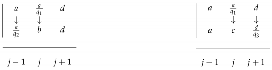 |
Table 3.
The effect of instruction is shown on the left, while the effect of is displayed on the right. In both illustrations, the rows are arranged sequentially from the top row, indexed as , to the bottom row, indexed as . Each vertical arrow represents a change in precisely one symbol. If label is stored in of the tableau—with row index and column index j, where l and j are natural numbers—then we denote this with propositional variable . Source: [2](p. 15).
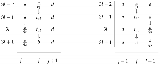 |
Table 4.
A conversion from symbol a (marked in the top row) to b (marked in the bottom row). Row indices range from to . Column indices from 2 to 5. Source: [2](p. 6, original emphasis]).
Table 4.
A conversion from symbol a (marked in the top row) to b (marked in the bottom row). Row indices range from to . Column indices from 2 to 5. Source: [2](p. 6, original emphasis]).
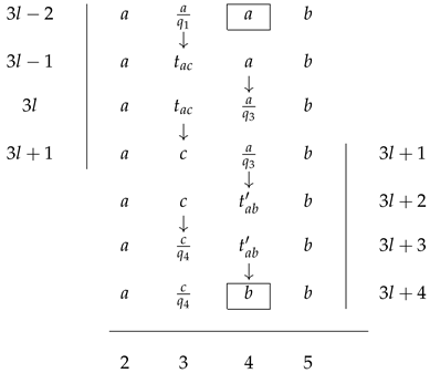 |
Table 5.
Here, the proposition holds, with . In words: in the extended tableau contains the tape-state symbol .
Table 5.
Here, the proposition holds, with . In words: in the extended tableau contains the tape-state symbol .
| × | × | × | × | × | |||||||
| × | × | × | × | × | × | ||||||
| × | × | × | × | × | × | × | × | ||||
| i | × | × | × | × | × | × | × | × | × | × | |
| × | × | × | × | × | × | × | × | ||||
| × | × | × | × | × | × | ||||||
| × | × | × | × | × | |||||||
| × | × | × | × | ||||||||
| × | × | × | |||||||||
| × | × | ||||||||||
| × | |||||||||||
| j |
Table 6.
Here, the proposition holds. This means that the symbol appears at position in the basic tableau (shown below), with .
Table 6.
Here, the proposition holds. This means that the symbol appears at position in the basic tableau (shown below), with .
| × | × | × | × | × | |||||||
| × | × | × | × | × | × | ||||||
| × | × | × | × | × | × | × | × | ||||
| × | × | × | × | × | × | × | × | × | × | ||
| × | × | × | × | × | × | × | × | ||||
| × | × | × | × | × | × | ||||||
| × | × | × | × | × | |||||||
| × | × | × | × | ||||||||
| × | × | × | |||||||||
| × | × | ||||||||||
| × | |||||||||||
| j |
Table 7.
Filling cells (in the extended tableau) with additional crosses as a logical consequence of the state of affairs depicted in Table 5 and
Table 7.
Filling cells (in the extended tableau) with additional crosses as a logical consequence of the state of affairs depicted in Table 5 and
| × | × | × | × | × | |||||||
| × | × | × | × | × | |||||||
| × | × | × | × | × | |||||||
| × | × | × | × | × | × | ||||||
| × | × | × | × | × | × | ||||||
| × | × | × | × | × | × | ||||||
| × | × | × | × | × | × | × | × | ||||
| × | × | × | × | × | × | × | × | ||||
| × | × | × | × | × | × | × | × | ||||
| i | × | × | × | × | × | × | × | × | × | × | |
| × | × | × | × | × | × | × | × | ||||
| × | × | × | × | × | × | × | × | ||||
| × | × | × | × | × | × | × | × | ||||
| × | × | × | × | × | × | ||||||
| × | × | × | × | × | × | ||||||
| × | × | × | × | × | × | ||||||
| × | × | × | × | × | |||||||
| × | × | × | × | × | |||||||
| × | × | × | × | × | |||||||
| × | × | × | × | ||||||||
| × | × | × | × | ||||||||
| × | × | × | × | ||||||||
| × | × | × | |||||||||
| × | × | × | |||||||||
| × | × | × | |||||||||
| × | × | ||||||||||
| × | × | ||||||||||
| × | × | ||||||||||
| × | |||||||||||
| × | |||||||||||
| × | |||||||||||
| j |
Table 8.
Basic tableau: crossing out 113 cells out of cells.
| 1 | × | |||||||||||||||
| × | × | × | ||||||||||||||
| × | × | × | × | × | ||||||||||||
| × | × | × | × | × | × | × | ||||||||||
| 5 | × | × | × | × | × | × | × | × | × | |||||||
| × | × | × | × | × | × | × | × | × | × | × | ||||||
| × | × | × | × | × | × | × | × | × | × | × | × | × | ||||
| 8 | × | × | × | × | × | × | × | × | × | × | × | × | × | × | × | |
| × | × | × | × | × | × | × | × | × | × | × | × | × | ||||
| 10 | × | × | × | × | × | × | × | × | × | × | × | |||||
| × | × | × | × | × | × | × | × | × | ||||||||
| × | × | × | × | × | × | × | ||||||||||
| × | × | × | × | × | ||||||||||||
| × | × | × | ||||||||||||||
| 15 | × | |||||||||||||||
| 16 | ||||||||||||||||
| 1 | 2 | 3 | 4 | 5 | 6 | 7 | 8 | 9 | 10 | 11 | 12 | 13 | 14 | 15 | 16 |
Table 9.
Basic tableau: a second intervention in row 4 amounts to crossing out 41 boldfaced cells out of 63 cells in rows 1–7. The depicted scenario is ultimately unsatisfiable, as the downward movement from and the upward movement from will fail to converge harmoniously in the same cell.
Table 9.
Basic tableau: a second intervention in row 4 amounts to crossing out 41 boldfaced cells out of 63 cells in rows 1–7. The depicted scenario is ultimately unsatisfiable, as the downward movement from and the upward movement from will fail to converge harmoniously in the same cell.
| 1 | × | × | × | × | × | × | × | × | × | |||||||
| × | × | × | × | × | × | × | × | × | × | × | ||||||
| × | × | × | × | × | × | × | × | × | × | × | × | × | ||||
| × | × | × | × | × | × | × | × | × | × | × | × | × | × | × | ||
| 5 | × | × | × | × | × | × | × | × | × | × | × | × | × | × | ||
| × | × | × | × | × | × | × | × | × | × | × | × | × | × | |||
| × | × | × | × | × | × | × | × | × | × | × | × | × | × | |||
| 8 | × | × | × | × | × | × | × | × | × | × | × | × | × | × | × | |
| × | × | × | × | × | × | × | × | × | × | × | × | × | ||||
| 10 | × | × | × | × | × | × | × | × | × | × | × | |||||
| × | × | × | × | × | × | × | × | × | ||||||||
| × | × | × | × | × | × | × | ||||||||||
| × | × | × | × | × | ||||||||||||
| × | × | × | ||||||||||||||
| 15 | × | |||||||||||||||
| 16 | ||||||||||||||||
| 1 | 2 | 3 | 4 | 5 | 6 | 7 | 8 | 9 | 10 | 11 | 12 | 13 | 14 | 15 | 16 |
Table 10.
The coin-tossing section of the basic tableau, also known as the basic mini tableau [1]: tossing four coins from left to right, resulting in the truth values for variables and The row corresponds to the state attained after all coins have been tossed and when the rightmost column is reached. In this case, l is even. Consequently, is odd and belongs to the set .
| 1 | # | − | # | |||
| 2 | − | − | ||||
| 3 | − | − | ||||
| 4 | − | − | ||||
| 5 | − | · | − | |||
| 6 | − | · | ||||
| 7 | − | · | ||||
| 8 | − | · | ||||
| 9 | − | · | ||||
| 10 | − | |||||
| 11 | − | · | ||||
| 12 | − | |||||
| 13 | − | |||||
| 1 | 2 | 3 | 4 | 5 | 6 |
Table 11.
The basic mini tableau: tossing coins from left to right, resulting in the truth values for and The row corresponds to the state attained after all coins have been tossed and when the rightmost column is reached. In this case, l is odd. Consequently, is even and belongs to the set .
Table 11.
The basic mini tableau: tossing coins from left to right, resulting in the truth values for and The row corresponds to the state attained after all coins have been tossed and when the rightmost column is reached. In this case, l is odd. Consequently, is even and belongs to the set .
| 1 | # | − | # | ||
| 2 | − | − | |||
| 3 | − | − | |||
| 4 | − | − | |||
| 5 | − | · | |||
| 6 | − | · | |||
| 7 | − | ||||
| − | · | ||||
| 9 | − | ||||
| 10 | − | ||||
| 1 | 2 | 3 | 4 | 5 | |
Table 12.
Illustrating on the left and on the right.
| 1 | # | − | # | 1 | # | − | # | |||||
| 2 | − | − | 2 | − | − | |||||||
| 3 | − | 3 | − | − | ||||||||
| 4 | − | − | 4 | − | − | |||||||
| 5 | − | 5 | − | |||||||||
| 6 | − | · | 6 | − | · | |||||||
| 7 | − | 7 | ||||||||||
| 8 | − | · | 8 | − | · | |||||||
| 9 | − | 9 | ||||||||||
| 10 | − | 10 | − | |||||||||
| 11 | # | # | 11 | # | # | |||||||
| 1 | 2 | 3 | 4 | 5 | 1 | 2 | 3 | 4 | 5 |
Table 13.
Two distinct computations in the making: one on the left and the other on the right.
| 1 | # | − | # | 1 | # | − | # | |||||
| 2 | − | − | 2 | − | − | |||||||
| 3 | − | 3 | − | − | ||||||||
| 4 | − | − | 4 | − | − | |||||||
| 5 | 5 | |||||||||||
| 6 | − | · | 6 | − | · | |||||||
| 7 | − | 7 | ||||||||||
| 8 | − | · | 8 | − | · | |||||||
| 9 | − | 9 | − | |||||||||
| 10 | − | 10 | − | |||||||||
| 11 | # | # | 11 | # | # | |||||||
| 1 | 2 | 3 | 4 | 5 | 1 | 2 | 3 | 4 | 5 |
Table 14.
Two distinct computations taking shape, with only the left one remaining potentially satisfiable.
Table 14.
Two distinct computations taking shape, with only the left one remaining potentially satisfiable.
| 1 | # | − | # | 1 | # | − | # | |||||
| 2 | − | 1 | − | 2 | − | − | ||||||
| 3 | 1 | 3 | − | − | ||||||||
| 4 | − | − | 4 | − | − | |||||||
| 5 | 1 | 5 | 1 | |||||||||
| 6 | 1 | − | · | 6 | 1 | − | · | |||||
| 7 | − | 7 | 1 | |||||||||
| 8 | − | · | 8 | 1 | − | · | ||||||
| 9 | − | 9 | − | |||||||||
| 10 | − | 10 | − | |||||||||
| 11 | # | # | 11 | # | # | |||||||
| 1 | 2 | 3 | 4 | 5 | 1 | 2 | 3 | 4 | 5 |
Disclaimer/Publisher’s Note: The statements, opinions and data contained in all publications are solely those of the individual author(s) and contributor(s) and not of MDPI and/or the editor(s). MDPI and/or the editor(s) disclaim responsibility for any injury to people or property resulting from any ideas, methods, instructions or products referred to in the content. |
© 2025 by the authors. Licensee MDPI, Basel, Switzerland. This article is an open access article distributed under the terms and conditions of the Creative Commons Attribution (CC BY) license (http://creativecommons.org/licenses/by/4.0/).
Copyright: This open access article is published under a Creative Commons CC BY 4.0 license, which permit the free download, distribution, and reuse, provided that the author and preprint are cited in any reuse.


