Submitted:
28 July 2025
Posted:
29 July 2025
You are already at the latest version
Abstract
Planetary exploration missions have acquired a growing amount of remote sensing data, offering a reliable basis for studying the geological evolution of planetary bodies, such as Mars. In recent years, machine learning models have emerged as powerful tools for remote sensing by providing scalable and adaptive solutions for planetary science. In this study, we present an unsupervised machine learning framework for identifying and mapping the spatial distribution of minerals on Mars. Our framework utilises the Self-Organising Map (SOM) model and k-means clustering to identify clusters of spectral signatures, which may correspond to distinct minerals. Although the clusters can be labelled by referencing a spectral library, our framework does not require labelled data and can operate in an unsupervised manner. The framework retains full spectral dimensionality of input features while enabling topology-preserving clusters. The results indicate that our framework can identify the spatial distribution of minerals on Mars, even in complex spectral environments with overlapping features. Furthermore, the topological structure of mineral groupings that the SOM model preserves can provide important insights, including the indication of isolated minerals that may otherwise remain undetected in the target region.
Keywords:
Mars mineralogy
; hyperspectral imaging
; deep learning
; self-organised maps
; unsupervised clustering and remote sensing
1. Introduction
Since the start of its mission in 2006, the Compact Reconnaissance Imaging Spectrometer for Mars (CRISM) [1] has delivered high-resolution hyperspectral observations of the Martian surface. Hyperspectral sensors capture data across hundreds of spectral bands, which have enabled more precise material and terrain identification compared to traditional remote sensing techniques [2]. This advancement, combined with an increasing number of hyperspectral datasets, has led to increasing research interest in hyperspectral remote sensing data over time [3,4]. The CRISM Targeted Empirical Record (TER) [5] product suite, released in 2016, offers atmospherically and photometrically corrected hyperspectral data for targeted regions of Mars. This data offers valuable information on the composition and spatial distribution of surface minerals, thereby contributing to our understanding of the planet’s geological history and past environmental conditions [6,7,8].
Overtime, hyperspectral data has become the primary tool for large-scale mineral mapping on Mars [7,9]. Similar hyperspectral frameworks have proven valuable in both planetary and terrestrial contexts. For example, the The Moon Mineralogy Mapper is a state of-the-art imaging spectrometer designed to provide high spectral resolution data across large areas of the Moon’s surface, with the goal of identifying mineral and rock compositions [10]. A comprehensive understanding of the lunar surface is essential in preparation for future crewed Artemis missions [11] that aim to establish a long-term presence on the Moon [12]. On Earth, terrestrial mineral exploration has exploited hyperspectral data from airborne and satellite sensors, demonstrating the value of such workflows for geological mapping [13]. Furthermore, Thomas et al. [14] highlighted the application of hyperspectral infrared analysis in the study of hydrothermal alteration, underscoring the broad applicability of spectral interpretation methods across planetary surfaces.
Extracting meaningful spectral-spatial information from hyperspectral data has traditionally relied on expert judgment and manual processes [3,15], which may not be suitable for large scale mineral mapping due to the risk of error or omission [7]. We encountered inconsistencies in the selection of appropriate parameters [16], resulting in inconsistent formulas and outputs. Although we employed manually adjusted pre-defined parameters to demonstrate the effectiveness of a SOM model, it is recommended that feature extraction be automated in future work, as such inconsistencies highlight the limitations of manual parameter selection. Challenges such as these are a key reason machine learning and deep learning methods have emerged as valuable tools in remote sensing [2,17] owing to their ability to capture complex, nonlinear relationships in high-dimensional remote sensing data [17]. Deep learning methods in particular, have enabled automated feature extraction and improved classification performance [3,4]. For example, Shirmard et al. [18] utilised Convolutional Neural Networks (CNNs) and multispectral remote-sensing data to classify lithological units, with almost all test samples predicted correctly - a task that can require a large number of participants and resources if performed manually.
Mars presents unique challenges for hyperspectral remote sensing, surpassing those typically experienced with terrestrial or lunar datasets. In addition to issues such as size, high dimensionality, noise, atmospheric effects [19] and spatial variability of spectral signatures [13], further complications include coarse spatial resolution, spectral ambiguity due to overlapping or subdued absorption features and atmospheric residual absorptions [9,14,15], as well as surface contaminants such as dust cover and complex surface mixtures [8,9,20,21]. These challenges are compounded by the limited availability of validation data. As a result, Mars serves as an ideal test-bed for evaluating advanced data-driven methods in sparse and noise-prone environments.
The lack of validation data poses a problem for many machine learning applications. Therefore, strategies such as transfer learning are increasingly being explored for geospatial applications. However, these strategies do not always generalise well to the target domain [22] and still benefit from some labelled data from the target domain for fine-tuning purposes [23]. In this context, unsupervised learning, particularly clustering-based approaches have become alternatives for hyperspectral data analysis [15]. Self-Organising Maps (SOMs) [24] are unsupervised neural networks used for clustering high-dimensional data onto a two-dimensional grid while preserving topological relationships [24,25,26].
SOMs have been applied across a variety of remote sensing and Earth science contexts. SOMs have been used to cluster hyperspectral data from Baffin Island, achieving reliable differentiation of spectral features and outperforming other techniques in the presence of substantial noise [27]. In geoscientific studies, SOMs have shown promise in clustering geochemical data to identify prospective gold deposits in northern Finland [28]. More recently, SOMs have been employed to identify potential landing sites near the lunar South Pole by integrating multi-source remote sensing data, revealing spatial patterns constrained by scientific and engineering considerations [29]. These examples highlight the versatility of SOMs as a tool for unsupervised pattern recognition and feature extraction in remote sensing, geological, and planetary science research.
In this study, we present an unsupervised machine learning framework to identify and map the spatial distribution of minerals on Mars. Our framework employs SOM and k-means clustering methods to identify clusters of spectral signatures, which may correspond to different minerals. Although the clusters are labelled by referencing a spectral library, the method does not require labelled data and can operate in an unsupervised manner. The framework retains full spectral dimensionality of input features while enabling topology-preserving clusters. Our framework aims to identify minerals on the Martian surface along with their spatial distribution, even in complex spectral environments with overlapping features. This provides an interpretable and adaptable approach for exploring mineral distributions in the absence of ground truth data. More broadly, the objective is to advance the automation, interpretability, and scalability of mineral mapping for planetary exploration.
Our framework explores selected regions of Mars where diagnostically interpretable remote sensing data for mineral classification exists. We derived data from the MRO CRISM Type Spectra Library, which contains a limited set of spectra for known Martian minerals. This enables a post-processing spectral matching step, where each cluster’s representative feature weights are compared to processed reference spectra from the library. The clusters formed by the SOM can be partially labelled based on the correlation between SOM-derived features and the processed spectral signatures of known Martian minerals contained within the library.
2. Background and Related Work
2.1. CRISM
Aboard NASA’s Mars Reconnaissance Orbiter (MRO), CRISM [30] is a high resolution visible-to-near-infrared (VNIR) imaging spectrometer provideing up to 544 spectral bands across the 0.362 to 3.92 range, operating in targeted and mapping modes. The mission has produced numerous data records such as EDR (Experiment Data Record) [31], TRDR (Targeted Reduced Data Record) [31], TER (Targeted Empirical Records) [31], and MTRDR (Map Projected Targeted Reduced Data Record) [31], each reflecting different levels of calibration and spatial processing [31]. These datasets have played an important role in the exploration of Martian minerals by enabling the identification of minerals associated with past aqueous activity [31].
2.2. Summary Products for Data Processing
A key challenge is the variability in raw hyperspectral data, which can arise from factors such as atmospheric effects, illumination differences, surface scattering [32] and other environmental or acquisition-related influences. Spectral parameters can be used to overcome some of these difficulties, as it may not be necessary to assess the entire spectrum to identify a mineral, but rather specific spectral features which can be described by a single parameter value [33]. Spectral parameters are widely used in CRISM data products and have proven to be a successful method of collapsing spectral variation into a limited number of dimensions to identify the presence of a mineral on Mars [34], we refer to the spectral parameters as summary products to remain consistent with Viviano et al. [34]. These summary products offer several advantages over raw hyperspectral bands by (1) emphasising mineralogically meaningful absorption features, (2) reducing dimensionality while preserving domain-relevant information, and (3) improving comparability across regions with differing photometric conditions [35]. Although summary products offer these advantages over raw hyperspectral bands, developing them is inherently time-consuming, requires expert geological knowledge, and is subject to differing expert opinions on optimal formulations [15].
We compute BD1750_2 using hyperspectral data from the MRO CRISM Type Spectra Library as an illustrative example to demonstrate the intent of a summary product. This summary product estimates absorption near m via:
The parameters a and b are weighting factors with . The value of b is approximately , the exact ratio depends on the specific wavelengths selected, which is influenced by the kernel width. Figure 1a,b illustrate the absorption feature.
As shown in Figure 1c, the summary product is sensitive primarily to Gypsum and Alunite among the 31 MRO CRISM Type Spectra Library minerals, consistent with earlier studies [34]. Notably, the absorption features remain clear even when applied to unnormalised TER-3 data, demonstrating robustness - though normalisation is recommended if a reliable reference pixel can be identified.
This study uses 29 summary products as features for mineral classification. Although the summary products are precomputed in MTRDR files, we identified discrepancies between MTRDR outputs and the official CRISM DPSIS definitions and recalculated all 29 products from TER-3 data, which was necessary to ensure the SOM input features accurately reflect the intended spectral diagnostics. Refer to Appendix B for the 29 summary products and corrections.
All 29 features were retained without applying additional dimensionality reduction techniques, such as PCA or feature selection. This was done to preserve the full range of spectral information encoded in the summary products, ensuring the SOM remained sensitive to subtle but potentially important variations in mineral signatures across the target regions.
2.3. Unsupervised Machine Learning
Dimensionality reduction methods such as Principal Component Analysis (PCA) [27,36], Minimum Noise Fraction (MNF) [19] have been used to process hyperspectral data. PCA extracts orthogonal components based on variance, which can inadvertently prioritise noise over subtle but important absorption features. MNF aims to separate signal from noise more explicitly, but may still obscure localised mineralogical signatures.
Traditional clustering algorithms such as PCA, K-means [17,36], Gaussian Mixture Models (GMM) [15,36], and DBSCAN (Density-based clustering) have been applied to hyperspectral datasets [36,37]. However, these methods come with limitations, including the need for hyperparameter tuning and assumptions about the underlying distribution of materials. Spectral unmixing approaches such as Linear Mixing Models (LMM) [38] offer an alternative by modelling each pixel as a linear mixture of spectra from a predefined set of endmembers. However, their effectiveness is limited by the linear assumption [39] and the reliance of a fixed spectra library, which may not capture the substantial spectral variability experienced in practice [39,40,41]. A SOM model can mitigate some of these limitations via the preservation of topological relationships. For instance, an over-dimensionalised SOM will produce an organised map of similar neurons that can be grouped or visually identified, meaning hyperparameter tuning is not as problematic. Similarly, topology separates high confident regions with more distinct mineral signatures from areas with more complex and mixed surface compositions, allowing for the identification of regions where spectral variability is not as problematic.
Figure 1.
Visualisation of the BD1750_2 spectral product and its diagnostic role in mineral detection. 1(a) and 1(b) show how the m absorption feature is identified using anchor bands. 1(c) highlights Gypsum and Alunite as the only minerals from the MRO CRISM Type Spectra Library with significant BD1750_2 responses.
Figure 2.
This heatmap illustrates how summary products serve as input features. Rather than displaying all 29 products for each pixel, it shows a subset of recalculated summary products for selected minerals from the MRO CRISM Type Spectra Library, highlighting spectral variation across mineral types. Each horizontal row can be thought of as an individual pixel from a TER-3 image file.
2.3.1. SOM
A SOM model projects high-dimensional inputs onto a two-dimensional topological grid while preserving neighbourhood relationships [24,25,26,42]. They are valued for their interpretability and have been successfully applied in remote sensing tasks such as cloud type classification [42], land cover classification [43], identifying distinct types of regolith and bedrock [44] and even reconstructing underwater sound speed profiles [45]. Some key advantages of a SOM model in this context include:
- High-dimensional Input Handling: A SOM model can process high-dimensional data directly without requiring dimensionality reduction (aside from computational performance considerations). Although SOMs typically use Euclidean distance (which assumes the linearity of the input space), other distance metrics can be adopted.
- Topological Preservation: Unlike traditional clustering algorithms, a SOM model preserves the topological structure of the input space. This is particularly useful in hyperspectral analysis and can reveal distinct and isolated mineral clusters.
- Robustness to Overdimensioning: The SOM’s structured output space enables intuitive interpretation even when the number of neurons exceeds the number of distinct clusters. Over-dimensioning leads to finer topological granularity rather than fragmented or scattered clusters; coherent patterns can be visually observed.
- Representative Abstraction: In large-scale clustering (e.g., summary product vectors into 100 clusters), summarising each group meaningfully can be difficult. Simple averaging of cluster members may blur subtle spectral distinctions. In contrast, SOMs assign each neuron a weight vector that captures the core spectral characteristics of the clustered instances, as well as, to a lesser extent, those of nearby clusters, without the need for post-processing.
These features make SOM models particularly compelling for mineral analysis. They support unsupervised classification in an environment, where there is little to no validation data, whilst yielding spatially coherent, interpretable groupings that reflect physically meaningful spectral variations.
The SOM training (learning/optimisation) process is illustrated in Figure 3a. For a given input instance, the best matching neuron, also known as the Best Matching Unit (BMU), is identified based on the Euclidean distance between the input vector and each neuron’s weight vector. The neurons located within a neighbourhood radius from the BMU are then updated based on the neurons distance from the BMU in the 2D map grid (Figure 3). The degree of update depends on the current learning rate and the neuron’s distance from the BMU.
Let denote the input vector, and let and represent the coordinates of neurons i and the BMU respectively. The Euclidean distance between the coordinates of neurons i and b is given by:
where and are the row and column coordinates of neuron i, and and are the row and column coordinates of the BMU.
We use the Gaussian distribution to define the neighbourhood function that captures the strength of the update for neuron i at time t as given by:
We then update the weight vector of a neuron within the neighbourhood using:
If the red neuron represents the BMU for the current input (Figure 3), then the weight vectors of all neurons within the neighbourhood radius are adjusted toward the input vector, scaled by their respective update factor . Although the weight vectors of the neurons are updated, their positions on the grid remain fixed; however, the weight vectors shift toward the BMU. We retain the neuron map, including the weight vectors for each neuron, once the SOM model has completed training. We then map each pixel to a specific neuron based on the BMU for that instance.
Figure 3 presents the SOM topology maps visualised as 2D arrays, where each pixel corresponds to a neuron in the model. A key consideration when configuring a SOM model is determining the number of neurons. Although limited research exists on the optimal size, a commonly cited heuristic suggests using approximately neurons, where N is the number of training samples [46].
In the case of image with 250,000 valid pixels, this equates to around 2500 neurons, prompting our choice of a 50×50 grid. Our preliminary tests indicated that a 25×25 grid produced similar results, while grids smaller than 10×10 led to a loss of detail. As shown in Figure 3b, the neuron indexing begins at 0 in the top-left corner and ends at 2499 in the bottom-right corner. Although our study does not refer to specific neuron coordinates, the Figure 3b illustrates the standard arrangement.
3. Methodology
3.1. Mars Coordinate System
In this study, we use un-projected TER-3 images, compared to other sources which use map-projected MTRDR images, which are geo-referenced to the spherical surface of Mars (Viviano et al. [34]). Map-projected images result in a visually distorted appearance for the same target region; therefore interpretation must be done with care, often by comparison to topographic features or using custom-coloured visualisations that assist in aligning spatial references. Refer to Figure 16 for a global map of Mars identifying the target regions analysed.
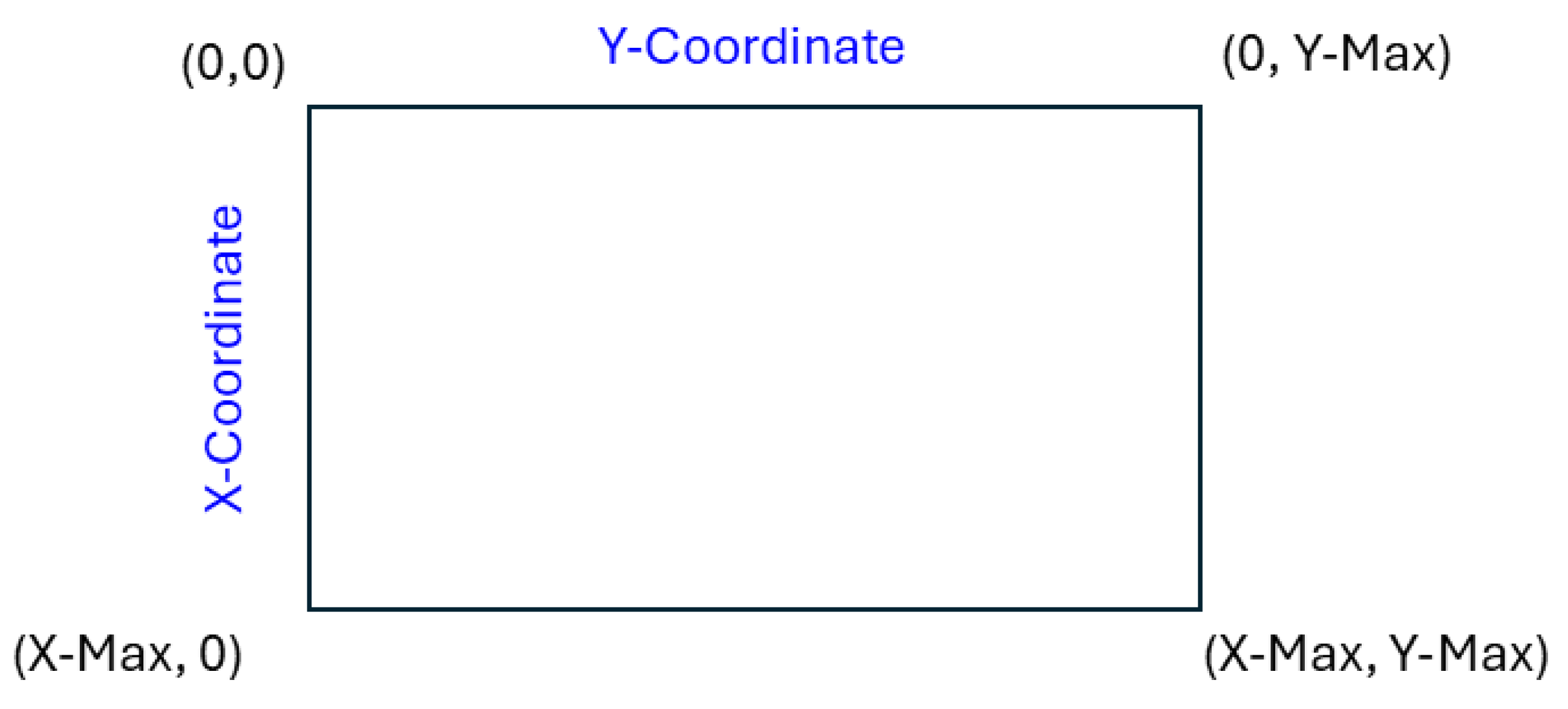
The coordinate system we have used for Mars is [X,Y], corresponding to row x column indexing. This aligns with the dimensions of an image file when viewed numerically.
We refer to Figure Table 4 for known mineral locations referenced in this study; these locations were originally sourced from [34]. We convert the [Y,X] coordinates provided by [34] into our [X,Y] format to ensure consistency and reproducibility. These locations serve as the source of the hyperspectral reference spectra used in the MRO CRISM Type Spectra Library for the specified minerals. In some cases, we rotated the unprojected TER-3 images by 180 degrees to match the orientation presented in [34]. We explicitly noted the rotations in the corresponding image descriptions for transparency and reproducibility, and Table 4 summarises the adjustments.
Figure 4.
Pixel coordinate system used in this study.
3.2. Data Preprocessing
We utilise two CRISM datasets in the TER format, taking the following issues into consideration:
- Summary product recalculation: We use summary products derived from specific spectral absorption features [8] to cluster minerals as summary products are designed to detect key mineral signatures. Although MTRDR images files include these summary products, our analysis identified discrepancies between the values contained within and their intended spectral formulas used to generate them [16,35]. Therefore, we use Targeted Empirical Record - version 3 (TER-3) files, which enable us to recalculate summary products from the original spectral measurements. TER-3 is a specific CRISM image type [35] that consists of un-projected hyperspectral observations that have been corrected for atmospheric and photometric effects for Mars.
- Spectral labelling: We use the MRO CRISM Type Spectra Library to label clusters, which provides reference spectra for each mineral, specifically, we use the Numerator from the library - the source of which is also from a pixel in a TER-3 image - where the mineral has been previously verified [47]. These spectra serve as ground truth references to support the identification of mineral clusters detected by the SOM model. Ideally, each pixel (numerator) would be normalised using a reference pixel (denominator) and the ratio used to calculate summary products. Whilst the library provides a denominator for each reference spectra, we did not adopt this approach due to uncertainty about reliably identifying a reference pixel in each TER-3 image. If done incorrectly, this could complicate comparisons between the summary products calculated from targeted TER-3 image files and library reference spectra. Spectra for each mineral contained within the library is converted into a summary product for direct comparison.
We applied a unified preprocessing pipeline to both datasets to ensure compatibility between the summary products and the reference spectra, consisting of the following steps (Figure 5, Step 2).
- We mask pixels that have a specific value of 65535 in any frame, as this indicates invalid or missing spectral data. These pixels are excluded from analysis, and summary products are not calculated for them.
- We compute summary products for each pixel from the unmasked pixels.
- We clip any summary product values below zero to zero. Although the formula for summary products does not specify a minimum bound. We refer to BD1750_2 in Equation (1), which can yield negative values, absorption features are inherently positive. This clipping approach is consistent with recommendations in the literature [34].
- We normalise all summary products to a range [0,1] to eliminate dimensional disparities and standardise inputs for the model.
Although normalisation of summary products (input features) to the [0,1] interval promotes consistency, it also overemphasises certain mineral signatures. Ideally, the inputs should be scaled with reference to a global range of summary product values, not local target regions. For example, if the maximum value of BD1750_2 in target regions "A" and "B" were 0.005 and 0.1, respectively. The local scaling would independently scale both maximums to 1, effectively treating them as equivalent. In contrast, global scaling performed across both regions would result in scaled values of 0.05 for region "A" and 1 for region "B". In this case, global scaling preserves the relative difference in absorption strength, maintaining the weaker BD1750_2 response in region "A" rather than inflating it to match region "B" under local scaling.
3.3. Unsupervised Machine Learning Framework
After processing the data, as shown in our framework (Figure 5), we apply K-means clustering to group pixels based on spectral similarity. Experimentally, we select the number of clusters such that the smallest cluster contains approximately ten percent of valid pixels in an image (Figure 5 - Step 3). For each training iteration (repeated "X" times), we randomly and equally sample from each cluster formed in Step 3 to generate a batch of "N" instances for a single SOM training update. This approach ensures that no single spectral group dominates the training set, maintaining diversity across iterations (Figure 5 - Step 4). Clustering before sampling mitigates redundancy in the training data, preventing premature neuron convergence and allowing the SOM to learn a more meaningful representation of the spectral space.
We use each instance in a training batch to sequentially train the SOM model. We then integrate the SOM output with the MRO CRISM Type Spectra Library to produce labelled mineral clusters, topology maps. We then provide an analysis of the minerals clustered through the framework (Figure 5 - Step 5).
Each neuron in our SOM model is associated with a 29-dimensional weight vector, corresponding to the summary products used as input features. We initialise these weight vectors with random values in a range [0,1], this assists with initial learning, as the summary products used as inputs are restricted to this range. Although this random initialisation is typically sufficient for model convergence, more structured initialisation methods could potentially accelerate learning and enhance clustering performance. We employ a competitive learning strategy based on the principles introduced by Kohonen [48] and extended to clustering tasks by Vesanto [25] to get a better organised topological map from the SOM. This involves a two-stage training process designed to first establish a rough global organisation and then refine local cluster distinctions.
Figure 5.
Flow diagram illustrating the progression from raw inputs to SOM model outputs.
- Stage 1- Rough Topological Organisation: In the initial stage, neurons are updated with a high learning rate and a large neighbourhood radius, facilitating a coarse topological structure that guides the model in later stages.
- Stage 2- Refinement: The learning rate progressively decays, and the neighbourhood radius shrinks, enabling the model to fine-tune and converge on subtle distinctions in mineral characteristics.
3.3.1. SOM Implementation
We enforce the initial organisation of the randomly initialised weights by 50 preliminary model training iterations before commencing formal training. We select the initial learning rate as and the radius for a SOM map. The initial learning rate and radius of updated neuron nodes gradually decrease.
The SOM model undergoes 1,000 iterations of formal training to cluster instances (Step 4 of Figure 5). We use 5,000 instances in each iteration, randomly but equally sampled from each cluster formed in Step 3 of Figure 5. The number of clusters formed during the pre-training instance clustering process may vary, but typically, around 20 clusters are generated, with the smallest cluster containing contain about 2000 instances. Over 1000 iterations, each instance in the smallest cluster is expected to be used for training approximately 125 times, or once every ten iterations, ensuring that small clusters are adequately represented and not overlooked by the SOM model during training.
We relied on heuristic estimates [46] to determine the SOM model dimensions (hyperparameters such as length and width) and did not delve into hyperparameter optimisation-due to a SOM’s topological organisation, which is tolerant of over-dimensioning by grouping similarly weighted neurons within - effectively forming a cluster of clusters. Our visual inspection of a neuron heatmap suggests that a 50×50 SOM is likely over-dimensioned, as there are often topological clusters of high correlation among many neurons. Nonetheless, the impact of moderate over-dimensioning appears minimal, as the SOM’s topological structure maintains meaningful organisation by grouping highly correlated neurons into hierarchical clusters. These can be further clustered by external algorithms or interpreted through visual inspection of the neuron heatmap. However, there are instances in which a 50×50 SOM was required to isolate a particular mineral, notably Epidote in target region FRT0000CBE5 (not shown in this paper). Therefore, under-dimensioning SOM, where distinct clusters cannot be effectively separated likely poses a greater risk than over-dimensioning, which primarily results in redundant but topologically organised clusters.
3.3.2. Cluster Labelling
In order to correlate the clusters with known mineral types, we compare the trained neuron weight vectors with processed reference spectra from the CRISM MRO Type Spectra Library. We compute the correlation scores by comparing the 29 normalised summary products of each neuron’s weight vector with the reference spectra. We assigned the neurons with higher correlation scores, indicating greater spectral similarity, with tentative mineral labels. This approach enables the partial labelling of unsupervised clusters, enhancing their interpretability without requiring training data.
3.3.3. Threshold for Mineral Confidence Levels
We focused on regions identified by the top five neurons with the highest correlation to the reference spectrum to assess the spatial distribution of a labelled mineral. These neurons generally exhibited strong spectral similarity, particularly in areas where the mineral was previously confirmed to exist. However, simply selecting the top five neurons can yield misleading results in regions where the mineral is not present. Therefore, we excluded neurons with low correlation scores, even if they ranked among the top five for a given mineral. In an attempt to refine and automate this process, we explored an alternative approach.
- Correlation Calculation: We calculate the correlation of all 2,500 neurons to each of the 31 mineral reference spectra in the CRISM MRO Type Spectra Library, resulting in 77,500 individual correlation values.
- Global Thresholding: The neurons are considered to have a high correlation to a mineral if their correlation exceeded the 95th percentile of all neurons. The median correlation value was also used as a threshold, with neurons correlating with the median being excluded from further consideration.
-
Z-Score Transformation: For each mineral, the correlation values to each neuron were converted to z-scores (for just that mineral). A neuron was deemed to belong to a mineral if:
- -
- The neuron had a high correlation with the mineral, and its z-score exceeded the mean z-score for that mineral across all neurons (indicating a strong and representative correlation).
- -
- Alternatively, if the mineral’s correlation to the neuron was low, the z-score had to exceed 2 to be considered relevant.
- Rationale for Approach: This method was adapted based on our observations that some minerals appeared to be widely distributed across a target region, while others were highly localised. The approach aimed to capture both scenarios by emphasising stronger correlations for widely distributed minerals and allowing for more flexibility with more isolated minerals.
Despite experimenting with this approach, we found that selecting the top five neurons was generally sufficient for most analyses, as our focus was on regions where the presence of specific minerals had already been reported. This method offered a straightforward yet effective way to associate SOM neuron weight vectors with known mineral signatures, delivering reliable results without the need for complex thresholding in most cases.
4. Results
We present four examples to demonstrate the ability of our framework, which utilises a SOM model to detect the spatial distribution of minerals on Mars and highlights its advantages for mineral exploration.
- A visual comparison of the SOM model’s ability to detect the spatial distribution of the mineral Illite with reference to the distribution identified by Viviano et al. [34].
- The SOM model’s ability to detect the specific location of the mineral Low-Ca Pyroxene, as previously identified by [34].
- An application of the SOM model’s topological structure to identify the presence of Mg-Carbonate on Mars in a previously unknown location.
- A qualitative review of the topological organisation of mineral groups within the SOM model neuron grid.
4.1. Mineral Classification
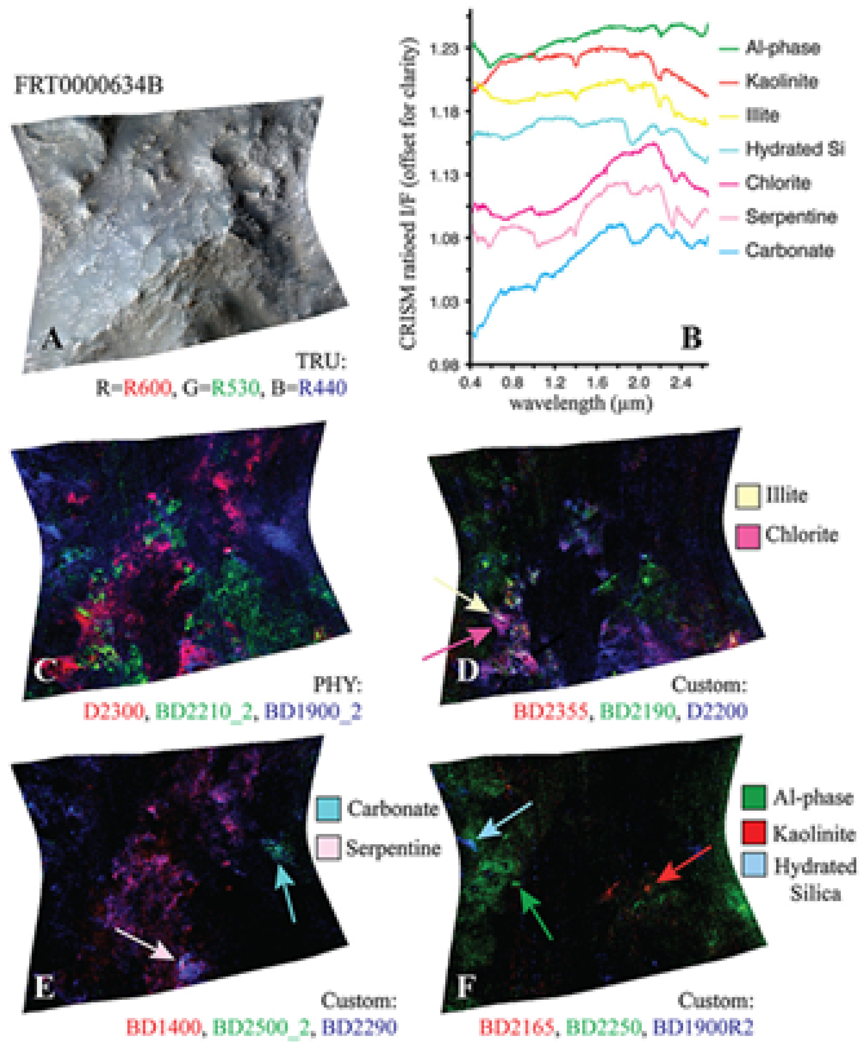
Figure A3 from the literature provides an opportunity to evaluate the SOM model’s ability to identify the spatial distribution of Martian minerals. Figure 6a shows the spatial distribution of the mineral Illite as identified by the SOM model along with our attempt to replicate image D of Figure A3. Although Illite is intended to appear as pale yellow, in our overlay (Figure 6a), it appears to render as a colour closer to pale pink (a consequence of local scaling). The overlay reveals a strong alignment between the highlighted pale pink areas and the clusters identified by the SOM model - particularly clusters 0 and 2.
Although the polygonal boundary includes broad pale pink zones - especially within cluster 0 - in Figure 6a, the SOM model appears more precise in its identification of Illite. Hence, Figure 6b highlights with white pixels the specific regions where the SOM model detected Illite. This emphasises the model’s accuracy in pinpointing even thin strips of Illite which is not demonstrated by the broader polygon based representation.
Table 1 [34] identifies Low-Ca Pyroxene as present at the coordinate location [174, 528] within a 9×9 pixel area in target region FRT000064D9. This location appears to visually align with the neon aqua-blue regions in Image H from Figure A2, offering an additional opportunity to evaluate the SOM models ability to identify the spatial distribution of a mineral. Although this region is not explicitly labelled in Image H from Figure A2, its association with Low-Ca Pyroxene is visually supported by the coordinate reference and Martian surface features. We note that Figure A2 is map-projected, while the coordinate reference is not.
Figure 7a shows the region identified by the SOM model, overlaid with our replication of Image H from Figure A2. The highlighted area corresponds to the top five neurons most strongly correlated with the processed MRO CRISM Type Spectra Library sample for Low-Ca Pyroxene.
Although the SOM model correctly identifies the target region with the top 5 neurons, this is likely an example of over-dimensioning the SOM Model. Regarding Figure 8, many neurons in the top left hand corner of the SOM model are correlated with the mineral, and ideally, should be clustered to a smaller number of neurons. Figure 7b shows the identified spatial distribution if the top 50 neurons are used. Overall, the SOM model appears to effectively capture the spatial distribution of Low-Ca Pyroxene and topologically organises those pixels within the map.
4.2. SOM Model Structure and Mineral Organization
Fe-Olivine appears to be widespread in the target region FRT00003E12, with a substantial majority of SOM neurons exhibiting a strong correlation to the mineral. Rather than assessing the correlation of each neuron to a particular mineral, Figure 9a considers the hit rate of each neuron, this reveals a very distinct topological cluster with a relatively low hit rate in the upper-left corner of the SOM.
The only mineral mapped to this distinct region is Mg-Carbonate. While Mg-Carbonate shares activity in OLINDEX3 and BD1300 with Fe-Olivine, it additionally exhibits strong responsiveness to BD2290 and several other summary products which Fe-Olivine does not. This spectral distinction is echoed in the SOM structure, which topologically separates Mg-Carbonate into a unique cluster of neurons, mirroring the spectral separation intentionally embedded into our overlay design. As shown in Figure 9b, the SOM has clustered Mg-Carbonate into the top left quadrant and away from Fe-Olivine, which is mapped to the top right quadrant (not shown).
Figure 6.
Comparison of two overlays for FRT0000634B indicating Illite detection using a SOM model. Both images are rotated 180 degrees to align with Image D from Figure A3 and have a resolution of 390×640 pixels, with the X-axis oriented vertically to align with the image rows.
Figure 6.
Comparison of two overlays for FRT0000634B indicating Illite detection using a SOM model. Both images are rotated 180 degrees to align with Image D from Figure A3 and have a resolution of 390×640 pixels, with the X-axis oriented vertically to align with the image rows.
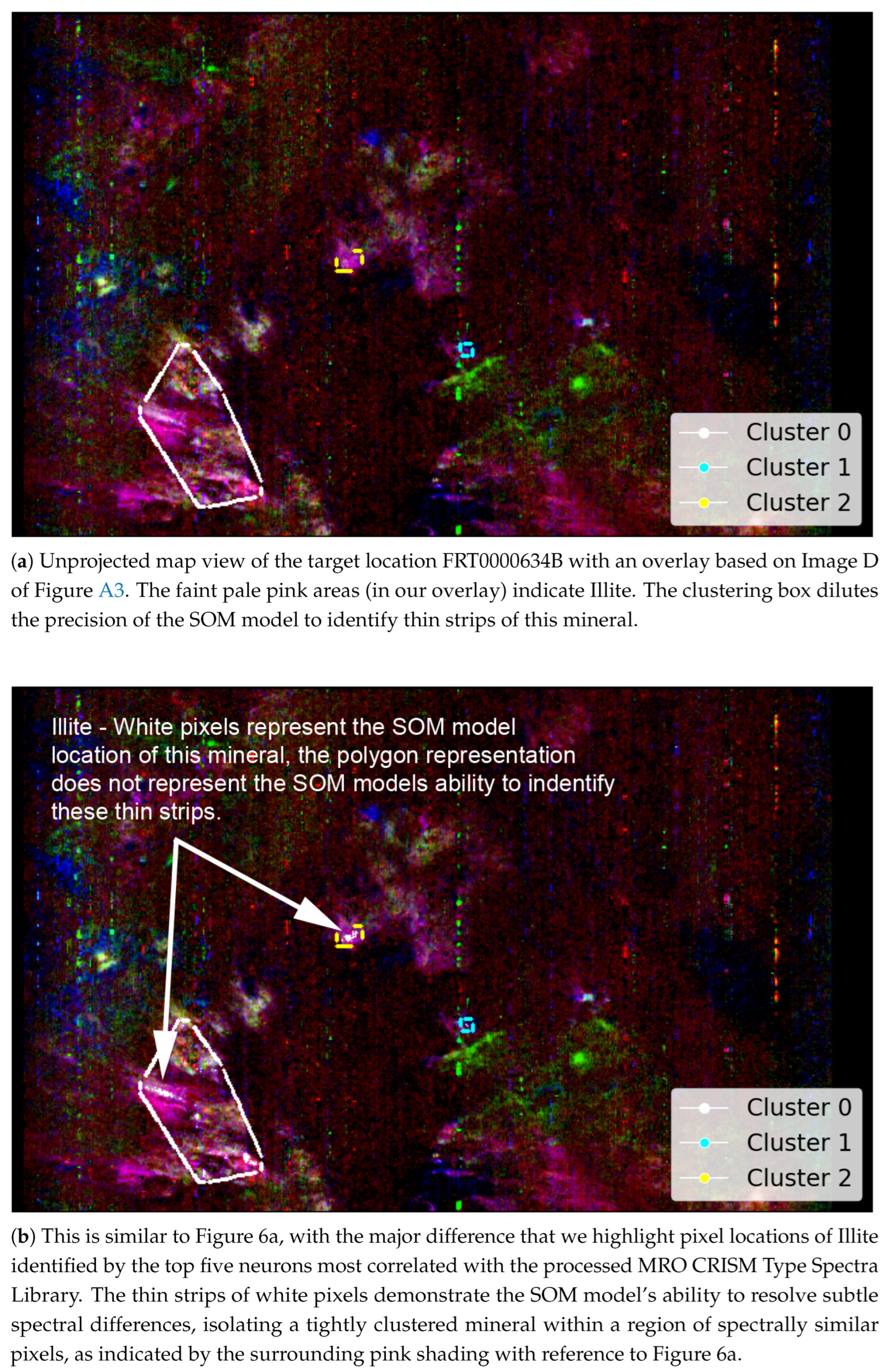
Figure 7.
Unprojected map views of target location FRT000064D9, showing Low-Ca Pyroxene detection based on neurons correlated with the MRO CRISM Type Spectra Library. All images are rotated 180 degrees to align with Image H from Figure A2 and have a resolution of 480×640 pixels, with the X-axis oriented vertically to match image rows.
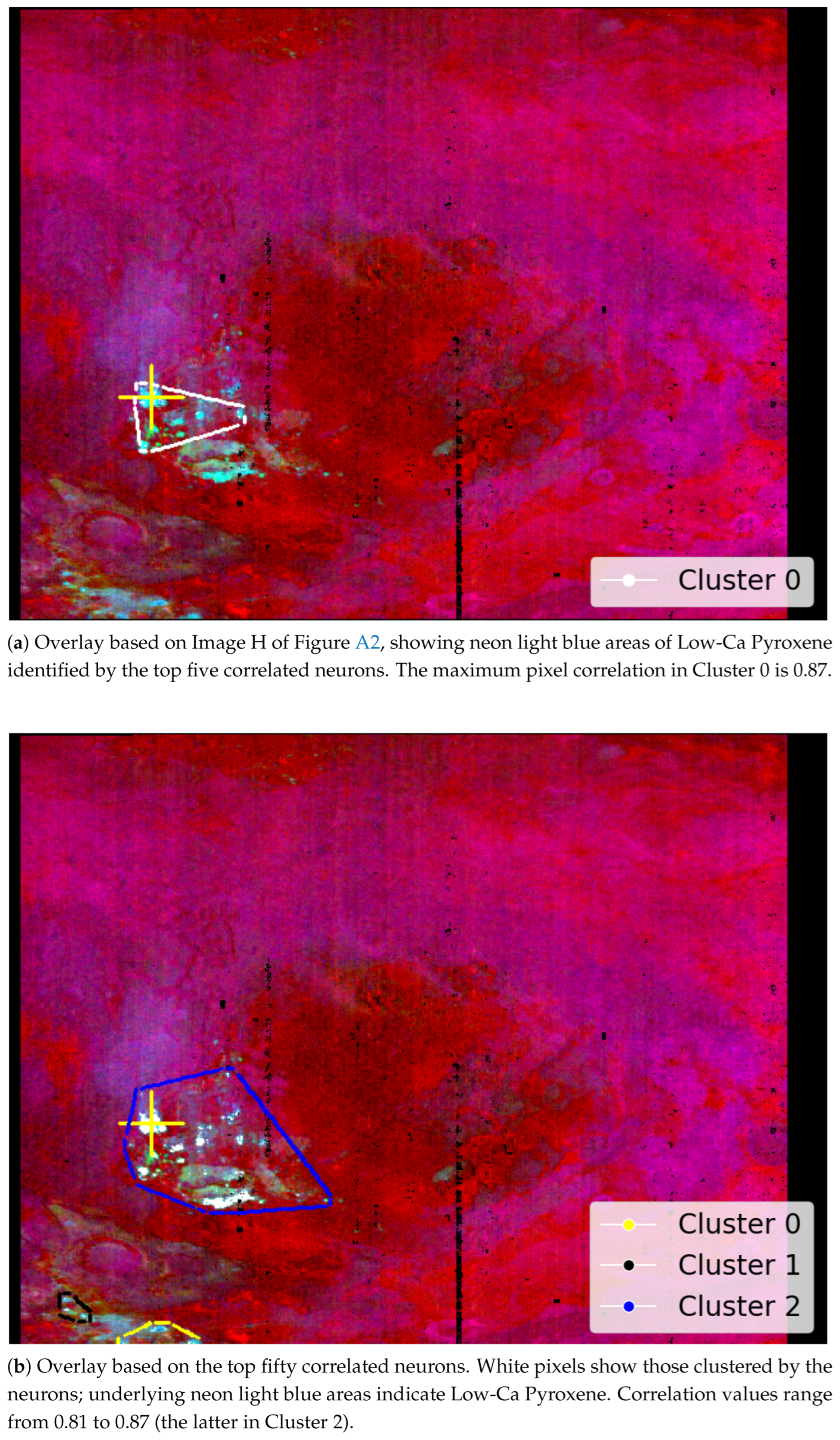
Figure 8.
Heatmap of SOM neurons showing correlation to Low-Ca Pyroxene in region FRT000064D9, based on comparison with the MRO CRISM Type Spectra Library. Each pixel in this image corresponds to a neuron in the SOM model, starting with neuron 0 at the top-left corner [0,0] and ending with neuron 2499 at the bottom-right corner [50,50], comprising a total of 2500 neurons.
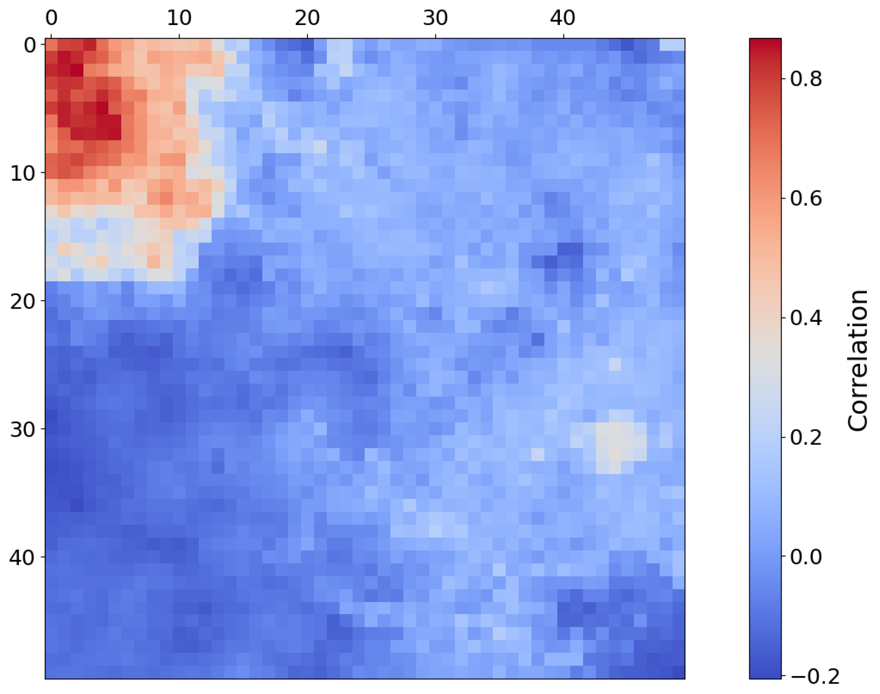
Figure 9.
Neuron hit count and correlation map for region FRT00003E12. Each pixel in these images corresponds to a neuron in the SOM model, starting with neuron 0 at the top-left corner [0,0] and ending with neuron 2499 at the bottom-right corner [50,50], comprising a total of 2500 neurons.
Figure 9.
Neuron hit count and correlation map for region FRT00003E12. Each pixel in these images corresponds to a neuron in the SOM model, starting with neuron 0 at the top-left corner [0,0] and ending with neuron 2499 at the bottom-right corner [50,50], comprising a total of 2500 neurons.
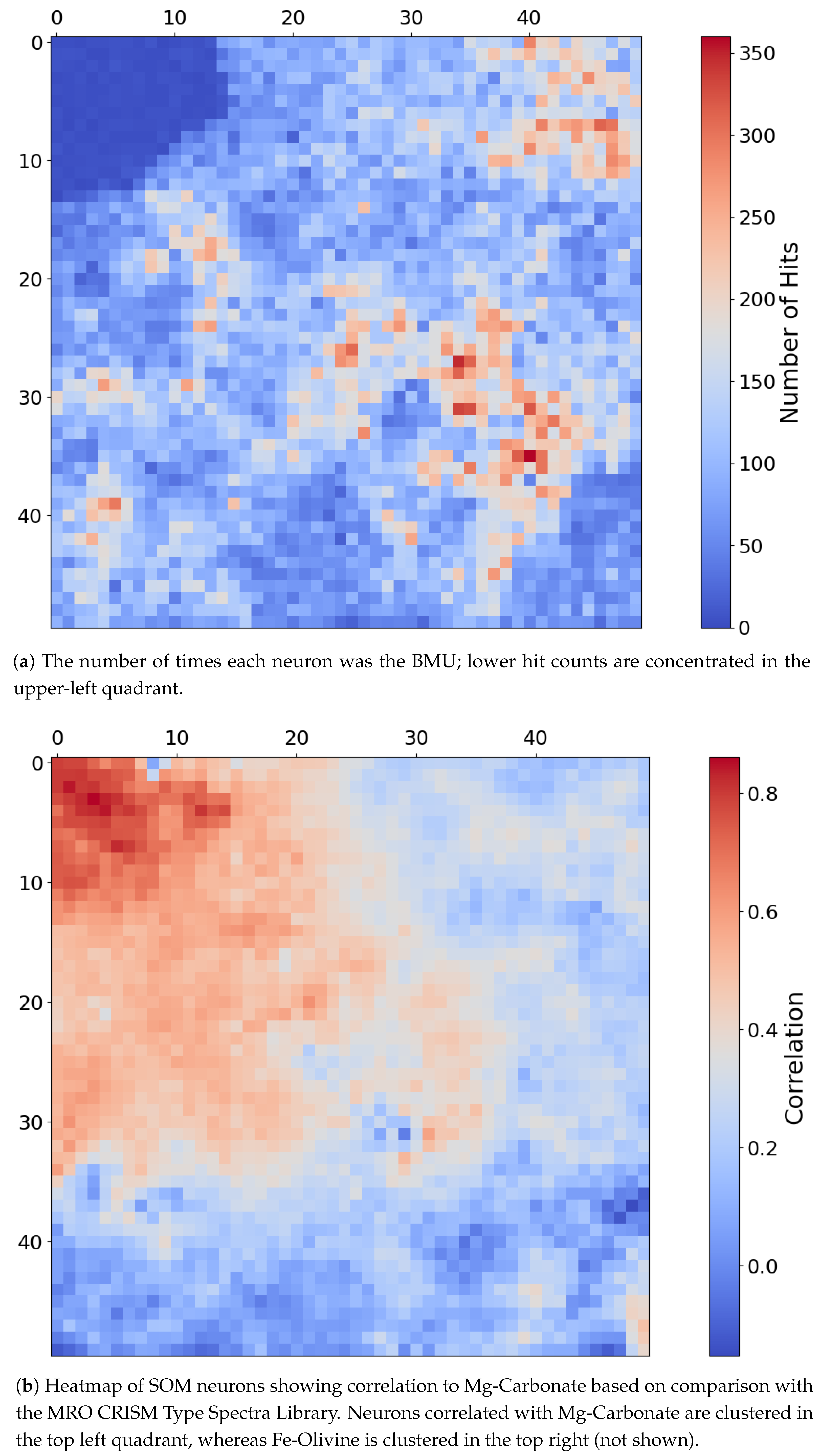
The extended moderate neuron correlation to Mg-Carbonate in Figure 9b is likely due to the extensive presence of Fe-Olivine in this target region (FRT00003E12) and the fact that Mg-Carbonate is responsive to many of the same summary products as Fe-Olivine. We demonstrate the isolated nature of Mg-Carbonate in target region FRT00003E12. Figure 10 presents the CR2 overlay recommended by Viviano et al. [34] to visualise the presence of this mineral. It confirms the identification of Mg-Carbonate or at least some other mineral that is distinctly different to Fe-Olivine in the same spatial context. The detection of this isolated mineral was made possible by the topological relations that are preserved by the SOM model and one of the many available topological views.
Figure 13(a) shows the inferred distribution of minerals mapped for target region FRT0000634B, where each neuron is following the application of our Thresholding criterion based on correlation strength and z-score. A distinct pattern is revealed in which minerals localise around the corners and edges of the SOM model.
Figure 11 shows the frequency with which each mineral group was detected in the four corners of the SOM model, revealing a hierarchical pattern in the clustering.
- The top-left corner of Figure 11 is notably sparse in Phyllosilicate minerals, which are primarily mapped to neurons in opposing corners.
- Sulfates and Ices (the latter of which there are only two instances of in the MRO CRISM Type Spectra Library) are more prevalent in the upper regions of the SOM model, with ices absent from the bottom corners.
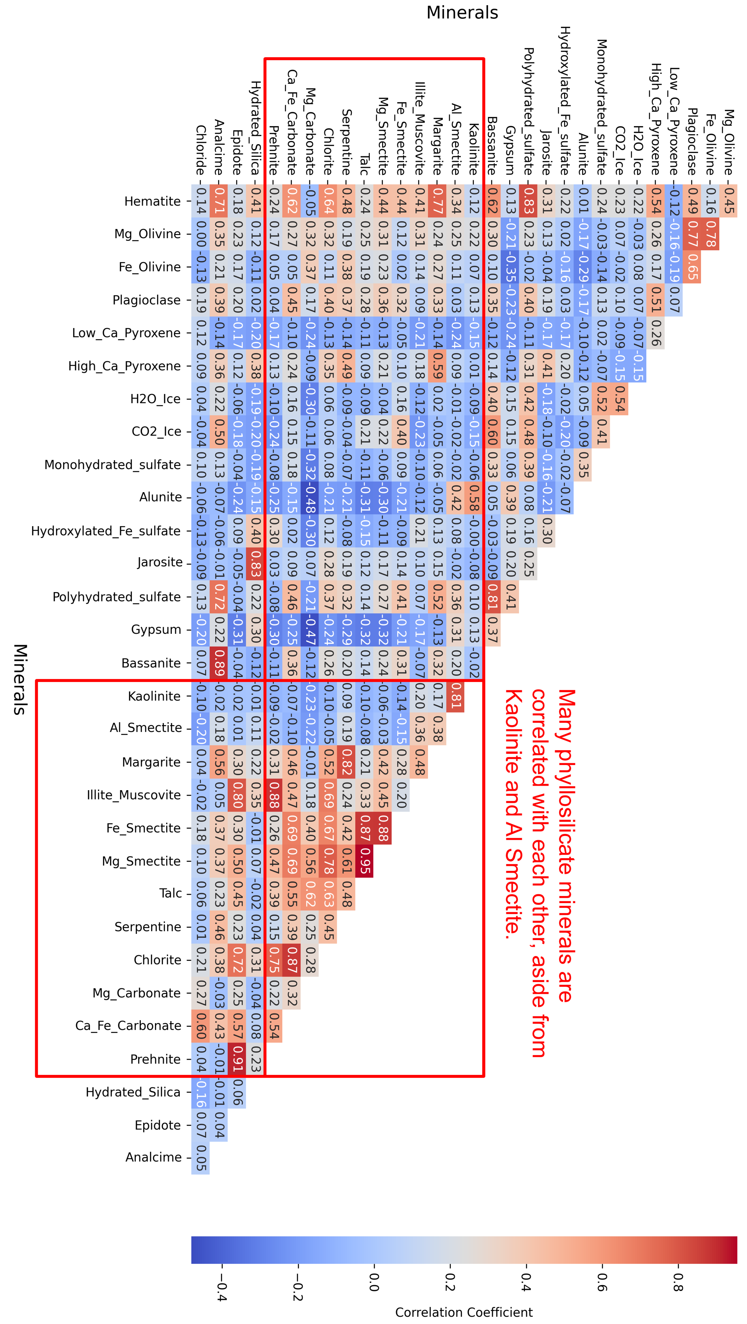
We examine a correlation heatmap of the minerals from the processed MRO CRISM Type Spectra Library to better understand the structure and organisation (refer to Figure 12) and note there is a similar pattern to the SOM model:
- Phyllosilicates exhibit high intra-group correlation, except for Kaolinite and Al-Smectite, which are mostly negatively correlated with their peers.
- Ices are consistently only correlated with Sulfates.
As phyllosilicates are highly correlated (and thus why some neurons are mapped to multiple minerals), neurons activated by these minerals tend to draw in neighbouring neurons, causing the phyllosilicates to cluster together. This clustering occurs throughout the SOM model, except in the top-left corner where phyllosilicates are sparse, refer to Figure 11. Similarly, the SOM model appears to group Ices and Sulfates along the top of the map.
Further examination reveals that Kaolinite is negatively correlated with its group and is mapped to neurons primarily in the top-right corner, away from other phyllosilicates. Additionally, Al-Smectite, another phyllosilicate negatively correlated with its group (and positively correlated with Kaolinite), is also mapped primarily in the top-right and bottom-left corners and is also separated from the majority of phyllosilicates, which are in the bottom right corner. By way of example for this target region, Figure 13(b) and Figure 13(d) shows the correlation of SOM model neurons to Al-Smectite and Talc respectively, whilst both phyllosilicate minerals the scaled summary products for Al-Smectite and Talc are negatively correlated and the SOM model has topologically separated the two minerals.
If it were not for the negatively correlated Kaolinite and Al-Smectite to their group, the entire top region of this SOM model maybe mostly free of phyllosilicate minerals, highlighting the separation of groups and alignment with the inherent patterns in the data which, when trying to identify an unknown mineral, this topology may offer clues as to which mineral group the unknown mineral belongs to.
Figure 10.
Unprojected map view of FRT00003E12 using the recommended CR2 overlay, highlighting potential Mg-Carbonate rich areas. Unlike other images, no individual pixels are marked in this overlay. The yellow regions are a direct result of the overlay and represent isolated and distinct mineral clustering in this area. The SOM delineated regions were generated by selecting the top 15 neurons — those with a correlation exceeding 0.8 to the reference spectra, which are the highest correlating neurons located in the top-left corner of the neuron heatmap.
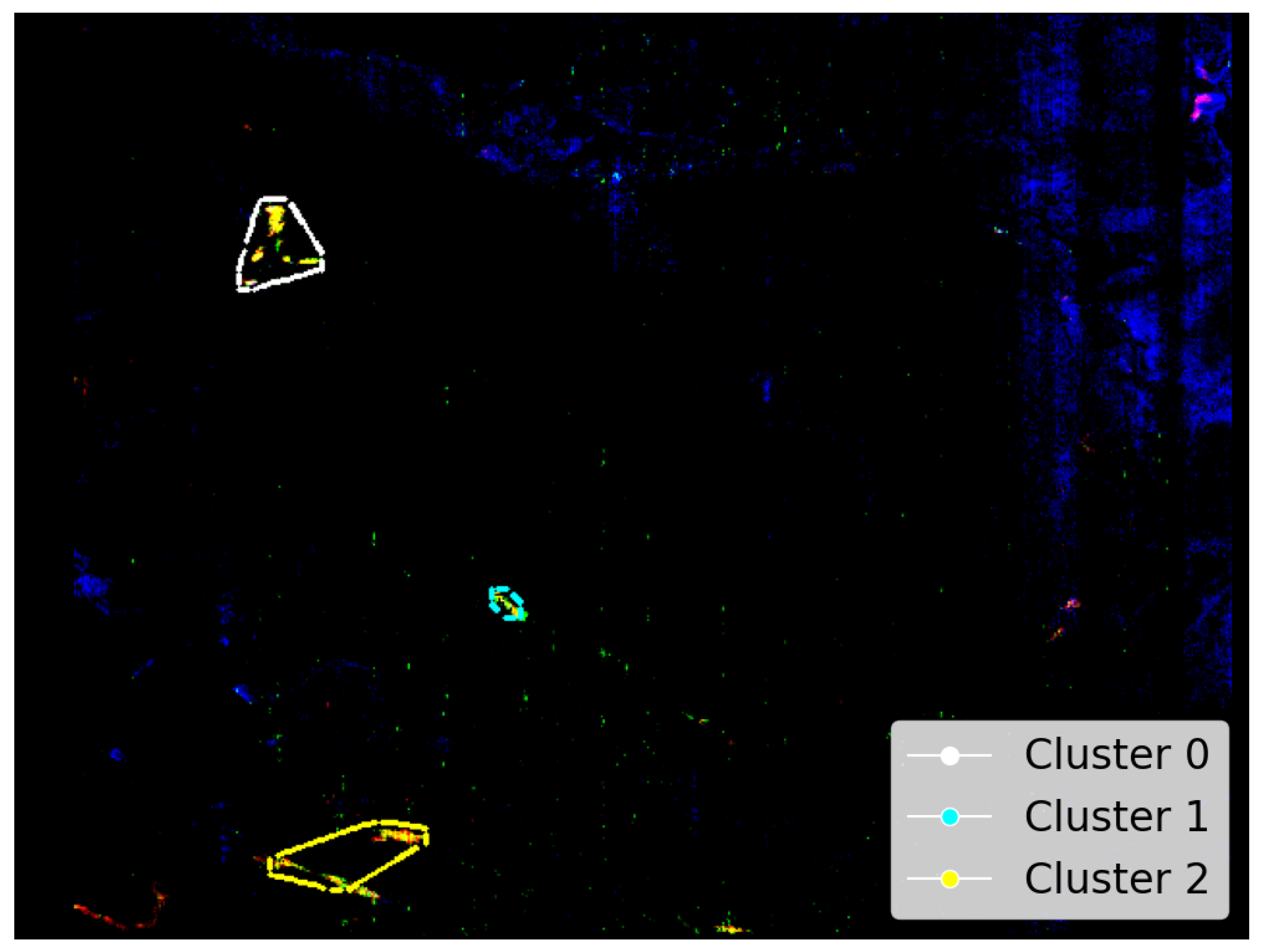
Figure 11.
An analysis of the mineral categories associated with the neurons located at each corner of the SOM model for target area FRT0000634B.
Figure 11.
An analysis of the mineral categories associated with the neurons located at each corner of the SOM model for target area FRT0000634B.
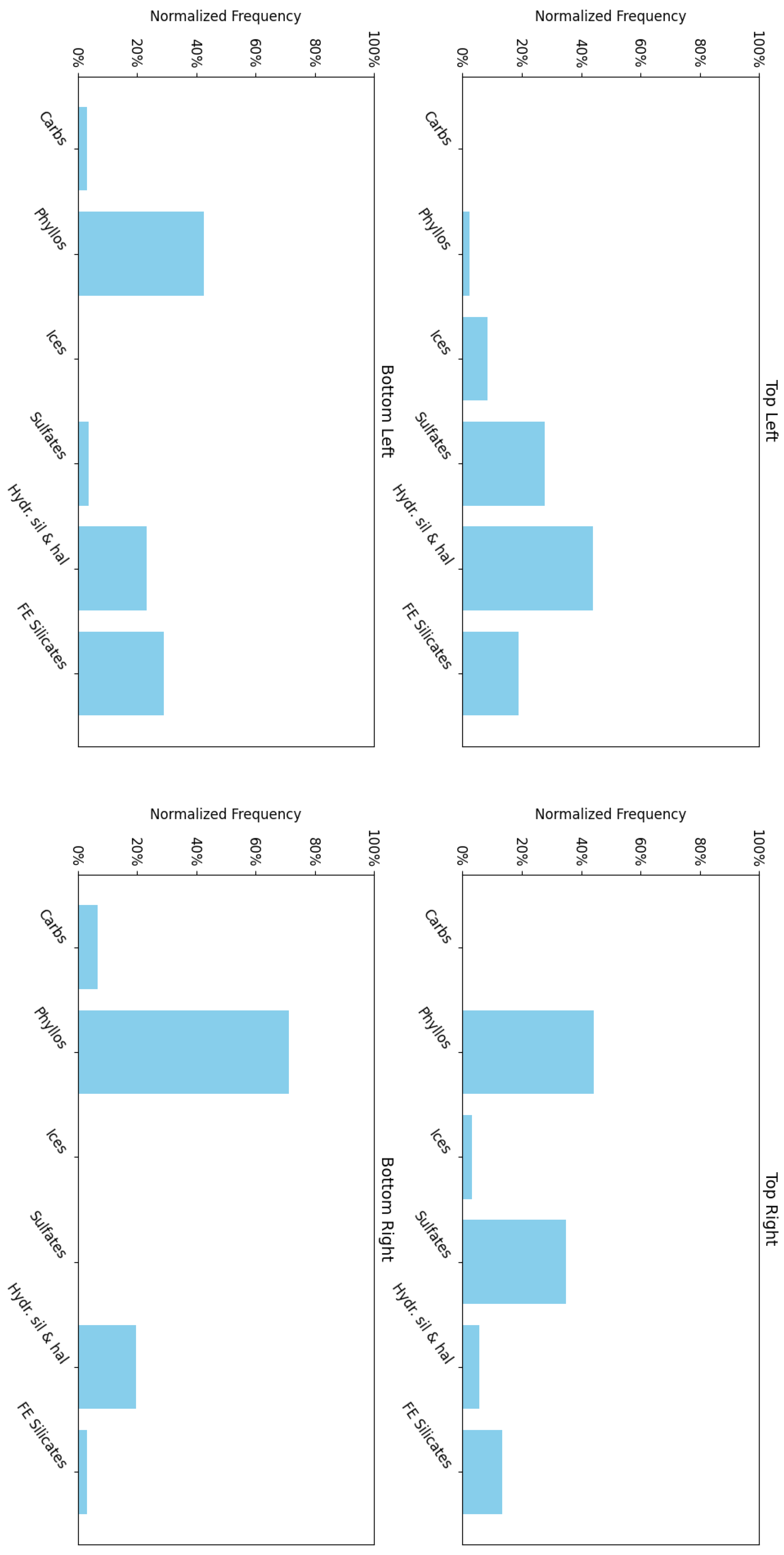
Figure 12.
Correlation heatmap of processed MRO Library Minerals.
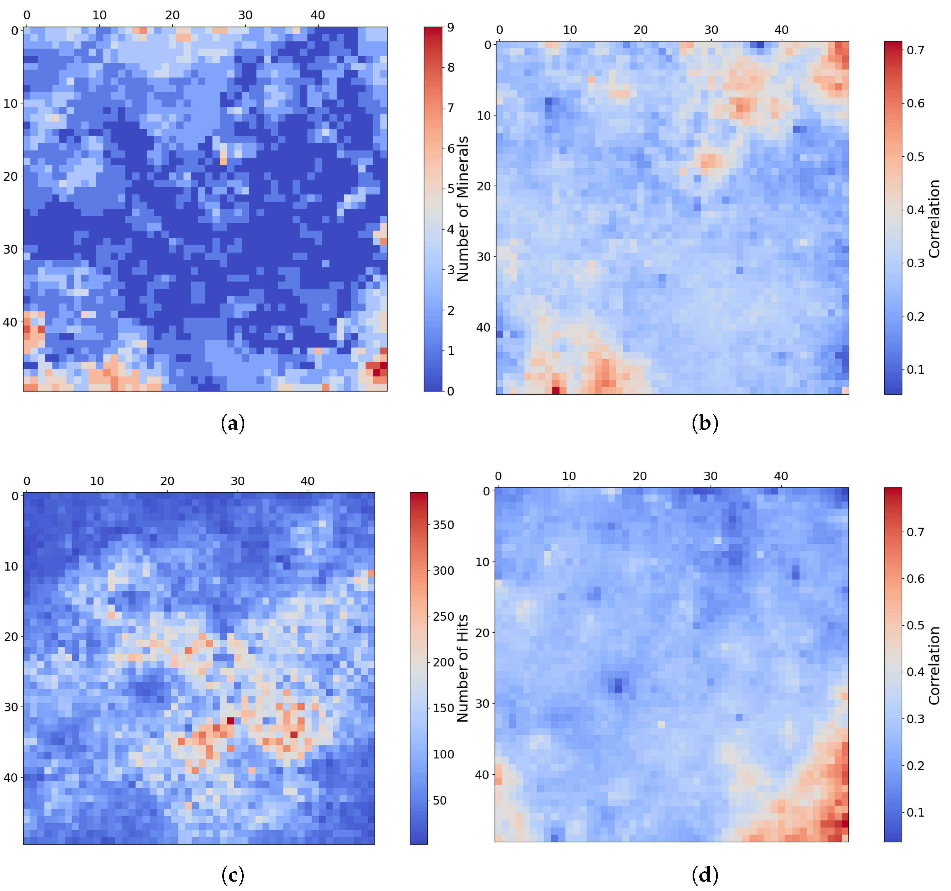
We also examined the frequency with which neurons were activated and notice an inverse relationship between the neurons that likely represent a mineral (Figure 13(a)) and those that receive the most hits (Figure 13(c)). This may indicate that many pixels contain mixed data, making it difficult to reliably identify anything unique. We believe this is an important observation and a key reason for selecting samples from K-means clustered data when training the SOM model as described. By doing so, we can better represent groups (with few instances) that are likely to contain minerals, as opposed to the majority of instances, which appear to be uninformative and potentially redundant.
Figure 13.
Mineral mapping, correlation, and hit rate for each neuron in target region FRT0000634B. Each pixel in these images corresponds to a neuron in the SOM model, starting with neuron 0 at the top-left corner [0,0] and ending with neuron 2499 at the bottom-right corner [50,50], comprising a total of 2500 neurons. (a) The number of minerals mapped to each neuron. Neurons with multiple mapped minerals suggest a high degree of feature correlation among those mineral groups. (b) Neuron correlation to Al-Smectite. (c) The number of times each neuron was identified as the BMU. The SOM model appears to cluster uninformative neurons near the centre of the map, where we observe the highest hit counts. (d) Neuron correlation to Talc.
4.3. K-Means Clustering
Compared to the SOM model, K-Means clustering is significantly more efficient at clustering instances. However, K-Means lacks the topological organisation capabilities of a SOM model - a feature that proved critical when identifying Mg-Carbonate in target region FRT00003E12. This topological structure enables neighbouring neurons to group similar instances and appears to result in a more focused and specialised clustering. Across various cluster/neuron sizes, the SOM model:
- Demonstrates stable clustering of instances identified as Mg-Carbonate, with both SOM training iterations appearing to show reduced variation in clustering assignments. Notably, the SOM results remain close to the mean and well within the confidence interval generated from 30 independent K-Means trials (see Figure 14(a)).
- Generates tighter clusters, as indicated by a mean weighted distance that is consistently and significantly lower than that of K-Means (see Figure 14(b)).
- Allocates more neurons to represent distinct and unique instances, capturing greater detail (see Figure 14(c)).
Figure 14.
Comparison of clustering performance between 30 independent K-Means trials and two SOM model series (SOM and SOM ) across varying cluster/neuron counts. We present the mean performance in solid lines and the shaded confidence interval for K-Means represents the 5th and 95th percentiles across the 30 trials. We compute the error metrics using only clusters or neurons with a correlation greater than 0.75 to Mg-Carbonate spectra from the MRO CRISM Type Spectra Library. (a) Total number of instances assigned to clusters (K-Means) or neurons (SOM) identified as representing Mg-Carbonate. (b) Mean weighted distance, indicating the compactness and cohesion of clusters (K-Means) or neurons (SOM). (c) Total number of clusters (K-Means) or neurons (SOM) matching Mg-Carbonate across tested model sizes. (d) The execution time for SOM across tested model sizes.
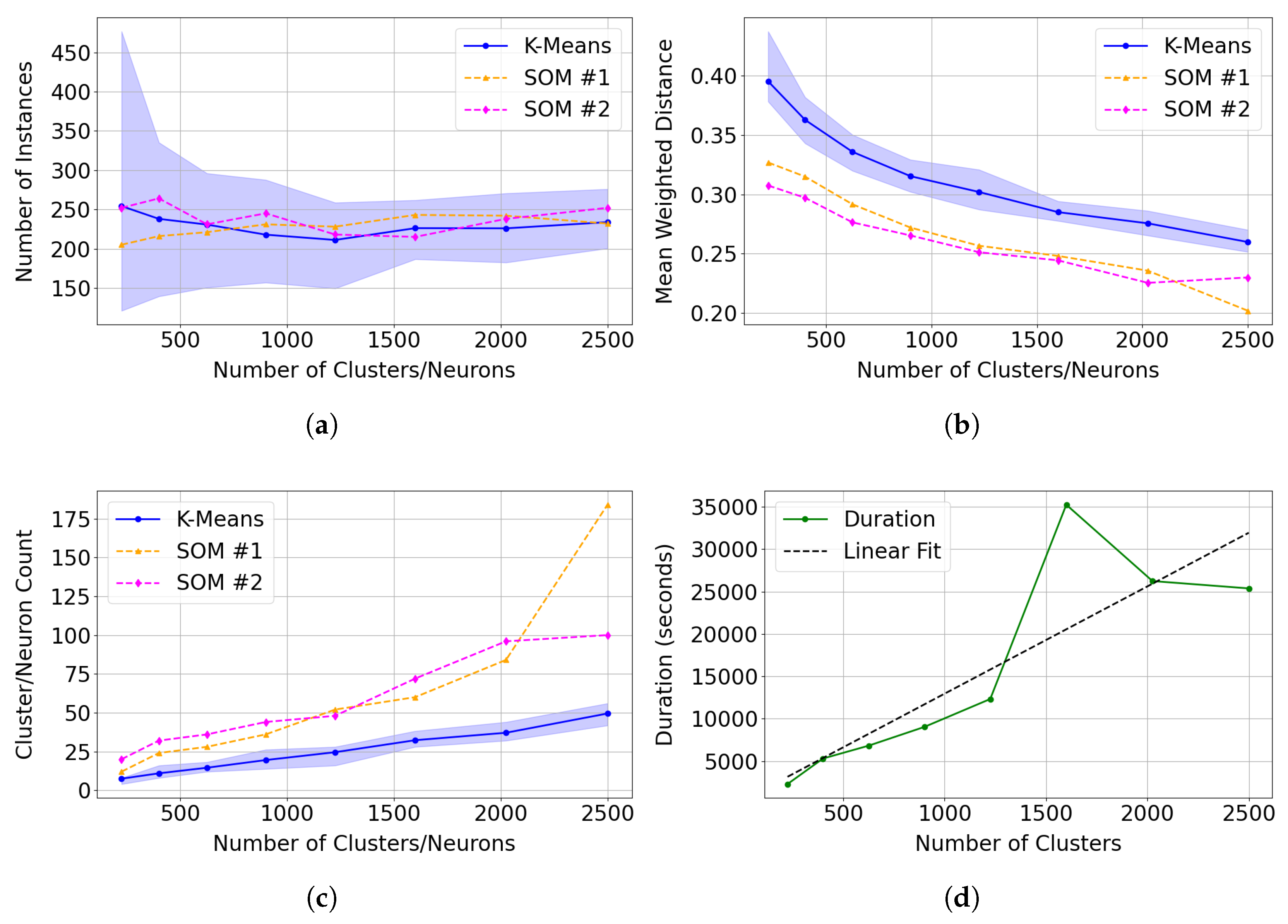
The execution time (runtime) of the two models is not directly comparable, as the SOM model includes a greater number of hyperparameters, which can significantly affect training time. In this study, we fixed the training at 1,000 batches of 5,000 sequentially updated instances per batch, an arguably excessive configuration. A key factor contributing to the extended runtime of the SOM is its requirement for sequential updating, which prevents parallel processing. All models were developed and executed using PyCharm Community Edition 2024.3.4 with Python 3.12.4, on a Windows 11 Pro system equipped with a 12th Generation Intel Core i7 processor (12 physical cores, 20 threads) and 32 GB of RAM. Under this architecture, model run times did not consistently scale with model size; in some cases, larger SOMs completed faster than smaller ones. This counterintuitive behaviour is likely due to external factors influencing performance during long training periods. For the models referred to as SOM in Figure 14, the training times as specified in Table 1 and displayed in Figure 14(d).
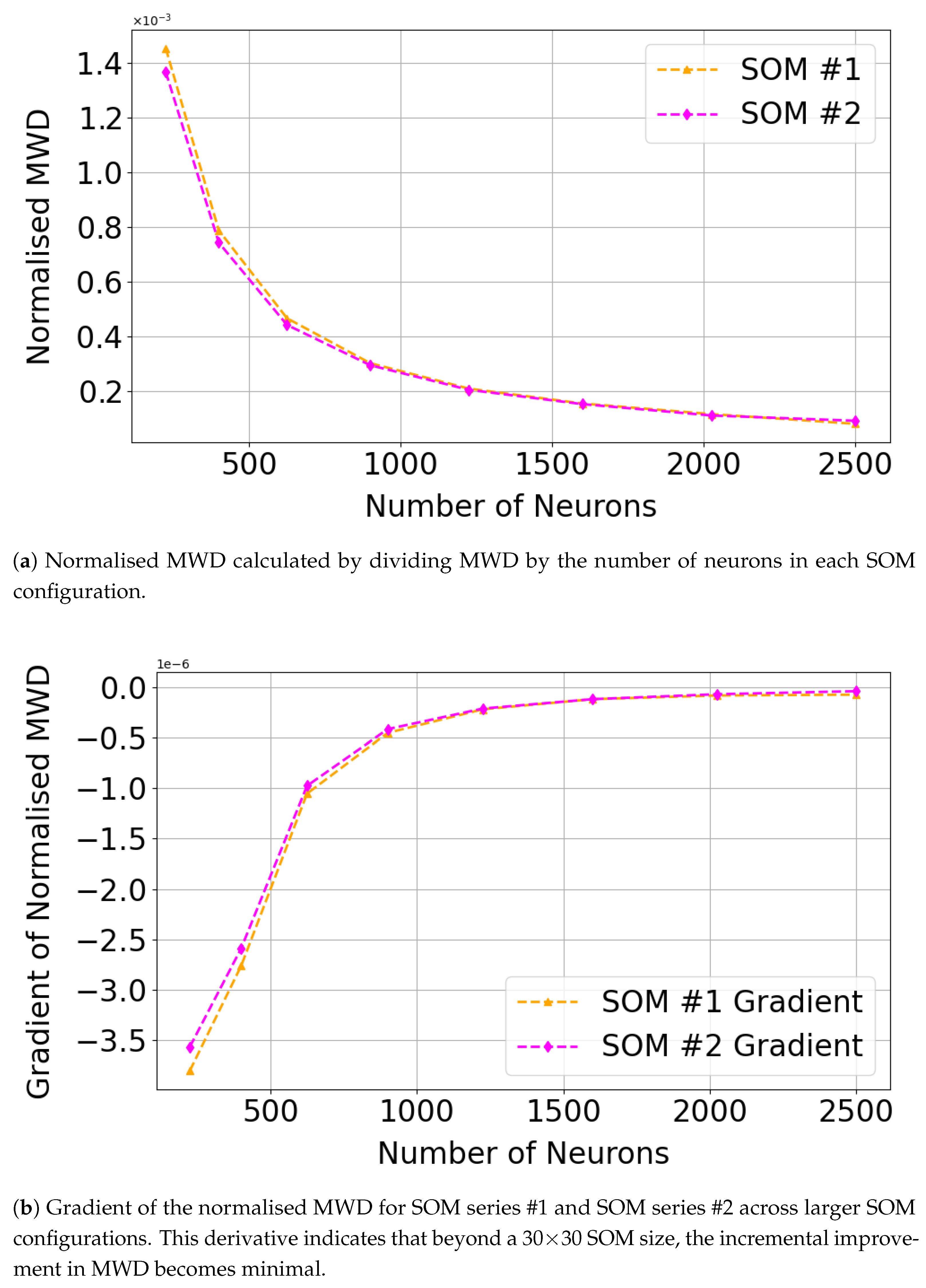
As shown in Figure 15 and Table 2 and Table 3, a SOM size of 30×30 (900 neurons) appears sufficient to cluster Mg-Carbonate in this region as the improvement in normalised Mean Weighted Distance (MWD) is minimal beyond this point. We note that the numerical gradient of the normalised MWD flattens beyond this point. The target image contained 460×640 pixels, of which 273,001 were valid (i.e., not equal to 65535 in any layer), out of a total of 307,200. This suggests that the commonly used heuristic of neurons, where N is the number of valid pixels (see Section 3.3.1) may be excessive in this context.
Figure 15.
Performance trends in SOM clustering with larger SOM configurations, based on normalised MWD and its gradient.
Figure 15.
Performance trends in SOM clustering with larger SOM configurations, based on normalised MWD and its gradient.
5. Discussion
This research demonstrates that unsupervised models can identify geologically meaningful patterns in processed hyperspectral data, and the resulting clusters can be labeled by referencing spectral libraries such as the MRO CRISM Type Spectra Library. This helps to bridge a gap in extraterrestrial mineral exploration and identification where validation data is limited, such as Mars. Therefore, we introduced a tailored feature selection strategy that condenses high-dimensional spectral data into a more manageable and informative representation using summary products. We identified and documented specific inconsistencies between the CRISM MTRDR image files [16] and the CRISM DPSIS [35]. Highlighting these discrepancies contributes to improving data quality and the reliability of hyperspectral remote sensing for Martian exploration.
Our findings demonstrate that the SOM model is well-suited for mapping mineralogical features. It not only detects regions associated with target minerals but also provides a topological structure that enhances the interpretation of mineral relationships. The analysis of target area FRT00003E12 highlighted the model’s ability to isolate Mg-Carbonate as a distinct mineral cluster within a region overwhelmingly dominated by Fe-/Mg-Olivine (see Section 4.2). This result underscores the value of pre-clustering, which ensures a diverse selection of spectral inputs during training and exposes the SOM to isolated spectral data, enabling it to recognise the topological separation of Mg-Carbonate. Although the SOM does not consistently isolate individual pixels with absolute precision, it reliably captures coherent mineralogical regions that align closely with established reference maps. We also identified a potential pattern where unique spectra representing minerals tend to be clustered by neurons located toward the edges of the SOM and exhibit relatively low hit rates. These observations may be useful for identifying unknown minerals in future research.
In this study, we identified several areas where further research is needed to enhance the accuracy and reliability of mineral detection and spatial distribution analysis on Mars using CRISM hyperspectral data:
- This study utilised the set of summary products outlined in Figure A1, however significant spectral overlap remains among many minerals, which limits the ability of clustering algorithms to differentiate between compositionally similar but distinct mineral types. While the MTRDR dataset includes approximately 60 summary product bands, we have only validated, corrected and recalculated 29 of these. Expanding the feature set to include additional summary products may improve mineral discrimination, but each new feature must be validated due to the discrepancies identified with precomputed summary products within MTRDR files and the intended spectral features. These discrepancies appear to exist in both directions - MTRDR files contain formula errors when compared to the CRISM DPSIS documentation, while in other cases, the formulas in the CRISM DPSIS do not accurately reflect updated or enhanced outputs found in the MTRDR files [16,35].
- An expert review of the formulae to compute summary products is warranted as current versions rely on conflicting or overlapping definitions from multiple sources, for example, in some instances, the same summary product has a different formula specified in [34] compared to [35]. Although this research addressed several known issues, uncertainty remains whether some summary products accurately capture the intended spectral features in the first instance. This ambiguity risks leading clustering algorithms to identify misleading or spurious patterns, ultimately undermining the reliability of the results.
- Ideally, a machine learning approach to deriving summary products by automatically identifying key spectral features may be a preferred approach compared to expert review. Unlike traditional, expert-driven methods, which are time-consuming, subjective, and may miss complex patterns, machine learning methods should be capable of generating summary products that overcome these shortcomings.
- Normalising hyperspectral data using a representative reference (or "bland") pixel within each target region has the potential to enhance diagnostic absorption features, this technique is widely used in CRISM-based analyses [34,47]. In this study, summary products were derived directly from unnormalised TER-3 hyperspectral data. While this approach simplifies preprocessing, it may reduce the clarity of absorption features and hinder mineral differentiation. Future work should explore automated methods to reliably identify representative bland pixels within each region to facilitate normalisation.
- For each target region, summary product values were scaled locally, i.e., normalised between 0 and 1 based on the minimum and maximum values within each individual target region. While this method is effective for within-region clustering, it introduces inconsistencies when comparing results across multiple regions. For instance, two regions may appear to contain similar mineral signatures when scaled locally, but global scaling could reveal significant differences. Additionally, the color representation of mineral associations, as per Figure 9 in [34], becomes inconsistent across regions due to the relative nature of local scaling. A more rigorous approach would involve applying global normalisation using consistent reference values, though this would require the construction of a comprehensive global database of summary product statistics. Summary products derived from hyperspectral data from the MRO CRISM Type Spectra Library should be scaled according to the same global limits.
- Our results show that the SOM model organises into stable topological patterns, often clustering similar mineral types in adjacent nodes. This raises the possibility of accelerating SOM model training by initialising weights based on an informed prior structure. Further investigation into pre-initialisation techniques may improve training efficiency and output quality.
- A promising avenue for future work involves training a global SOM model exclusively on verified mineral spectra, independent of any specific region. This "Master SOM model" could then be deployed to new Martian sites for rapid classification and mapping. Such a model would enhance consistency, reduce preprocessing time, and allow for more direct comparisons between studies and across target areas. Due to the global nature of this approach, normalised hyperspectral data would be required before deriving summary products.
- A critical challenge in planetary mineralogy is the identification of pixels with spectral profiles that do not closely match any known hyperspectral samples. Developing a systematic approach to detect and flag distinct but unknown spectra signatures might be important for discovering new or unknown mineral types.
The following table and map indicates the target regions referred to, the location of specific minerals and adjustments made to image files:

Table 4.
The table outlines the target regions and, where applicable, the original [X, Y] pixel coordinates of mineral locations shown in all satellite and overlay images used in this research. These coordinates correspond to positions prior to any image rotation. For more details, refer to 3.1.
Table 4.
The table outlines the target regions and, where applicable, the original [X, Y] pixel coordinates of mineral locations shown in all satellite and overlay images used in this research. These coordinates correspond to positions prior to any image rotation. For more details, refer to 3.1.
| Mineral | Figure | Target Region | Original X | Original Y | Rotated |
|---|---|---|---|---|---|
| Illite | 6a | FRT0000634B | NA | NA | YES |
| Illite | 6b | FRT0000634B | NA | NA | YES |
| Low-Ca Pyroxene | 7a | FRT000064D9 | 174 | 528 | YES |
| Low-Ca Pyroxene | 7b | FRT000064D9 | 174 | 528 | YES |
| Mg-Carbonate | 10 | FRT00003E12 | NA | NA | NO |
Mars surface image view showing the targeted regions referred to:
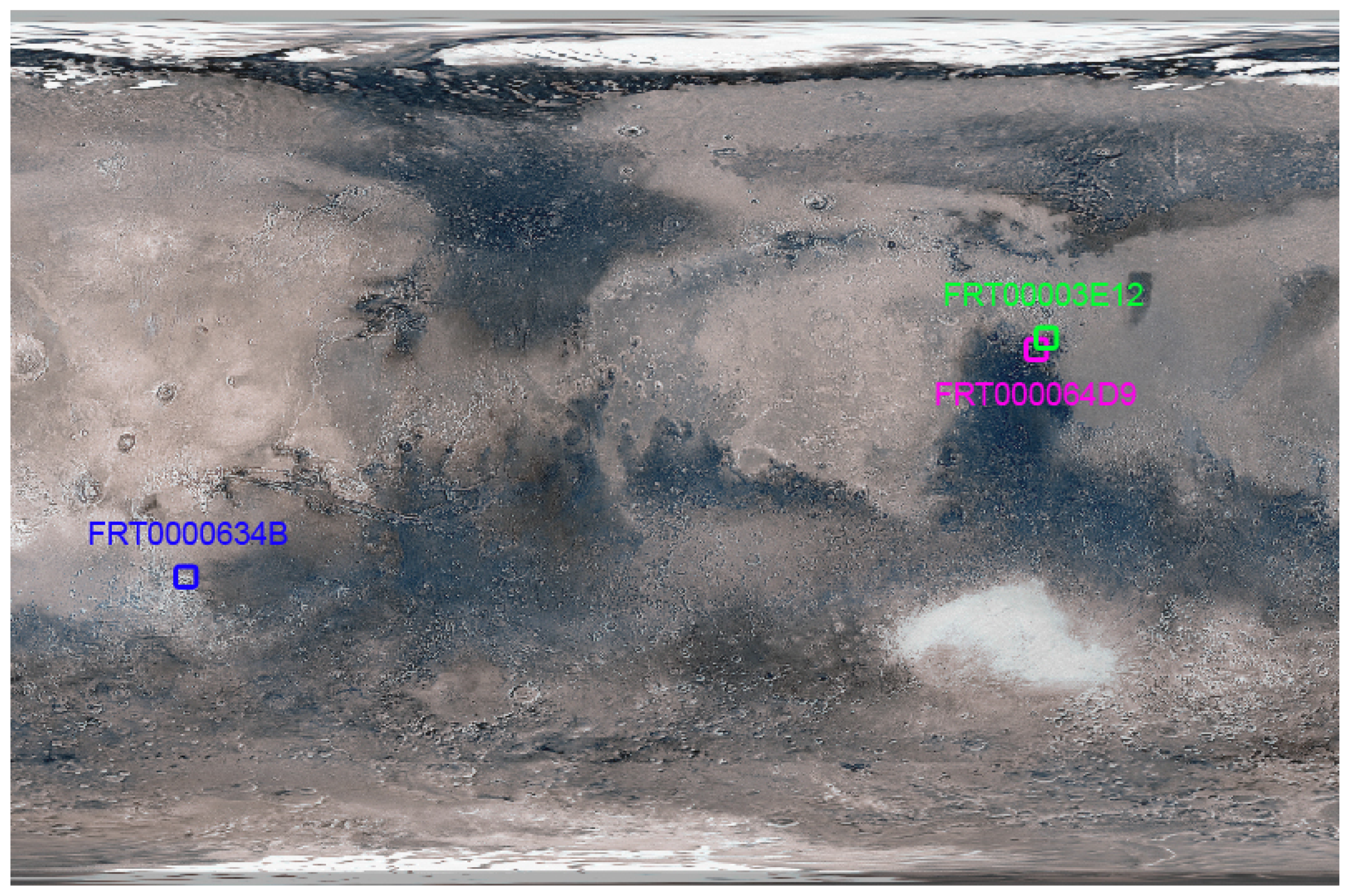
Figure 16.
Global view of Mars showing enlarged and approximate locations of the target regions referred to.
Figure 16.
Global view of Mars showing enlarged and approximate locations of the target regions referred to.
6. Conclusions
This study advances the understanding of Martian mineral detection by demonstrating how unsupervised clustering, specifically using a SOM model guided by spectral libraries and informed feature selection, can reveal both the spatial distribution and hierarchical organisation of mineral deposits from remote sensing hyperspectral data. Our investigation revealed that compared to K-means clustering, the SOM model allocates more resources to unique spectra, producing tighter and more distinct clusters. This improvement appears to stem from a unique property of the SOM model - its ability to preserve topological relationships, which helps distinguish groups with similar spectral signatures and enables the creation of additional visual overlays for mineral detection. Although more computationally intensive, the SOM model offers significantly richer structural and visual detail, making it a valuable tool for future mineral classification and mapping efforts on Mars.
Python code, including visual overlay generation and topological SOM analysis is available on GitHub at: https://github.com/sydney-machine-learning/mars-minerals/releases/tag/v2.0.0
Author Contributions
T. Lovelock was responsible for feature selection, development of the Self-Organising Map (SOM) model, data acquisition and preprocessing, and the implementation of all Python code. He also drafted and co-authored the technical sections of the manuscript, including the methodology, results, and related analyses. R. Chandra contributed to the conceptualisation of the study, project supervision, experimental design, data analysis, and editing of the final manuscript draft. All authors have read and agreed to the published version of the manuscript.
Funding
This research received no external funding.
Institutional Review Board Statement
In this section, you should add the Institutional Review Board Statement and approval number, if relevant to your study. You might choose to exclude this statement if the study did not require ethical approval. Please note that the Editorial Office might ask you for further information. Please add “The study was conducted in accordance with the Declaration of Helsinki, and approved by the Institutional Review Board (or Ethics Committee) of NAME OF INSTITUTE (protocol code XXX and date of approval).” for studies involving humans. OR “The animal study protocol was approved by the Institutional Review Board (or Ethics Committee) of NAME OF INSTITUTE (protocol code XXX and date of approval).” for studies involving animals. OR “Ethical review and approval were waived for this study due to REASON (please provide a detailed justification).” OR “Not applicable” for studies not involving humans or animals.
Data Availability Statement
Original CRISM TER-3 data, processed summary product outputs and SOM model outputs is available for download via Zenodo:
- Target region FRT00003E12 - https://zenodo.org/records/16397494
- Target region FRT000064D9 - https://zenodo.org/records/16397520
- Target region FRT0000634B - https://zenodo.org/records/16397583
Python code, including visual overlay generation and topological SOM analysis is 683
available on GitHub at: https://github.com/sydney-machine-learning/mars-minerals/ 684
releases/tag/v2.0.0
Acknowledgments
We thank Haoyu Sun from UNSW Sydney for earlier contributions. We thank Ehsan Farahbakhsh from the University of Sydney. During the preparation of this study, the authors used ChatGPT to assist with some phrasing refinements, the generation of some figure and table captions, and the re-formatting of figures, tables, and equations per MDPI guidelines. The authors have reviewed and edited the output and take full responsibility for the content of this publication.
Conflicts of Interest
The authors declare no conflicts of interest.
Abbreviations
The following abbreviations are used in this manuscript:
| BMU | Best Matching Unit |
| CNN | Convolutional Neural Networks |
| CRISM | Compact Reconnaissance Imaging Spectrometer for Mars |
| DBSCAN | Density-Based Spatial Clustering of Applications with Noise |
| DPSIS | Data Product Summary Image Specification |
| EDR | Experiment Data Record |
| ICA | Independent Component Analysis |
| LMM | Linear Mixing Models |
| MNF | Minimum Noise Fraction |
| MRO | Mars Reconnaissance Orbiter |
| MTRDR | Map-Projected Targeted Reduced Data Record (CRISM) |
| MWD | Mean Weighted Distance |
| PCA | Principal Component Analysis |
| SOM | Self-Organising Map |
| TER | Targeted Empirical Record |
| TER-3 | Targeted Empirical Record version 3 |
| TRDR | Targeted Reduced Data Record |
| VNIR | Visible-to-Near-Infrared |
Appendix A. Visualise Mineral Locations
The figures and captions which follow are reproduced from [34].
Figure A1.
Summary product sensitivity matrices for each type spectra class (A-F). The top set of rows of each class show the response of analog laboratory material and the bottom set of rows show the corresponding response of CRISM MICA type spectra for each spectral parameter (columns). Each parameter is linearly scaled and has a fixed lower stretch limit of zero (black indicates a band depth at or below zero) and an upper limit of the highest response of the distribution (white). To the right of each matrix is the representative browse product RGB(s) (see Table 2 [34] for abbreviations) for that class set. Figure and caption reproduced from [34].
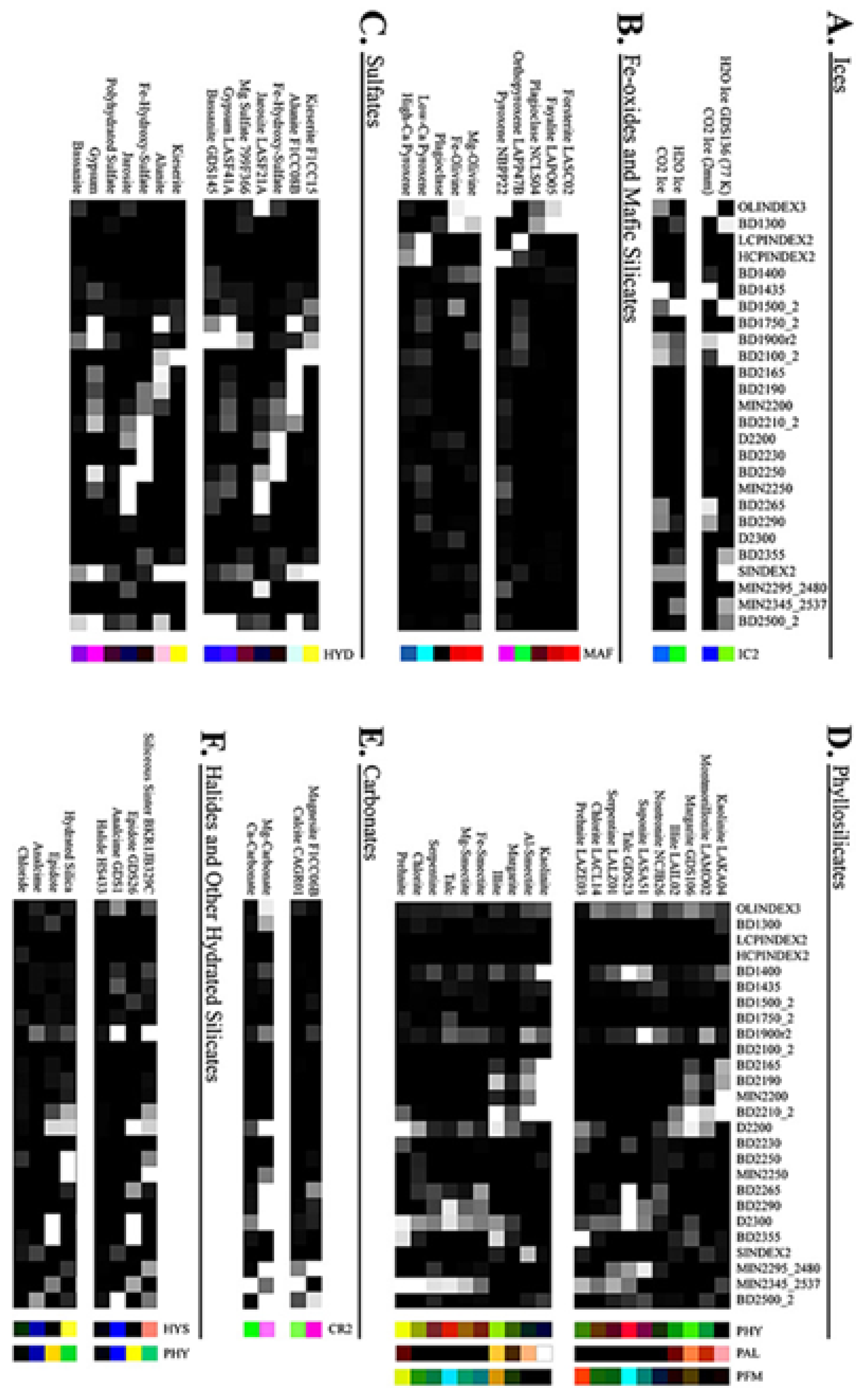
Figure A2.
A detailed example of summary and browse product development. The top row shows (a) CRISM MTRDR scene FRT0000B385 in false color stepped through (b) the old HYD browse product with a "global" stretch applied, (c) the same HYD product with the new "local" stretch applied, (d) the new parameter formulations for the revised HYD product, and (e) the new HYD product after noise filtering results. Figure A2b–e include a zoom-up box of a small region illustrating fine-scale changes that occur with improved stretching logic, refined parameter formulations, and noise filtering. The bottom row shows (f) CRISM MTRDR scene FRT000064D9 in false color stepped through (g) the old MAF browse product with global stretch applied, (h) the new MAF product with local stretch and noise filtering, and (i) extracted and ratioed CRISM I/F spectra from a particular location in this scene (white arrow, Figure A2h) and comparable laboratory spectra (RELAB) of high-Ca pyroxene (HCP) material. The old HCPINDEX displays no detection for this material (Figure A2g, blue channel), whereas the new HCPINDEX2 shows a strong detection of HCP (Figure A2h, blue channel). Figure and caption reproduced from [34].
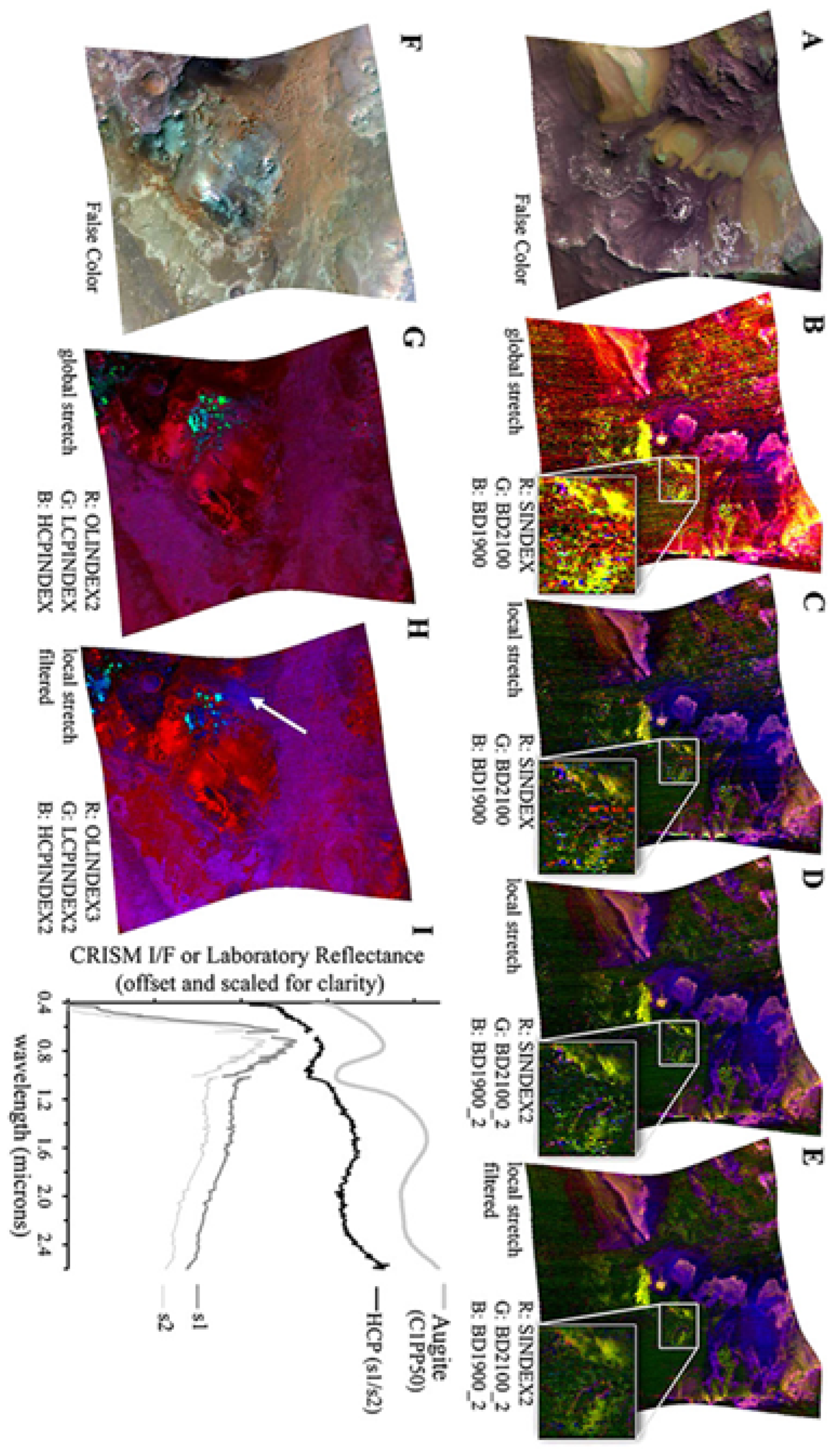
Figure A3.
A particularly diverse CRISM scene (FRT0000634B) revealing the utility of new summary product formulations. Although (a) the VNIR color stretch of this scene is somewhat homogenous, there are at least (b) seven type spectra represented in the image (locations of extracted spectra shown in subsequent panels with arrows). While (c) the standard PHY browse product reveals some hydroxylated silicate diversity, (d-f) custom combinations of new summary products are able to visually distinguish subtle spectral differences in the scene. Figure and caption reproduced from [34].
Appendix B. Summary Products
Table A1 presents the 29 recalculated CRISM summary products used in this study.
Table A1.
Summary product identifiers.
| OLINDEX3 | BD1300 | LCPINDEX2 | HCPINDEX2 |
|---|---|---|---|
| BD1400 | BD1435 | BD1500_2 | BD1750_2 |
| BD1900_2 | BD1900R2 | BD2100_2 | BD2165 |
| BD2190 | MIN2200 | BD2210_2 | D2200 |
| BD2230 | BD2250 | MIN2250 | BD2265 |
| BD2290 | D2300 | BD2355 | SINDEX2 |
| MIN2295_2480 | MIN2345_2537 | BD2500_2 | CINDEX2 |
| R3920 |
With reference to the CRISM DPSIS [35], the following corrections were applied either to align with the summary product outputs contained in the MTRDR files or to amend discrepancies in published summary products that did not conform to the DPSIS definitions, as discussed on the PDS Geosciences Node Community when MTRDR summary products could not be replicated [16].
- OLINDEX3 - The following kernel widths are used R1210:7, R1250:7, R1263:7, R1276:7, R1330:7 anchored at R1750:7 and R1862:7. The parameter is calculated as 0.1 × RB1210 + 0.1 × RB1250 + 0.2 × RB1263 + 0.2 × RB1276 + 0.4 × RB1330.
- HCPINDEX2 - The anchor points are R1690:7 and R2530:7, the parameter is calculated as 0.1 × RB2120 + 0.1 × RB2140 + 0.15 × RB2230 + 0.3 × RB2250 + 0.2 × RB2430 + 0.15 × RB2460
- BD1900R2 - A kernel width of 5 is used for the anchor bands R1850 and R2060.
- BD2100_2 - The kernel width of R2250:3 was used in place of R2250:5.
- MIN2200 - The kernel width of R2210:3 is used in place of R2120:3
- BD2230 - The kernel width R2235:3 is used in place of R2230:3
- BD2265 - The kernel width R2340:5 is used in place of R2295:5.
- R3920 is not specifically a summary product but is recommended by [34] for the IC2 Browse Product and was calculated using a kernel width of 5.
Appendix C. SOM Updates
The decay , learning rate and radius update functions used in our SOM models were:
The initial parameters for a SOM model were chosen to be and . These initial parameters ensure that a strong topological organisation occurs during the early stages of training. As recommended in the literature, an initial radius that is half of the largest dimension of the array is recommended [48], in this case a radius of 25 results in half of all neurons in the model being updated for each sequentially trained instance. Furthermore, an initial learning rate of 0.5 causes neuron weights to change rapidly. As the radius and learning rate decrease over time, the long-term impact of large initial values is mitigated, however, starting values that are too small can cause the SOM model to get stuck in a "metastable" configuration [48] preventing the SOM from learning and achieving meaningful topological organisation which the model may not recover from in subsequent learning. The value of in equation A1 was chosen to ensure that approximately 25% or 250 iterations of formal training had a radius less than 1, meaning 75% or approximately 750 iterations of the training involved updating the neurons around the BMU.
Appendix D. Data
With reference to the GitHub repository linked in the Data Availability Statement (Section 6), all results can be reproduced using the original CRISM TER-3 data by following the steps outlined below. Alternatively, both the CRISM TER-3 data and corresponding SOM outputs for the target regions analysed in this study are available for direct download from Zenodo, as also detailed in Section 6. The following steps (Appendix D - Appendix F) outline how to reproduce the results using our Python code and the original CRISM TER-3 data for a selected target region.
To begin, navigate to the MRO_Spectra_Library_Conversion folder and run the script CRISM_Replication_Library.py to process MRO CRISM Spectra Library Data.
Appendix D.1. Download CRISM TER-3 Image Files for a Target Region
Follow these steps to download the necessary CRISM TER-3 data for a specific region:
- In Step 1, select TER as the product type.
- In Step 2, define the target region by entering the appropriate Product ID such as FRT00003E12* for target region FRT00003E12.
- Review the search results.
-
Download all files containing "if" in the file name such asfrt0000cbe5_07_if166j_ter3.img.
After downloading the TER-3 data, follow these steps to convert the data into summary products:
- Consolidate all downloaded TER-3 files into a single folder. There should be an img (500+ mb), lbl and hdr file in the same folder.
-
Open the script CRISM_Spectral_Conversion.py located in theCRISM_Spectral_Conversion folder.
- Specify the path to the TER-3 .img file and set the desired output directory in the script.
- Execute the script.
Note: This process may take several hours to complete.
Appendix E. SOM
To train the SOM, follow the steps below. Summary product data must first be prepared by either generating it according to the procedure outlined in Appendix D or by using the preprocessed summary product files provided for a target region (see the Data Availability Statement in Section 6).
- Open the script som_training.py located in the SOM_Training folder.
- Set the path to the .h5 file which contains preprocessed summary products for the target region..
- Configure the SOM training parameters as necessary.
- Run the script to train the SOM.
Note: This process may take many hours for a 50×50 SOM with 1,000 iterations. However, training can be paused and resumed thanks to built-in functionality within the SOM class (as defined in som_class.py). The class accepts the inputs int_iter and int_weights, which allow training to resume from a specific iteration (int_iter) using the corresponding set of neuron weight vectors (int_weights). During training, the model is automatically saved at every 10th iteration.
Appendix F. Visualise Mineral Locations
The following steps outline the process for visualising the spatial distribution of specific minerals on the Martian surface. SOM data must first be prepared either by generating it using the procedure described in Appendix E, or by using the provided SOM output files for a target region (see the Data Availability Statement in Section 6).
- Open the script Layer_Visuals.py located in the SOM_Analysis folder.
- Specify the relevant data sources (including the original TER-3 image file - required for False views), which should be familiar from previous steps.
- Under the section Identify Spatial Distribution of a Specific Mineral, configure the settings for your analysis.
- The output will be a false-color or custom image displaying the identified spatial distribution of the nominated mineral on the Martian surface and target pixel location if you specify such a target.
Appendix F.1. SOM Hierarchical Analysis
For hierarchical analysis of the SOM model, perform the following steps:
- Open the script SOM_analysis.py located in the SOM_Analysis folder.
- Specify the relevant data sources from the previous steps (excluding the original TER-3 image file and summary product outputs contained in the h5 file).
- Run the script to perform a comprehensive topological analysis of the SOM model.
Appendix F.2. K-Means Comparison
To perform a K-Means comparison, follow these steps:
- Ensure the SOM model is trained before running this process, as the inputs reshaped_data_loc and reshaped_locations_loc are generated during the SOM training.
- Open the script kmeans.py located in the KMeans folder.
- Specify the relevant data locations and mineral information.
- Run the script to perform the KMeans comparison.
References
- NASA. Mars Reconnaissance Orbiter, 2025. Accessed: 2025-06-14.
- Li, S.; Song, W.; Fang, L.; Chen, Y.; Ghamisi, P.; Benediktsson, J.A. Deep Learning for Hyperspectral Image Classification: An Overview. IEEE Trans. Geosci. Remote Sens. 2019, 57, 6690–6709. [CrossRef]
- Huang, Y.; Zhou, X.; Xi, B.; Li, J.; Kang, J.; Tang, S.; Chen, Z.; Hong, W. Diverse-Region Hyperspectral Image Classification via Superpixelwise Graph Convolution Technique. Remote. Sens. 2022, 14, 2907. [CrossRef]
- Chen, Z.; Hao, Y.; Liu, Q.; Liu, Y.; Zhu, M.; Xiao, L. Deep Learning for Hyperspectral Image Classification: A Critical Evaluation via Mutation Testing. Remote. Sens. 2024, 16, 4695. [CrossRef]
- Team, C. CRISM Targeted Empirical Record (TER) Data Products Released, 2016. Accessed: 2025-05-21.
- Ehlmann, B.L.; Edwards, C.S. Mineralogy of the Martian surface. Annual Review of Earth and Planetary Sciences 2014, 42, 291–315.
- Wu, X.; Mustard, J.; Tarnas, J.; Zhang, X.; Das, E.; Liu, Y. Imaging Mars analog minerals' reflectance spectra and testing mineral detection algorithms. Icarus 2021, 369. [CrossRef]
- Pelkey, S.M.; Mustard, J.F.; Murchie, S.; Clancy, R.T.; Wolff, M.; Smith, M.; Milliken, R.; Bibring, J.; Gendrin, A.; Poulet, F.; et al. CRISM multispectral summary products: Parameterizing mineral diversity on Mars from reflectance. J. Geophys. Res. 2007, 112. [CrossRef]
- Ke, T.; Zhong, Y.; Song, M.; Wang, X.; Zhang, L. Mineral detection based on hyperspectral remote sensing imagery on Mars: From detection methods to fine mapping. ISPRS J. Photogramm. Remote. Sens. 2024, 218, 761–780. [CrossRef]
- Pieters, C.M.; Boardman, J.; Buratti, B.; Chatterjee, A.; Clark, R.; Glavich, T.; Green, R.; Head III, J.; Isaacson, P.; Malaret, E.; et al. The Moon mineralogy mapper (M3) on chandrayaan-1. Current Science 2009, pp. 500–505.
- Li, S.; Moriarty III, D.P.; Pieters, C.M.; Klima, R.L.; Dapremont, A.M. A controlled mosaic of moon mineralogy mapper (M3) reflectance data in the lunar polar regions for understanding the mineralogy and water of the Artemis exploration zone. Icarus 2025, p. 116668.
- NASA. Artemis – Humans in Space. https://www.nasa.gov/humans-in-space/artemis/, 2025. Accessed: 2025-07-22.
- Bedini, E. The use of hyperspectral remote sensing for mineral exploration: a review. J. Hyperspectral Remote. Sens. 2017, 7, 189–211. [CrossRef]
- Thomas, M.; Walter, M.R. Application of Hyperspectral Infrared Analysis of Hydrothermal Alteration on Earth and Mars. Astrobiology 2002, 2, 335–351. [CrossRef]
- Gao, A.F.; Rasmussen, B.; Kulits, P.; Scheller, E.L.; Greenberger, R.; Ehlmann, B.L. Generalized unsupervised clustering of hyperspectral images of geological targets in the near infrared. In Proceedings of the Proceedings of the IEEE/CVF conference on computer vision and pattern recognition, 2021, pp. 4294–4303.
- Not Applicable. Calculation of BD1900_2 in MTRDR data. https://geoweb.rsl.wustl.edu/community/index.php?/topic/3761-calculation-of-bd1900_2-in-mtrdr-data/, Not Applicable. Accessed: 2025-05-05.
- Shirmard, H.; Farahbakhsh, E.; Müller, R.D.; Chandra, R. A review of machine learning in processing remote sensing data for mineral exploration. Remote. Sens. Environ. 2022, 268. [CrossRef]
- Shirmard, H.; Farahbakhsh, E.; Heidari, E.; Pour, A.B.; Pradhan, B.; Müller, D.; Chandra, R. A Comparative Study of Convolutional Neural Networks and Conventional Machine Learning Models for Lithological Mapping Using Remote Sensing Data. Remote. Sens. 2022, 14, 819. [CrossRef]
- Peyghambari, S.; Zhang, Y. Hyperspectral remote sensing in lithological mapping, mineral exploration, and environmental geology: an updated review. J. Appl. Remote. Sens. 2021, 15, 031501. [CrossRef]
- Yoldi, Z.; Pommerol, A.; Poch, O.; Thomas, N. Reflectance study of ice and Mars soil simulant associations–I. H2O ice. Icarus 2021, 358, 114169.
- Wellington, D.; Bell III, J. Patterns of surface albedo changes from Mars reconnaissance orbiter Mars color imager (MARCI) observations. Icarus 2020, 349, 113766.
- Ma, Y.; Chen, S.; Ermon, S.; Lobell, D.B. Transfer learning in environmental remote sensing. Remote. Sens. Environ. 2023, 301. [CrossRef]
- Zhang, T.; Gao, P.; Dong, H.; Zhuang, Y.; Wang, G.; Zhang, W.; Chen, H. Consecutive Pre-Training: A Knowledge Transfer Learning Strategy with Relevant Unlabeled Data for Remote Sensing Domain. Remote. Sens. 2022, 14, 5675. [CrossRef]
- Agarwal, P.; Skupin, A. Self-organising maps: Applications in geographic information science; John Wiley & Sons, 2008.
- Vesanto, J.; Alhoniemi, E. Clustering of the self-organizing map. IEEE Transactions on neural networks 2000, 11, 586–600.
- Danielsen, A.S.; Johansen, T.A.; Garrett, J.L. Self-Organizing Maps for Clustering Hyperspectral Images On-Board a CubeSat. Remote. Sens. 2021, 13, 4174. [CrossRef]
- Iranzad, A. Hyperspectral Mineral Identification using SVM and SOM 2013.
- Raatikainen, M.; Sarala, P.; Ranta, J.-P. Self-organizing map modelling and prospectivity mapping of surface geochemical data in Au and multi-metal mineral exploration: example from northern Finland. Geochem. Explor. Environ. Anal. 2025, 25. [CrossRef]
- Liu, H.; Wang, Y.; Wen, S.; Zhang, S.; Zhu, K.; Liu, J. Comprehensive Evaluation of the Lunar South Pole Landing Sites Using Self-Organizing Maps for Scientific and Engineering Purposes. Remote. Sens. 2025, 17, 1579. [CrossRef]
- Murchie, S.; Arvidson, R.; Bedini, P.; Beisser, K.; Bibring, J.; Bishop, J.; Boldt, J.; Cavender, P.; Choo, T.; Clancy, R.T.; et al. Compact Reconnaissance Imaging Spectrometer for Mars (CRISM) on Mars Reconnaissance Orbiter (MRO). J. Geophys. Res. Planets 2007, 112. [CrossRef]
- Seelos, F.P.; Seelos, K.D.; Murchie, S.L.; Novak, M.A.M.; Hash, C.D.; Morgan, M.F.; Arvidson, R.E.; Aiello, J.; Bibring, J.-P.; Bishop, J.L.; et al. The CRISM investigation in Mars orbit: Overview, history, and delivered data products. Icarus 2023, 419. [CrossRef]
- Parente, M.; McGuire, P.C.; Bishop, J.L.; Murchie, S.L. Analysis of the effects of spectral mixture resolution on the detection of phyllosilicates on Mars using Mars Express OMEGA and Mars Reconnaissance Orbiter CRISM data. Planetary and Space Science 2008, 56, 1009–1020.
- Alemanno, G. Spectral Parameters, Solar System Planets. In Encyclopedia of Astrobiology; Springer, 2023; pp. 2814–2815.
- Viviano, C.E.; Seelos, F.P.; Murchie, S.L.; Kahn, E.G.; Seelos, K.D.; Taylor, H.W.; Taylor, K.; Ehlmann, B.L.; Wiseman, S.M.; Mustard, J.F.; et al. Revised CRISM spectral parameters and summary products based on the currently detected mineral diversity on Mars. J. Geophys. Res. Planets 2014, 119, 1403–1431. [CrossRef]
- Murchie, S.; Stein, T.; Ward, J. Mars Reconnaissance Orbiter: CRISM Data Product Software Interface Specification, Version 1.3.7.7. Technical report, PDS Geosciences Node, Washington University in St. Louis and Johns Hopkins University Applied Physics Laboratory, 2024. Accessed: 2025-05-05.
- Barve, S.; Webster, J.M.; Chandra, R. Reef-Insight: A Framework for Reef Habitat Mapping with Clustering Methods Using Remote Sensing. Information 2023, 14, 373. [CrossRef]
- Wan, S.; Wang, Y.-P. The Comparison of Density-Based Clustering Approach among Different Machine Learning Models on Paddy Rice Image Classification of Multispectral and Hyperspectral Image Data. Agriculture 2020, 10, 465. [CrossRef]
- Keshava, N.; Mustard, J.F. Spectral unmixing. IEEE Signal Processing Magazine 2002, 19, 44–57.
- Hong, D.; Yokoya, N.; Chanussot, J.; Zhu, X.X. An Augmented Linear Mixing Model to Address Spectral Variability for Hyperspectral Unmixing. IEEE Trans. Image Process. 2019, 28, 1923–1938. [CrossRef]
- Haijen, X.; Koirala, B.; Tao, X.; Scheunders, P. A Two-step Linear Mixing Model for Unmixing under Hyperspectral Variability. arXiv preprint arXiv:2502.17212 2025.
- Zou, S.; Zare, A. Hyperspectral unmixing with endmember variability using Partial Membership Latent Dirichlet Allocation. 2017 IEEE International Conference on Acoustics, Speech and Signal Processing (ICASSP). LOCATION OF CONFERENCE, COUNTRYDATE OF CONFERENCE; pp. 6200–6204.
- Zhang, W.; Wang, J.; Jin, D.; Oreopoulos, L.; Zhang, Z. A Deterministic Self-Organizing Map Approach and its Application on Satellite Data based Cloud Type Classification. 2018 IEEE International Conference on Big Data (Big Data). LOCATION OF CONFERENCE, USADATE OF CONFERENCE; pp. 2027–2034.
- Jayashree, S.; Maya, K.V.; Indira, K.; Dinesh, P.A. Self Organizing Map based Land Cover Clustering for Decision-Level Jaccard Index and Block Activity based Pan-Sharpened Images. J. Indian Soc. Remote. Sens. 2024, 53, 549–569. [CrossRef]
- Cracknell, M.; Reading, A.; de Caritat, P. Multiple influences on regolith characteristics from continental-scale geophysical and mineralogical remote sensing data using Self-Organizing Maps. Remote. Sens. Environ. 2015, 165, 86–99. [CrossRef]
- Li, H.; Qu, K.; Zhou, J. Reconstructing Sound Speed Profile From Remote Sensing Data: Nonlinear Inversion Based on Self-Organizing Map. IEEE Access 2021, 9, 109754–109762. [CrossRef]
- Shalaginov, A.; Franke, K. A new method for an optimal som size determination in neuro-fuzzy for the digital forensics applications. In Proceedings of the Advances in Computational Intelligence: 13th International Work-Conference on Artificial Neural Networks, IWANN 2015, Palma de Mallorca, Spain, June 10-12, 2015. Proceedings, Part II 13. Springer, 2015, pp. 549–563.
- Viviano-Beck, C.E.; et al. MRO CRISM Type Spectra Library. https://crismtypespectra.rsl.wustl.edu, 2015. NASA Planetary Data System.
- Kohonen, T. Self-Organizing Maps, 3rd ed.; Vol. 30, Springer Series in Information Sciences, Springer, 2001.
Figure 3.
SOM training and topological layout illustrations.
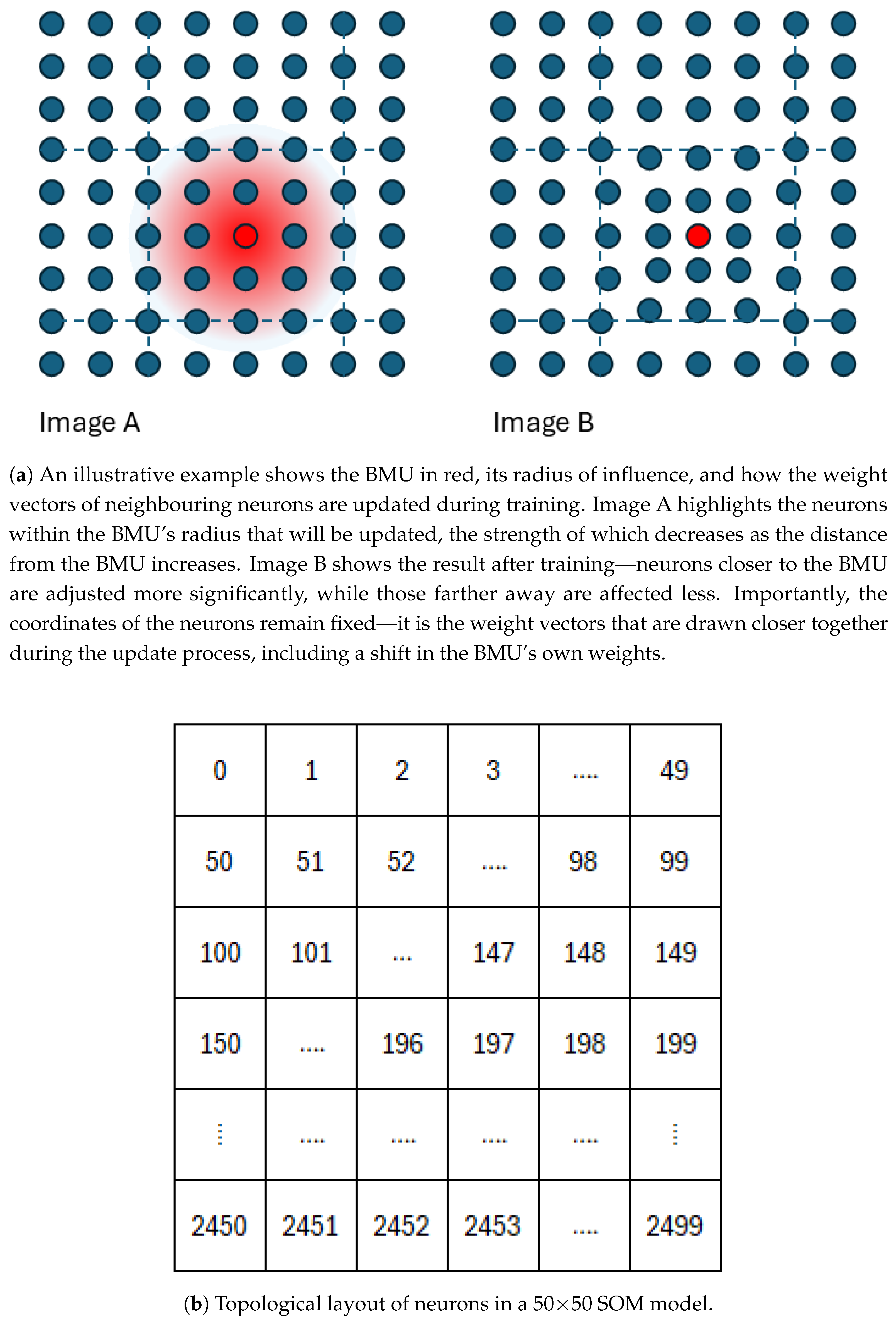
Table 1.
SOM Model execution time (hours and minutes) by number of Neurons.
| Number of Neurons | Execution time (hours and minutes) |
|---|---|
| 225 | 00:38 |
| 400 | 01:28 |
| 625 | 01:54 |
| 900 | 02:31 |
| 1225 | 03:25 |
| 1600 | 09:47 |
| 2025 | 07:17 |
| 2500 | 07:03 |
Table 2.
Comparison of normalised mean weighted distance (MWD) and its gradient for SOM series #1 across different neuron counts.
Table 2.
Comparison of normalised mean weighted distance (MWD) and its gradient for SOM series #1 across different neuron counts.
| Neurons | MWD | Norm. MWD | Gradient |
|---|---|---|---|
| 225 | 0.3269 | 1.453E−03 | E−06 |
| 400 | 0.3150 | 7.874E−04 | E−06 |
| 625 | 0.2916 | 4.665E−04 | E−06 |
| 900 | 0.2719 | 3.021E−04 | E−07 |
| 1225 | 0.2566 | 2.095E−04 | E−07 |
| 1600 | 0.2480 | 1.550E−04 | E−07 |
| 2025 | 0.2356 | 1.163E−04 | E−08 |
| 2500 | 0.2017 | 8.069E−05 | E−08 |
Table 3.
Comparison of normalised mean weighted distance (MWD) and its gradient for SOM series #2 across different neuron counts.
Table 3.
Comparison of normalised mean weighted distance (MWD) and its gradient for SOM series #2 across different neuron counts.
| Neurons | MWD | Norm. MWD | Gradient |
|---|---|---|---|
| 225 | 0.3074 | 1.366E−03 | E−06 |
| 400 | 0.2971 | 7.427E−04 | E−06 |
| 625 | 0.2763 | 4.421E−04 | E−07 |
| 900 | 0.2653 | 2.947E−04 | E−07 |
| 1225 | 0.2511 | 2.050E−04 | E−07 |
| 1600 | 0.2442 | 1.527E−04 | E−07 |
| 2025 | 0.2253 | 1.112E−04 | E−08 |
| 2500 | 0.2298 | 9.192E−05 | E−08 |
Disclaimer/Publisher’s Note: The statements, opinions and data contained in all publications are solely those of the individual author(s) and contributor(s) and not of MDPI and/or the editor(s). MDPI and/or the editor(s) disclaim responsibility for any injury to people or property resulting from any ideas, methods, instructions or products referred to in the content. |
© 2025 by the authors. Licensee MDPI, Basel, Switzerland. This article is an open access article distributed under the terms and conditions of the Creative Commons Attribution (CC BY) license (http://creativecommons.org/licenses/by/4.0/).
Copyright: This open access article is published under a Creative Commons CC BY 4.0 license, which permit the free download, distribution, and reuse, provided that the author and preprint are cited in any reuse.


