Submitted:
22 July 2025
Posted:
23 July 2025
You are already at the latest version
Abstract
In many environmental applications, high quality in-situ measurements are too sparse to resolve the fine scale patterns needed for process understanding and management. We investigated a Bayesian Kriging framework to densify two different coastal data sets: (i) Sea Surface Temperature (SST) in the Algarve region (Portugal), where poin scale measurements (~10km spacing) were densified to a 300m grid and (ii) chlorophyll concentration in the La Spezia embayment (Italy), where satellite and in-situ based 500m measurements were refined to 30m. The model treats the variogram parameters as random variables with weakly informative priors, which are updated by MCMC sampling to yield joint posterior distributions. This hierarchical formulation propagates both measurement noise and structural (variogram) uncertainty to the predictions, producing posterior means and credible intervals at every grid node. Cross validation confirmed robust predictive skill in both pilot sites. The Bayesian Kriging model successfully reconstructed fine scale thermal structures in the Algarve, even when neighbouring SST measurements were separated by several kilometres, underscoring the method’s ability to borrow spatial information and maintain consistent local predictions under severe data sparsity. In La Spezia, the same framework accurately resolved chlorophyll gradients (variability of spatial changes) and estuarine features at 30m resolution. Credible intervals naturally widened in areas far from any measurement yet remained sufficiently narrow elsewhere to guide interpretation, illustrating that the hierarchical formulation captures uncertainty without sacrificing practical detail. Overall, the study shows that Bayesian Kriging can generate high resolution, uncertainty maps from heterogeneous and sparse data records, making it a versatile tool for enhancing remote sensing products and supporting coastal monitoring workflows.
Keywords:
Remote Sensing
; Bayesian Kriging
; Spatial Data Densification
; Uncertainty Quantification
; Geostatistics
; Sea Surface Temperature
; Chlorophyll Concentration
1. Introduction
Environmental monitoring often relies on sparse spatial datasets, where high quality in-situ measurements cover only limited locations. As a result, extensive gaps in coverage hinder our ability to fully understand and model environmental phenomena [1]. Such gaps can bias representations of key processes and adversely impact downstream modeling, predictions and decision making. Spatial data densification seeks to overcome these limitations by transforming sparse measurements into continuous, high resolution data fields, thereby providing a more detailed spatial representation of environmental variables important for climate analysis, resource management and hazard assessment. In recent years, the proliferation of satellite remote sensing has partially alleviated data sparsity by offering broad spatial coverage at increasingly fine resolution [2]. Integrating remote sensing with ground measurements is recognized as a promising strategy to fill data gaps and capture complex spatial patterns [3]. However, effectively merging these heterogeneous data sources and quantifying the remaining uncertainties demand robust geostatistical methods. One classical approach to spatial densification is ordinary kriging, a geostatistical technique that exploits spatial autocorrelation (via variograms) to estimate values at unsampled locations [4]. Ordinary kriging has been widely used to densify environmental data (e.g., mapping rainfall, temperature, or soil properties) thanks to its unbiased predictions and minimal assumption of spatial stationarity. Nonetheless, standard kriging methods face significant challenges when measurements are sparse. In particular, ordinary kriging typically relies on a single empirically derived variogram model with fixed parameters (range, sill, nugget) assumed to be known exactly [5]. In practice, these variogram parameters must be estimated from limited data. Treating them as certain can lead to underestimation of prediction uncertainty, yielding overconfident densification results. Therefore, a single “best fit” variogram ignores the uncertainty in its estimation and it is especially problematic in sparse datasets where different variogram realizations could fit the data nearly equally well. There is a clear need for densification approaches that not only provide spatially continuous estimates but also account for parameter uncertainty to avoid false precision.
Bayesian Kriging has emerged as an effective approach to address these shortcomings by integrating Bayesian statistical inference into the kriging framework [6,7]. Instead of fixing the variogram a priori, Bayesian Kriging treats the variogram parameters as random variables with specified prior distributions, which are then updated in light of the observed data (via Bayes’ theorem) to produce posterior distributions. In this way, any uncertainty in range, sill, or nugget is explicitly quantified and propagated into the predictions. The Bayesian approach allows incorporation of prior knowledge (e.g. from past surveys or expert judgment) on spatial correlation structure when available, while defaulting to noninformative or weakly informative priors when such knowledge is limited. By jointly leveraging the observed spatial structure and prior information, Bayesian Kriging yields more robust densification models that acknowledge the inherent uncertainty in parameter estimation. A key advantage is that this framework produces a full posterior predictive distribution for each unsampled location rather than a single point estimate. The result is that along with a densified value, one obtains credible intervals (Bayesian confidence intervals) that reflect uncertainty stemming from both data noise and model (variogram) uncertainty. This capability is particularly important in environmental applications where understanding the confidence in predictions is as important as the predictions themselves. For example, when mapping pollution or climate variables, decision makers need to know the risk of error before acting. By providing a probabilistic quantification of densification results, Bayesian Kriging supports more nuanced and reliable environmental assessments than deterministic methods.
Another advantage of the Bayesian framework is its flexibility to integrate multi source and heterogeneous data, which is highly relevant in remote sensing. While ordinary kriging can be extended (e.g., co-kriging or regression kriging) to include ancillary variables, Bayesian Kriging offers a coherent way to combine different information streams with associated uncertainties. For instance, heterogeneous datasets from satellite sensors and in-situ measurements can be reconciled within a single Bayesian Kriging model, using priors to account for their differing error characteristics. This external knowledge integration is something that Empirical Bayesian Kriging (EBK) also attempts in an automated fashion. EBK iteratively estimates the variogram by drawing on the data itself (a form of data driven informative prior), effectively simulating multiple variogram realizations to capture parameter uncertainty [8]. Studies have shown that EBK often outperforms classical kriging by mitigating the risk of using a single, suboptimal variogram [9]. In fact, EBK has been reported to produce more accurate and reliable densification results in complex environmental datasets by averaging over many semivariogram possibilities [10]. The fully Bayesian Kriging approach generalizes this idea, providing even greater flexibility: unlike EBK’s purely data derived prior, one can incorporate expert knowledge or physical constraints into the prior and perform formal Bayesian updating to obtain the posterior. This means that Bayesian Kriging can directly include information such as known sensor error variances, expected correlation ranges from past studies, or qualitative knowledge about heterogeneity, which EBK cannot explicitly use. Moreover, Bayesian Kriging yields an exact posterior distribution for predictions (via Bayesian inference) rather than the approximate ensemble output of EBK’s simulations, thereby offering a more principled uncertainty quantification. In summary, Bayesian Kriging retains the ease of use benefits of approaches like EBK (no need for a single fixed variogram) while allowing user guided model priors and producing rigorous probabilistic estimates, making it highly adaptable to diverse scenarios.
Beyond geostatistical kriging variants, machine learning based spatial models have also gained traction for spatial data densification. In remote sensing applications, large volumes of satellite derived covariates (e.g., multispectral indices, DEM, climate reanalysis) can be ingested by machine learning (ML) algorithms to predict environmental variables at unobserved locations [11]. Methods such as random forests, support vector machines and neural networks can capture complex nonlinear relationships between the target variable and auxiliary data, often achieving high predictive accuracy in mapping tasks. For example, in forest biomass estimation, ML models have outperformed traditional regression by better exploiting the rich information in multi sensor remote sensing features [12]. However, a common limitation of these purely data driven approaches is that they do not explicitly account for spatial autocorrelation or local geographic variation. Standard ML models tend to treat all training samples as independent and identically distributed, which can ignore the spatial context (e.g., distance decay of similarity) that geostatistical methods incorporate. This can lead to suboptimal predictions when statistical relationships vary over space (spatial nonstationarity) or when predictions are made in regions with sparse training data. Recent advances like geographically weighted or region specific models (e.g., Geographical Random Forest) attempt to introduce locality into ML predictions, but they still lack the probabilistic output that kriging provides [13]. In general, most machine learning densification methods yield a single predicted value without a measure of uncertainty, unless specialized techniques (such as quantile regression forests, Bayesian neural networks, or ensemble methods) are employed [14]. Ensemble approaches have been explored to bridge this gap, by combining multiple models or generating prediction intervals. For instance, quantile regression ensembles have been used to merge satellite and gauge measurements for precipitation, producing spatial prediction intervals that improve over single model estimates [15]. These developments in ML and ensemble learning are promising for probabilistic mapping, but they operate outside the formal geostatistical framework and may require extensive training data and tuning. In contrast, Bayesian Kriging offers a more interpretable and theoretically grounded approach: it builds on the well understood Gaussian process model of spatial variation, while naturally providing uncertainty estimates. Thus, despite the rise of ML, Bayesian geostatistics remains highly relevant, especially in cases where data are limited and one must leverage physical insight or past knowledge to inform densification.
The benefits of Bayesian Kriging have direct implications for remote sensing and earth observation applications. Many remote sensing products themselves involve densification or data fusion steps. For example, generating gap free land surface temperature maps from satellite overpasses [16], downscaling coarse satellite measurements (like SMAP soil moisture or MODIS ocean color) to finer grids [17] or integrating satellite retrievals with sparse ground stations for air quality mapping [18]. By applying Bayesian Kriging in these contexts, researchers can enhance the spatial resolution of satellite derived datasets while rigorously quantifying uncertainty at each pixel. This leads to more reliable remote sensing data products. Case studies have already demonstrated the value of such an approach: for instance, a Bayesian Kriging regression was employed to estimate near surface air temperature across the United States using satellite land surface temperature as input, yielding competitive accuracy compared to machine learning and providing comprehensive uncertainty estimates for the temperature maps [19]. Furthermore, Bayesian hierarchical models have proven effective in generating more accurate and robust air quality maps by fusing satellite derived aerosol properties with sparse ground-based monitoring data, providing crucial spatially-explicit uncertainty estimates [20]. These examples highlight how a Bayesian framework can effectively exploit remote sensing data (with its large coverage) together with ground truth measurements, resulting in enhanced environmental information content and reliable confidence assessments. The ability to integrate multi resolution datasets and carry forward sensor uncertainties makes Bayesian kriging especially suited for advanced data fusion in remote sensing.
Most of the reported applications, however, operate at regional to continental scales typically densifying from tens of kilometres to ≳1 km resolution where the covariance structure can be assumed relatively smooth over large extents. By contrast, fine scale coastal and estuarine settings often demand sub kilometre grids to resolve sharp near shore gradients. To the best of our knowledge, Bayesian kriging has rarely been deployed in such high resolution, large scale scenarios, partly because the limited number of collocated in-situ observations makes prior specification and covariance estimation more challenging. Addressing this gap, our work demonstrates that, with carefully tuned informative priors and adaptive MCMC, Bayesian kriging can deliver reliable sub kilometre densification of Copernicus marine reanalysis products, thereby extending the method’s utility from broad scale EO analytics to the fine scale coastal zones that are most relevant for local management.
More specifically, in this study we present a Bayesian kriging workflow for spatial densification of sparsely sampled environmental variables and for simultaneous, transparent quantification of prediction uncertainty. We aim to demonstrate Bayesian efficiency in densifying heterogeneous coastal datasets by applying the method to two contrasting testbeds: (i) sea-surface temperature (SST) in the Algarve region and (ii) chlorophyll concentrations in the semi enclosed La Spezia embayment. In both cases, the Bayesian formulation exploits informative but flexible priors for the variogram parameters, propagates their posterior uncertainty into the predictive surface and yields high resolution grids.
2. Theoretical Background
We assume that the spatial process can be described by a Gaussian random field. Let Z(s) denote the environmental variable of interest at location s. We model Z(s) as the sum of a deterministic mean component and a zero mean spatial random effect:
where μ(s) is the trend or mean function and ε(s) is a stochastic term capturing spatially correlated deviations. In our implementation, μ(s) was taken to be either a constant intercept or a simple spatial trend (if justified by site specific exploratory analysis), reflecting the large scale variation in Z(s). The residual term ε(s) is modeled as a stationary Gaussian process with covariance function C(h), where h = |sᵢ - sⱼ| is the distance between any two locations sᵢ and sⱼ. We adopt a Matern type variogram structure because it offers adjustable smoothness through the ν parameter encompassing exponential and Gaussian models as special cases and has well documented numerical stability in Bayesian Gaussian process inference [21,22,23], making it a flexible yet robust choice for representing environmental spatial correlation. The covariance between two points sᵢ and sⱼ is given by:
where θ = {σ², τ², φ} are the variogram parameters (partial sill σ², nugget τ² and range parameter φ), Mν(h; φ) is the Matern correlation function with smoothness ν (we treat ν as fixed) and δᵢⱼ is the Kronecker delta (so τ² is added only when i = j, representing the nugget effect, i.e., microscale variance or measurement error). The range parameter φ governs the distance at which spatial correlation becomes negligible (often defined so that C(h) is about 5% of C(0) when h = φ). For example, in the special case ν = 0.5 (exponential covariance), M₀.₅(h; φ) = exp(−h / φ). The sill (total variance) is C(0) = σ² + τ² and the range (practical correlation range) is defined by φ, while the nugget τ² represents the semivariogram value as h approaches 0. This geostatistical specification corresponds to an ordinary kriging model when μ(s) is constant, extended here into a Bayesian hierarchical model by treating θ as unknown random variables rather than fixed values.
We assign prior distributions to all unknown parameters, namely the mean/trend coefficients and the variogram parameters {σ², τ², φ}. For the mean term (e.g., a constant μ or a vector of regression coefficients β in μ(s) = X(s)^T · β), we use a flat or vague prior (e.g., a normal prior with very large variance) reflecting little prior information. For the variance components σ² and τ², we chose conjugate Inverse Gamma (IG) priors. The IG (Inverse Gamma) distribution ensures positivity and allows us to encode prior knowledge about expected variability. In practice, we set the shape and scale hyperparameters (α, β) of these priors such that the prior means correspond to plausible variance values for each site (e.g., based on sample variance or literature) and with moderate uncertainty. For example, if we expect a priori a process variance around 0.30 (in the units of Z), we might choose σ² ~ IG(α = 2.5, β = 0.45) so that the expected value of σ² is approximately 0.30. Similarly, the nugget prior can be tuned (e.g., if one anticipates the nugget to be about 10% of the total variance). The range parameter φ was given a broad prior on a sensible domain, chosen based on the spatial scale of each study area. We employed a uniform prior for φ (chosen to allow correlations up to the order of the study area extent) unless external information suggested a more informative prior. This reflects a non informative stance on the correlation range, while constraining φ to a realistic interval (to prevent extremely short or long ranges that are implausible).
As a comprehensive strategy our priors for θ = {σ², τ², φ} can be written as:
σ² ~ IG(ασ, βσ), τ² ~ IG(ατ, βτ), φ ~ Uniform(αφ, βφ)
with hyperparameters set as discussed above. These choices can easily be adjusted to incorporate expert knowledge, if any; in our case they were designed to be only mildly informative, serving mainly to stabilize estimation in the presence of very sparse data.
Given the model and priors above, we obtain a well defined posterior distribution for all unknown quantities. The likelihood of the observed data Z = {Z(s₁), ..., Z(sₙ)} under the Gaussian process model is multivariate normal. Combining this likelihood with the prior distributions via Bayes’ theorem yields the joint posterior (see appendix A):
where Σ(θ) is the n × n covariance matrix implied by the variogram parameters θ (with entries Σᵢⱼ = C(|sᵢ − sⱼ|; θ)).
Because this posterior does not have a closed form solution, we resort to numerical sampling methods like the Markov Chain Model Carlo (MCMC) to characterize it. From the posterior samples of β and θ, we can further derive the posterior predictive distribution for Z(s₀) at any new location s₀. In essence, rather than outputting a single densified value, Bayesian Kriging yields a distribution for Z(s₀), obtained by integrating over the uncertainty in β and θ. This is expressed as:
p(Z(s₀) | Z) = ∫ p(Z(s₀) | β, θ, Z) · p(β, θ | Z) dβ dθ (4)
In practice, this integration is accomplished by evaluating the kriging predictor for each sampled pair of {β, θ} and accumulating the results. The predictive distribution is Gaussian for any fixed {β, θ} and the Bayesian result is an average of these Gaussians over the posterior draws. Thus, one readily obtains the posterior predictive mean (the Bayesian Kriging estimate) and credible intervals (Bayesian confidence intervals) for every unsampled location, properly reflecting the uncertainty in σ², τ² and φ as well as the intrinsic kriging variance.
3. Case Studies
3.1. Pilot Site Selection
Two coastal pilot sites were selected to demonstrate the spatial densification approach under different spatial and environmental conditions. The first site, in the Algarve region of southern Portugal, represents an open ocean coastal system at the transition between the East Atlantic and the Mediterranean. The second site, in the La Spezia coastal region of northwestern Italy, represents a semi enclosed estuarine influenced system in the Ligurian Sea. These sites were chosen to encompass distinct oceanographic dynamics wind driven circulation affecting SST in the Algarve, versus riverine and coastal mixing processes affecting chlorophyll concentrations in La Spezia, thereby highlighting the method’s applicability to varied scenarios. Below, we describe the environmental setting and data characteristics for each area, including the target variable for densification, data sources, resolution and preprocessing details.
3.2. The Algarve Pilot Site
The Algarve pilot site lies along the southern Iberian coast, where Atlantic and Mediterranean waters converge. This region experiences energetic coastal dynamics with pronounced wind driven effects. In particular, intermittent Levante easterly winds and prevailing northerly winds create significant hydrodynamic variability, including episodic upwelling and horizontal advection events that strongly influence SST patterns. These processes lead to sharp thermal gradients and fine scale SST features making the area scientifically relevant as a testbed for SST data densification. The chosen study area covers approximately 31km × 31km (~960km²) of coastal ocean. Capturing the SST structure in this transitional and dynamic environment is challenging with sparse measurements, underscoring the need for densification methods that can incorporate multiple data sources and account for uncertainty.
To characterize the SST field in the Algarve region, spatial data were compiled for a representative day (8 November 2024) from heterogeneous sources. Three distinct data sources provided SST measurements over the area:
- ▪
- In-situ ship transects: A set of irregularly spaced SST measurements collected along a research vessel’s transect in the study area (shipborne survey). These moving platform measurements sample a continuous path but leave large portions of the domain unobserved.
- ▪
- Fixed buoy station: SST time series measurements from the permanent oceanographic buoy near Faro (approximately 36°54′ N, 7°54′ W). On the target date, this buoy provided a high accuracy point SST reading, anchoring the dataset at a fixed coastal location.
- ▪
- Satellite reanalysis product: Gridded SST from the ODYSSEA reanalysis system, which blends multi sensor satellite data at about 0.10° resolution. Over the ~30km extent, this corresponds to a coarse grid spacing of roughly 10km, yielding only a few grid points covering the region.
These diverse datasets were harmonized and preprocessed to form a unified input for densification. All SST measurements were mapped to a common spatial reference (WGS84) and checked for consistency. The resulting composite SST dataset remained highly sparse on the order of a few measurement points irregularly scattered across the ~960km² area. The coarsest input (ODYSSEA grid) provided a very limited spatial outline of SST structure and the ship and buoy data, while accurate, sampled only narrow tracks or single points. The goal was to densify the sparse SST measurements onto a fine grid of 300m resolution (approx. 0.003°) covering the Algarve study area, thereby enhancing the spatial detail from an initial scale of ~10km. Such densification aims to highlight the fine scale thermal patterns driven by the Algarve’s interaction of water and atmosphere dynamics that would otherwise be missed.
3.3. The La Spezia Pilot Site
The La Spezia site encompasses the Magra River estuary and its surrounding coastal waters along the Ligurian Sea in NW Italy. This area is characterized by complex land sea interactions, where estuarine discharge and coastal ocean processes intersect. The Magra River delivers freshwater and nutrient loads into the coastal zone, creating a buoyant plume that mixes with saline waters. Wind driven circulation and tidal exchanges further influence the dispersion of this plume. These estuarine and coastal mixing processes lead to strong gradients in water parameters, particularly in chlorophyll concentration which is used as a proxy for phytoplankton biomass and coastal eutrophication. Elevated chlorophyll levels often develop near the river mouth due to nutrient enrichment, while offshore waters remain lower in productivity, resulting in sharp spatial contrasts. The study area in La Spezia covers the immediate coastal zone around the river outlet and adjacent sea, spanning on the order of a few tens of square kilometers (roughly 4 - 5 km across). This region’s environmental complexity and relevance to water quality (eutrophication concerns) make it an important case for testing densification of biogeochemical data.
For the La Spezia coastal region, we analyzed chlorophyll data for March, when nutrient inputs carried by rivers lead to intense blooms, and for October, when concentrations are markedly reduced following the summer period. The primary data source was satellite reanalysis (The primary data source was a Copernicus reprocessed (REP) satellite chlorophyll product (~500m resolution). Although CMEMS classifies REP files as reprocessed observation only composites, the retrospective gap filling and sensor harmonisation justify the common shorthand “satellite reanalysis” used here.) products providing chlorophyll concentration at approximately 500m resolution. These gridded dataset offer regional coverage of the Magra estuary plume and nearby coastal waters. However, even at a 500m spacing, the resolution is relatively coarse, resulting in spatial gaps and lacking the detail needed for nearshore water quality assessment. We therefore subsetted and prepared the data for densification on a much finer grid. A target output resolution of 30m was defined for the densification, covering the coastal study area. This corresponds to a substantial upscaling from the initial 500m data improving the grid resolution by roughly a factor of 17 in linear dimension. The choice of 30m output spacing allows coastal features like narrow nutrient plumes or estuarine fronts to be represented with far greater detail. The spatial patterns observed in the densified chlorophyll maps are consistent with known environmental gradients [24,25,26]. The sparsity challenge here is pronounced; the 500m input grid yields at most a few hundred valid data points over the area and many of those are clustered offshore, with fewer points capturing the immediate vicinity of the river mouth. By applying Bayesian kriging, we fill in the missing nearshore chlorophyll values and generate a continuous 30m chlorophyll map that resolves the fine scale variability associated with the Magra estuary’s influence. This densified product is intended to better depict hotspots of chlorophyll (potential algal blooms) and gradients of eutrophication risk along the La Spezia coast, which are statistically sound for coastal zone management and ecological studies.
Generally, in both pilot sites, the initial measurements are limited in resolution and/or coverage (∼10km scale SST data in the Algarve and 500m chlorophyll data in La Spezia with gaps), posing a challenge for traditional mapping. The densification targets (300m SST grid and 30m chlorophyll grid) substantially increase the spatial detail, enabling finer analysis of the Algarve’s thermal structure and La Spezia’s chlorophyll distribution.
3.4. Densification Grid
To perform spatial densification, we defined a target prediction grid for each study site. For the Algarve SST data, a dense grid with 300m spacing was created, covering the region of interest (approximately a 31km × 31km area near the coast). This resolution (300m) is substantially finer than the ~10km scale of the input measurements, thereby revealing much more localized SST variations. For the La Spezia chlorophyll data, we applied densification onto an even finer grid with 30m spacing, returning the posterior mean value from the resulting prediction surface. The 30m grid was designed to resolve near shore gradients and river plume effects and it was aligned with the UTM projection for that area. The reanalysis data derived chlorophyll dataset at ~500m resolution was subset to a focus area around the Magra River estuary; this subset region (several kilometers across) was then overlayed with the 30m grid for Bayesian kriging. In both cases, the grid nodes that fall on land (land pixels) were excluded from prediction, so that densification was performed only in the ocean/water domain. We selected the grid spacing fine enough to capture expected small scale variability (e.g., coastal SST fronts or chlorophyll patches), but not finer than the scale at which the computational cost would become prohibitive. The result of the Bayesian Kriging procedure is a set of gridded outputs (SST or chlorophyll maps) at the chosen resolution, along with uncertainty measures at each grid cell.
4. Model Specification and Implementation
4.1. Bayesian Kriging Formulation
For both pilot sites, Bayesian Kriging was used to densify the sparse measurements onto fine resolution grids, while explicitly modeling spatial uncertainty through a hierarchical Bayesian framework. Figure 2 illustrates the workflow of this approach, from model formulation and variogram estimation to posterior inference and how the data are transformed from the sparse input locations to the continuous output field via the Bayesian Kriging model. In the following, we detail the model specification, grid setup for densification, evaluation strategy and MCMC parameters.
The steps of the methodology and their roles within this sequence are briefly summarized below.
- ▪
- Model Formation and Fundamental Assumptions: The response variable is treated as a realization of a Gaussian random field defined on geographic space. Stationarity of the increments and second order moments is assumed so that spatial dependence can be characterised solely through the semivariogram function.
- ▪
- Modeling the Mean Component: Large scale trends are represented by a deterministic mean μ(s), typically specified as an intercept only term or a linear combination of geographic covariates. Removing this trend isolates the small scale, spatially correlated residuals that kriging is designed to model.
- ▪
- Covariance Structure and Semivariogram: Spatial autocorrelation is introduced through the Matern covariance function, parameterised by partial sill, range and nugget. The empirical semivariogram provides the initial diagnostic for selecting the functional form and for setting hyperparameters.
- ▪
- Prior Specification: Weakly to non informative priors are assigned to the variogram parameters (e.g. suitable inverse gamma for variances, uniform or log normal for the range) and to the regression coefficients. Knowledge such as expected correlation lengths or measurement error magnitude, is encoded at this stage.
- ▪
- Likelihood Function: Given the assumed Gaussian process, the joint likelihood of the observations is multivariate normal with mean μ(s) and covariance Σ(θ). This term links the data to the unknown parameter vector θ = {σ², τ², ϕ}.
- ▪
- Bayesian Update: Bayes’ rule combines the likelihood with the priors to obtain the posterior distribution p(θ | Z). This update formally propagates both sampling noise and prior uncertainty into all subsequent predictions.
- ▪
- Posterior Predictive Distribution: For any unsampled location s₀, the predictive distribution p(Z(s₀) | Z) is obtained by integrating the kriging conditional mean and variance over the posterior of θ. The result is a full probabilistic surface rather than a single point estimate.
- ▪
- MCMC Sampling: Because the posterior is analytically intractable, MCMC (Gibbs/Metropolis Hastings algorithm) is used to draw a representative ensemble of θ values. Convergence diagnostics (trace plots, Geweke z-scores, acceptance rates) ensure adequate exploration of the space parameter.
- ▪
- Evaluation of Predictive Performance: Posterior draws are summarised to compute point predictions, 95% credible intervals and uncertainty maps. Accuracy is quantified with cross validation metrics RMSE, MAE, R², while coverage tests verify that the empirical proportion of observations falling inside the credible bands matches the nominal level.
- ▪
- Model Validation: Residual analyses assess whether assumptions are met and whether additional covariates or alternative priors are required. Validated models are then carried forward to generate the final, high resolution densified grids.
4.2. MCMC Configuration
Posterior inference was carried out using Markov Chain Monte Carlo simulation. We implemented a Gibbs sampler with conjugate updates for the variance components and Metropolis - Hastings steps for any parameters without closed form full conditionals. In particular, at each MCMC iteration the algorithm samples sequentially from: (1) the conditional posterior of the mean parameters β (a multivariate normal, or in the scalar case of a constant mean, a univariate normal), (2) the conditional posterior of the partial sill σ² (IG, given the Gaussian likelihood and IG prior), (3) the nugget τ² (IG distribution) and (4) the range φ (for which we used a random walk Metropolis step, since φ’s conditional distribution is not standard). By iterating these draws, the chain of {β, σ², τ², φ} values converge to samples from the joint posterior in Equation (3). We ran the sampler for a sufficiently large number of iterations to ensure convergence and robust estimation of posterior quantities. In practice, each site’s model was run with multiple chains and over approximately 200.000 iterations and thinning every 10 iterations to reduce autocorrelation, discarding an initial burn-in portion. Convergence was diagnosed by inspecting trace plots of the parameters and using the Gelman - Rubin statistic Rhat, confirming that all Rhat ≈ 1.0 and that each parameter’s sample trace had mixed well. The posterior samples were then used to compute summary statistics: for example, the posterior mean and 95% credible interval for each variogram parameter (providing a Bayesian estimate of range, sill and nugget for the site) and the predictive posterior mean and intervals for each grid cell in the densified output map. While Bayesian Kriging is more computationally intensive than ordinary kriging due to the need to sample across a high dimensional parameter space the chosen MCMC approach proved tractable for our problem sizes. We emphasize that careful tuning of the sampler (e.g., step sizes for the Metropolis updates) was performed to balance acceptance rates and convergence speed. After obtaining the final sample pools, we verified that the posterior predictive distributions were coherent: for instance, the width of credible intervals widened appropriately in regions far from any measurements (reflecting greater uncertainty) and narrowed near the sampled locations, demonstrating that the MCMC based inference correctly propagated the variogram uncertainty into the spatial predictions.
4.3. Computational Setup
All computations were carried out in the R statistical computing environment utilizing a combination of base R and geostatistical packages (libraries). The core Bayesian Kriging models were implemented using custom code, the spBayes and geoR packages [27,28,29], which provide tools for spatial regression, covariance modeling and MCMC sampling.
Pilot runs (simulations) were initially conducted on subsets of each dataset to calibrate hyperparameters and explore model sensitivity to priors. Once suitable priors and proposal distributions were selected, the full posterior inference was performed over the entire spatial domain. Computations were performed on a server equipped with an Intel Core i7 CPU and 64 GB of RAM; runtime ranged from ~85 min for La Spezia to ~135 min for Algarve, depending mainly on the number of measurements, the prediction grid density and the number and length of the MCMC chains needed for convergence. Classical MCMC algorithms require O(n3) operations to iterate the correlation matrix decompositions.As the dimensions of the study area increased, the calculation time increased almost geometrically. Posterior predictive maps were generated by applying Bayesian Kriging formulas at each target grid cell, using posterior draws of variogram parameters. Summary maps (posterior mean, 95% credible intervals) were created using the raster, terra and ggplot2 packages.
This computational framework allowed for efficient, transparent and reproducible Bayesian Kriging workflows in both case studies, with full uncertainty quantification and diagnostic tools to support scientific densification.
5. Results and Evaluation
We evaluated the performance of the Bayesian Kriging densification through metrics and diagnostics. The Markov Chain Monte Carlo sampling showed good mixing and convergence in both regions. Key diagnostics include:
- ▪
- Acceptance rates: ~0.35 for key parameters indicating efficient proposal acceptance.
- ▪
- Convergence tests: Gelman - Rubin potential scale reduction factors were ≈1.00 for all monitored parameters and Geweke’s z-scores (two sided test) were not significant (p > 0.05), indicating no evidence of non convergence.
- ▪
- Trace plots: Representative chains stabilized relatively quickly after burn-in with no apparent trends. The multiple experiments (poilot runs) we did showed that quick convergence depends directly on the size of the study area.
- ▪
- Cross validation performance assessment using RMSE, MAE and R² metrics.
5.1. Algarve, SST Densification
Initial tests (pilot runs) were performed on subsets of the data and the acceptance rates, trace plots (behavior of MCMC chains) and diagnostic indicators (Geweke criterion) were checked to decide on the values of the hyperparameters. After satisfactory settings (priors, MCMC samples) are found, the model is run on the entire dataset to produce estimates (kriged predictions) on a 300m grid. The main challenge arises from the large computational burden, especially when the number of points (observations) is large.
The final Bayesian estimation of SST on a 300m × 300m grid yielded satisfactory predictions, as shown by the evaluation metrics. This suggests that the spatial model used captured the variability and spatial correlation of SST satisfactorily and validly. Furthermore, the visual comparison of the initial measurements with the predicted values (Figure 3, bottom right) showed that the majority of the points fit well, with small deviations mainly reflected at local boundaries or in areas with minimal initial measurements. The calculated uncertainty (Table1) was depicted on graphs where the color and size of the points reflect the level of variation or residuals (Figure 3, bottom left).
Cross validation and error metrics indicate high performance for Algarve. Comparing the kriged estimates to the initial SST measurements (at their locations) yields a very low RMSE (0.015 °C) and MAE (0.0067 °C) with a near unity R²(0.99) and 95% prediction interval ≈ ±0.045 °C. The model explains almost all of the observed variance in SST. Bayesian Kriging captured the spatial structure of the SST field remarkably well. Only small deviations were observed between predictions and measurements. A visual comparison (Figure 3, bottom right) showed that almost all measurement points align closely with the predicted values; the deviations were small, occurring mainly at a few local boundary areas. This suggests there was no significant systematic bias. The residuals (measurement minus prediction) appeared randomly distributed, confirming the model did not consistently over or under predict in any region.
The algorithm also provided uncertainty estimates for the SST predictions, which were reassuringly low. The posterior predictive standard deviation for SST was usually in the order of a few decimal places. For instance, the median predicted standard deviation was ~0.09°C (Table 1) and the mean was ~0.10°C. Even the maximum standard deviation in the domain (generally at the far edges or in data poor spots) was only 0.22°C. This corresponds to a 95% credible interval of roughly ±0.44°C in the most uncertain location and for most locations the 95% intervals were much tighter (± 0.18 - 0.20°C around the median uncertainty). Figure 4 further highlights that the histogram of average SST values reveals that most adjusted temperatures are close to 20°C; the histogram of predicted variance shows that almost all values are clustered around σ² ≈ 0.012 to 0.014 (i.e. σ ≈ 0.11 - 0.12°C) which reflects the low residual uncertainty; warmer temperatures (e.g. 20.5–21°C) contribute more to the total variance. The vast majority of grid cells have very low prediction variance. Notably, the typical prediction uncertainty (σ ≈ 0.10°C) is substantially smaller than the natural spatial variability of SST in the region. When SST predictions were binned by temperature zones, the internal SST variability within each zone was around 0.45°C [sqr(20oC)], which far exceeds the model’s residual uncertainty. This indicates that the model’s uncertainty is very small, the kriging predictions are confident relative to the actual environmental variability. Such low uncertainty, even after a 33 fold (10.000/300) increase in resolution, attests to the reliability of the Bayesian Kriging results for Algarve. It is worth noting that this case required careful variogram modeling due to the sparse data so that the final result would be a high-resolution SST product with very high accuracy and repeatability.
5.2. La Spezia (Italy), Chlorophyll Densification
The data were processed to extract values in a 30m (Figure 5 and Figure 6right) grid that corresponds to roughly a 17x increase in the initial spatial resolution. In Figure 7 we see the behavior of MCMC chains for the Bayesian Kriging parameters for the March and September 2024 data
Investigating chlorophyll levels in March in this coastal area is of great interest, as the seasonal increase in freshwater discharge from the Magra River is likely to introduce elevated amounts of nutrients into the marine environment. This nutrient influx can stimulate phytoplankton growth, potentially leading to significantly higher chlorophyll concentrations compared to other months (Figure 8 and Figure 10). By analyzing March data alongside September measurements (Figure 8, Figure 9 and Figure 10), researchers can better understand the seasonal dynamics of coastal productivity, assess the impact of terrestrial nutrient inputs and evaluate the implications of climate variability on marine ecosystems. During the summer months and early autumn, the river runoff decreases due to reduced rainfall and lower flow, which limits the input of nutrients to the coastal environment. As a result, lower chlorophyll concentrations are expected compared to the March period, when the increased river flow enhances the nutrient load and favors the growth of phytoplankton.
The application of Bayesian kriging for spatial densification of chlorophyll concentrations in the coastal area of La Spezia demonstrated very high predictive performance and robustness. The model achieved very low prediction errors (RMSE = 0.026 mg·m⁻³, MAE = 0.011 mg·m⁻³) and an excellent coefficient of determination (R² = 0.99), indicating that it captured nearly all the variability in the observed data. The residual analysis confirmed the absence of systematic bias and revealed spatially balanced errors across the study area. Furthermore, the model's 95% uncertainty interval (±0.052 mg·m⁻³) remained within ecologically acceptable limits, underscoring the reliability of the densified chlorophyll fields.
Compared to the Algarve case, the La Spezia densification was more straightforward due to the denser initial sampling and smaller upscaling factor and the performance metrics reflect this ease. The success in La Spezia further underscores the robustness of the Bayesian Kriging approach for spatial data densification in coastal environments. The model effectively captured fine scale chlorophyll structures such as coastal nutrient gradients, while also quantifying the low uncertainty, making the resulting high resolution data highly reliable for remote sensing and ecological applications.
6. Discussion - Conclusions
6.1. Comparative Performance in Algarve vs. La Spezia
Kriging approach yielded consistently high accuracy in both pilot sites, albeit under different environmental conditions. In the Algarve (southern Portugal), a dynamic Atlantic - Mediterranean transition zone characterized by Levante wind driven SST variability, our model successfully densified (after too many pilot runs, testing different prior distributions and checking their hyper parameters) coarse SST data (~10km resolution) to a fine 300m grid. This produced exceptionally low densification errors (e.g., RMSE ≈ 0.015°C) and a near perfect coefficient of determination (R² ≈ 0.99). The predicted SST field captured fine scale thermal patterns near the Strait of Gibraltar. Similarly, in La Spezia (northwestern Italy), a coastal estuarine environment with complex land sea interactions and strong chlorophyll gradients from riverine input, Bayesian Kriging proved equally effective. Starting from a ~500m reanalysis satellite derived chlorophyll map, the model generated a 30m resolution chlorophyll field with very low error (RMSE = 0.026 mg·m⁻³) and R² = 0.99. The densified chlorophyll maps accurately reproduced the spatial pattern of decreasing concentrations with distance offshore, reflecting nutrient dilution from the Magra River outflow. Notably, no significant bias was detected in either case and residuals were spatially balanced, indicating that the model did not consistently over or under predict in any region. The uncertainty bounds provided by the Bayesian Kriging (e.g., a 95% credible interval of ±0.052 mg·m⁻³ in La Spezia) were tight and encompassed nearly all observed errors, giving confidence that the densified outputs are both accurate and reliable. These parallel outcomes in two distinct coastal settings confirm that the Bayesian Kriging framework is robust across different variables and scales, from SST in open ocean influenced waters to chlorophyll in a eutrophic coastal bay.
6.2. Implications for Hypotheses and Broader Context
These findings strongly support our working hypothesis that a fully Bayesian treatment of spatial densification enhances both accuracy and uncertainty characterization relative to classical methods. By treating variogram parameters as uncertain and integrating prior knowledge, even if weakly informative, Bayesian Kriging was able to address limitations of ordinary kriging, which traditionally relies on a single fixed variogram estimate. The performance (R² ~0.99) in both study areas suggests that explicitly modeling the uncertainty in spatial correlation prevents underfitting due to variogram misspecification, thereby capturing virtually all the measurable spatial variability. This outcome aligns with broader trends in environmental remote sensing and spatial statistics that emphasize data fusion and uncertainty quantification. Recent studies [30,31,32,33] have shown that Bayesian spatial frameworks can effectively combine sparse in-situ measurements with broad coverage remote sensing data, yielding enriched information content and dependable confidence intervals. Our results contribute to this narrative by demonstrating in real world cases that Bayesian Kriging produces high resolution maps with quantifiable credibility. In practical terms, this means environmental managers can obtain densified SST or chlorophyll maps that are not only precise but also come with rigorous estimates of uncertainty, an important consideration for decision making under risk. Furthermore, the success of Bayesian Kriging in two different coastal regimes indicates its generality; the method can adapt to varying spatial structures (from relatively smooth SST fields to more heterogeneous chlorophyll distributions) without loss of performance. This adaptability is especially pertinent given the growing availability of multi source datasets in remote sensing. Compared to machine learning approaches often used for downscaling, the Bayesian Kriging method achieved competitive accuracy with the added benefit of physics informed transparency and uncertainty bounds, as evidenced in our study and others. Overall, our discussion underscores that accounting for geostatistical parameter uncertainty is not just a theoretical exercise, but one that yields tangible improvements in environmental data densification, corroborating earlier calls in the literature for Bayesian methods In geospatial analysis.
6.3. Influence of Prior Specification on Densification Quality
A key finding from this work is the strong influence of prior specification on the accuracy and realism of Bayesian Kriging outputs. In a Bayesian framework, the choice of prior distributions for variogram parameters (nugget, sill, range, etc.) effectively injects assumptions into the model. Our implementation leveraged this by using reasonably broad priors, for example, appropriate IG distributions for variance components and a constrained uniform range based on empirical semivariogram analysis, to reflect variability while avoiding overconfidence. This careful prior tuning was instrumental in stabilizing the densification. In practice, we observed that if priors were set too loosely (vague), the MCMC sampling occasionally explored extreme variogram values, leading to either over smoothed fields or unrealistically noisy predictions. Conversely, overly tight priors could bias the results, underestimating natural variability. By grounding the priors on literature references and performing many pilot runs, we ensured that the posterior variogram realizations remained physically sensible. This not only improved predictive performance but also yielded credible densification uncertainty. In essence, the priors act as a form of regularization, especially critical when the sample data are limited or unevenly distributed. Our findings echo earlier studies [34,35] that showed incorporating expert knowledge or empirical evidence into the variogram priors leads to more realistic spatial predictions and narrower uncertainty bands. It is important to note that the use of Bayesian Kriging requires careful attention to prior selection; it is a sensitive knob that can markedly affect densification outcomes.
6.4. Limitations and Future Research Directions
The present work is confined to two temperate water test sites and relies on relatively short time slices, so the conclusions may not generalise to tropical latitude systems or to strongly non stationary seasons. Although the prior specifications were informed by empirical variograms derived from the data, the selection of hyperparameters for the prior distributions did not follow a rigid, systematic protocol. Instead, they were tailored on a case basis, through subjective choices, manual adjustments, and iterative tuning, to better align with the specific characteristics of the dataset and research objectives.
Further improvements can be made to strengthen Bayesian Kriging for environmental mapping. First, systematic prior specification e.g., penalised complexity priors that adapt to regional data, would reduce ad hoc tuning and improve robustness. Second, scalable inference across geographically extensive or high resolution study areas will likely require adaptive, data driven knot selection schemes that optimize both the number and placement of knots, balancing the O(n³) computational cost with predictive accuracy. Finally, extending the framework to fully spatiotemporal models, where Bayesian updating is performed sequentially as new observations arrive, would enable real time densification and forecasting with propagated uncertainty.
Author Contributions
Conceptualization, V.A, V.K.; methodology, V.A., V.K.; software, V.A.; validation, V.A; formal analysis, V.A., V.K.; investigation, V.A.; resources, V.A., V.K.; data curation, V.A., V.K.; writing-original draft preparation, V.A.; writing-review and editing, V.K., V.A; visualization, V.A.; supervision, V.K.; project administration, V.K.; funding acquisition, V.K.
Funding
The present research study has been financially supported by the project “THETIDA”, funded by European Union’s Horizon Europe Research and Innovation program HORIZON-CL2-2022-HERITAGE-01 under grant agreement N. 101095253.
Data Availability Statement
The original contributions presented in the study are included in the article. Further inquiries can be directed to the corresponding author.
Acknowledgments
The authors wish to the thank the funding body for financially supporting the implementation of the present work and also the reviewers for their constructive feedback that helped improving the initially submitted manuscript.
Conflicts of Interest
The authors declare no conflicts of interest.
Abbreviations
The following abbreviations are used in this manuscript:
| SST | Sea Surface Temperature |
| EBK | Empirical Bayesian Kriging |
| MCMC | Markov Chain Monte Carlo |
| RMSE | Root Mean Square Error |
| MAE | Mean Absolute Error |
| R² | Coefficient of Determination |
| LOOCV | Leave One Out Cross Validation |
| UTM | Universal Transverse Mercator (projection) |
| IG | Inverse Gamma (distribution) |
Appendix A
Appendix A.1
Joint Posterior Derivation for Bayesian GP Regression (Spatial Kriging)
Model Specification
Consider observed data Z(s)∈R at spatial locations s1,…,sn. Let Z=[Z(s1),…,Z(sn)]T be the n-vector of responses. We assume a spatial linear regression model with a Gaussian process (GP) residual:
Z(s) = X(s)β + ϵ(s)
where X(s) is a 1×p row-vector of covariates (with known design matrix X∈Rn×p stacking X(si) for i=1,…,n ) and β is a p-dimensional vector of regression coefficients. The residual term ϵ(s) is modeled as a zero-mean Gaussian process with covariance parameters θ={σ2,τ2,ϕ}. In particular, ϵ(⋅) has covariance function Σ(θ) so that:
Here, ρ(dij∣ϕ) is a correlation function (depending on distance dij=∣si - sj∣ and range parameter ϕ) and τ2 represents the nugget (micro-scale variance or measurement error). For example, one common choice is an exponential covariance where:
so:
Given β and θ, the data vector Z follows a multivariate normal distribution:
In other words, conditional on parameters (β,σ2,τ2,ϕ), we have:
where R(ϕ) is the n×n spatial correlation matrix with (i,j) entry ρ(dij∣ϕ).
Likelihood Function
Under the model above, the likelihood (sampling density) for the observed data Z given parameters (β,θ) is the multivariate Gaussian density with mean Xβ and covariance Σ(θ). Writing Σ=Σ(θ) for notation brevity, the likelihood is:
This is the standard form of a multivariate normal (Gaussian) density. Here ∣Σ∣ denotes the determinant of the n×n covariance matrix Σ(θ), which depends on σ2, τ2 and ϕ. The quadratic form (Z−Xβ)T Σ-1 (Z−Xβ) is the Mahalanobis distance measuring how far the data are from the mean Xβ in units of the covariance Σ.
Prior Distributions
To complete the Bayesian model, we specify prior distributions for all parameters (β,σ2,τ2,ϕ). We assume the priors factorize (independent a priori):
Regression coefficients (β):We assign a flat (uninformative) prior to β, meaning p(β) ∝1 (a constant) over Rp. (In practice, one may use a very vague Gaussian prior for β, e.g., β ∼ N(0,Σβ) with Σβ large, which approaches a flat prior as Σβ → ∞) This reflects no strong prior information on the mean trend.
Process variance (σ2):We assume σ2 has an Inverse Gamma (IG) prior: σ2∼IG(ασ,βσ). Here ασ is the shape parameter and βσ the scale parameter of the IG. In density form, this prior means:
for σ2 > 0. IG is a convenient choice for a variance parameter as it ensures σ2 > 0 and is conjugate to the normal likelihood in simpler settings. Typical hyperparameter values are chosen to be small (e.g., ασ = 2, βσ = 1) to make the prior vague.
Nugget variance (τ2):Similarly, we assign τ2 ∼ IG(ατ,βτ) independently. This implies:
for τ2 > 0. Again, vague choices for shape and scale (e.g., ατ = 2, βτ =1) are common.
Range/decay parameter (ϕ):We assume a uniform prior for ϕ over some interval [a,b] that covers the plausible range of spatial correlation. For example, ϕ∼U(a,b) might be taken so that [a,b] spans from very short-range to very long-range dependence given the spatial domain. In density form:
i.e., constant on [a,b] (and zero outside). This reflects a non-informative prior belief about the range parameter (sometimes a weakly informative prior like a broad Gamma distribution is used, but we will use Uniform as stated).
To summarize, our prior specifications (assumed independent) are:
In particular:
p(β) ∝ 1,
,
,
p(ϕ) ∝ 1on [a,b].
These choices are used in the Bayesian spatial model.
Joint Posterior Derivation
Given the likelihood and prior above, we can derive the joint posterior distribution for the parameters (β,σ2,τ2,ϕ) by applying Bayes’ theorem. Bayes’ rule in this context is:
Here p(Z) is the marginal likelihood (evidence), a normalizing constant independent of the parameters. In practice, we usually work with the unnormalized posterior (often called the posterior kernel), since p(Z) is intractable to compute analytically. Thus, up to a constant of proportionality, the joint posterior density is given by the product of the likelihood and all prior densities:
Now we substitute the expressions for the likelihood and priors derived above. Using the Gaussian likelihood and the independent priors, we get:
Each factor above corresponds to:
the likelihood of Z,
the flat prior on β (which contributes a constant),
the prior on σ2,
the prior on τ2,
the prior on ϕ.
Because we are using a proportionality (∝), we have omitted constant normalization factors that do not depend on the parameters. The indicator 1[a,b](ϕ) simply enforces that ϕ lies in its prior support [a,b].
We can simplify this posterior kernel by dropping any remaining constant terms. Noting that (2π)-n/2 and (b-a)-1 are constants, the joint posterior density (up to normalization) can be written compactly as:
for ϕ∈[a,b] and σ2,τ2 > 0. This expression is the joint posterior p(β,θ∣Z), where θ = {σ², τ², ϕ}. It combines the information from the data (through the likelihood) with the prior beliefs. In an actual analysis, one could plug in the specific forms of Σ(θ) (e.g., Σ(θ) = σ2R(ϕ) + τ2I) to make this more explicit. The posterior is generally not of a standard form that can be sampled or summarized analytically, due to the coupling of β and Σ(θ) and the non conjugacy of ϕ in the covariance. However, this is the complete expression that defines our posterior knowledge of the parameters after observing Z.
(For completeness, one could factor this joint posterior further into conditional distributions. For instance, if β had a conjugate Gaussian prior, the conditional posterior p(β∣σ2,τ2,ϕ,Z) would be multivariate normal (a generalized least squares update) and p(σ2,τ2,ϕ∣Z) would be the marginal posterior of the covariance hyperparameters. However, here we present the full joint form without integrating out any parameters.)
Posterior Inference via MCMC
The derived joint posterior p(β,σ2,τ2,ϕ|Z) above typically cannot be normalized or sampled from directly in closed form. In practice, Markov Chain Monte Carlo (MCMC) methods are used to perform posterior inference. The posterior expression allows us to evaluate the density (up to a constant) for any candidate parameter values, which is exactly what algorithms like Gibbs sampling and Metropolis-Hastings require. For example, one can construct a Gibbs sampler that iteratively draws each parameter (or block of parameters) from its full conditional distribution derived from the joint posterior. In our model, given the other parameters:
The conditional distribution p(β|σ2,τ2,ϕ,Z) is (for a flat prior) proportional to a Gaussian likelihood, which yields a multivariate normal distribution (the posterior of β given θ is the generalized least-squares estimator with covariance (XTΣ(θ)-1X)-1). If a vague Normal prior on β were used instead of flat, this update remains conjugate Gaussian.
The conditional p(σ2|β,τ2,ϕ,Z) (with β,ϕ,τ2 fixed) can be shown to follow an IG distribution, since the likelihood contributes a sum of squares term in Z-Xβ that, combined with the σ2 prior, yields an IG posterior (this is a consequence of conjugacy for variance in a normal model). Likewise, p(τ2|β,σ2,ϕ,Z) is IG by a similar reasoning on the nugget residuals.
The conditional p(ϕ|β,σ2,τ2,Z) is not of standard form (the correlation parameter ϕ enters ∣Σ∣∣Σ∣ and Σ-1 in a non-linear way). Thus, one would update ϕ using a Metropolis - Hastings step: propose a new ϕ∗ and accept/reject it based on the ratio of the posterior kernels. Alternatively, advanced samplers like slice sampling or adaptive Metropolis can be used.
By cycling through these updates, the Gibbs sampler produces a Markov chain whose stationary distribution is the joint posterior p(β,σ2,τ2,ϕ|Z). After a sufficient burn-in period, one can collect samples to approximate posterior expectations and credible intervals for all parameters. In summary, the closed-form expression of the posterior derived above is fundamental for implementing MCMC: it provides the functional form needed to draw posterior samples of (β,θ) and thereby perform full Bayesian inference for the spatial regression model.
References
- Wang, R.; Pan, D.; Guo, X.; Sun, K.; Clarisse, L.; Van Damme, M.; Coheur, P.-F.; Clerbaux, C.; Puchalski, M.; Zondlo, M.A. Bridging the spatial gaps of the Ammonia Monitoring Network using satellite ammonia measurements. Atmospheric Meas. Tech. 2023, 23, 13217–13234. [Google Scholar] [CrossRef] [PubMed]
- Tian, Y.; Duan, M.; Cui, X.; Zhao, Q.; Tian, S.; Lin, Y.; Wang, W. Advancing application of satellite remote sensing technologies for linking atmospheric and built environment to health. Front. Public Heal. 2023, 11, 1270033. [Google Scholar] [CrossRef] [PubMed]
- Zhang, J.; Li, X.; Yang, R.; Liu, Q.; Zhao, L.; Dou, B. An Extended Kriging Method to Interpolate Near-Surface Soil Moisture Data Measured by Wireless Sensor Networks. Sensors 2017, 17, 1390. [Google Scholar] [CrossRef] [PubMed]
- Li, J.; Heap, A.D. A review of comparative studies of spatial interpolation methods in environmental sciences: Performance and impact factors. Ecol. Informatics 2011, 6, 228–241. [Google Scholar] [CrossRef]
- Le, N.D.; Zidek, J.V. Interpolation with uncertain spatial covariances: A Bayesian alternative to Kriging. J. Multivar. Anal. 1992, 43, 351–374. [Google Scholar] [CrossRef]
- Omre, H. Bayesian kriging?Merging observations and qualified guesses in kriging. J. Int. Assoc. Math. Geol. 1987, 19, 25–39. [Google Scholar] [CrossRef]
- Handcock, M.S.; Stein, M.L. A Bayesian Analysis of Kriging. Technometrics 1993, 35, 403–410. [Google Scholar] [CrossRef]
- Krivoruchko, K.; Gribov, A. Evaluation of empirical Bayesian kriging. Spat. Stat. 2019, 32, 100368. [Google Scholar] [CrossRef]
- Veronesi, F.; Schillaci, C. Comparison between geostatistical and machine learning models as predictors of topsoil organic carbon with a focus on local uncertainty estimation. Ecol. Indic. 2019, 101, 1032–1044. [Google Scholar] [CrossRef]
- Mishra, U.; Gautam, S.; Riley, W.J.; Hoffman, F.M. Ensemble Machine Learning Approach Improves Predicted Spatial Variation of Surface Soil Organic Carbon Stocks in Data-Limited Northern Circumpolar Region. Front. Big Data 2020, 3. [Google Scholar] [CrossRef] [PubMed]
- Cui, T.; Li, X.; Zhang, L.; Du, J.; Wang, Z. ; A Bayesian Approach to Estimate the Spatial Distribution of Seawater Temperature Using Remote Sensing Data. Remote Sens. 2021, 13, 1234. [Google Scholar] [CrossRef]
- Zaresefat, M.; Derakhshani, R.; Griffioen, J. Empirical Bayesian Kriging, a Robust Method for Spatial Data Interpolation of a Large Groundwater Quality Dataset from the Western Netherlands. Water 2024, 16, 2581. [Google Scholar] [CrossRef]
- Takoutsing, B.; Heuvelink G., B.M. Comparing the prediction performance, uncertainty quantification and extrapolation potential of regression kriging and random forest while accounting for soil measurement errors. Geoderma 2022, 428, 116192. [Google Scholar] [CrossRef]
- Bykov, K.; Höhne, M.-C.; Creosteanu, A.; Müller K., R.; Klauschen, F.; Nakajima, S.; Kloft, M. ; Explaining Bayesian Neural Networks; arXiv:2108. 1 0346. [CrossRef]
- Vicedo-Cabrera, A.M.; Biggeri, A.; Grisotto, L.; Barbone, F.; Catelan, D. A Bayesian kriging model for estimating residential exposure to air pollution of children living in a high-risk area in Italy. Geospat. Heal. 2013, 8, 87–95. [Google Scholar] [CrossRef] [PubMed]
- Lompar, M.; Lalić, B.; Dekić, L.; Petrić, M. Filling Gaps in Hourly Air Temperature Data Using Debiased ERA5 Data. Atmosphere 2019, 10, 13. [Google Scholar] [CrossRef]
- Senanayake, I.P.; Arachchilage, K.R.L.P.; Yeo, I.-Y.; Khaki, M.; Han, S.-C.; Dahlhaus, P.G. Spatial Downscaling of Satellite-Based Soil Moisture Products Using Machine Learning Techniques: A Review. Remote. Sens. 2024, 16, 2067. [Google Scholar] [CrossRef]
- Hoff, R. M.; Christopher, S. A. Remote sensing of particulate pollution from space: have we reached the promised land? Journal of the Air & Waste Management Association 2009, 59, 645–675. [Google Scholar]
- Agyeman, P.C.; Kebonye, N.M.; John, K.; Borůvka, L.; Vašát, R.; Fajemisim, O. Prediction of nickel concentration in peri-urban and urban soils using hybridized empirical bayesian kriging and support vector machine regression. Sci. Rep. 2022, 12, 1–16. [Google Scholar] [CrossRef] [PubMed]
- Shaddick, G.; Thomas, M.L.; Amini, H.; Broday, D.M.; Cohen, A.; Frostad, J.; Green, A.; Gumy, S.; Liu, Y.; Martin, R.V.; et al. Data Integration for the Assessment of Population Exposure to Ambient Air Pollution for Global Burden of Disease Assessment. Environ. Sci. Technol. 2018, 52, 9069–9078. [Google Scholar] [CrossRef] [PubMed]
- Stein, M.L. Interpolation of Spatial Data: Some Theory for Kriging; Springer: New York, NY, USA, 1999; 87, 103. [Google Scholar] [CrossRef]
- Rasmussen, C.E.; Williams, C.K.I. Gaussian Processes for Machine Learning; MIT Press: Cambridge, MA, USA, 2006; pp. 84–89. ISBN 978-0-262-18253-9. [Google Scholar]
- Lindgren, F.; Rue, H.; Lindström, J. An Explicit Link between Gaussian Fields and Gaussian Markov Random Fields: The Stochastic Partial Differential Equation Approach. J. R. Stat. Soc. Ser. B (Statistical Methodol. 2011, 73, 423–498. [Google Scholar] [CrossRef]
- Poulain, P.-M.; Mauri, E.; Gerin, R.; Chiggiato, J.; Schroeder, K.; Griffa, A.; Borghini, M.; Zambianchi, E.; Falco, P.; Testor, P.; et al. On the dynamics in the southeastern Ligurian Sea in summer 2010. Cont. Shelf Res. 2020, 196, 104083. [Google Scholar] [CrossRef]
- Lapucci, C.; Rella, M.A.; Brandini, C.; Ganzin, N.; Gozzini, B.; Maselli, F.; Massi, L.; Nuccio, C.; Ortolani, A.; Trees, C. Evaluation of empirical and semi-analytical chlorophyll algorithms in the Ligurian and North Tyrrhenian Seas. J. Appl. Remote. Sens. 2012, 6, 063565–1. [Google Scholar] [CrossRef]
- Fernández-Tejedor, M.; Velasco, J.E.; Angelats, E. Accurate Estimation of Chlorophyll-a Concentration in the Coastal Areas of the Ebro Delta (NW Mediterranean) Using Sentinel-2 and Its Application in the Selection of Areas for Mussel Aquaculture. Remote. Sens. 2022, 14, 5235. [Google Scholar] [CrossRef]
- Finley, A.; Banerjee, S. spBayes: Univariate and Multivariate Spatial-Temporal Modeling. R package version 0.4-8; 2024; DOI: 10.32614/CRAN.package.spBayes; https://CRAN.R-project.org/package=spBayes.
- Finley, A.O.; Banerjee, S.; E.GElfand, A. spBayesfor Large Univariate and Multivariate Point-Referenced Spatio-Temporal Data Models. J. Stat. Softw. 2015, 63, 1–28. [Google Scholar] [CrossRef]
- Ribeiro Jr PJ, Diggle P (2025). geoR: Analysis of Geostatistical Data. R package version 1.9-5; DOI:10.32614/CRAN.package.geoR; https://CRAN.R-project.org/package=geoR.
- Shi, Y.; Zhou, X.; Yang, X.; Shi, L.; Ma, S. Merging Satellite Ocean Color Data With Bayesian Maximum Entropy Method. IEEE J. Sel. Top. Appl. Earth Obs. Remote. Sens. 2015, 8, 3294–3304. [Google Scholar] [CrossRef]
- He, S.; Wong, S.W. Spatio-temporal data fusion for the analysis of in situ and remote sensing data using the INLA-SPDE approach. Spat. Stat. 2024, 64, 100863. [Google Scholar] [CrossRef]
- Obenour, D.R.; Gronewold, A.D.; Stow, C.A.; Scavia, D. Using a Bayesian hierarchical model to improve Lake Erie cyanobacteria bloom forecasts. Water Resour. Res. 2014, 50, 7847–7860. [Google Scholar] [CrossRef]
- Wang, Y.; Hu, X.; Chang, H.H.; Waller, L.A.; Belle, J.H.; Liu, Y. A Bayesian Downscaler Model to Estimate Daily PM2.5 Levels in the Conterminous US. Int. J. Environ. Res. Public Heal. 2018, 15, 1999. [Google Scholar] [CrossRef] [PubMed]
- Truong, P.N.; Heuvelink, G.B.; Pebesma, E. Bayesian area-to-point kriging using expert knowledge as informative priors. Int. J. Appl. Earth Obs. Geoinformation 2014, 30, 128–138. [Google Scholar] [CrossRef]
- Cui, H.; Stein, A.; Myers, D.E. Extension of spatial information, bayesian kriging and updating of prior variogram parameters. Environmetrics 1995, 6, 373–384. [Google Scholar] [CrossRef]
Figure 1.
The raw input data used for Bayesian Kriging densification. Left (Algarve, Portugal): The yellow points show the regular 0.1° × 0.1° grid (~10000m resolution) of Sentinel-3 L3 Sea Surface Temperature re-analysis data; the red circle marks the Faro oceanic buoy station; and the dashed teal line traces the ship trajectory along which in-situ SST measurements were collected. Right (Magra River estuary, La Spezia, Italy): The yellow points indicate the CMEMS monthly mean chlorophyll data grid (500m resolution), while the orange point marks the in-situ trajectory sampling location.

Figure 2.
The workflow of the methodology.
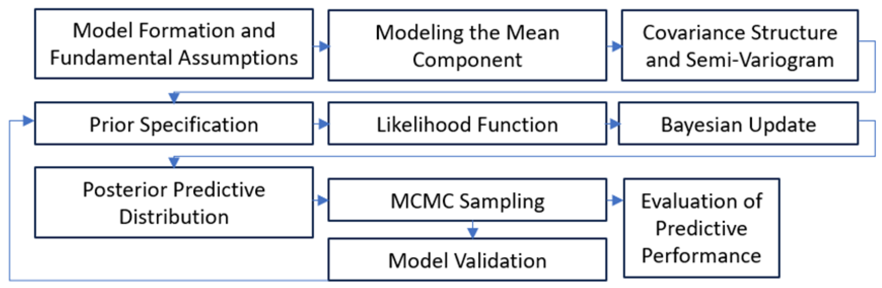
Figure 3.
Top panel -> left: Initial sparse grid of SST observations; right: Detail of the dense grid after densification. Bottom panel-> left: SST Bayesian Inference Prediction Uncertainty vs Initial Observations; right: Initial and Predicted SST values (in parentheses).
Figure 3.
Top panel -> left: Initial sparse grid of SST observations; right: Detail of the dense grid after densification. Bottom panel-> left: SST Bayesian Inference Prediction Uncertainty vs Initial Observations; right: Initial and Predicted SST values (in parentheses).
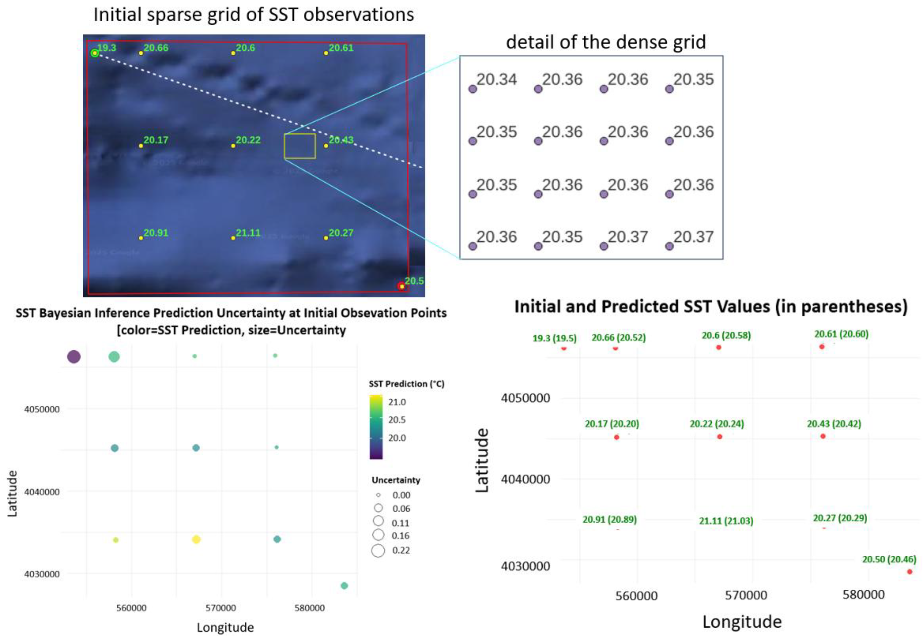
Figure 4.
Descriptive Statistics of Predicted Sea Surface Temperature (SST). Top panel -> left: Histogram of the predicted SST means (°C) across the study area, indicating the distribution of kriged estimates, center: Mean variance values grouped by SST zones (in 0.5 °C increments), quantifying the internal variability of SST predictions within each temperature class, right: Total variance contribution by SST zone, showing how different SST ranges contribute to the overall prediction uncertainty. Bottom panel-> left: Histogram of the predicted variances for SST, showing that the vast majority of prediction variances are low, reflecting high model confidence in most grid cells, right: Percentage of predicted mean SST values falling within each SST range, indicating the relative dominance of each temperature zone in the predicted spatial field.
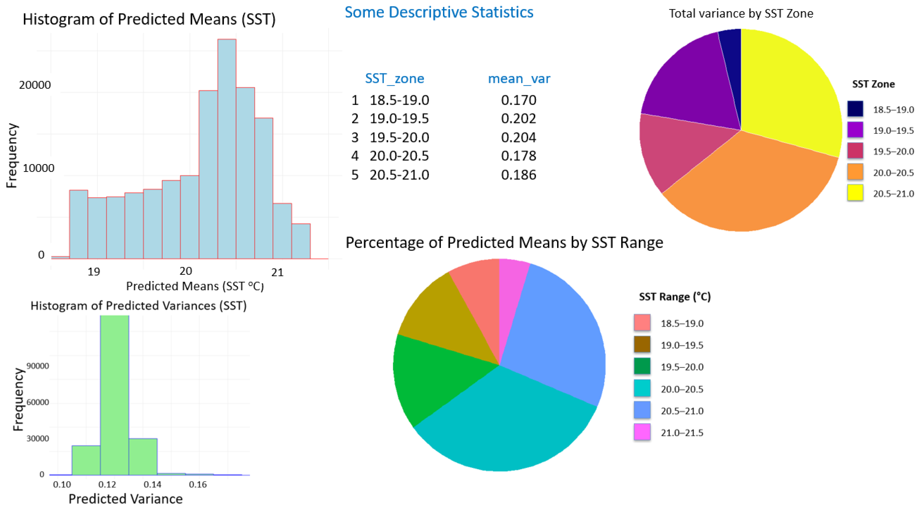
Figure 5.
Monthly Chlorophyll Concentration, March 2024 (La Spezia, Italy) -> Left: Initial chlorophyll grid (500×500m) from CMEMS and trajectory data, Right: Densified chlorophyll field (30×30m) using Bayesian kriging, Center: Study area location (Magra River estuary).
Figure 5.
Monthly Chlorophyll Concentration, March 2024 (La Spezia, Italy) -> Left: Initial chlorophyll grid (500×500m) from CMEMS and trajectory data, Right: Densified chlorophyll field (30×30m) using Bayesian kriging, Center: Study area location (Magra River estuary).
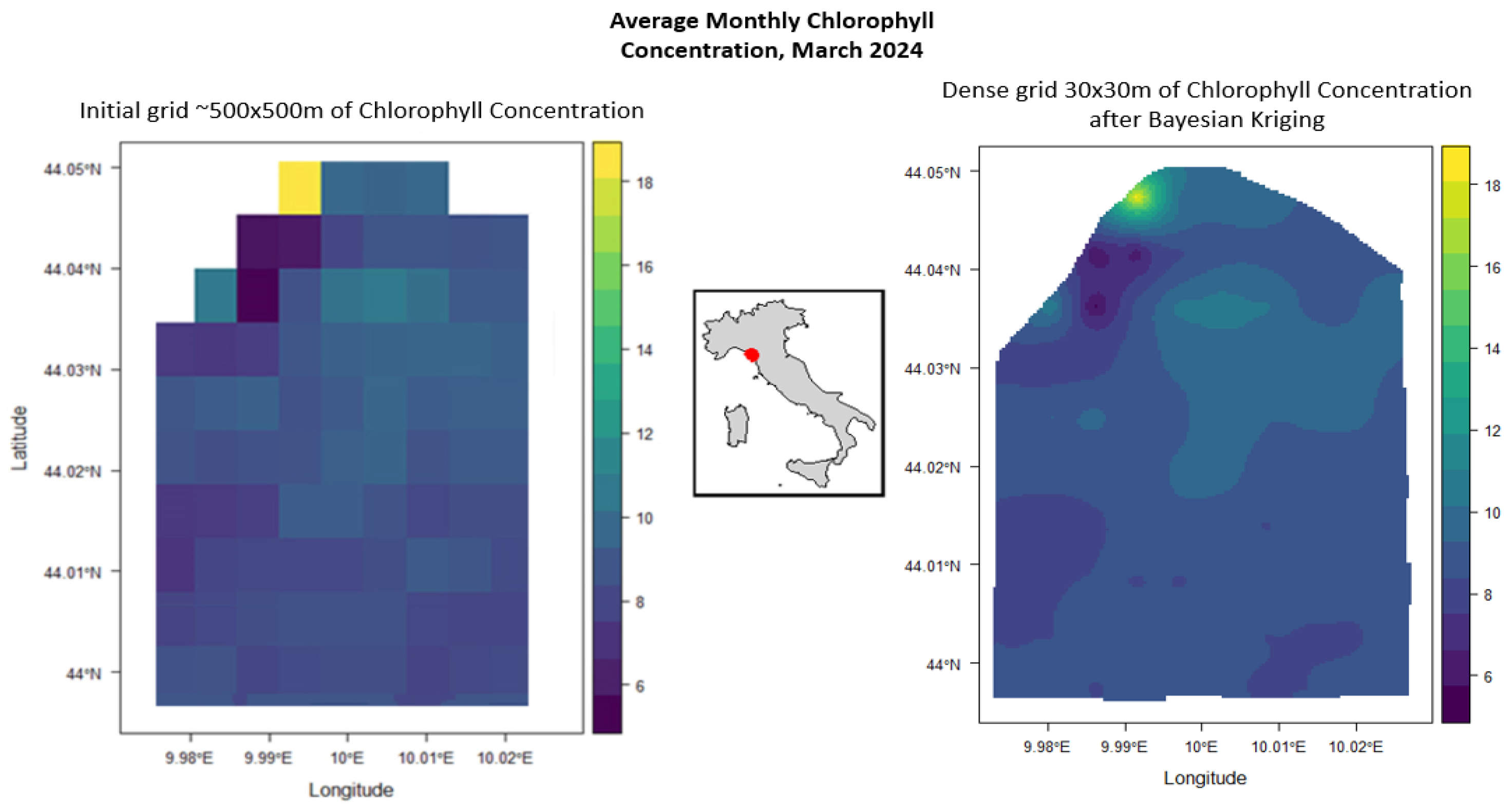
Figure 6.
Monthly Chlorophyll Concentration, September 2024 (La Spezia, Italy) -> Left: Initial chlorophyll grid (500×500m), Right: Densified chlorophyll field (30×30m) using Bayesian kriging, Center: Study area location (Magra River estuary).
Figure 6.
Monthly Chlorophyll Concentration, September 2024 (La Spezia, Italy) -> Left: Initial chlorophyll grid (500×500m), Right: Densified chlorophyll field (30×30m) using Bayesian kriging, Center: Study area location (Magra River estuary).
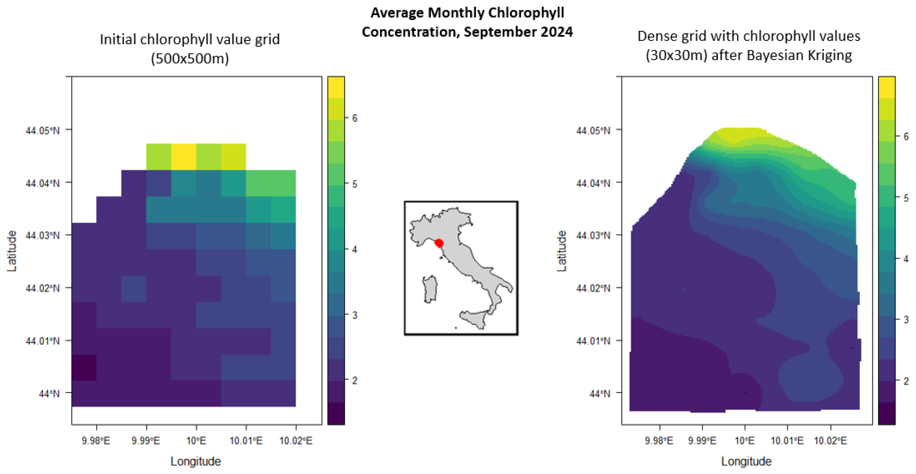
Figure 7.
Behavior of MCMC Chains for Bayesian Kriging parameters with trace plots and posterior density estimates for the MCMC sampling of key model parameters (σ², τ², ϕ, n) during Bayesian kriging of chlorophyll data. The left columns show results for March 2024 and the right columns for September 2024.
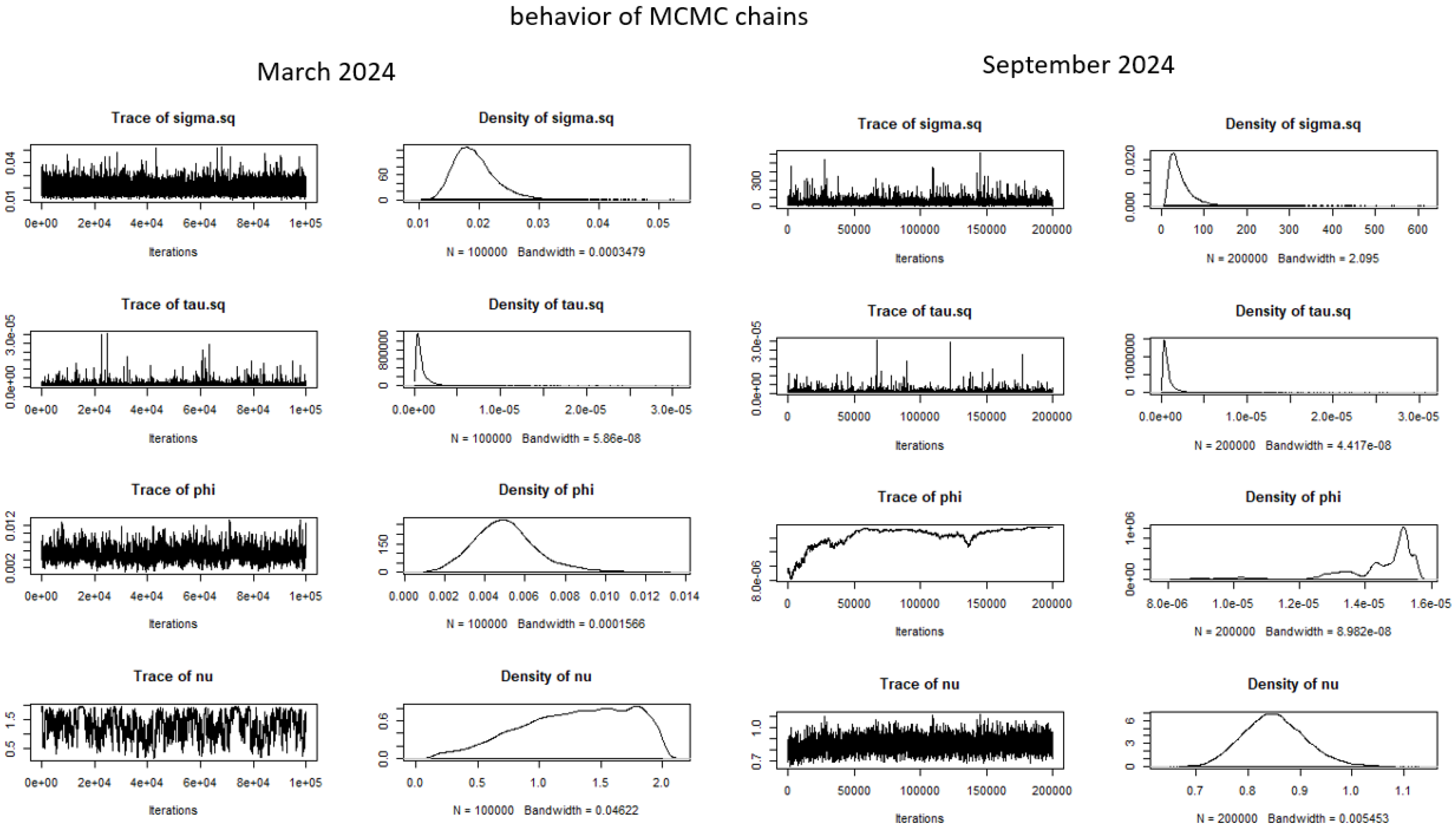
Figure 8.
Initial and Predicted Chlorophyll Concentration Values, March and September 2024 -> Grid comparison of observed and predicted (in parentheses) monthly average chlorophyll concentrations (red points, mg·m⁻³) over the coastal area near the Magra River estuary. The left panel shows values for March 2024, while the right panel corresponds to September 2024.
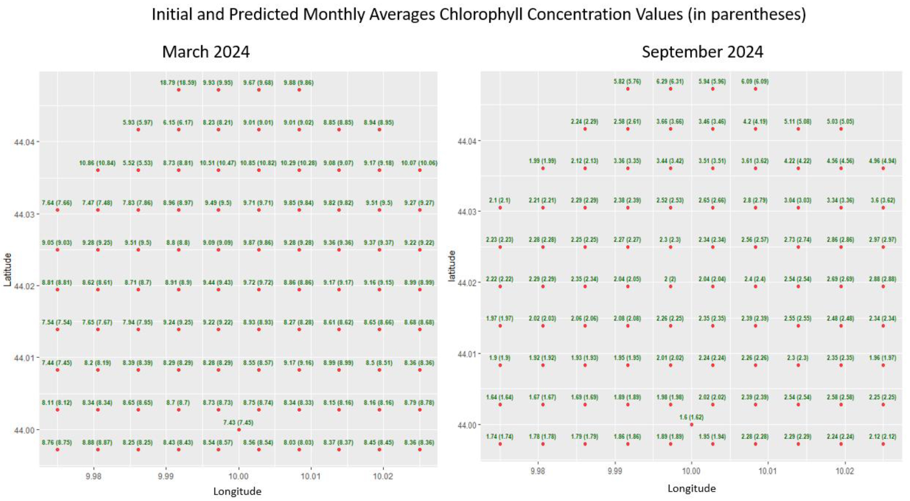
Figure 9.
Residual maps showing the spatial distribution of prediction errors (predicted minus observed chlorophyll concentration) for March (left) and September (right) 2024. Red tones indicate overestimations, while blue tones indicate underestimations.
Figure 9.
Residual maps showing the spatial distribution of prediction errors (predicted minus observed chlorophyll concentration) for March (left) and September (right) 2024. Red tones indicate overestimations, while blue tones indicate underestimations.
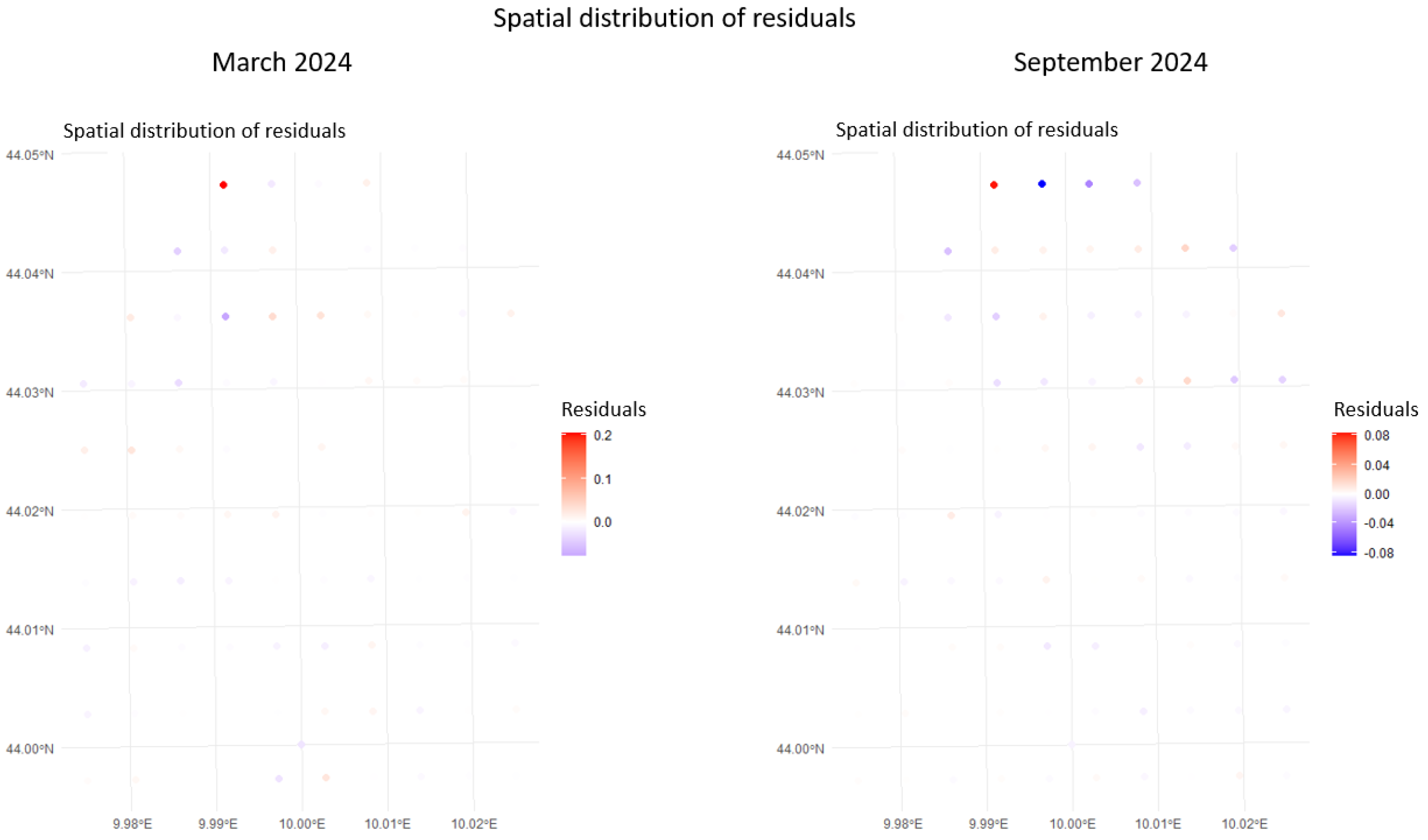
Figure 10.
Boxplots showing the distribution of chlorophyll concentrations (mg·m⁻³) across six distance zones from the coastline: 0-100m, 100-200m, 200-500m, 500m-1km, 1-2km and >2km. The left panel corresponds to March 2024 and the right panel to September 2024. A clear decreasing trend in chlorophyll concentration is observed with increasing distance from shore, particularly pronounced in March, likely due to stronger riverine nutrient input. This pattern reflects the influence of terrestrial runoff on nearshore productivity.
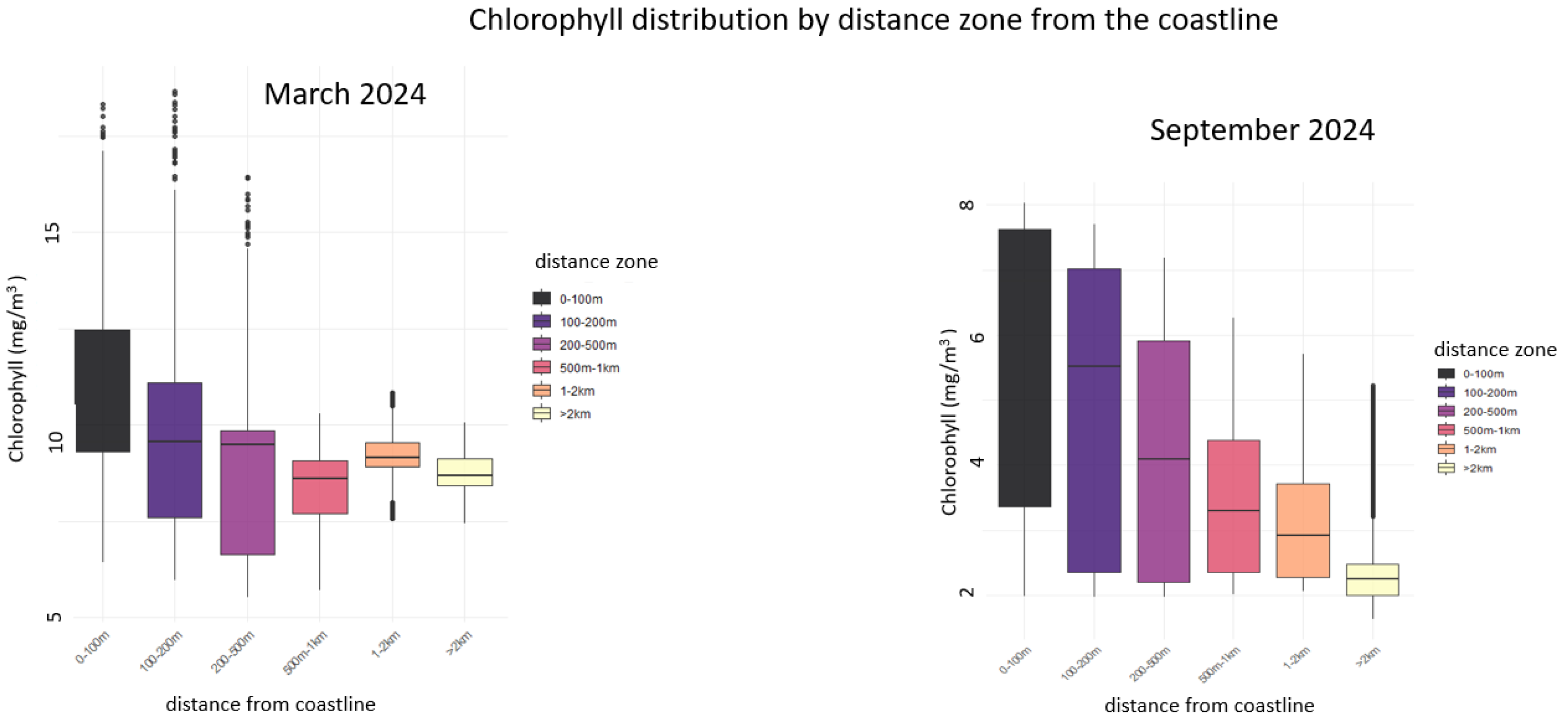

Table 1.
Εstimated uncertainty of the bayesian kriging model in the data scale (°C).
| Statistic | Estimated uncertainty (°C) |
| Min | 0.010 |
| 1st Qu. | 0.022 |
| Median | 0.091 |
| Mean | 0.101 |
| 3rd Qu. | 0.160 |
| Max | 0.221 |
| SD | 0.062 |
Disclaimer/Publisher’s Note: The statements, opinions and data contained in all publications are solely those of the individual author(s) and contributor(s) and not of MDPI and/or the editor(s). MDPI and/or the editor(s) disclaim responsibility for any injury to people or property resulting from any ideas, methods, instructions or products referred to in the content. |
© 2025 by the authors. Licensee MDPI, Basel, Switzerland. This article is an open access article distributed under the terms and conditions of the Creative Commons Attribution (CC BY) license (http://creativecommons.org/licenses/by/4.0/).
Copyright: This open access article is published under a Creative Commons CC BY 4.0 license, which permit the free download, distribution, and reuse, provided that the author and preprint are cited in any reuse.


