Submitted:
08 July 2025
Posted:
09 July 2025
You are already at the latest version
Abstract
Monitoring lakes is essential to understand their metabolism, guide management strategies, and contribute to the understanding of climate change, as these environments act as biomarkers. This study aims to propose an environmental assessment of Água Preta Lake, a shallow Amazonian Lake located in an urban area, through the three-dimensional modeling of hydrodynamics and sediment transport. The simulations, performed with the DELFT3D-FLOW model, used meteorological and physical data from the lake as boundary conditions. The results showed good statistical indicators, providing evidence of the model's reliability. Since it is a shoal lake fed by intense discharge with a high sediment load, this input directly influences the lake's circulation, promoting the resuspension of sediments and the redeployment of nutrients in the water column. This process increases water turbidity, alters the dynamics of biota, favoring the dominance of phytoplankton and floating macrophytes, which contributes to eutrophication and reduced water quality. The study emphasizes the importance of continuous surveillance, managing anthropogenic influences, and implementing restoration efforts to prevent the progressive degradation of urban lake ecosystems.
Keywords:
lake hydrodynamics
; sediment resuspension
; thermal stratification
; limnology
; Delft3D
1. Introduction
Lakes are ephemeral environments in the Earth's landscape, characterized by their short duration on a geological scale. The decline of these environments is intrinsically linked to their own metabolism, such as the accumulation of organic matter in sediment and the deposition of sediments carried by inflows [1].
The sedimentary dynamics and water quality of these systems are intrinsically linked to hydrodynamic parameters and their circulation patterns. This complex relationship is best seen in shallow tropical wind-driven lakes [2], since these water bodies are too shallow to develop thermal stratification, and are subject to more frequent sediment resuspension events, due to the action of currents generated by wind shear on the lake surface [3,4,5]. Such resuspension interferes with various aspects of lake metabolism, e.g., increasing nutrients and turbidity in the water column, limiting the zone of primary productivity, leading to the dominance of planktonic organisms [6,7] and floating macrophytes on the lake surface [6,7,8,9].
These shallow lakes may have less resilience than the larger and deep ones, making them more vulnerable to pollution and processes of eutrophication [10], in other words, they are more sensitive to interference in their metabolism, which accelerates their disappearance [9].
Which, in turn, may be inserted in large urban centers, being able to control air temperature and humidity, two major factors that generate health comfort for urban life. It can mitigate the processes associated with climate change in these areas, such as extreme heat islands in urban centers, causing morbidity and mortality [11,12]. Furthermore, urban lakes perform numerous ecosystem services, such as water supply for domestic and industrial activities [13,14,15], maintenance of biodiversity in this ecosystem [10,16,17,18], adjustment of the urban microclimate[11,12,19,20].
Nestled in the Brazilian Amazon lies the capital of Pará, Belém, a large urban center with a population of 1,303,403 people, making part of the Belém Metropolitan Region (BMR). [21]. Development in the capital has been rapid and disorganized, putting pressure on nearby urban ecosystems. [22].
With that in mind, one of the few green areas in the capital is the Utinga State Park, which is home to two Amazonian lakes (Bolonha and Água Preta) supplying RMB, located between the municipalities of Belém and Ananindeua. It is important to note that the lakes are located in an urban context, surrounded by residential areas and highways, reflecting the rapid and disorderly urbanization of the municipalities that encompass the lakes. As such, they are subject to anthropogenic impacts.[17,23,24]. Building on the concept of lakes disappearing due to their metabolism, several studies show that the Utinga lake system is going through a process of silting, pollution, and eutrophication. [25,26,27].
Life quality in urban centers is directly impacted by the presence and health of these lake environments, which can help preserve biodiversity [10,28,29], restore natural resources [10,28,30,31], mitigate the urban climate [10,11,32,33], supply of drinking water for domestic and industrial activities [34], conservation of green areas [33,35], and recreational and educational activities [22,34,35].
Developing three-dimensional numerical models is super important for learning about lake dynamics, especially hydrodynamics and sediment transport, and these models can simulate across different time and space scales. That said, lakes are defined as slow-moving or still environments, in which studies tend to use one-dimensional vertical models that only show how properties change along the water column[36,37]. This approach, although useful in certain contexts, limits the spatial and temporal analysis of processes, compromising a more comprehensive understanding of lake dynamics [37]. Similarly, in the field of study, where research focuses on two-dimensional hydrodynamic models [38,39].
In spite of this approach to the low energy of lakes, these ecosystems have complex bathymetry and topography, able to infer directly on hydrodynamics and substance transport patterns. This highlights the need to apply three-dimensional models that can more accurately represent physical interactions in these environments [40].
In this study, there is a focus on understanding the hydrodynamic and morphodynamic processes of Água Preta Lake in order to monitor the changes undergone by this environment using three-dimensional numerical modeling (Delft3D Flow). By highlighting the sedimentation and erosion parameters in the lake and developing a diagnosis and prognosis of the lake's hydro-sedimentary dynamics, we seek to gain a new perspective on Lake Água Preta.
2. Materials and Methods
2.1. Study Area
Água Preta Lake lies within an Environmental Protection Area (APA), surrounded by the urban environment of the city of Belém, called Utinga State Park. It is an APA (Environmental Protection Area), created with the main purpose of preserving the potability of the waters of the Bolonha and Água Preta lakes, also providing a space conducive to leisure and the development of ecological and scientific activities [41]. These two lakes form a lake system that supplies 65% of the city of the BMR.
The lake system was engineered to function as a potable water reservoir for the BMR. The inflow and outflow are regulated by the Pará State Sanitation Company (COSANPA), which controls routing through the system to ensure continuous supply to the water treatment facility.
Thus, it can be said that the system is formed by three large water bodies: the Guamá River, Água Preta Lake and Lake Bolonha (Figure 1). To keep the water level constant, COSANPA uses the Guamá River as a water inlet to the Água Preta Lake (inflow), in which this artificial influx varies according to the seasonal periods, reaching 7 m³/s in the dry periods and 3 m³/s in the rainy ones. After that, the water from Água Preta Lake flows into Bolonha Lake (outflow) through an artificial channel without pumping, which eventually reaches the treatment plant.
In addition, Água Preta Lake is classified as a shallow lake, with a maximum depth of 4 meters, and small in size, approximately 7.2 km², resulting in a volume of approximately 9,905,000 m³ [41,42]. Given this, there is great concern about the inflow of the Guamá River into the lake, since the Guamá River has a high suspended sediment load [43]. These suspended sediments are transported to the lake which, in turn, sediment in its bed, accelerating silting processes.
The meteorological parameters of the region have particular features in relation to the urban environment in its surroundings. Due to being an area of extensive vegetation cover, there is the formation of a local microclimate, which varies between two climatic zones Am and Af. Am is defined as a tropical climate with monsoons, and Af is the same as the city of Belém [41], which would be a climate belonging to the tropical class, without seasonal winter [44,45,46].
In this region, there are two seasonal periods: rainy season (December to May) and dry season (June to November). During the rainy season, rainfall originates from the Intertropical Convergence Zone (ITCZ), together with mesoscale effects, such as the lines of instability formed in northeastern Pará, which enter the region and are responsible for rainfall during the dry season [26,44].
2.2. Data Acquisition
PEUt has its own linimetric station that was implemented by the Observatory of the Amazon Coast – OCA in November 2023. Therefore, part of the parameters used in the simulations were from this station and the Belém station, 3 km away from Água Preta Lake (Figure 1), monitored by the National Institute of Meteorology (INMET). In which both stations collect meteorological data at the same height, i.e., 2 meters above the surface where the station is fixed.
The input data were primarily meteorological, including air temperature ( C), relative humidity (%), wind speed and direction (m/s), obtained by the OCA station, while solar radiation (J/m².s), precipitation (mm/day), and cloud cover (%) data were obtained from the INMET station for the period from November 2023 to October 2024 (Figure 2), period that covers the regio seasonal changes, dry and rainy seasons. To describe the morphology of the lake, a bathymetric survey of the lake was carried out, using an Echosonde coupled to a Garmin GPS, Chartplotter Echomap UHD 62CV model in November 2023.
The values for water inflow discharge (m³/s) were obtained by COSANPA, and these values were adapted so that the hydrodynamic simulations more accurately reflected reality (Table 1).
For the simulation calibration, a temperature time series was used. This data collected from a water level sensor, Solinist LevelLogger 5 model, installed on the A17 (February 2024).
The simulation was later validated through temperature profiles collected monthly with a CTD model SBE 19plus V2 SeaCAT Profiler, at 19 points of the lake, with a sampling rate of 4 Hz. In addition, two time series of currents obtained from an INFINITY-EM current meter were used, with measurements taken at points A08 and A13 (Figure 3), 0.5 m above the lake bed, for one day.
Temperature was the main parameter used in the calibration and validation of the lake's hydrodynamics, since the body of water has a controlled and constant level throughout the year, as well as slow circulation, with a maximum speed of approximately 0.31 m/s [39], subject to rapid fluctuations in direction. As such, temperature responds to variations in circulation and water quality parameters and is widely used in the calibration and validation of hydrodynamic and water quality simulations in shallow lakes. Prior studies have demonstrated this approach in different lake systems, such as Otter Lake, Minnesota, USA [47], Lake Okeechobee, Florida, USA [48], and Créteil, Paris, France [49].
2.3. Model Description
The simulations were developed using the Delft3D-Flow (D3D) model, a numerical model capable of solving nonlinear differential equations in a discretized domain [50]. For the purpose of forcing movement in the simulated fluid, the model utilizes external forces to generate a flow circulation pattern, depending on the force.
This model was chosen for its comprehensive scope, presenting satisfactory results in the validation of hydrodynamic models of deep lakes [51], shallow lakes [52], and urban lakes [49].
2.3.1. Heat Flux Model Description
Heat flux model 1 (absolute flux, total solar radiation) intrinsic to the D3D model was used for the simulation. These components of the heat balance are calculated by D3D using a free surface area. [50,53]. The heat balance is determined based on incident radiation, return radiation, evaporation, and convection, as in equation (1). Vaporization and convection are processes influenced by air and water temperature, relative humidity, and wind speed. These variables are used as input data in the simulations of Água Preta Lake.
In this equation, the heat balance at the air-surface interface is solved by considering the main components of energy exchange. A total heat flux (J/m²s) is determined by the sum of the contributions of different fluxes: , net incident solar radiation (short waves); , net incident atmospheric radiation (long waves); , back radiation (long waves emitted by the surface); , evaporative heat flux (latent heat); and , convective heat flux (sensible heat). In this way, the heat balance considers both energy gains and losses through different exchange mechanisms, with net solar radiation being one of the main sources of heat input into the system.
By using the total heat flow, we calculate the heat flow on the free surface of the body of water. Thus, it is possible to calculate the temperature variation of the lake surface and, by continuity, the temperature in the deeper layers, as in equation (2).
Here, assuming that the heat flow model neglects heat exchange with the bottom, the model may lead to an overestimation of water temperature, especially in shallow areas, as in our case study. Given this, it follows that is the specific heat capacity of seawater (=3930 Jkg-1 K), is the specific density of water (kg/m³), and is the thickness of the upper layer (m).
2.3.2. Morphodynamics and Sediment Transport Module Description
The D3D sediment transport module uses two types of sediments, cohesive and non-cohesive. For this study, cohesive sediments type was used, defined as silt and/or clay, which are common in low hydrodynamic environments, such as lakes. This module incorporates transport, erosion, and deposition in the simulations.
For the transport of suspended sediments in three dimensions, it is calculated from the solution of the mass balance equation for suspended sediments [50,54], described by the equation (3):
In this equation, is the mass concentration of sediment fraction i (kg/m³), terms , and are turbulent diffusivities of the sediment fraction in the x, y, and z directions (m²/s), u, v, and w are components of the flow velocity in the x, y, and z directions (m/s), and is the sedimentation velocity of the sediment fraction (m/s).
Bathymetry of the water body is overwritten at each time step based on changes in suspended and bottom sediment loads, multiplied by the morphological scaling factor (MORFAC), which can accelerate the morphological processes of the simulation[50,55]. First, the sediment load variation (Mb) on the bed is calculated using the equation (4), in order to solve the bathymetry update in the equation(5).
where, Mb is the integrated sediment mass in the bed (kg/m²), MORFAC is the morphological scaling factor, and are the bottom sediment loads (in x and y) transported by the currents, zb is the variation in bed level, p is the porosity, or water fraction of the total bed volume, and ρ is the specific density of the sediment (kg/m³).
2.3.3. Configuration and Parameterization of Simulation Input Variables
The simulations took place from November 2023 to September 2024, at a time step of 1 minute. This period was chosen with the intention of covering the dry and rainy periods that govern the seasonality of Lake Água Preta. Also, changes were made to the meteorological data for winds and solar radiation.
Since the D3D heat flux model 1 considers cloudiness as a constant parameter, this parameter was modeled for use in the simulations (75%). However, since we are dealing with an Amazonian region, i.e., one with high cloudiness, it was necessary to multiply the solar radiation by 1.8 so that the simulations would more accurately represent the actual data.
For wind data, it was verified that the input data for D3D must be 10 meters from the surface (U10). Therefore, the equation described by [56] was applied, which assumes a logarithmic behavior of the wind intensity profile, where its speed increases with height, also taking into account the roughness of the ground or degree of obstruction.
The wind measurements taken by the AP weather station occur on land, and not directly over the lake surface. For this reason, a correction factor of 1.5 was applied to the wind magnitude, as proposed by [57] and [58], in order to more accurately represent the conditions on the water surface in hydrodynamic models. This correction takes into account the difference in surface roughness between soil and water, which affects wind intensity near the surface, as described by [32] In the simulations, the value entered for the wind drag coefficient was 0.003 according to [59], which adjusts the drag coefficient, assuming an empirical value of 0.003 for shallow and wide lakes.
The Água Preta Lake domain was discretized into a structured mesh, with 20x20 m elements and 10 vertical sigma-type layers (Figure 1), , i.e., varying in size according to bathymetry and free surface [50]. At the free surface boundary of the simulated domain, the movement is generated by the wind shear stress on the water surface, and the magnitude of the shear stress is defined in equation (6) as:
where is the magnitude of wind shear stress, is air density, and is the wind drag coefficient, dependent on .
At the inflow boundary, the time series provided by COSANPA was used, where a multiplication factor of 5 was applied so that the simulations would better reflect the actual data. The water temperature and sediment load entering the system were empirically assumed to be 29ºC and 0.2 kg/m³, respectively.
Since we assumed that the lake level is constant during the simulation period, the outflow limit was set as the water level, where the water level is constant throughout the simulation period, thus behaving as a response limit to the inflow.
The bottom roughness values were discretized in the simulation domain, determined from the calculation of the Manning coefficient. Using the methodology described by [60], which takes into account the granulometric characteristics of the bottom sediment, the type of vegetation, and the degree of obstruction of the water body [61], to determine roughness. After discretizing the roughness by the particularity of the areas present in the domain, the roughness values were interpolated in the domain, as described in Table 2
Four statistical metrics were applied in the model calibration stage: (i) root mean square error (RMSE) to analyze the difference between the modeled and actual data; (ii) Pearson's correlation (r) to estimate the behavior between the actual and predicted data; (iii) the coefficient of determination (R²) to test the efficiency of the model; (iv) and the maximum absolute error (MAE) to quantify how much the simulation differs from the observed data. These metrics are commonly used for the validation and calibration stages of lake environment simulations [35,49,51,62,63,64].
3. Results and Discussion
3.1. Calibration
During the calibration stage at point A17, the statistical metrics related to the temperature curves (RMSE = 0.27 C and MAE = 0.87 C) show that the simulation accurately represents the ambient temperature (Figure 4).
Therefore, the MAE index must be less than 20% of the maximum annual variation in lake temperature [62], which is satisfied by the simulations.
Therefore, in the case of Lake Água Preta, which has minimum temperatures of 25 ºC and maximum temperatures of 34 ºC during the rainy season (February to April) and on sunny days during the dry season (July to October), the MAE and RMSE values cannot exceed 2.0 ºC.
The Pearson (ρ = 0.89) and coefficient of determination (R² = 0.79) values also presented good metrics when representing the actual data, where, in addition to the correlation coefficient, when performing a regression curve, it is possible to verify that the temperature values have a strong positive correlation (Figure 4).
3.2. Model Validation
For the velocities at points A08 and A13, in order to compare the actual and simulated data, only the RMSE and Pearson tests were used, where the points presented RMSE of 0.009 m/s and 0.012 m/s and ρ of 0.1 and 0.5, respectively. As previously stated, these statistical metrics are low, which is expected in shallow lake simulations, as they present lenthic flow. That said, they are unstable flow environments, subject to rapid changes in velocity due to wind gusts and rain [52,64]. In addition, Água Preta Lake has tall trees on its banks that obstruct wind flow, resulting in a slight overestimation of velocity values (Figure 5).
When comparing the simulated and observed temperature profiles from points A01 to A19, it was possible to verify that the largest errors in the simulation are found at points A01, A09, A11, and A19 (Table 3). There were special cases where the validation metrics were low. At points A01, A03 in December, and A17 in June. Floating macrophytes tended to settle in these regions of the lake. As a result, the lake surface in these locations was covered by this vegetation, resulting in changes in the temperature profile behavior in these locations. These uncertainties are associated with local anthropogenic changes and variables not included in the simulations.
Sampling points confined to or close to the margins are subject to local influences that can alter temperature dynamics through the discharge of domestic effluents, tree canopies, and small local springs. This is the case at points A01 and A19, located at the northern ends of the lake, where the greatest temperature differences occur (There were special cases where the validation metrics were low. At points A01, A03 in December, and A17 in June. Floating macrophytes tended to settle in these regions of the lake. As a result, the lake surface in these locations was covered by this vegetation, resulting in changes in the temperature profile behavior in these locations). These points are located in sheltered and morphologically funneled regions, keeping the site shaded by tree canopies during the day. In addition to being located adjacent to the urban environment, they are subject to the discharge of domestic effluents.
Points A09 and A11 are the closest points to the lake's inflow point, which explains the lower correlation indices at these points (There were special cases where the validation metrics were low. At points A01, A03 in December, and A17 in June. Floating macrophytes tended to settle in these regions of the lake. As a result, the lake surface in these locations was covered by this vegetation, resulting in changes in the temperature profile behavior in these locations). This is because the artificial supply of water has the capacity to disrupt the hydrodynamics of the system. This alters the circulation patterns previously established naturally in the system, resulting in changes in temperature and possibly in water quality parameters.
There were special cases where the validation metrics were low. At points A01, A03 in December, and A17 in June. Floating macrophytes tended to settle in these regions of the lake. As a result, the lake surface in these locations was covered by this vegetation, resulting in changes in the temperature profile behavior in these locations.
3.3. Setorização
To organize the presentation and discussion of the simulation results, the domain was divided into three areas according to the particularities of each zone, namely: West, the portion influenced by inflow and outflow; Central, the location that directly receives the inflow, with the most intense water flow in the system and the deepest regions of the lake; East, the most controlled portion of the lake, without a water inflow or outflow system (Figure 6).
Observation points A07, A10, and A16 were selected to represent the western, central, and eastern portions, respectively. This enables an understanding of the stratification patterns over time in the system.
3.4. Circulation Patterns of Água Preta Lake
Given the lentic nature of lakes, the flow present in this environment is of low magnitude, primarily resulting from the action of wind on surface waters, presenting a logarithmic vertical profile [66].
Figure 7 shows the surface and bottom circulation pattern of Água Preta Lake between February (rainy) and June (dry) 2024. These months were chosen because they represent seasonality, and according to [39], which shows that February and June are the months with the lowest and highest speeds, respectively.
The average surface velocity ranged from 0 m/s to 0.19 m/s and, at the bottom, from 0 to 0.15 m/s. From this, it was observed that the domain has low velocities throughout, with maximum velocities associated with inflow and outflow.
The inflow waters enter the lake through a funnel-shaped channel until it reaches the central region. This flow is slowed down when it encounters the domain waters, characterized by being slower than the channel flow, resulting in directing the inflow waters to deeper layers [14]. This circulation forms currents in the central region that behave similarly to a vortex, highlighting the locations that tend to have greater sedimentation. In the outflow, the artificial channel between the Água Preta and Bolonha lakes increases the magnitude of the currents, explained by the difference in elevation between these areas, which can reach 6 m, culminating in gravity flow [38].
The recorded values show that the rainy season has lower average speeds when compared to the dry season, due to the local wind pattern and the morphological characteristics of the lake (Figure 7). Winds in the region are stronger during periods of low precipitation due to the influence of the Intertropical Convergence Zone in the region [44]. In addition, Água Preta Lake has a large fetch region, resulting in higher current speeds during the dry season, since wind is one of the controlling agents of the current field in lake systems.
In the eastern region, without the influence of inflow and outflow, the average surface and bottom currents have speeds of 0.008 m/s and 0.001 m/s, respectively. In the central and western regions, the average speeds are higher, at 0.02 and 0.009 m/s at the surface and 0.016 and 0.013 m/s at depth. The western region shows a peculiar flow in relation to the other sections, forming a constant flow at depth, which connects the inflow and outflow points (Figure 7).
This constant flow, occurring at the bottom of the lake, can promote the resuspension of sediments and organic matter along the analyzed stretch. This process can result in the release of substances previously unavailable in the water column due to their entrapment in sediments, such as nutrients, which can be assimilated by local organisms, such as macrophytes, favoring their development [1]. In addition, resuspension can release gases from the decomposition of organic matter and influence physical-chemical parameters such as pH, dissolved oxygen, and redox potential [19].
In general, no significant variations in horizontal circulation patterns were observed between the periods analyzed. In June, speeds greater than 0.005 m/s were recorded in a larger portion of the domain, possibly associated with increased wind intensity and the predominance of winds from the north (10º-15º). On the other hand, the lower velocity values observed on the western side of the lake in February are attributed to the incidence of NNE winds (20º-25º) during this period. This influence is also a reflection of the morphology of the lake, which has north-south oriented corridors, expanding the area of action of winds from the north. In this context, the horizontal speeds of Lake Água Preta exhibited relatively uniform behavior throughout the simulated periods, with occasional variations in intensity throughout the seasons.
The maximum speeds of the lake occur at the surface, due to the action of the winds, which generate surface currents through turbulent stress, transmitting energy vertically through the interaction between adjacent layers of the water column. This energy dissipates progressively, so that the deeper layers are influenced by the substrate, resulting in a loss of speed due to friction generated by the flow in contact with the bottom [9,67,68]. This phenomenon gives rise to a vertical speed profile that resembles a logarithmic curve.
However, because it is a shallow lake with a maximum depth of approximately 4 meters, the attenuation of velocity in the deeper layers is less significant. Thus, when horizontal currents interact with the bed, a differential flow is formed at depth. This flow can have a magnitude similar to or even greater than that of surface currents, however, it tends to move in the opposite direction to the prevailing surface flow [9].
This phenomenon generates zones of minimal horizontal velocity, intensifying vertical velocity and promoting the resuspension of the surface layer of unconsolidated sediments. As a result, the water column is once again enriched with nutrients, altering water quality parameters such as turbidity and impacting the ecology of the lake. Increased turbidity reduces light penetration at depth, hindering the establishment of submerged macrophytes [9]. On the other hand, emergent species, adapted to the surface, can proliferate due to the increased bioavailability of nutrients in the water column. This process can favor excessive colonization of the lake by certain species, resulting in a possible imbalance in the food chain [30].
3.5. Temperature Patterns and Stratification
Figure 8 shows the expected pattern for a shallow lake located in an equatorial region. There is slight thermal stratification during the day, with an average difference of 0.1 ºC and a maximum of up to 2 ºC between the surface and the bottom. This stratification occurs between 12 p.m. and 2 p.m., when the highest daily temperatures and radiation indices are recorded. The greatest temperature differences are between day and night, with minimum temperatures of 29 ºC and maximum temperatures of 31 ºC. Throughout the simulated period between dry and rainy seasons, we have a maximum difference of up to 10 ºC, with a minimum of 26 ºC and a maximum of 36 ºC.
The lowest temperatures in the simulation occurred in February, due to the variation in air temperature and solar radiation incident on the lake surface (Figure 8). The month of June had the highest temperatures among the periods analyzed, resulting from the increase in temperature and solar radiation, promoting greater heating of the surface layers and, consequently, heat diffusion to greater depths (Figure 8).
The points located in the western (A08) and central (A10) areas have similar behaviors, showing more accelerated cooling at night since this area is wider and strongly influenced by the inflow, causing greater intensity in the circulation of this location. The eastern section (A16) showed lower temperatures than the other zones, as the influence of inflow is minimal in relation to the western and central zones, which, combined with the wind pattern of the system, coming from the NNE, moves the water to the other zones.
In the three sections of the lake, the absence of a well-pronounced thermocline was observed during the four months of analysis, remaining unstratified for most of the time, with minimal stratification during periods of greater solar intensity. In shallow lakes, winds have the capacity to mix the surface and bottom layers, resulting in total circulation between the layers. Between the dry and rainy seasons of 2024, there was no significant difference in wind intensity, only 10º in its direction from NE to NNE, so the stratification pattern is the same in both seasonal periods.
Thus, Lake Água Preta, according to its temperature pattern, is classified as a polymictic lake, with multiple daily circulations, a classification characteristic of shallow and large lakes [1].
February showed a practically homogeneous distribution pattern both horizontally and vertically, with average horizontal variations of 0.7ºC and vertical variations of 0.8ºC. In contrast, June showed some heterogeneity in the horizontal temperature gradients, with the highest average temperatures concentrated in the eastern arm of the lake, both at the surface and at depth.
In the central region, the inflow from the Guamá River generates a temperature gradient, where the closer to the inflow, the temperature tends to decrease by about 0.5 ºC. This occurs due to the simulation settings, where the water inflow was defined at a temperature of 29 ºC.
In the western zone of the system, a temperature gradient is formed from the inflow to the outflow, due to the lower velocities in the zone, which tend to transfer less heat between the layers. To the north of this section, the temperature decreases due to the increase in velocity that promotes heat exchange with the outflow currents, evidenced by colder waters leaving the simulation domain (Figure 9).
The occurrence of total daily circulation in the lake has several implications for its metabolism. This phenomenon allows the movement of substances and organisms that inhabit the environment. [69] demonstrates that phosphorus concentrations in the surface and bottom layers of Lake Água Preta have similar values, whereas lakes normally accumulate this element mainly in sediments [66]. This suggests the circulation of this nutrient in the water column, which is made possible by the thermal destratification of the lake, leading to greater availability of this substance.
This process can therefore contribute to eutrophication through the constant circulation of nutrients. It also influences the permanence of potentially toxic metals in the water column, which are found in sediments located on the banks near the lake's occupied areas [70,71].
Based on this temperature dynamic, it is possible to state that Água Preta Lake fits the pattern of polymictic lake environments, i.e., they stratify several times during the year. In addition, through the hydrodynamic behavior of the lake, the system presented circulation predominantly dominated by the action of winds, with opposite flows between the surface and the bottom (reverse flow), a phenomenon characteristic of shallow and wide lakes, dominated by the intensity and direction of the winds [9].
The simulations showed a sectorization of the lake due to the hydrodynamic particularities of each sector. The Central and Western sections are strongly influenced by the artificial pumping of water into the lake, modifying the circulation and temperature of the system. The Eastern sector has more homogeneous flow and temperature gradients, reflecting variations in wind intensity and direction.
The Central and Western sectors, influenced by artificial pumping from the Guamá River, have a rich suspended sediment load that increases their turbidity. This phenomenon can cause possible impacts on the system's metabolism, such as the unavailability of light, the excessive increase of suspended nutrients (which can generate eutrophication, mainly on the lake's shores), and the disappearance of submerged vegetation when critical turbidity is reached, resulting in a murky lake dominated by phytoplankton [6,31].
When a lake reaches a critical point of turbidity, it becomes resistant to restoration alternatives, hindering water clarification processes, such as the establishment of submerged macrophytes that reduce turbidity and prevent sediment resuspension [6,31,72]. The change in turbidity can result in toxic algal blooms, odor, and significant loss of ecosystem services, such as water portability [31,73].
3.6. Transport and Sedimentation of Lake Água Preta
In Figure 10, it can be observed and confirmed that in both the dry and rainy seasons, sediment transport occurs mainly through the Guamá River's inflow into Lake Água Preta.
This sediment load from the system's inflow tends to flow from the central sector to the western sector due to the current formed between the inflow and outflow points, resulting in the western side of the lake having more turbid waters than the eastern side. Between seasonal periods, there is no significant difference in transport. However, there is a slight contrast in the way the sediments tend to spread. In June, due to the increased intensity of the lake currents, the sediment load tends to concentrate more in the central region, as the velocity vectors of the lake coming from the north push the sediment load towards the central region. However, in February, this speed decreases, which allows for greater spreading of these suspended sediments. This can be observed at the tip of the transport cloud in the easternmost region, where in February, transport tends to be directed slightly more to the east.
Based on the sediment transport occurring in the domain, it was possible to verify the difference between the bathymetries, highlighting the locations where the greatest sediment deposition occurs in the lake. The areas with the most significant accumulation are predominantly concentrated in the central region of the lake. These vary, with local sediment accretion that may reach up to approximately 0.30 m, especially in the area near the Guamá inlet. In addition, the lake, considering its entire domain, received an average elevation of 0.05 m.
This deposition is associated with the behavior of the inflow, which has a high sediment load and high velocities compared to the rest of the system. Upon entering the lake, this flow slows down considerably, reducing its sediment transport capacity. As a result, preferential deposition occurs in the central region, especially near the inflow entry point, where the energy of the flow is dissipated more quickly.
4. Conclusions
Three-dimensional numerical modeling was developed using Delft3D for Água Preta Lake, simulating the lake's circulation and sedimentation patterns. The simulations showed good results in calibrating and validating the temperature both over time and in spatial differences in the system. The greatest disparities in the calibration metrics were due to the particularities of each point.
Água Preta Lake did not show large seasonal variations in temperature and velocity. However, the dry season showed higher temperatures and velocities in the lake as a whole. Due to the region being equatorial, that is, subject to slight temperature fluctuations, these variations are small. As the lake studied has shallow depths and is subject to intense solar radiation throughout the day, the temperature showed a maximum difference of 2 ºC between the surface and the bottom. The phenomenon of reverse flow was also observed in the lake, given as a deep flow that has the opposite direction to the surface flow.
Under natural conditions, the lake is mainly dominated by the action of the winds. However, based on the sectorization of the lake, the central region showed that the intense artificial inflow of the Guamá River into the system has the capacity to alter the circulation and sedimentation parameters of the lake. This process increases turbidity and the sedimentation rate in the vicinity of the inflow, which may lead to future degradation of the lake's water quality, re-releasing nutrients into the water column and decreasing the rate of light entering the lake.
This can result in a system equilibrium of a turbid lake dominated by phytoplankton, reducing the amount of submerged macrophytes in the environment that serve to regulate water color and transparency. This indicates that Água Preta Lake needs more monitoring projects, given its importance to the Belém metropolitan area, promoting ecosystem services, regulating the local climate, and providing drinking water. Some preventive measures to reduce the turbidity of this environment would be the implementation of submerged macrophytes as well as better regulation of the sediment load that artificially enters the lake.
Therefore, based on the diagnosis of Água Preta Lake, which highlights the need for further studies on the lake's water quality, numerical modeling should also be applied as a tool to predict new solutions for monitoring this lake that supplies the city of Belém.
Author Contributions
M.C: writing, conceptualization, investigation, field data acquisition, data curation, graphic design, chart creation, and visualization; A.Q: writing – methodology, investigation, chart creation; and M.R.: conceptualization, supervision, and funding acquisition. All authors have read and agreed to the published version of the manuscript.
Funding
This research was funded by the State Secretariat for the Environment and Sustainability – SEMAS Pará – and a master scholarship granted by Coordination for the Improvement of Higher Education Personnel -CAPES-.
Data Availability Statement
The data presented in this study are available on request from the corresponding author.
Acknowledgments
The authors gratefully acknowledge Thais Borba from the Marine Environmental Monitoring Research Laboratory, Federal University of Pará, for her professional support in numerical modelling interpretation.
Conflicts of Interest
The authors declare no conflicts of interest.
References
- Esteves, F.A. 1998. Fundamentos de limnologia. Interciência.
- Liu, S.; Ye, Q.; Wu, S.; Stive, M.J.F. Horizontal Circulation Patterns in a Large Shallow Lake: Taihu Lake, China. Water 2018, 10, 792. [Google Scholar] [CrossRef]
- Bailey, M.C.; Hamilton, D.P. Wind Induced Sediment Resuspension: A Lake-Wide Model. Ecological Modelling 1997, 99, 217–228. [Google Scholar] [CrossRef]
- James, R. Thomas.; Martin, J.; Wool, T.; Wang, P.F. A Sediment Resuspension and Water Quality Model of Lake Okeechobee. JAWRA Journal of the American Water Resources Association 1997, 33, 661–678. [Google Scholar] [CrossRef]
- Qin, B.; Zhang, Y.; Zhu, G.; Gao, G. Eutrophication Control of Large Shallow Lakes in China. Science of The Total Environment 2023, 881, 163494. [Google Scholar] [CrossRef]
- Scheffer, M.; van Nes, E.H. Shallow Lakes Theory Revisited: Various Alternative Regimes Driven by Climate, Nutrients, Depth and Lake Size. Hydrobiologia 2007, 584, 455–466. [Google Scholar] [CrossRef]
- Chung, E.G.; Bombardelli, F.A.; Schladow, S.G. Sediment Resuspension in a Shallow Lake. Water Resources Research 2009, 45. [Google Scholar] [CrossRef]
- Zhao, J.; Ding, W.; Xu, S.; Ruan, S.; Wang, Y.; Zhu, S. Prediction of Sediment Resuspension in Lake Taihu Using Support Vector Regression Considering Cumulative Effect of Wind Speed. Water Science and Engineering 2021, 14, 228–236. [Google Scholar] [CrossRef]
- Zhang, C.; Chen, L. A Review of Wind-Driven Hydrodynamics in Large Shallow Lakes: Importance, Process-Based Modeling and Perspectives. Cambridge Prisms: Water 2023, 1, e16. [Google Scholar] [CrossRef]
- Naselli-Flores, L. Urban Lakes: Ecosystems at Risk, Worthy of the Best Care. Materials of the 12th World Lake Conference, Taal 2007 2008, 1333–1337.
- Zhao, L.; Li, T.; Przybysz, A.; Liu, H.; Zhang, B.; An, W.; Zhu, C. Effects of Urban Lakes and Neighbouring Green Spaces on Air Temperature and Humidity and Seasonal Variabilities. Sustainable Cities and Society 2023, 91, 104438. [Google Scholar] [CrossRef]
- Jandaghian, Z.; Colombo, A. The Role of Water Bodies in Climate Regulation: Insights from Recent Studies on Urban Heat Island Mitigation. Buildings 2024, 14, 2945. [Google Scholar] [CrossRef]
- Schirpke, U.; Tasser, E.; Ebner, M.; Tappeiner, U. What can geotagged photographs tell us about cultural ecosystem services of lakes? Ecosyst. Serv. 2021, 51, 101354. [Google Scholar] [CrossRef]
- Koue, J. Modeling the Effects of River Inflow Dynamics on the Deep Layers of Lake Biwa, Japan. Environ. Process. 2023, 10, 62. [Google Scholar] [CrossRef]
- Jiang, M.; Brereton, A.; Beckler, J.; Moore, T.; Brewton, R.A.; Hu, C.; Lapointe, B.E.; McFarland, M.N. Modeling Water Quality and Cyanobacteria Blooms in Lake Okeechobee: I. Model Descriptions, Seasonal Cycles, and Spatial Patterns. Ecological Modelling 2025, 502, 111018. [Google Scholar] [CrossRef]
- Menchén, A.; Espín, Y.; Valiente, N.; Toledo, B.; Álvarez-Ortí, M.; Gómez-Alday, J.J. Distribution of Endocrine Disruptor Chemicals and Bacteria in Saline Pétrola Lake (Albacete, SE Spain) Protected Area Is Strongly Linked to Land Use. Applied Sciences 2020, 10, 4017. [Google Scholar] [CrossRef]
- Zhang, Z.; Li, J.; Luo, X.; Li, C.; Zhang, L. Urban Lake Spatial Openness and Relationship with Neighboring Land Prices: Exploratory Geovisual Analytics for Essential Policy Insights. Land Use Policy 2020, 92, 104479. [Google Scholar] [CrossRef]
- Cheng, X.; Qu, M.; Hu, Y.; Liu, X.; Mei, Y. Differences in Microbial Communities and Phosphorus Cycles between Rural and Urban Lakes: Based on Glyphosate and AMPA Effects. Journal of Environmental Management 2025, 376, 124577. [Google Scholar] [CrossRef]
- Mishra, J.; Parashar, D.D.; Kumar, D.R. Review of Planning Guidelines for Urban Lakes In India. Journal of Positive School Psychology 2023, 555–562. [Google Scholar]
- Xie, Q.; Ren, L.; Yang, C. Regulation of Water Bodies to Urban Thermal Environment: Evidence from Wuhan, China. Front. Ecol. Evol. 2023, 11. [Google Scholar] [CrossRef]
- IBGE Instituto Brasileiro de Geografia e Estatística (Brazilian Institute of Geography and Statistics) Cidades. Available online: https://cidades.ibge.gov.br/brasil/pa/belem/panorama (accessed on 30 June 2025).
- Hossu, C.A.; Iojă, I.-C.; Onose, D.A.; Niță, M.R.; Popa, A.-M.; Talabă, O.; Inostroza, L. Ecosystem Services Appreciation of Urban Lakes in Romania. Synergies and Trade-Offs between Multiple Users. Ecosystem Services 2019, 37, 100937. [Google Scholar] [CrossRef]
- Wei, G.; Yang, Z.; Liang, C.; Yang, X.; Zhang, S. Urban Lake Scenic Protected Area Zoning Based on Ecological Sensitivity Analysis and Remote Sensing: A Case Study of Chaohu Lake Basin, China. Sustainability 2022, 14, 13155. [Google Scholar] [CrossRef]
- Mishra, M.; Singhal, A.; Srinivas, R. Effect of Urbanization on the Urban Lake Water Quality by Using Water Quality Index (WQI). Materials Today: Proceedings 2023. [Google Scholar] [CrossRef]
- Andrade, A.L.C.; Tavares, P.A.; Santos, Y.R.; Brabo, L.D.M.; Ribeiro, H.M.C.; Beltrão, N.E.S. Diagnóstico ambiental dos impactos da proliferação de vegetação macrófita no lago Bolonha na cidade de Belém-PA. In Proceedings of the Blucher Engineering Proceedings; Editora Blucher: Belo Horizonte, Brasil, July, 2017; pp. 473–481. [Google Scholar]
- Oliveira, G. M. T. S. De., Oliveira, E. S. De., Santos, M. De L. S., Melo, N. F. A. C. De., & Krag, M. N... Concentrações de metais pesados nos sedimentos do lago Água Preta (Pará, Brasil). Engenharia Sanitaria E Ambiental 2018, 23, 599–605. [Google Scholar] [CrossRef]
- Castro, D.C.C. de; Rodrigues, R.S.S.; Filho, D.F.F. Surface runoff from drainage area of the lakes Bolonha and Black Water in Belém and Ananindeua, Pará. Research, Society and Development 2020, 9, e38932373–e38932373. [Google Scholar] [CrossRef]
- Wen, C.; Zhan, Q.; Zhan, D.; Zhao, H.; Yang, C. Spatiotemporal Evolution of Lakes under Rapid Urbanization: A Case Study in Wuhan, China. Water 2021, 13, 1171. [Google Scholar] [CrossRef]
- Xie, H.; Ma, Y.; Jin, X.; Jia, S.; Zhao, X.; Zhao, X.; Cai, Y.; Xu, J.; Wu, F.; Giesy, J.P. Land Use and River-Lake Connectivity: Biodiversity Determinants of Lake Ecosystems. Environmental Science and Ecotechnology 2024, 21, 100434. [Google Scholar] [CrossRef]
- Jin, H.; van Leeuwen, C.H.A.; Van de Waal, D.B.; Bakker, E.S. Impacts of Sediment Resuspension on Phytoplankton Biomass Production and Trophic Transfer: Implications for Shallow Lake Restoration. Science of The Total Environment 2022, 808, 152156. [Google Scholar] [CrossRef] [PubMed]
- Li, B.; Chen, D.; Lu, J.; Liu, S.; Wu, J.; Gan, L.; Yang, X.; He, X.; He, H.; Yu, J.; et al. Restoring Turbid Eutrophic Shallow Lakes to a Clear-Water State by Combined Biomanipulation and Chemical Treatment: A 4-Hectare in-Situ Experiment in Subtropical China. Journal of environmental management 2025, 380, 125061. [Google Scholar] [CrossRef]
- Monteith, J.L.; Unsworth, M.H. Micrometeorology. In Principles of Environmental Physics; Elsevier, 2013; pp. 289–320. ISBN 978-0-12-386910-4. [Google Scholar]
- Zhao, L.; Li, T.; Przybysz, A.; Liu, H.; Zhang, B.; An, W.; Zhu, C. Effects of Urban Lakes and Neighbouring Green Spaces on Air Temperature and Humidity and Seasonal Variabilities. Sustainable Cities and Society 2023, 91, 104438. [Google Scholar] [CrossRef]
- Schirpke, U.; Tasser, E.; Ebner, M.; Tappeiner, U. What Can Geotagged Photographs Tell Us about Cultural Ecosystem Services of Lakes? Ecosystem Services 2021, 51, 101354. [Google Scholar] [CrossRef]
- Wang, X.; Cheng, Y. Urban Lake Health Assessment Based on the Synergistic Perspective of Water Environment and Social Service Functions. Global Challenges 2024, 8, 2400144. [Google Scholar] [CrossRef]
- Kiefer, I.; Odermatt, D.; Anneville, O.; Wüest, A.; Bouffard, D. Application of Remote Sensing for the Optimization of In-Situ Sampling for Monitoring of Phytoplankton Abundance in a Large Lake. Science of The Total Environment 2015, 527–528, 493–506. [Google Scholar] [CrossRef] [PubMed]
- Baracchini, T.; Chu, P.Y.; Šukys, J.; Lieberherr, G.; Wunderle, S.; Wüest, A.; Bouffard, D. Data Assimilation of in Situ and Satellite Remote Sensing Data to 3D Hydrodynamic Lake Models: A Case Study Using Delft3D-FLOW v4.03 and OpenDA v2.4. Geoscientific Model Development 2020, 13, 1267–1284. [Google Scholar] [CrossRef]
- Holanda, P. da S.; Blanco, C.J.C.; Cruz, D.O. de A.; Lopes, D.F.; Barp, A.R.B.; Secretan, Y. Hydrodynamic Modeling and Morphological Analysis of Lake Água Preta: One of the Water Sources of Belém-PA-Brazil. J. Braz. Soc. Mech. Sci. & Eng. 2011, 33, 117–124. [Google Scholar] [CrossRef]
- Santos, M.L.S.; Saraiva, A.L.D.L.; Pereira, J.A.R.; Nogueira, P.F.R.D.S.M.; Silva, A.C.D. Hydrodynamic Modeling of a Reservoir Used to Supply Water to Belem (Lake Agua Preta, Para, Brazil). Acta Sci. Technol. 2015, 37, 353. [Google Scholar] [CrossRef]
- Liu, W.-C.; Liu, H.-M.; Yam, R.S.-W. A Three-Dimensional Coupled Hydrodynamic-Ecological Modeling to Assess the Planktonic Biomass in a Subalpine Lake. Sustainability 2021, 13, 12377. [Google Scholar] [CrossRef]
- Pará. Secretaria de Estado de Meio Ambiente. Revisão do Plano de Manejo do Parque Estadual do Utinga. Belém, 2013.
- Thomaz, S.M. Fatores ecológicos associados à colonização e ao desenvolvimento de macrófitas aquáticas e desafios de manejo. Planta daninha 2002, 20, 21–33. [Google Scholar] [CrossRef]
- Oliveira, P.A. de; Blanco, C.J.C.; Mesquita, A.L.A.; Lopes, D.F.; Filho, M.D.C.F. Estimation of Suspended Sediment Concentration in Guamá River in the Amazon Region. Environ Monit Assess 2021, 193, 79. [Google Scholar] [CrossRef]
- Bastos, T.X.; Pacheco, N.A.; Nechet, D. Aspectos Climáticos de Belém nos Últimos Cem Anos, 2002.
- SEGEP - Secretaria Municipal de Coordenação Geral do Planejamento e Gestão. ANUÁRIO ESTATÍSTICO DO MUNICÍPIO DE BELÉM, v. 16. 2012.
- Brasil, N.M. de Q.X.; Neto, A.B.B.; Paumgartten, A.É.A.; Silveira, J.M. de Q.X.; Silva, A.A. da Análise multitemporal da cobertura do solo do Parque Estadual do Utinga, Belém, Pará/ Multitemporal analysis of the soil coverage of the Utinga State Park, Belém, Pará. Brazilian Journal of Development 2021, 7, 36109–36118. [Google Scholar] [CrossRef]
- Herb, W.R.; Stefan, H.G. Temperature Stratification and Mixing Dynamics in a Shallow Lake With Submersed Macrophytes. Lake and Reservoir Management 2004, 20, 296–308. [Google Scholar] [CrossRef]
- Jin, K.-R.; Ji, Z.-G. Application and Validation of Three-Dimensional Model in a Shallow Lake. Journal of Waterway, Port, Coastal, and Ocean Engineering 2005, 131, 213–225. [Google Scholar] [CrossRef]
- Soulignac, F.; Vinçon-Leite, B.; Lemaire, B.J.; Scarati Martins, J.R.; Bonhomme, C.; Dubois, P.; Mezemate, Y.; Tchiguirinskaia, I.; Schertzer, D.; Tassin, B. Performance Assessment of a 3D Hydrodynamic Model Using High Temporal Resolution Measurements in a Shallow Urban Lake. Environ Model Assess 2017, 22, 309–322. [Google Scholar] [CrossRef]
- DELTARES. Delft3D-FLOW, User Manual. Delft, Deltares. 2024 ver. 4.05. 753 p.
- Baracchini, T.; Hummel, S.; Verlaan, M.; Cimatoribus, A.; Wüest, A.; Bouffard, D. An Automated Calibration Framework and Open Source Tools for 3D Lake Hydrodynamic Models. Environmental Modelling & Software 2020, 134, 104787. [Google Scholar] [CrossRef]
- Liu, S.; Ye, Q.; Wu, S.; Stive, M.J.F. Wind Effects on the Water Age in a Large Shallow Lake. Water 2020, 12, 1246. [Google Scholar] [CrossRef]
- Hassan, A.; Ismail, S.; Elmoustafa, A.; Khalaf, S. Evaluating Evaporation Rate from High Aswan Dam Reservoir Using RS and GIS Techniques. The Egyptian Journal of Remote Sensing and Space Science 2017, 21. [Google Scholar] [CrossRef]
- Lesser, G.R.; van Kester, J.; Walstra, D.J.R.; Roelvink, J.A. Three-Dimensional Morphological Modelling in Delft3D-FLOW. 2014. [Google Scholar]
- Roy, B., Haider, M.R., Yunus, A. A Study on Hydrodynamic and Morphological Behavior of Padma River Using Delft3d Model. proceedings of the 3rd international conference on civil engineering for sustainable development, KUET, Khulna, Bangladesh; 2016; p. 12. [Google Scholar]
- Allen, R.; Pereira, L.; Raes, D.; Smith, M. Crop Evapotranspiration Guidelines for Computing Crop Requirements. FAO Irrig. Drain. Report Modeling and Application. J. Hydrol. 1998, 285, 19–40. [Google Scholar]
- Lick, W. Numerical modeling of lake currents. Annual Review of Earth and Planetary Sciences 1976, 4, 49–74. [Google Scholar] [CrossRef]
- Resio, D.; Vincent, C. Estimation of Winds over the Great Lakes. J. Waterway Harbour. Coast. Eng. Div. ASCE 1977, 102, 263–282. [Google Scholar] [CrossRef]
- Chen, F.; Zhang, C.; Brett, M.T.; Nielsen, J.M. The Importance of the Wind-Drag Coefficient Parameterization for Hydrodynamic Modeling of a Large Shallow Lake. Ecological Informatics 2020, 59, 101106. [Google Scholar] [CrossRef]
- Arcement, G.J.; Schneider, V.R. Guide for Selecting Manning’s Roughness Coefficients for Natural Channels and Flood Plains; U.S. G.P.O. ; For sale by the Books and Open-File Reports Section, U.S. Geological Survey. 1989. [Google Scholar]
- Phillips, J.V.; Tadayon, S. Selection of Manning’s Roughness Coefficient for Natural and Constructed Vegetated and Non-Vegetated Channels, and Vegetation Maintenance Plan Guidelines for Vegetated Channels in Central Arizona. Scientific Investigations Report 2006. [CrossRef]
- Wang, M.; Strokal, M.; Burek, P.; Kroeze, C.; Ma, L.; Janssen, A.B.G. Excess Nutrient Loads to Lake Taihu: Opportunities for Nutrient Reduction. Science of The Total Environment 2019, 664, 865–873. [Google Scholar] [CrossRef]
- Gasca-Ortiz, T.; Pantoja, D.A.; Filonov, A.; Domínguez-Mota, F.; Alcocer, J. Numerical and Observational Analysis of the Hydro-Dynamical Variability in a Small Lake: The Case of Lake Zirahuén, México. Water 2020, 12, 1658. [Google Scholar] [CrossRef]
- Rasmussen, H.; Badr, H.M. Validation of Numerical Models of the Unsteady Flow in Lakes. Applied Mathematical Modelling 1979, 3, 416–420. [Google Scholar] [CrossRef]
- Napiorkowski, J.J.; Piotrowski, A.P.; Osuch, M.; Zhu, S.; Karamuz, E. How the Choice of Model Calibration Procedure Affects Projections of Lake Surface Water Temperatures for Future Climatic Conditions. Journal of Hydrology 2025, 133236. [Google Scholar] [CrossRef]
- Tundisi, J. G.; Tundisi, T. M. Limnologia. São Paulo: Oficina de Textos, 2008.
- Torma, P.; Wu, C.H. Temperature and Circulation Dynamics in a Small and Shallow Lake: Effects of Weak Stratification and Littoral Submerged Macrophytes. Water 2019, 11, 128. [Google Scholar] [CrossRef]
- Wüest, A.; Lorke, A. SMALL-SCALEHYDRODYNAMICS INLAKES. Annu. Rev. Fluid Mech. 2003, 35, 373–412. [Google Scholar] [CrossRef]
- Sodré S dos, V. Hidroquímica dos lagos Bolonha e Água Preta mananciais de Belém-PA. Belém: UFPA. Dissertation in Portuguese, 2007. [Google Scholar]
- Aviz, M.D. de, Souza, A.J.N. de, Coelho, A.O., Farias, F.F. de, Mendes, J.O.O., Oliveira, T.D.T.S. de, Pereira, J.A.R., Santos, M. de L.S. Sensoriamento remoto como ferramenta da estimativa do estado trófico de lago urbano na Amazônia (Belém, PA). Revista Ibero-Americana de Ciências Ambientais 2022, 13, 95–107. [Google Scholar] [CrossRef]
- Carvalho, M.C. Investigação do registro histórico da composição isotópica do chumbo e da concentração de metais pesados em testemunhos de sedimentos no Lago Água Preta, região metropolitana de Belém-Pará. Dissertation in Portuguese (Mestrado em Geoquímica e Petrologia) - Centro de Geociências, Universidade Federal do Pará, Belém, 2001. [Google Scholar]
- Scheffer, M.; Hosper, S.H.; Meijer, M.-L.; Moss, B.; Jeppesen, E. Alternative Equilibria in Shallow Lakes. Trends in Ecology & Evolution 1993, 8, 275–279. [Google Scholar] [CrossRef]
- Hilt, S.; Brothers, S.; Jeppesen, E.; Veraart, A.J.; Kosten, S. Translating Regime Shifts in Shallow Lakes into Changes in Ecosystem Functions and Services. BioScience 2017, 67, 928–936. [Google Scholar] [CrossRef]
Figure 1.
Study area map, highlighting the Belém Environmental Protection Area (APA), the Utinga State Park (PEUt), the lakes within the region, the artificial channel that feeds Lago Água Preta, and the complex hydrographic network surrounding the lake system.
Figure 1.
Study area map, highlighting the Belém Environmental Protection Area (APA), the Utinga State Park (PEUt), the lakes within the region, the artificial channel that feeds Lago Água Preta, and the complex hydrographic network surrounding the lake system.
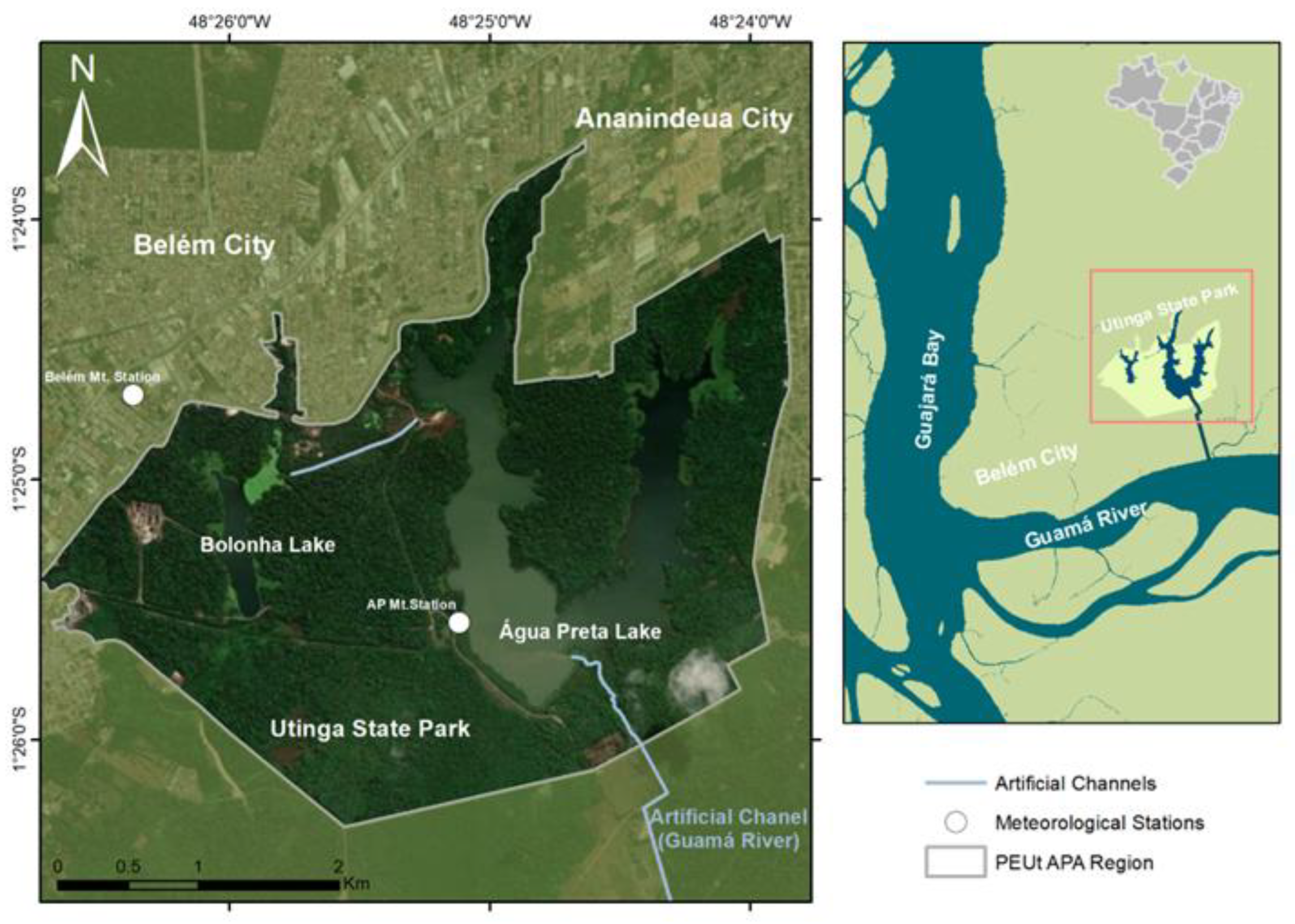
Figure 2.
Meteorological data used in the simulations of Lago Água Preta, including: (A) precipitation and air temperature; (B) wind speed and direction; (C) relative humidity; and (D) solar radiation.
Figure 2.
Meteorological data used in the simulations of Lago Água Preta, including: (A) precipitation and air temperature; (B) wind speed and direction; (C) relative humidity; and (D) solar radiation.
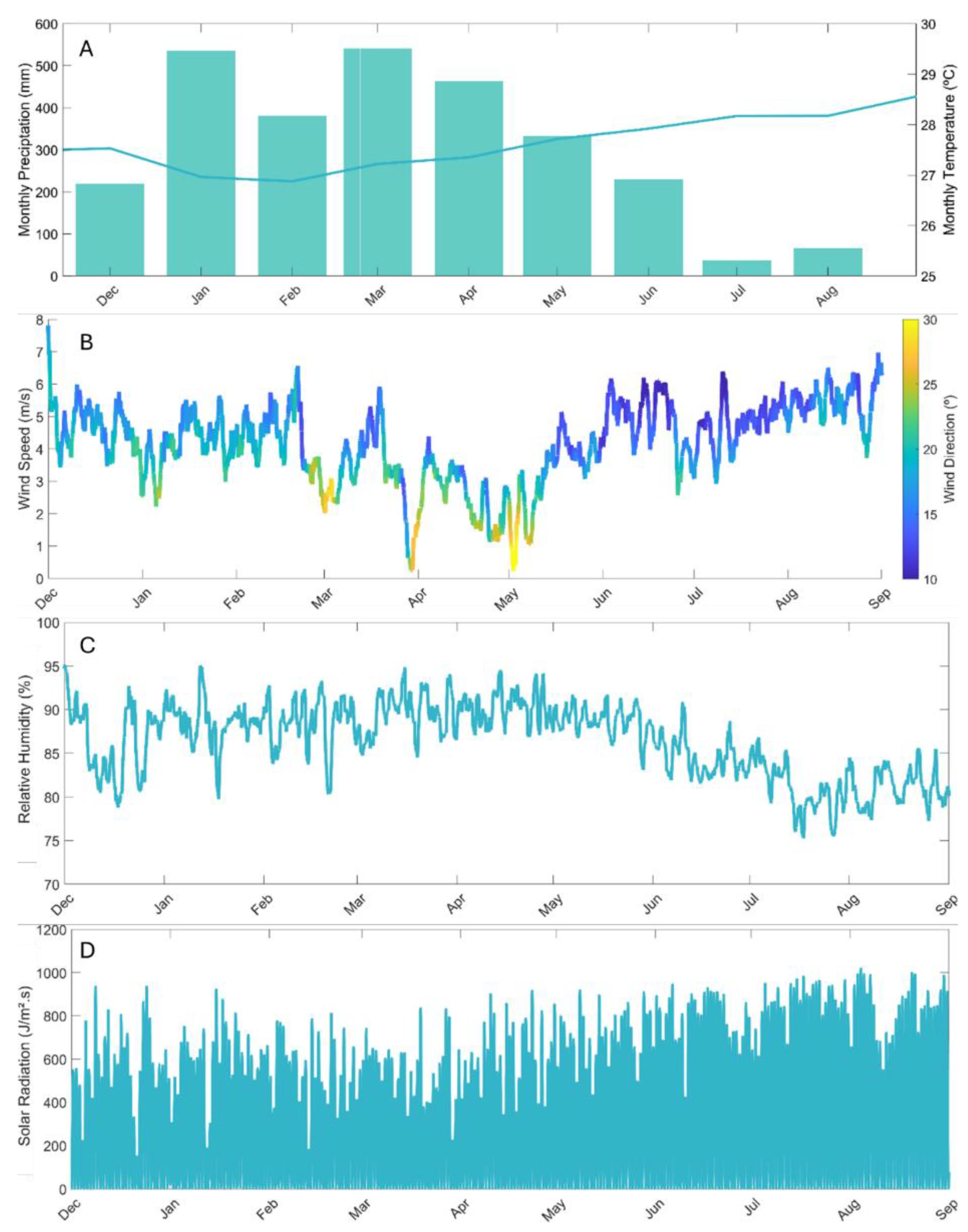
Figure 3.
Illustration of the discretized domain, highlighting the lake's bathymetry, sampling points, and the system’s water inflow and outflow locations.
Figure 3.
Illustration of the discretized domain, highlighting the lake's bathymetry, sampling points, and the system’s water inflow and outflow locations.
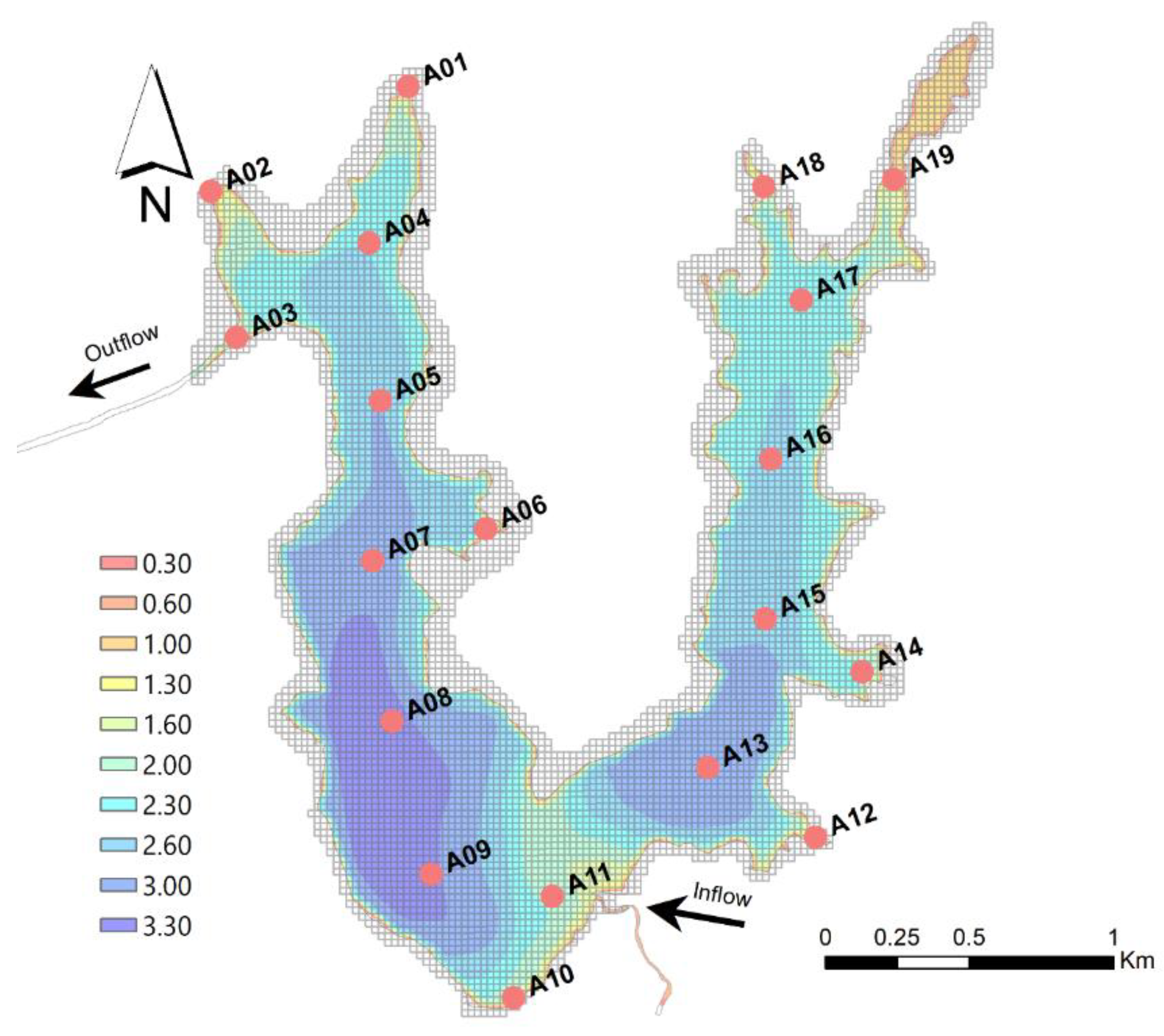
Figure 4.
(a) Comparison between simulated and observed temperature profiles for February. (b) Linear regression between observed and simulated temperature values, showing a strong positive correlation (ρ = 0.89) and a good regression fit (R² = 0.79).
Figure 4.
(a) Comparison between simulated and observed temperature profiles for February. (b) Linear regression between observed and simulated temperature values, showing a strong positive correlation (ρ = 0.89) and a good regression fit (R² = 0.79).
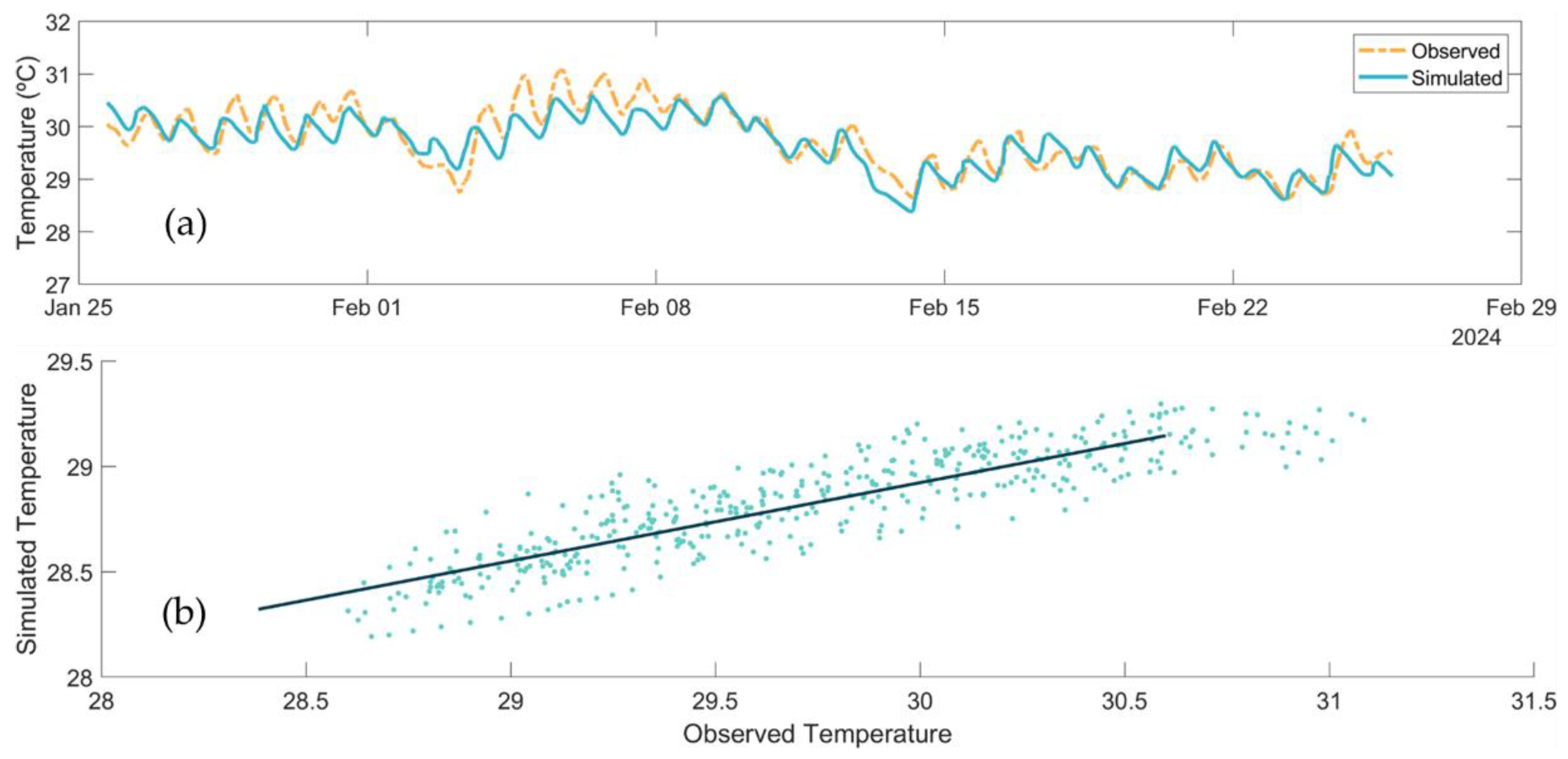
Figure 5.
Variation of current velocity at sampling points A08 and A13, measured 0.5 meters above the lake bed.
Figure 5.
Variation of current velocity at sampling points A08 and A13, measured 0.5 meters above the lake bed.
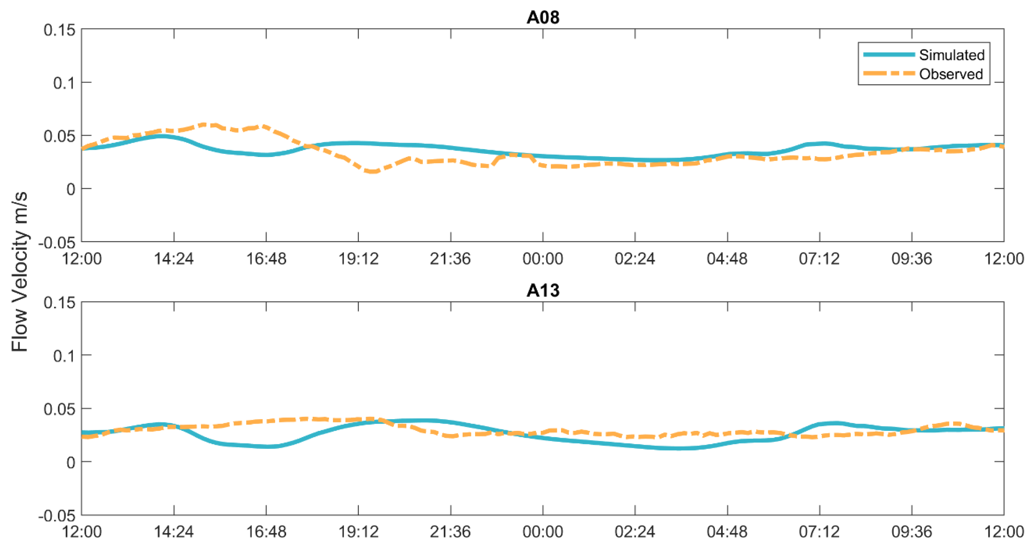
Figure 6.
Água Preta Lake zonation, defined into 3 areas: West, Central, and East. This classification was based on the hydrodynamic characteristics unique to each area.
Figure 6.
Água Preta Lake zonation, defined into 3 areas: West, Central, and East. This classification was based on the hydrodynamic characteristics unique to each area.
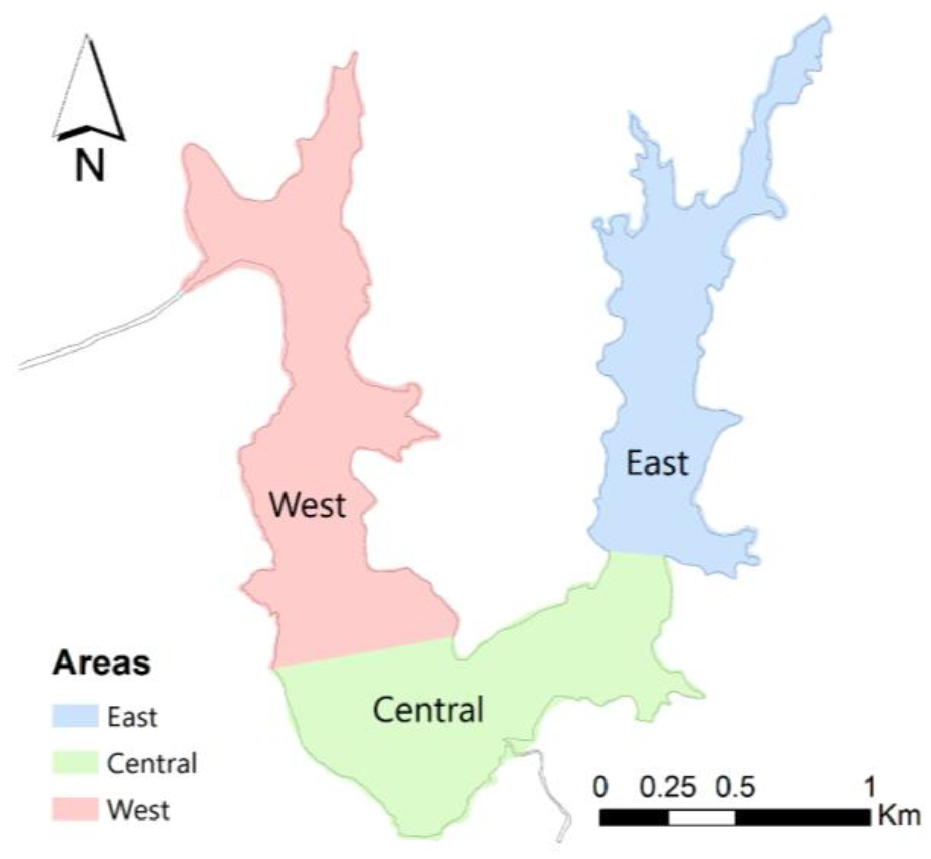
Figure 7.
Average current velocity for February (wet season) and June (dry season), 2024, highlighting the lake’s circulation patterns and maximum velocities associated with the system’s inflow and outflow points.
Figure 7.
Average current velocity for February (wet season) and June (dry season), 2024, highlighting the lake’s circulation patterns and maximum velocities associated with the system’s inflow and outflow points.
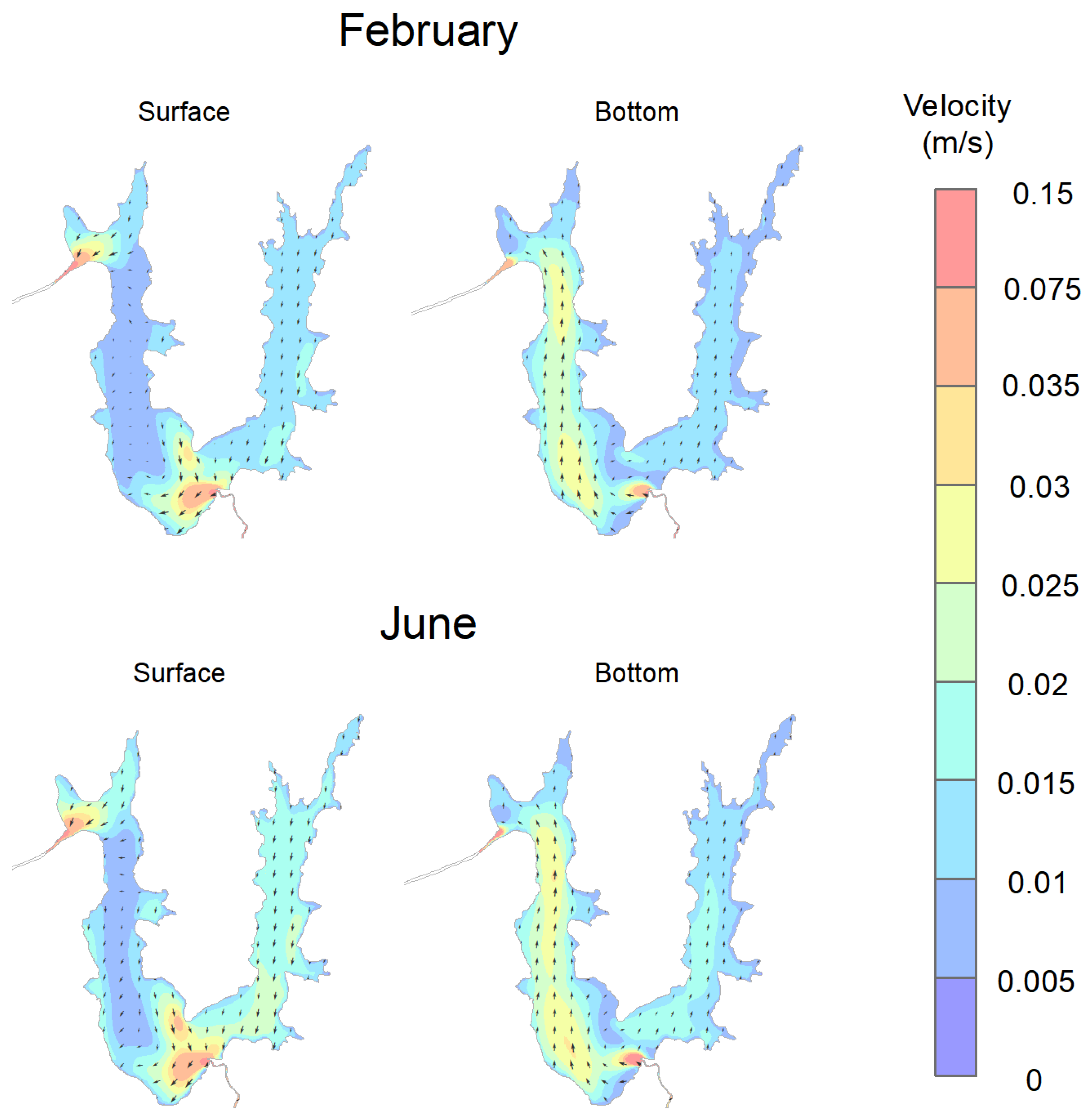
Figure 8.
Temperature variation in February (wet season) and June (dry season) as a function of depth (y-axis) and time (x-axis). The analysis was performed at three representative points—A07 (western zone), A10 (central zone), and A16 (eastern zone)—to better understand the spatial and temporal variability of the lake.
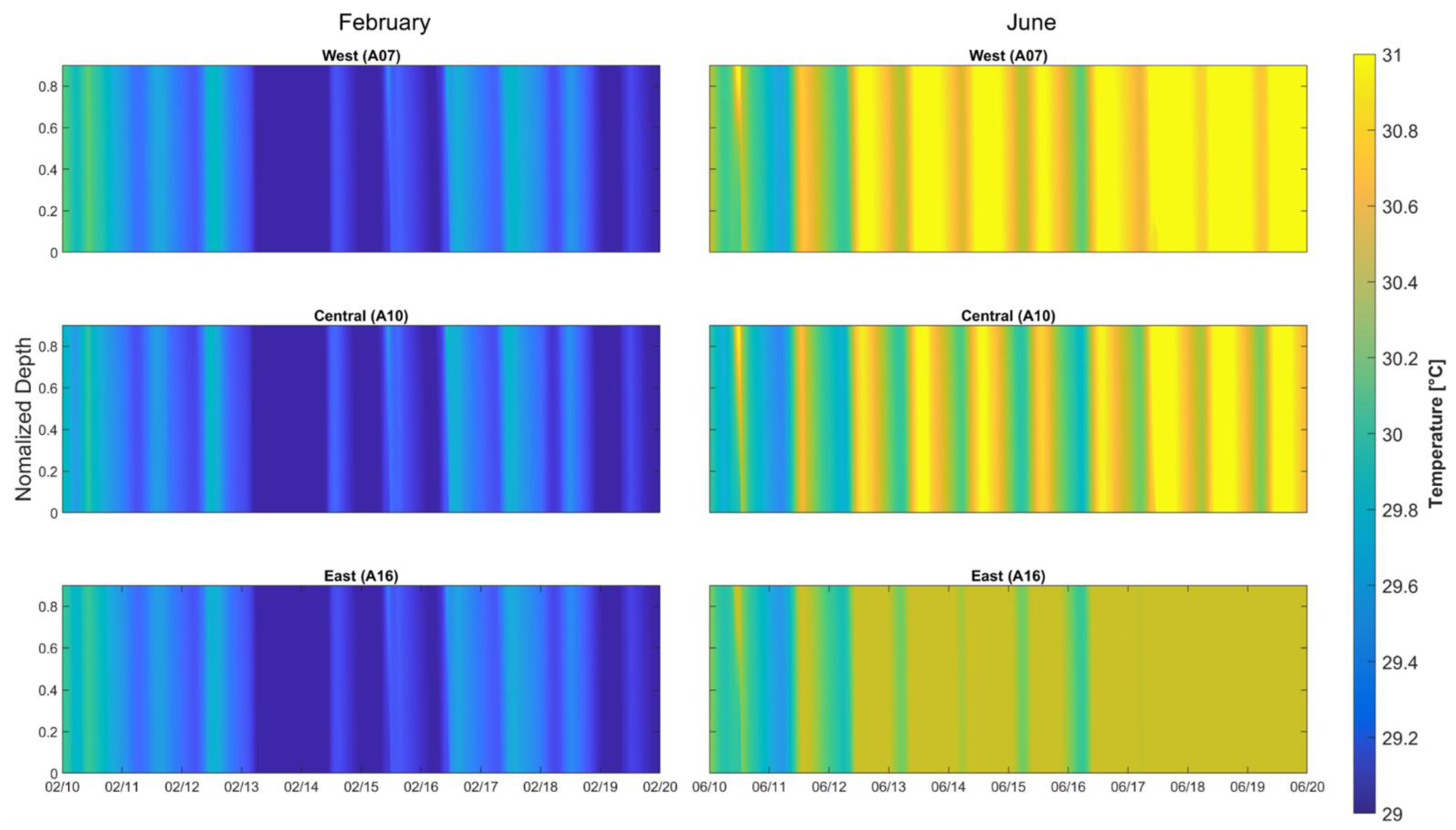
Figure 9.
Horizontal temperature gradient at the surface and at depth, highlighting the differences between the two regional seasonal periods: wet season (February) and dry season (June).
Figure 9.
Horizontal temperature gradient at the surface and at depth, highlighting the differences between the two regional seasonal periods: wet season (February) and dry season (June).
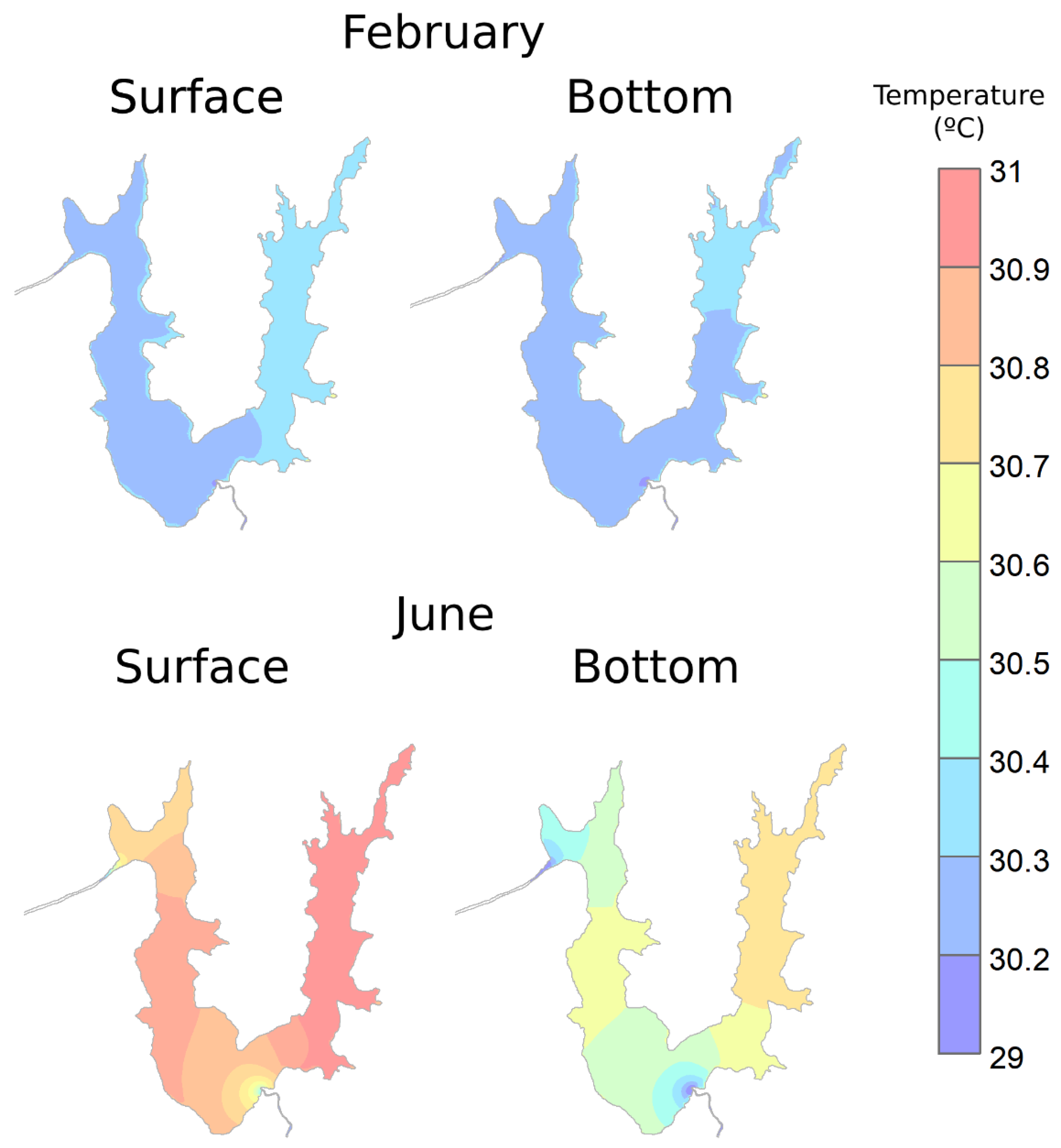
Figure 10.
Suspended sediment transport in m³/s/m, showing that the majority of sediment flows through the central region of the lake due to the influence of the inflow.
Figure 10.
Suspended sediment transport in m³/s/m, showing that the majority of sediment flows through the central region of the lake due to the influence of the inflow.
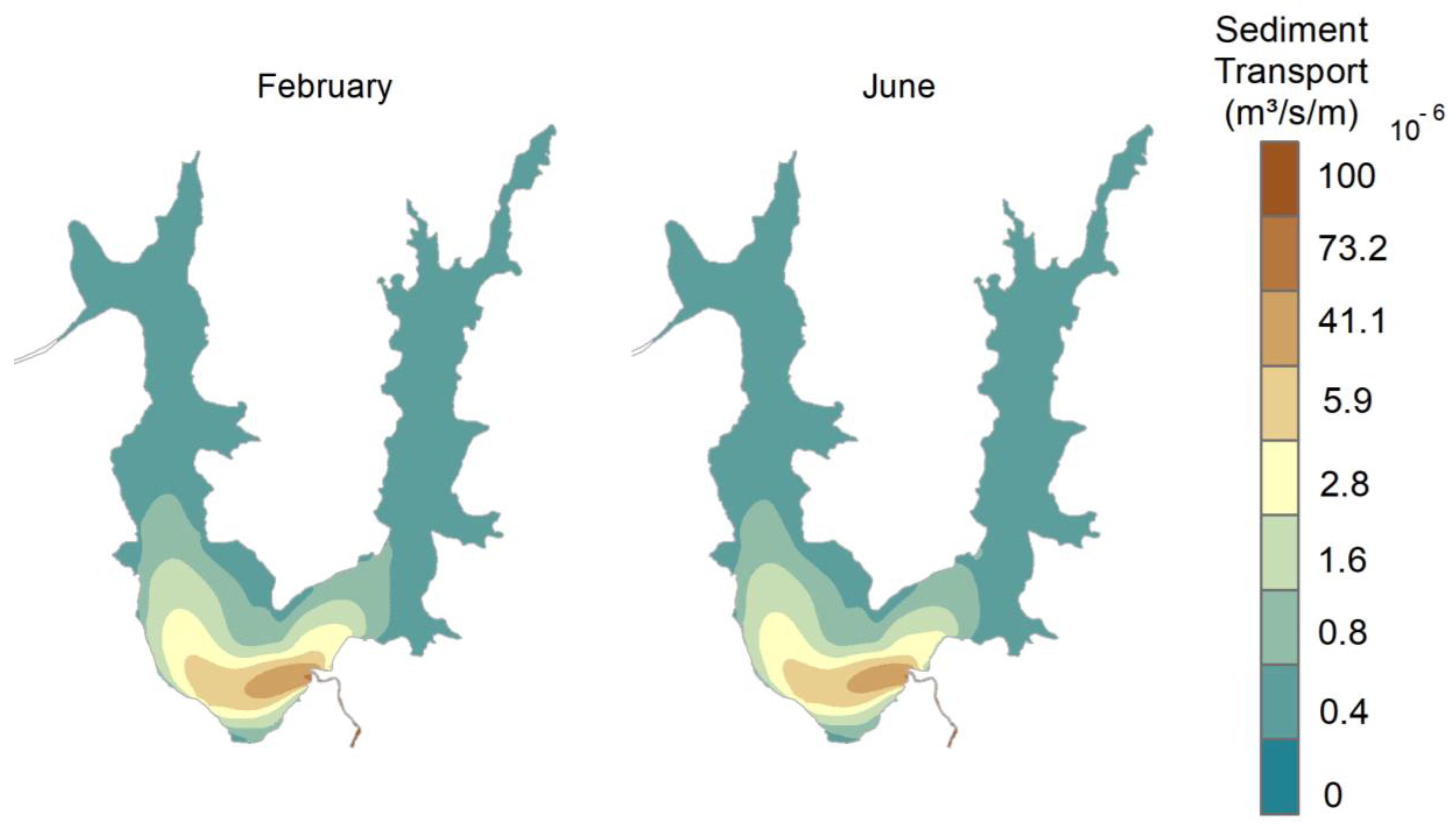

Table 1.
Modified monthly inflow discharge data provided by the Pará State Sanitation Company (COSANPA).
Table 1.
Modified monthly inflow discharge data provided by the Pará State Sanitation Company (COSANPA).
| Months/year | Discharge(m³/s) | Months/year | Discharge(m³/s) |
| nov/23 | 20 | may/24 | 16 |
| dec/23 | 19 | jun/24 | 18 |
| jan/24 | 16 | jul/24 | 19 |
| feb/24 | 14 | aug/24 | 20 |
| mar/24 | 14 | sep/24 | 20 |
| apr/24 | 14 | oct/24 | 19 |
Table 2.
Calculated Manning’s roughness values, classified according to the specific characteristics of each region in the domain.
Table 2.
Calculated Manning’s roughness values, classified according to the specific characteristics of each region in the domain.
| Region | Manning Roughness value |
| Region dominated by macrophytes | 0.030 |
| Sandy sediment predominance region | 0.025 |
| Sandy-silty sediment region | 0.018 |
| Silty sediment region | 0.016 |
Table 3.
Statistical metrics calculated between the simulation and CTD profile data collected at points A01 to A19, highlighting points with higher uncertainties associated with their specific local characteristics: A01, A09, A11, and A17.
Table 3.
Statistical metrics calculated between the simulation and CTD profile data collected at points A01 to A19, highlighting points with higher uncertainties associated with their specific local characteristics: A01, A09, A11, and A17.
| R | RMSE (ºC) | R² | MAE (ºC) | |||||||||||||
| Pts | Dec | Feb | Jun | Aug | Dec | Feb | Jun | Aug | Dec | Feb | Jun | Aug | Dec | Feb | Jun | Aug |
| A01* | -0.05* | 0.85 | 0.82 | 0.96 | 0.78 | 0.78 | 0.87 | 0.34 | 0.00 | 0.72 | 0.68 | 0.91 | 0.98 | 1.31 | 1.16 | 0.39 |
| A02 | 0.95 | 0.85 | 0.94 | 0.83 | 0.80 | 0.26 | 0.42 | 0.26 | 0.91 | 0.74 | 0.89 | 0.69 | 0.91 | 0.43 | 0.64 | 0.28 |
| A03 | -0.29 | 0.86 | 0.99 | 0.96 | 0.24 | 0.41 | 0.57 | 0.37 | 0.08 | 0.73 | 0.99 | 0.91 | 0.27 | 0.70 | 0.75 | 0.50 |
| A04 | 0.91 | 0.79 | 0.41 | 0.36 | 0.25 | 0.39 | 0.69 | 0.41 | 0.83 | 0.63 | 0.17 | 0.13 | 0.33 | 0.51 | 1.19 | 0.45 |
| A05 | 0.98 | 0.86 | 0.97 | 0.47 | 0.24 | 0.46 | 0.43 | 0.25 | 0.96 | 0.74 | 0.94 | 0.22 | 0.29 | 0.49 | 0.69 | 0.35 |
| A06 | 0.92 | 0.86 | 0.86 | 0.69 | 0.40 | 0.41 | 0.62 | 0.51 | 0.84 | 0.74 | 0.74 | 0.48 | 0.56 | 0.46 | 0.97 | 0.63 |
| A07 | 0.90 | 0.91 | 0.84 | 0.89 | 0.38 | 0.60 | 0.50 | 0.55 | 0.82 | 0.82 | 0.70 | 0.80 | 0.47 | 0.72 | 0.97 | 0.91 |
| A08 | 0.95 | 0.96 | 0.86 | 0.91 | 0.55 | 0.66 | 0.39 | 0.47 | 0.90 | 0.91 | 0.74 | 0.83 | 0.65 | 0.71 | 0.69 | 0.62 |
| A09* | 0.73 | 0.69 | 0.97 | -0.30* | 0.52 | 0.75 | 0.19 | 0.32 | 0.53 | 0.48 | 0.93 | 0.09 | 0.56 | 0.91 | 0.30 | 0.41 |
| A10 | 0.97 | 0.99 | 1.00 | 0.93 | 0.37 | 0.63 | 0.59 | 0.46 | 0.93 | 0.97 | 0.99 | 0.86 | 0.48 | 0.68 | 0.82 | 0.75 |
| A11* | 0.95 | 0.31 | -0.65* | 0.94 | 0.50 | 0.52 | 0.08 | 0.56 | 0.90 | 0.10 | 0.42 | 0.89 | 0.62 | 0.68 | 0.12 | 0.72 |
| A12 | 0.94 | 0.99 | 0.94 | 0.86 | 0.25 | 0.81 | 0.26 | 0.18 | 0.87 | 0.98 | 0.88 | 0.73 | 0.38 | 0.87 | 0.43 | 0.24 |
| A13 | 0.94 | 0.95 | 0.91 | 0.98 | 0.35 | 0.67 | 0.40 | 0.14 | 0.88 | 0.90 | 0.82 | 0.95 | 0.72 | 0.75 | 0.60 | 0.24 |
| A14 | 0.84 | 0.88 | 0.80 | 0.98 | 0.21 | 0.50 | 0.30 | 0.48 | 0.70 | 0.77 | 0.63 | 0.97 | 0.34 | 0.71 | 0.56 | 0.72 |
| A15 | 0.98 | 0.87 | 0.92 | 0.67 | 0.35 | 0.51 | 0.44 | 0.29 | 0.96 | 0.76 | 0.84 | 0.45 | 0.64 | 0.61 | 0.65 | 0.50 |
| A16 | 0.87 | 0.88 | 0.88 | 0.90 | 0.43 | 0.57 | 0.49 | 0.31 | 0.75 | 0.78 | 0.77 | 0.82 | 0.68 | 0.94 | 0.73 | 0.53 |
| A17* | 0.99 | 0.92 | -0.19* | 0.95 | 0.18 | 0.10 | 0.87 | 0.56 | 0.97 | 0.85 | 0.04 | 0.90 | 0.33 | 0.18 | 2.04 | 0.83 |
| A18 | 0.96 | 0.55 | 0.89 | 0.89 | 0.56 | 0.77 | 0.44 | 0.20 | 0.93 | 0.30 | 0.80 | 0.80 | 0.96 | 1.40 | 0.63 | 0.41 |
| A19 | 0.56 | 0.65 | 0.99 | 0.98 | 0.74 | 0.62 | 0.53 | 0.93 | 0.32 | 0.42 | 0.97 | 0.96 | 1.07 | 1.16 | 0.60 | 1.34 |
* Values with low statistical metrics due to specific local conditions affecting these observation points.
Disclaimer/Publisher’s Note: The statements, opinions and data contained in all publications are solely those of the individual author(s) and contributor(s) and not of MDPI and/or the editor(s). MDPI and/or the editor(s) disclaim responsibility for any injury to people or property resulting from any ideas, methods, instructions or products referred to in the content. |
© 2025 by the authors. Licensee MDPI, Basel, Switzerland. This article is an open access article distributed under the terms and conditions of the Creative Commons Attribution (CC BY) license (http://creativecommons.org/licenses/by/4.0/).
Copyright: This open access article is published under a Creative Commons CC BY 4.0 license, which permit the free download, distribution, and reuse, provided that the author and preprint are cited in any reuse.


