Submitted:
03 July 2025
Posted:
04 July 2025
You are already at the latest version
Abstract
Options hedging in real-world markets is challenged by strong asset correlations, partial observability, and nonstationary price dynamics. These conditions limit the effectiveness of traditional strategies and pose challenges for reinforcement learning (RL) methods, which often overfit or become unstable in high-dimensional environments. Existing RL hedging methods suffer from static risk measures and inflexible policies, leading to issues in stability, adaptability, and generalization. To address these challenges, we propose Deep Diffusion Reinforcement Learning (DDRL), a new RL framework that integrates the Soft Actor-Critic (SAC) algorithm with diffusion-based generative policy networks for dynamic hedging. By modeling policy distributions through a denoising diffusion process, DDRL effectively captures nonlinear dependencies and generates more robust actions. To improve stability, DDRL also incorporates double critic networks, entropy regularization, soft target updates, and other technical enhancements. We implement DDRL in a simulated trading environment based on historical market data. Empirical results show that DDRL reduces hedging losses and transaction costs compared to baseline RL methods, while maintaining stable performance across varied portfolio configurations and market conditions. These results highlight the potential of generative diffusion policies to enhance the robustness and reliability of RL-based financial decision-making.
Keywords:
diffusion model
; options hedging
; reinforcement learning
1. Introduction
Options hedging serves as a crucial tool in modern financial risk management, playing a significant role in mitigating potential portfolio losses and improving capital efficiency [1,2,3,4]. For instance, a corn producer may purchase put options to lock in a minimum selling price, thereby hedging against potential price declines. Traditional financial theories, such as the Black-Scholes (BS) model and the Black–Scholes–Merton (BSM) model, have laid the theoretical foundations for options hedging [5,6]. However, these models are based on idealized assumptions, including log-normal asset returns, constant volatility, and frictionless markets. These assumptions are often unrealistic in real markets, limiting the models’ practical effectiveness.
To address model uncertainty, market non-stationarity, and transaction frictions, researchers have increasingly turned to dynamic hedging approaches. Marzban et al. [7] employed dynamic programming (DP), which derives optimal strategies through value or policy iteration under a known market model, and is well-suited for handling time-dependent state transitions. However, this method suffers from two major limitations: first, DP relies on accurate modeling of market dynamics, which is often unavailable in practice; second, DP is subject to the "curse of dimensionality", making it computationally infeasible in high-dimensional state spaces [7].
To overcome these challenges, reinforcement learning (RL) has recently emerged as a leading solution for high-dimensional, model-free optimization problems [8,9,10,11,12,13,14,15]. Unlike traditional approaches, RL does not rely on prior market modeling, instead, it learns optimal strategies by interacting with the environment and optimizing a reward function [9]. Buehler et al. [8] were among the first to formulate the options hedging problem within a RL framework, using convex risk measures to evaluate terminal wealth and laying the foundation for RL applications in derivative risk management. Subsequent studies [10,11] have explored various risk objectives and advanced the application of RL in over-the-counter (OTC) options hedging. Nonetheless, several key limitations remain.
First, existing RL methods predominantly rely on static risk measures [12,13,14,15], lacking the ability to model the dynamic evolution of risk. This leads to severe time-inconsistency issues, wherein pre-planned hedging strategies may become invalid under changing market conditions. Second, from an algorithmic perspective, most RL methods adopt either actor-only or critic-only optimization schemes [12,16], which tend to overestimate value functions and degrade training stability [17]. These methods typically rely on an assumed equivalence to DP structures—an assumption that breaks down when static risk measures are employed [18]. Moreover, to enhance strategy generalization, researchers have increasingly incorporated high-dimensional state representations, such as Greeks and the implied volatility [19,20]. This, however, introduces new challenges, including sample sparsity and training instability in financial environments where data acquisition is costly and limited. As the state space increases, most RL methods using multi-layer perceptrons (MLPs) as policy networks suffer from limited expressive power due to their linear assumptions, making them prone to overfitting and unable to capture complex nonlinear relationships, which in turn affects the model’s generalization and stability [21]. Even advanced continuous control algorithms such as Deep Deterministic Policy Gradient (DDPG) [22] and Soft Actor-Critic (SAC) [23] exhibit instability and convergence issues in volatile and feature-rich financial environments [17].
To overcome these limitations, we propose a novel hedging framework—Deep Diffusion Reinforcement Learning (DDRL). Our approach offers key innovations in the following areas: (1) Improved time consistency and policy implementability: DDRL supports continuous action selection and employs a step-wise reward function dynamically defined by profit-and-loss and trading costs. Combined with the sequential modeling ability of diffusion models, this improves temporal consistency and makes the learned policies more implementable in real markets. (2) Enhanced training stability and policy performance: By incorporating a dual-critic structure, entropy regularization and soft target updates, DDRL mitigates value overestimation and policy instability, leading to more stable training and more precise policy optimization. (3) Handling high-dimensional state spaces: The policy network in DDRL adopts a diffusion-based generative architecture that captures complex nonlinear dependencies without relying on structural priors, thereby enhancing both generalization and expressiveness—an essential contribution to financial RL.
To enhance realism, DDRL is trained under a stochastic volatility environment modeled by the SABR framework, incorporating transaction costs and market frictions. Extensive experiments demonstrate the superior performance of DDRL across different market conditions. Compared to baseline RL methods, DDRL reduces potential maximum loss by up to 37.93% and transaction costs by up to 31.53%, showing strong robustness and adaptability in complex financial markets. Overall, we may summarize the contributions of this paper as follows:
- We propose DDRL, the first RL framework for options hedging that incorporates diffusion models as policy networks. To the best of our knowledge, this is the first attempt to combine diffusion models with RL for financial decision-making tasks.
- By dynamically incorporating step-wise profit-and-loss and trading costs into the reward, DDRL captures market frictions and avoids static risk assumptions, enabling consistent and adaptive hedging decisions over time.
- DDRL employs a dual-critic architecture with entropy regularization to enhance training stability, effectively addressing value overestimation and premature convergence in volatile hedging environments.
- We validate DDRL under realistic SABR-simulated market conditions, showing substantial improvements in hedging effectiveness in terms of cost efficiency, risk reduction, and policy robustness.
The remainder of this paper is organized as follows: Section 2 provides a review of related work on options hedging using traditional methods and RL, and generative diffusion models applied to optimization. Section 3 presents the algorithm implementation. Section 4 introduces experiments. Section 5 presents the experimental results and Section 6 concludes the paper with a discussion of findings and potential future research directions.
2. Related Work
2.1. Traditional Options Hedging Methods
The Black-Scholes (BS) model [5] has long been a fundamental tool for pricing options and developing hedging strategies. It assumes that asset prices follow a log-normal distribution with constant volatility, providing critical sensitivities such as Delta, Gamma, and Vega [6], which are essential for hedging. However, in real-world markets, the BS model has notable limitations. It doesn’t account for volatility changes or other irregular market behaviors [24], and its static nature makes it ill-suited to the dynamic nature of markets [19,25]. Moreover, the model is built on the idealized assumption of frictionless markets, ignoring the inevitable transaction costs and slippage present in real-world trading. Traditional BS-based strategies often focus on a single risk factor and fail to capture the interactions between multiple factors, limiting their effectiveness in complex market environments.
2.2. RL for Dynamic Hedging
Table 1 provides a systematic summary of recent RL methods for option hedging and their core characteristics, highlighting a clear evolution from early theoretical validation to adaptation in complex real-world environments. This development can be analyzed from three key dimensions: algorithm architecture, reward design, and data foundation.
In terms of algorithm architecture, early studies primarily employed value-based methods (such as Q-Learning and SARSA) for discrete action spaces [26,27], but their limited action sets made it difficult to precisely adjust portfolios, resulting in poor generalization performance. Subsequently, policy gradient and actor-critic architectures (e.g., DDPG, TD3, D4PG) [15,19,30] improved learning capabilities in continuous environments, with PPO becoming widely used due to its favorable convergence and stability properties [28]. However, most methods still rely on MLPs, which struggle to capture nonlinear relationships in financial markets, especially in high-dimensional spaces, where gradient explosion is common [21]. Additionally, the sparsity of financial data can lead to overfitting, and traditional RL methods perform poorly in handling long-term dependencies, affecting their performance in real market conditions [37].
In terms of reward function design, early research often used simple objective functions such as or its penalized form [28,32]. While easy to implement, these methods overlook risk factors and fail to capture the risk-return trade-off inherent in financial markets. To address this, later studies introduced risk-aware objectives such as mean-variance and CVaR [13,19], and incorporated transaction costs and tail risk into the reward function to enhance practical applicability. However, most methods still rely on static risk measures, which struggle to handle dynamic market changes and may lead to time inconsistency issues.
In terms of data foundation, early methods primarily used synthetic data generated from the Black-Scholes model with GBM [26,28]. While these data are useful for validating algorithm convergence, they deviate significantly from real market behavior, limiting the model’s generalizability. In recent years, researchers have shifted to using more complex synthetic environments, such as the SABR and Heston models, and GAN-based simulators [13,30], to better replicate the statistical characteristics of financial markets. These approaches have improved the representativeness and complexity of the simulated data. Additionally, some studies have started testing on real market data, such as S&P and DJIA indices [33,34], to improve practical applicability.
Compared to the methods above, our proposed DDRL excels in time consistency, stability, and handling high-dimensional nonlinear structures, making it particularly well-suited for volatile, cost-sensitive financial environments.
2.3. Diffusion Models in Optimization and RL
Diffusion models, originally developed for generative tasks such as image synthesis [38] and molecular design [39], have recently emerged as a novel tool in the domain of optimization and RL. These models simulate a stochastic diffusion process in latent space, enabling the modeling of complex, high-dimensional, and multimodal distributions that are often encountered in real-world decision-making tasks. While early applications were largely limited to offline settings, such as Diffusion Q-Learning (DQL) [40] for behavior cloning, recent studies have begun to explore their potential in broader RL contexts. For example, Du et al. [41] demonstrated that diffusion-based policies can outperform traditional RL algorithms like PPO and SAC in utility maximization tasks, highlighting their ability to navigate intricate objective landscapes. Despite recent progress, applying diffusion models in RL remains a relatively new area, with few studies addressing their use in continuous control tasks within financial settings. In this paper, we leverage the strong modeling capabilities of diffusion models to propose an options hedging strategy optimized for continuous action spaces, further enhancing the robustness and adaptability of the strategy. This represents a meaningful step forward in applying generative models to financial decision-making tasks.
3. Deep Diffusion Reinforcement Learning for Options Hedging
3.1. RL Formulation
We formulate the options hedging problem as a sequential decision-making task under uncertainty, modeled as a Markov Decision Process (MDP) defined by the tuple , where:
- denotes the state space;
- is the action space;
- is the transition kernel that governs state dynamics;
- is the reward function;
- is the discount factor.
The agent interacts with the environment by selecting actions according to a policy , with the goal of maximizing expected cumulative rewards. Formally, the action-value function under policy is:
where denotes the trajectory distribution induced by , and K is the time horizon. The optimal policy satisfies:
This setup enables the use of high-capacity RL algorithms—particularly those suited to continuous control and high-dimensional state spaces, such as Soft Actor-Critic (SAC) and Proximal Policy Optimization (PPO).
3.2. RL Design
An overview of our RL framework, highlighting the custom-designed state, action, and reward components, is shown in Figure 1. Each component is described in detail below.
3.2.1. State Representation
At each decision point , the agent observes a seven-dimensional state vector:
where is the underlying asset price, and the Greek symbols represent sensitivities (Delta, Gamma, Vega) for both the overall portfolio and a designated ATM option.This feature set captures key aspects of market and portfolio risk exposures, allowing the agent to adapt to dynamic risk profiles. Compared to conventional low-dimensional summaries [26,27], this representation supports richer decision-making, albeit at the cost of increased learning complexity.
3.2.2. Action Space and Hedging Constraints
The action specifies the proportion of ATM options to engage for hedging. The actual hedge volume is given by , with the following constraints enforced to maintain stable risk exposures:
These bounds prevent over-hedging and ensure that net exposures remain within a controlled amplification of the original risk, thereby promoting effective yet conservative risk management.
3.2.3. Reward Design
The reward function balances trading costs against portfolio performance. At each step i, the reward is defined as:
where denotes the per-unit transaction cost, is the prevailing market value of the ATM option, and is the total mark-to-market value of the hedged portfolio. This design encourages cost-aware, value-enhancing decisions. Unlike static terminal risk objectives such as CVaR, which often induce myopic or unstable behavior, our reward provides time-consistent incentives for incremental risk reduction. This dynamic structure promotes hedging discipline and aligns with long-horizon risk-neutral mandates in institutional settings.
4. Algorithm Architecture
The algorithm architecture of DDRL, as shown in Figure 2 and Algorithm 1, consists of several components that work together to optimize the policy.
| Algorithm 1:DDRL: Deep Diffusion Reinforcement Learning |
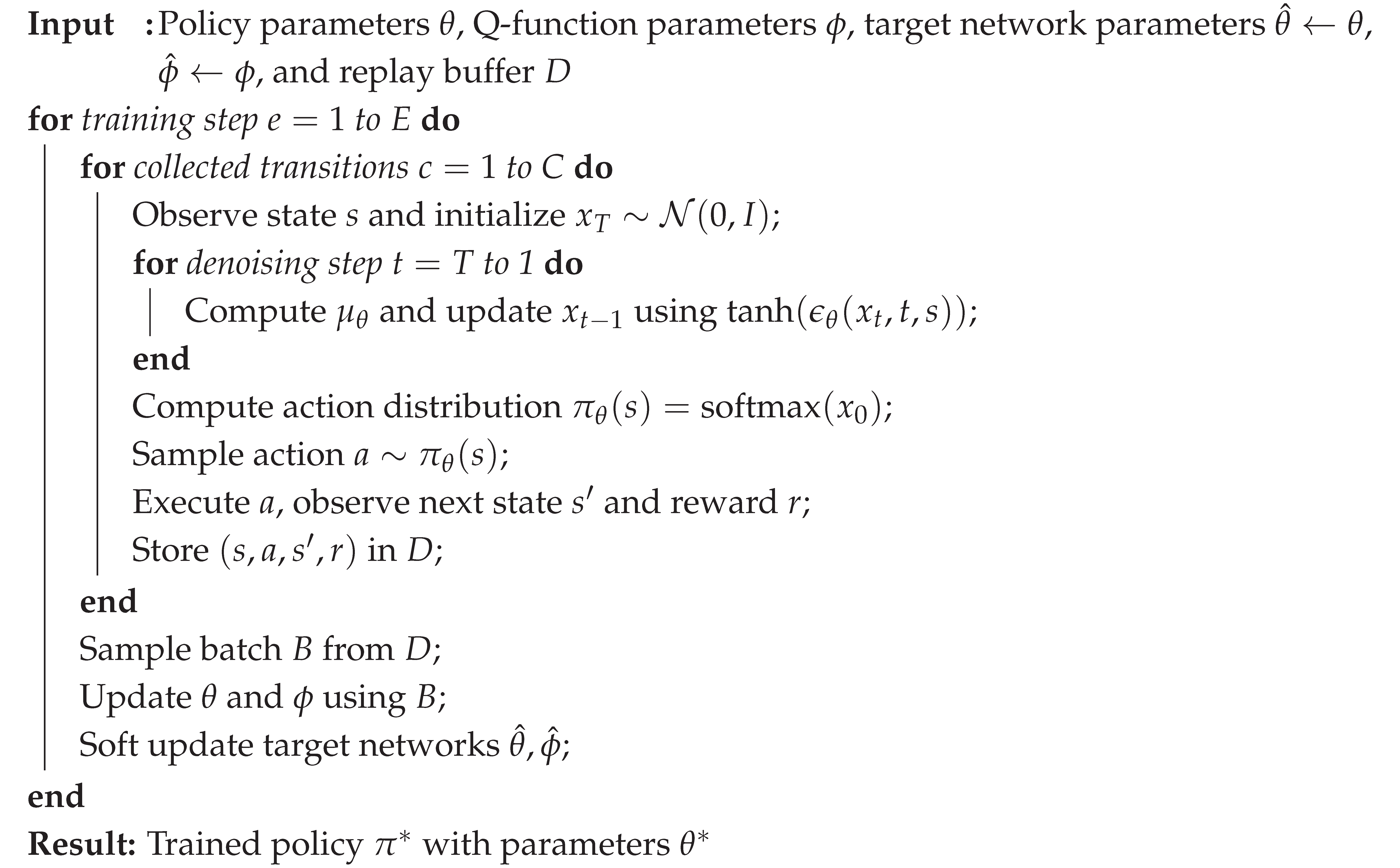 |
4.1. Diffusion-Based Policy Network (DPN)
At the heart of DDRL lies a Diffusion-Based Policy Network (DPN), which replaces the conventional actor network to enhance stability, expressiveness, and robustness in high-dimensional, multi-modal action spaces. DPN generates actions by modeling the action-sampling process as a reverse diffusion procedure. Starting from a latent Gaussian variable , the model performs iterative denoising:
where is the latent variable at diffusion step t, and is the denoising network conditioned on state . The scalars , , and follow a fixed or learned noise schedule over T denoising steps.
After T steps of reverse denoising, the final latent is mapped to action logits:
where W and b are learnable affine parameters. This generative design enables the policy to represent complex, stochastic behaviors and mitigates the mode collapse often seen in deterministic actors.
To train the DPN, a denoising loss is jointly optimized alongside the reinforcement objective:
where is sampled from a known forward diffusion distribution. This loss encourages to approximate the true noise and improves sample quality and diversity.
4.2. Trajectory Collection and Experience Replay
DDRL interacts with the environment using the generative policy , where each action is sampled via the denoising process described above. Collected transitions are stored in a replay buffer .
In domains with delayed or episodic rewards, immediate rewards may not be available at each step. Instead, they are computed retrospectively based on trajectory-level outcomes such as final profit-and-loss (PnL) or risk sensitivities (e.g., delta, gamma). These rewards are filled in post-hoc after trajectory termination. This hybrid trajectory-level processing, combined with standard experience replay, improves sample efficiency and supports learning under complex reward structures.
4.3. Policy Optimization with Entropy Regularization
To encourage exploration and avoid premature convergence, DDRL adopts the maximum entropy RL paradigm. The overall policy objective is:
where is a tunable entropy temperature. Importantly, since DPN is a generative model, actions are obtained via the reparameterization trick: , where is deterministically computed from noise and state .
This allows gradients to backpropagate through the diffusion sampling process:
This formulation enables stable end-to-end training of the denoising policy network via stochastic gradient descent.
4.4. Critic Learning and Target Value Estimation
DDRL employs a double Q-network architecture to mitigate overestimation bias in value targets. The critic networks and are trained by minimizing the Bellman residual:
with the target value computed as:
Here, is sampled via the same DPN-based reverse diffusion mechanism to maintain consistency in target evaluation. To reduce value estimate oscillations, the target networks are updated via Polyak averaging:
This structure ensures stable critic updates and coherent interaction between the generative actor and evaluative critics.
5. Experiment
5.1. Datasets Simulation
We generated key data required for options pricing and hedging strategies using the SABR model [42] and the BSM formula [5]. This data includes the underlying asset price, volatility, implied volatility, option prices, and various Greek letters, all of which are crucial for formulating and evaluating financial hedging strategies.
The SABR model, in particular, offers the advantage of more accurately and comprehensively reflecting the volatility surface, making it an essential tool for options traders and risk managers. The risk-neutral behavior of the underlying asset price S and its volatility is governed by the following stochastic processes:
In this model, and represent Wiener processes that share a constant correlation . The parameters v (volatility of volatility), r (risk-free rate), and q (dividend yield) are assumed to be constant. Additionally, we consider the real-world expected return to be constant. The asset price process in the real-world follows the same form as the previously mentioned equation, but with replaced by .
The initial values and correspond to the starting values of and S, respectively. For a European call options with strike price K and time to maturity T, the implied volatility is estimated as when , or in other cases.
represents the risk-neutral present value of the future asset price, while B and serve as correction factors. quantifies the normalized effect of price changes on volatility.
With the implied volatility , the option’s value can be calculated using the Black-Scholes-Merton formula as follows:
where
here, N denotes the cumulative normal distribution function. When , the implied volatility remains constant at , reducing the SABR model to the BSM options pricing model [5].
As discussed, Delta is the first derivative of the options price with respect to the asset price, Gamma is the second derivative, and Vega is the first derivative with respect to volatility. In theory, the price of a European option can be treated as a function of the underlying asset price S and volatility for the purpose of calculating these derivatives. However, in practice, the option price is typically treated as a function of the underlying asset price S and the implied volatility when calculating the Greek letters. We will follow this approach. Delta, Gamma, and Vega, denoted as , , and , are derived as follows:
The Delta, Gamma, and Vega of a portfolio are calculated by summing those for the individual options in the portfolio.The dividend yield q affects the arbitrage-free price path of the asset. In the formula, the term is used to discount the future price of the asset, accounting for the impact of dividend payments on the asset price.
5.2. Baselines
In our experiments, we compared the use of delta hedging, delta-gamma hedging, and more advanced RL combined with quantile-based methods as benchmarks. The first two are traditional hedging methods, while the latter is RL method.
- Delta Hedging: Calculated by continuously adjusting the portfolio’s position to ensure that the Delta, or the sensitivity to small price changes in the underlying asset, is neutralized. The goal is to offset price movements by buying or selling the underlying asset.
- Delta-Gamma Hedging: This method adjusts both Delta and Gamma, meaning it neutralizes both the portfolio’s sensitivity to price changes (Delta) and the sensitivity of Delta itself (Gamma). This requires using additional options, making the process more complex but effective in reducing non-linear risk.
- RL: This baseline model is an effective RL method based on the [19], incorporating quantile regression to more accurately predict the distribution of losses and returns.
5.3. Evaluation Metrics
We conducted the hedging experiment with three different objective functions. The objective functions are calculated from the total loss during the 30-day period considered.
The first objective function, Mean-Std, seeks to minimize both the expected loss (mean m) and the uncertainty of the loss (standard deviation s). Under the assumption of a normal distribution, can approximate the 95th percentile of the loss distribution.
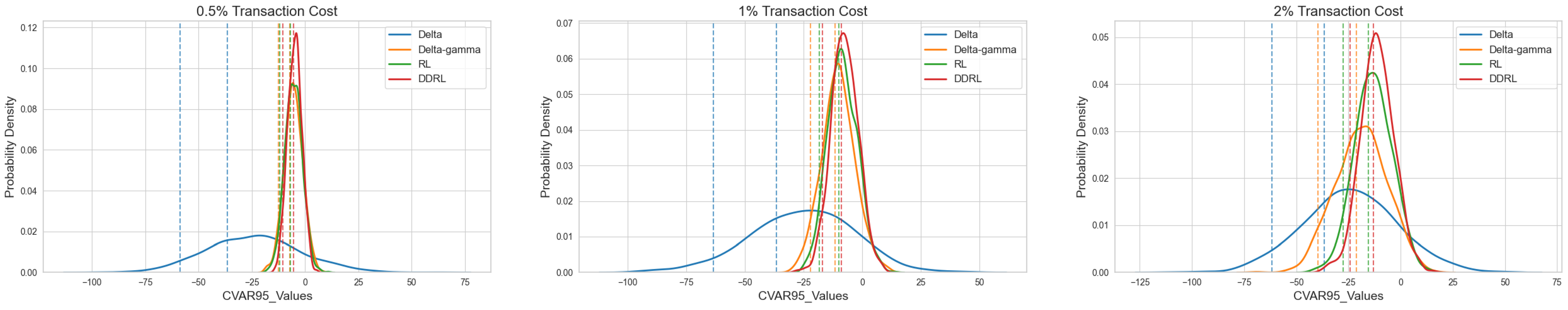
The second and third objective functions minimize VaR and CVaR, both using a 95% confidence level. VaR represents the maximum potential loss at a specific confidence level, with VaR95 indicating the 95th percentile of portfolio loss. On the other hand, CVaR refers to the average loss when losses exceed the VaR threshold, and CVaR95 specifically represents the expected loss in the worst 5% of cases, focusing more on extreme risks and providing further insight into tail risk.
The Gamma Hedge Ratio(R) measures the reduction in gamma exposure after hedging, calculated as:
where and represent the portfolio’s gamma exposure before and after hedging at time t. A ratio closer to 1 indicates more effective gamma hedging.
The Improvement Ratio (IR) in gamma hedging between DDRL and RL is calculated as:
where the ratio refers to their respective Gamma Hedge Ratios.
The Transaction Cost Reduction Ratio (TCR) compares DDRL and RL in terms of transaction costs, calculated as:
where the cost refers to their respective transaction cost.
5.4. Experimental Settings
All experiments were performed on a high-performance workstation (i9-12900K, 64G, RTX 3090). DDRL uses a diffusion model-based actor network and two critic networks with identical structures for evaluation. The actor network predicts the denoised distribution from a random normal distribution and the current state, incorporating sinusoidal positional embeddings [43] to capture temporal information. This helps the network understand the steps in the diffusion process. The actor network has three fully connected layers with Mish activation, except the last layer, which uses Tanh for output normalization. The critic networks share this structure but output Q-values directly without activation. Both networks are trained using the Adam optimizer [44], with learning rates for the actor and for the critic, and a weight decay of for regularization. The target networks have the same structure as the online networks, with a soft update rate of .
As shown in Table 2, we assume the RL agent hedges client orders that arrive following a Poisson process with a daily intensity of 1.0. Each order is for a 60-day option on 100 units of the underlying asset, with an equal chance of being long or short. Experiments are conducted under transaction cost assumptions of 0.5%, 1%, and 2% of the option price. A 30-day ATM option is used for hedging. The initial stock price is set at 10 dollar, and the volatility is 30% annually. We report the results of over 5,000 test scenarios for an average 30-day hedging period. The training simulation consists of 50,000 iterations, and the evaluation simulation consists of 10,000 iterations.These test scenarios are different from the (much larger number of) scenarios used to train the agents. Within each set of tests, the scenarios were kept the same.
5.5. Hedging Results
Table 3 presents the performance comparison of four hedging strategies—Delta, Delta-Gamma, RL, and our proposed DDRL—under constant volatility and varying transaction cost settings (0.5%, 1%, and 2%). The table reports objective values across three risk measures (Mean-Std, VaR95, and CVaR95), as well as supplementary metrics that reflect hedge quality and cost efficiency: Gamma Hedge Ratio, IR, and TCR.
- (1)
- Enhanced Risk Reduction via Diffusion-Based Policy Learning.
DDRL consistently outperforms all baselines across all risk metrics. For instance, at 1% transaction cost, DDRL achieves a Mean-Std of 7.68 compared to RL’s 8.36, Delta-Gamma’s 9.93, and Delta’s 24.61. Similar patterns hold for CVaR95, where DDRL achieves 9.27, substantially outperforming RL (10.02) and Delta-Gamma (11.55). These improvements demonstrate the advantage of integrating diffusion models into policy networks, resulting in more expressive and risk-aware policies.
- 2.
- Precision in Gamma Hedging with Cost-Aware Frequency Adjustment.
The Gamma Hedge Ratio measures the average proportional reduction in a portfolio’s gamma exposure after each hedging action, with values closer to 1 indicating more effective second-order risk control. Each value in Table 3 reflects a separately trained strategy under a specific objective function.
Across all transaction cost levels, DDRL consistently achieves higher Gamma Hedge Ratios than RL, indicating more precise gamma hedging. For instance, at a 0.5% cost, DDRL achieves 0.89 versus RL’s 0.83; at 2%, DDRL still maintains 0.41, outperforming RL’s 0.30. These results demonstrate DDRL’s ability to adapt trading frequency through its cost-aware reward design, preserving gamma neutrality even under rising transaction costs.
- 3.
- Robustness Under High Transaction Costs.
As transaction costs increase from 0.5% to 2%, DDRL demonstrates pronounced robustness. Its Mean-Std value rises only modestly from 5.01 to 12.12, a much smaller increase compared to RL (from 5.44 to 12.73) and Delta-Gamma (from 5.78 to 18.74). This indicates that DDRL more effectively mitigates the performance degradation typically caused by rising transaction costs, showing stronger stability and adaptability. Additionally, at the 2% cost level, DDRL achieves a transaction cost reduction of 17.63%, significantly outperforming other baseline methods and further confirming its cost-control capabilities.
- 4.
- Joint Improvement in Returns and Cost Efficiency.
DDRL consistently outperforms in both return enhancement and cost reduction. Under 2% transaction cost, it achieves the highest Gamma hedge improvement (IR) of 37.93% and the highest transaction cost reduction (TCR) of 19.37%. These results indicate that DDRL successfully maintains hedge precision while significantly reducing trading frequency and costs, reflecting the effectiveness of its overall design in balancing performance gains with operational efficiency.
Figure 3.
Comparison of Mean-std distribution for hedging under different transaction costs
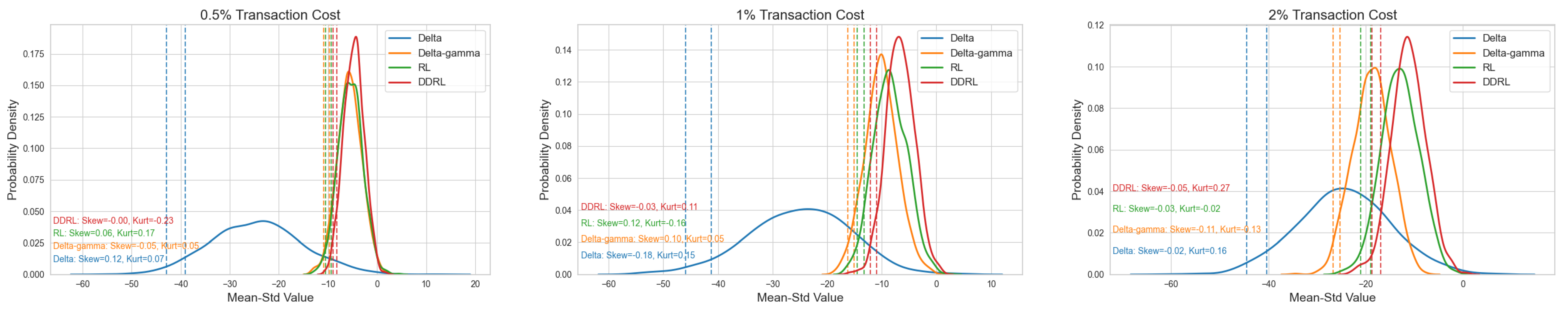
Figure 4.
Comparison of VaR-95 distribution for hedging under different transaction costs
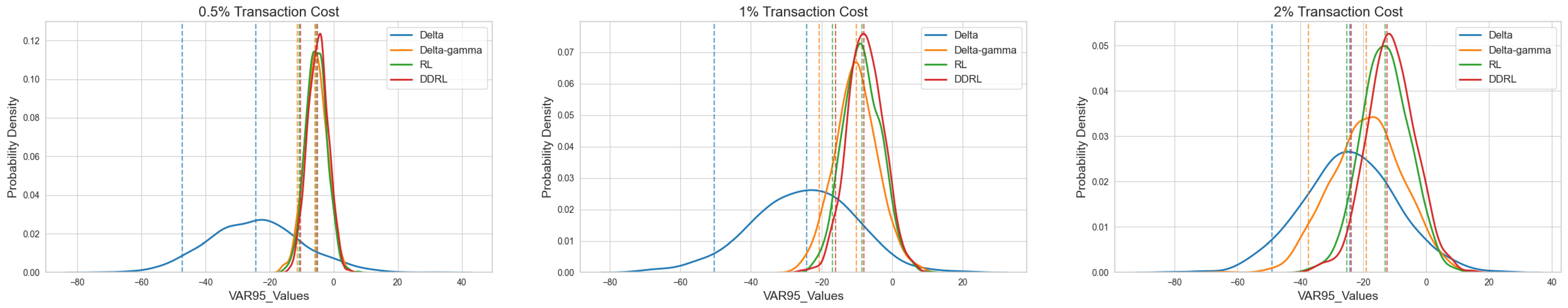
Figure 5.
Comparison of CVaR-95 distribution for hedging under different transaction costs
5.6. Risk Limit Management Evaluation
To reflect realistic trading constraints, we impose a gamma risk limit equal to 10% of the unhedged portfolio’s maximum gamma exposure, in line with industry practice. In all strategies, delta exposure is fully neutralized whenever it crosses a threshold, while gamma is hedged only when the exposure exceeds $50. This design enables a controlled evaluation of how different methods handle second-order risk without incurring unnecessary costs.
For the rule-based delta-gamma strategy, gamma hedging is triggered strictly based on this threshold. In contrast, the RL-based agents, particularly under the VaR95 objective, respond adaptively: when gamma exposure surpasses $50, they not only neutralize delta but also optimize gamma reduction in a cost-aware manner. This behavior reflects a learned trade-off between cost and risk, improving responsiveness compared to the fixed rule-based baseline.
As shown in Table 4, RL-based methods outperform the delta-gamma baseline across all objective functions and transaction cost levels, with DDRL consistently achieving the best results. For example, under 0.5% cost and the CVaR95 objective, DDRL reduces the objective value from 9.20 (delta-gamma) to 6.93, indicating superior risk-adjusted performance. These results demonstrate that learning-based strategies can maintain effective gamma control while dynamically adjusting hedging actions based on both risk sensitivity and cost efficiency.
5.7. Robustness Test
5.7.1. Robustness under Model Misspecification
In the initial experiments, we assumed that the hedging agent had accurate knowledge of the underlying asset’s stochastic process. However, in real-world trading scenarios, the assumed model often deviates from the actual market dynamics. To evaluate the robustness of the proposed strategies under model misspecification, we further examine the performance of various hedging strategies when the actual stochastic process differs from the one used for policy development.
Specifically, we assume a true market volatility process with a volatility of volatility parameter and an initial volatility of , which deliberately deviates from the model settings used during training. We systematically compare three classical rule-based strategies—Delta, Delta-Gamma, and Delta-Vega—with the RL-based RL and DDRL approaches under varying transaction costs (0.5%, 1%, 2%) and hedging horizons (30 days, 90 days).
Table 5 presents the complete comparison results. It can be observed that the risk metrics of traditional rule-based strategies deteriorate significantly with increasing transaction costs and extended horizons. For instance, under the 90-day horizon and 2% transaction cost scenario, the CVaR of the Delta-Gamma strategy reaches 65.05, while the Delta-Vega strategy shows an even higher CVaR of 84.38. In contrast, RL-based methods demonstrate clear advantages. DDRL consistently achieves the lowest Mean-Std, VaR95, and CVaR95 across all scenarios. For example, in the most challenging case with 2% transaction costs and a 90-day hedging horizon, DDRL yields a CVaR of only 30.73, significantly outperforming traditional approaches and demonstrating strong robustness and stability against model misspecification.
5.7.2. Robustness to Parameter Perturbations
Beyond model misspecification, we further assessed the sensitivity of DDRL to specific parameter variations. Since the true dynamics of the underlying asset may not be perfectly captured by the model used for training, it is essential to validate the strategy’s stability against perturbations in key stochastic parameters.
We considered two distinct stress-test scenarios. In the first scenario, the initial volatility is fixed at , while the volatility of volatility parameter v is varied across five values: 0, 0.15, 0.3, 0.45, and 0.6. In the second scenario, v is held constant at 0.3, while the initial volatility is varied across 10%, 20%, 30%, 40%, and 50%. Both scenarios involve 90-day options and a transaction cost rate of 1%.
Figure 6 illustrates the results of varying v, showing that the performance of DDRL—measured by Mean-Std, VaR95, and CVaR95—remains largely stable across different levels of volatility of volatility. This indicates that the strategy is not overly sensitive to changes in this parameter and maintains effective risk control.
Figure 7 provides a complementary view by showing the variation of the three objective functions under different initial volatility values . Each subfigure shows one of the three metrics plotted against the changing parameter. The curves in all cases show minimal fluctuation, reaffirming the robustness of the strategy to parameter uncertainty.
Overall, these tests confirm that DDRL delivers consistent and reliable hedging performance even under perturbations in key model parameters, enhancing its practical applicability in real-world trading scenarios.
6. Conclusions
We propose an innovative hedging framework designed to reduce risks in the complex world of finance. To address the challenges of environmental uncertainty and variability, we developed the DPN based on diffusion models and integrated it into SAC algorithm to create the DDRL algorithm for efficient hedging, accompanied by technical innovations that enhance the stability of the resulting hedging strategy. Extensive experimental results demonstrate the effectiveness of this algorithm. More importantly, the DPN algorithm holds potential applications for various optimization problems in financial scenarios. Furthermore, future research will focus on the following aspects: First, we will expand the applicability of the DDRL algorithm to other financial scenarios, such as dynamic asset allocation, portfolio optimization, and risk forecasting. This will help validate the algorithm’s generalizability and robustness across different financial environments. Next, we plan to incorporate additional market factors and macroeconomic indicators to further enhance the algorithm’s adaptability to complex market conditions. To ensure the practical operability of the algorithm, we will collaborate with financial institutions to conduct field testing and real-time applications, evaluating the algorithm’s performance under real market conditions.
Acknowledgments
The authors would like to thank the reviewers for their insightful comments and useful suggestions. The research is supported by the National Natural Science Foundation of China under Grant Nos. 62302400, 62225105, 62376227, Representative Graduate Research Achievement Cultivation Program of Southwestern University of Finance and Economics under Grant No. JGS2024041, and Guanghua Talent Project of Southwestern University of Finance and Economics.
References
- Jalilvand, M.; Bashiri, M.; Nikzad, E. An effective progressive hedging algorithm for the two-layers time window assignment vehicle routing problem in a stochastic environment. Expert Systems with Applications 2021, 165, 113877. [Google Scholar] [CrossRef]
- Guo, H.; Xi, Y.; Yu, F.; Sui, C. Time–frequency domain based optimization of hedging strategy: Evidence from CSI 500 spot and futures. Expert Systems with Applications 2024, 238, 121785. [Google Scholar] [CrossRef]
- Sun, H.; Feng, Y.; Meng, Q. Information dissemination behavior of self-media in emergency: Considering the impact of information synergistic-hedging effect on public utility. Expert Systems with Applications 2024, 252, 124110. [Google Scholar] [CrossRef]
- Chen, M.K.; Yang, D.Y.; Hsieh, M.H.; Wu, M.E. An intelligent option trading system based on heatmap analysis via PON/POD yields. Expert Systems with Applications 2024, 257, 124948. [Google Scholar] [CrossRef]
- Black, F.; Scholes, M. The pricing of options and corporate liabilities. Journal of political economy 1973, 81, 637–654. [Google Scholar] [CrossRef]
- Crépey, S. Delta-hedging vega risk? Quantitative Finance 2004, 4, 559–579. [Google Scholar] [CrossRef]
- Marzban, S.; Delage, E.; Li, J.Y.M. Equal risk pricing and hedging of financial derivatives with convex risk measures. Quantitative Finance 2022, 22, 47–73. [Google Scholar] [CrossRef]
- Buehler, H.; Gonon, L.; Teichmann, J.; Wood, B. Deep hedging. Quantitative Finance 2019, 19, 1271–1291. [Google Scholar] [CrossRef]
- Qiu, Y.; Liu, R.; Lee, R.S. The design and implementation of a deep reinforcement learning and quantum finance theory-inspired portfolio investment management system. Expert Systems with Applications 2024, 238, 122243. [Google Scholar] [CrossRef]
- Carbonneau, A.; Godin, F. Deep equal risk pricing of financial derivatives with multiple hedging instruments. arXiv 2021, arXiv:2102.12694 2021. [Google Scholar]
- Fecamp, S.; Mikael, J.; Warin, X. Deep learning for discrete-time hedging in incomplete markets. Journal of computational Finance 2020, 25. [Google Scholar] [CrossRef]
- Williams, R.J. Simple statistical gradient-following algorithms for connectionist reinforcement learning. Machine learning 1992, 8, 229–256. [Google Scholar] [CrossRef]
- Kim, H. Deep hedging, generative adversarial networks, and beyond. arXiv 2021, arXiv:2103.03913. [Google Scholar]
- Assa, H.; Kenyon, C.; Zhang, H. Assessing reinforcement delta hedging. Available at SSRN 3918375 2021. [Google Scholar] [CrossRef]
- Mikkilä, O.; Kanniainen, J. Empirical deep hedging. Quantitative Finance 2023, 23, 111–122. [Google Scholar] [CrossRef]
- Silver, D.; Lever, G.; Heess, N.; Degris, T.; Wierstra, D.; Riedmiller, M. Deterministic policy gradient algorithms. In Proceedings of the International conference on machine learning. Pmlr; 2014; pp. 387–395. [Google Scholar]
- Fujimoto, S.; Hoof, H.; Meger, D. Addressing function approximation error in actor-critic methods. In Proceedings of the International conference on machine learning. PMLR; 2018; pp. 1587–1596. [Google Scholar]
- Marzban, S.; Delage, E.; Li, J.Y.M. Deep reinforcement learning for option pricing and hedging under dynamic expectile risk measures. Quantitative Finance 2023, 23, 1411–1430. [Google Scholar] [CrossRef]
- Cao, J.; Chen, J.; Farghadani, S.; Hull, J.; Poulos, Z.; Wang, Z.; Yuan, J. Gamma and vega hedging using deep distributional reinforcement learning. Frontiers in Artificial Intelligence 2023, 6, 1129370. [Google Scholar] [CrossRef]
- Zheng, C.; He, J.; Yang, C. Option Dynamic Hedging Using Reinforcement Learning. arXiv 2023, arXiv:2306.10743. [Google Scholar]
- Ozbayoglu, A.M.; Gudelek, M.U.; Sezer, O.B. Deep learning for financial applications: A survey. Applied soft computing 2020, 93, 106384. [Google Scholar] [CrossRef]
- Lillicrap, T.P.; Hunt, J.J.; Pritzel, A.; Heess, N.; Erez, T.; Tassa, Y.; Silver, D.; Wierstra, D. Continuous control with deep reinforcement learning. arXiv 2015, arXiv:1509.02971. [Google Scholar]
- Haarnoja, T.; Zhou, A.; Abbeel, P.; Levine, S. Soft actor-critic: Off-policy maximum entropy deep reinforcement learning with a stochastic actor. In Proceedings of the International conference on machine learning. Pmlr; 2018; pp. 1861–1870. [Google Scholar]
- Ursone, P. How to calculate options prices and their greeks: exploring the black scholes model from delta to vega; John Wiley & Sons, 2015. [Google Scholar]
- Xiao, B.; Yao, W.; Zhou, X. Optimal option hedging with policy gradient. In Proceedings of the 2021 International Conference on Data Mining Workshops (ICDMW); IEEE, 2021; pp. 1112–1119. [Google Scholar]
- Halperin, I. Qlbs: Q-learner in the black-scholes (-merton) worlds. arXiv 2017, arXiv:1712.04609. [Google Scholar] [CrossRef]
- Kolm, P.N.; Ritter, G. Dynamic replication and hedging: A reinforcement learning approach. The Journal of Financial Data Science 2019, 1, 159–171. [Google Scholar] [CrossRef]
- Du, J.; Jin, M.; Kolm, P.N.; Ritter, G.; Wang, Y.; Zhang, B. Deep reinforcement learning for option replication and hedging. The Journal of Financial Data Science 2020, 2, 44–57. [Google Scholar] [CrossRef]
- Vittori, E.; Trapletti, M.; Restelli, M. Option hedging with risk averse reinforcement learning. In Proceedings of the Proceedings of the first ACM international conference on AI in finance, 2020, pp.
- Cao, J.; Chen, J.; Hull, J.; Poulos, Z. Deep hedging of derivatives using reinforcement learning. arXiv 2021, arXiv:2103.16409 2021. [Google Scholar] [CrossRef]
- Pham, U.; Luu, Q.; Tran, H. Multi-agent reinforcement learning approach for hedging portfolio problem. Soft Computing 2021, 25, 7877–7885. [Google Scholar] [CrossRef]
- Giurca, A.; Borovkova, S. Delta hedging of derivatives using deep reinforcement learning. Available at SSRN 3847272 2021. [Google Scholar] [CrossRef]
- Murray, P.; Wood, B.; Buehler, H.; Wiese, M.; Pakkanen, M. Deep hedging: Continuous reinforcement learning for hedging of general portfolios across multiple risk aversions. In Proceedings of the Third ACM International Conference on AI in Finance; 2022; pp. 361–368. [Google Scholar]
- Xu, W.; Dai, B. Delta-Gamma–Like Hedging with Transaction Cost under Reinforcement Learning Technique. The Journal of Derivatives 2022. [Google Scholar] [CrossRef]
- Cannelli, L.; Nuti, G.; Sala, M.; Szehr, O. Hedging using reinforcement learning: Contextual k-armed bandit versus Q-learning. The Journal of Finance and Data Science 2023, 9, 100101. [Google Scholar] [CrossRef]
- Fathi, A.; Hientzsch, B. A comparison of reinforcement learning and deep trajectory based stochastic control agents for stepwise mean-variance hedging. arXiv 2023, arXiv:2302.07996 2023. [Google Scholar] [CrossRef]
- Shavandi, A.; Khedmati, M. A multi-agent deep reinforcement learning framework for algorithmic trading in financial markets. Expert Systems with Applications 2022, 208, 118124. [Google Scholar] [CrossRef]
- Ulhaq, A.; Akhtar, N. Efficient diffusion models for vision: A survey. arXiv 2022, arXiv:2210.09292 2022. [Google Scholar]
- Du, H.; Zhang, R.; Liu, Y.; Wang, J.; Lin, Y.; Li, Z.; Niyato, D.; Kang, J.; Xiong, Z.; Cui, S.; et al. Beyond deep reinforcement learning: A tutorial on generative diffusion models in network optimization. arXiv preprint arXiv:2308.05384 2023, 3, 1661–1665. [Google Scholar]
- Wang, Z.; Hunt, J.J.; Zhou, M. Diffusion policies as an expressive policy class for offline reinforcement learning. arXiv 2022, arXiv:2208.06193 2022. [Google Scholar]
- Du, H.; Wang, J.; Niyato, D.; Kang, J.; Xiong, Z.; Kim, D.I. AI-generated incentive mechanism and full-duplex semantic communications for information sharing. IEEE Journal on Selected Areas in Communications 2023, 41, 2981–2997. [Google Scholar] [CrossRef]
- Hagan, P.S.; Kumar, D.; Lesniewski, A.S.; Woodward, D.E. Managing smile risk. The Best of Wilmott 2002, 1, 249–296. [Google Scholar]
Figure 1.
Dynamic Hedging Workflow.
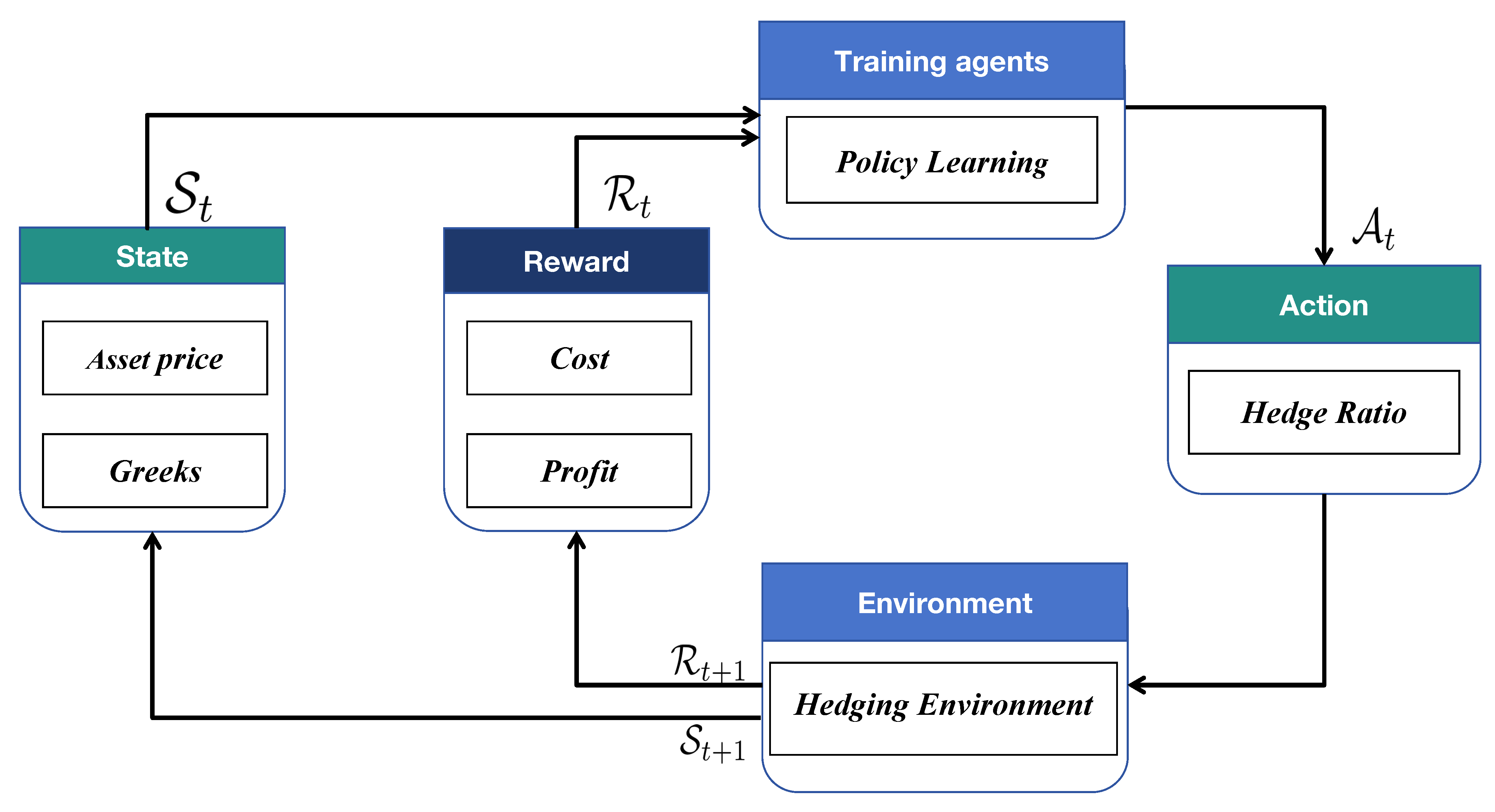
Figure 2.
DDRL Algorithm Architecture.
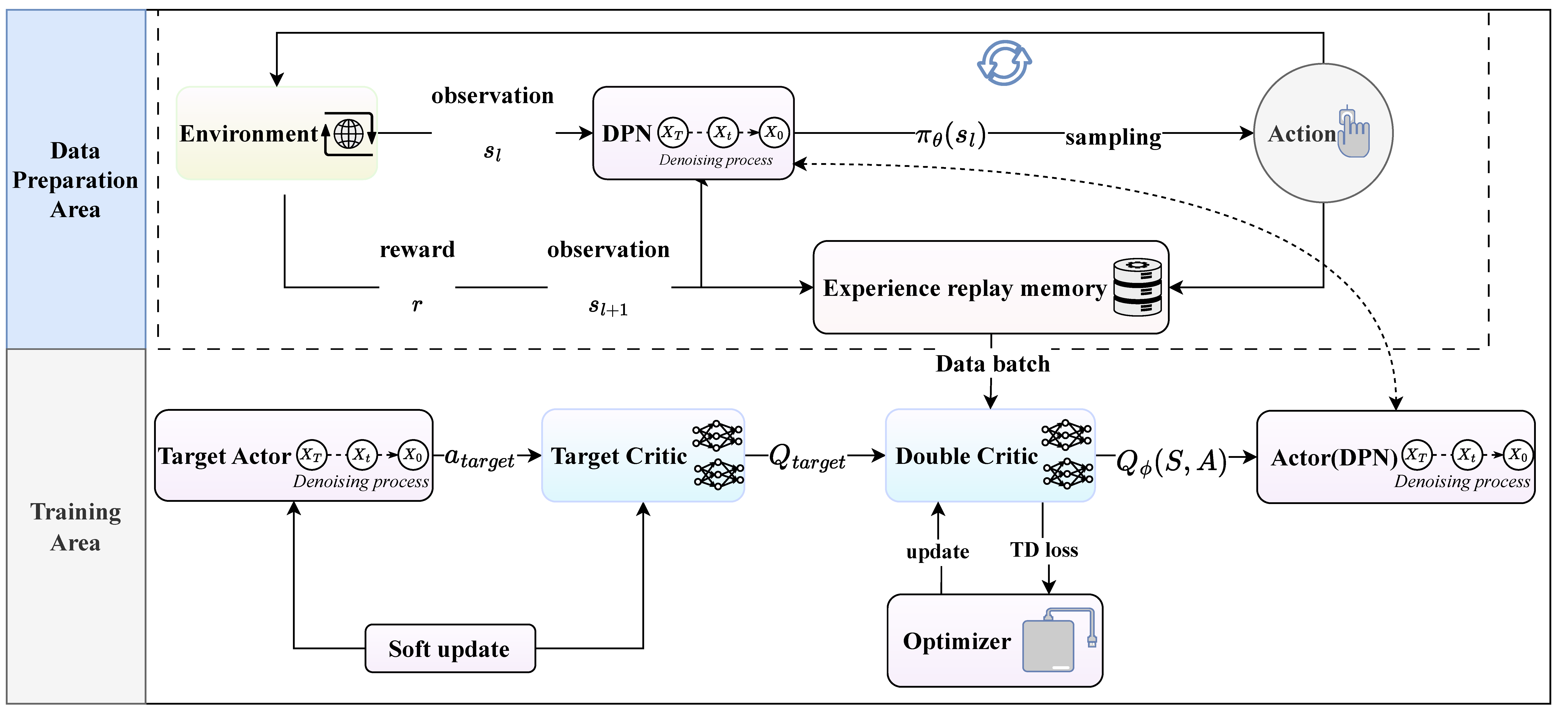
Figure 6.
Metrics vs. Volatility of Volatility (v)
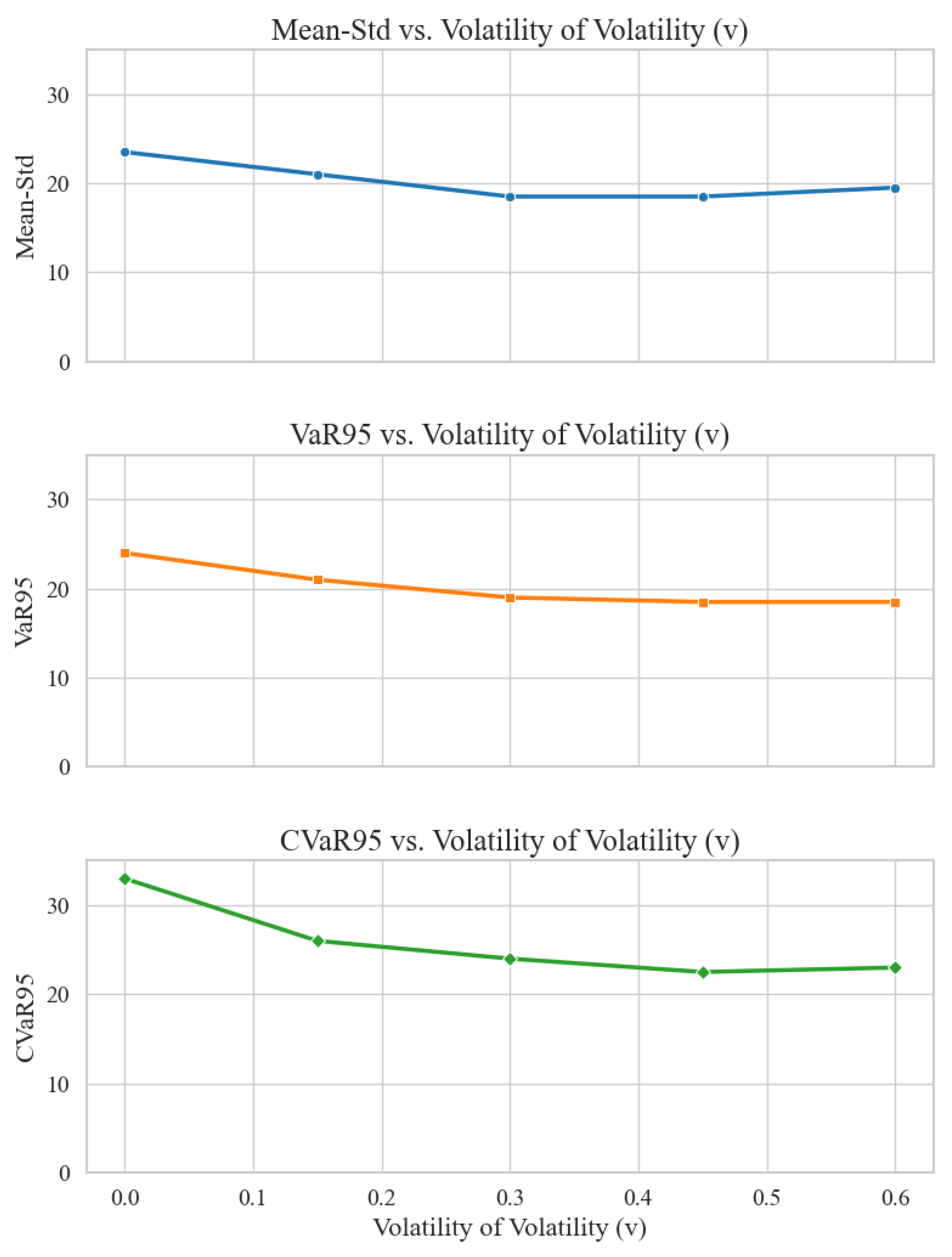
Figure 7.
Metrics vs. Initial Volatility ()


Table 1.
Summary of Analyzed RL Methods for Hedging.
| Source | Method | State | Action | Reward | Train Data | Test Data |
|---|---|---|---|---|---|---|
| [26] | Q-Learning | Disc. | GBM | GBM | ||
| [27] | SARSA | Disc. | GBM | GBM | ||
| [28] | DQN, PPO | Disc. | GBM | GBM | ||
| [29] | TRVO | Cont. | GBM | GBM | ||
| [30] | DDPG | Cont. | GBM, SABR | GBM, SABR | ||
| [31] | IMPALA | Disc. | HSX, HNX | HSX, HNX | ||
| [32] | DQN, DDPG | Disc. | GBM, Heston | GBM, Heston, S&P | ||
| [25] | Policy Gradient w/ Baseline | Disc. | GBM, Heston | GBM, Heston, S&P | ||
| [13] | Direct Policy Search | Cont. | CVaR | GBM, GAN | GBM, GAN | |
| [14] | DDPG | Cont. | Payoff | Heston | Heston | |
| [33] | Actor-Critic | Cont. | S&P, DJIA | S&P, DJIA | ||
| [34] | DDPG | Cont. | S&P, DJIA | S&P, DJIA | ||
| [15] | TD3 | Cont. | CVaR | SABR | SABR | |
| [19] | D4PG-QR | Cont. | CVaR + mean-var | SABR | SABR | |
| [20] | DDPG, DDPG-U | Cont. | GBM, S&P | GBM, S&P | ||
| [35] | CMAB | Disc. | GBM | GBM | ||
| [36] | DDPG | Cont. | Min | GBM | GBM |
Notes: Method Abbreviations: SARSA (State–Action–Reward–State–Action); DQN (Deep Q-Network); PPO (Proximal Policy Optimization); TRVO (Trust Region Value Optimization); DDPG (Deep Deterministic Policy Gradient); TD3 (Twin Delayed Deep Deterministic Policy Gradient); D4PG-QR (Distributed Distributional Deep Deterministic Policy Gradient with Quantile Regression); IMPALA (Importance Weighted Actor-Learner Architecture); CMAB (Contextual Multi-Armed Bandit). State: denotes the underlying asset price at time t; is the remaining time to maturity; represents the implied volatility at time t; denotes the option price at time t; is the time step interval; K is the option strike price; and are the gamma and vega of the portfolio at time t, respectively; and are the gamma and vega of the hedge instruments; denotes the number of trading periods remaining until maturity; is the option delta at time t; is the time derivative of the option price. Action: Cont./Disc. indicate continuous/discrete action spaces. Reward: denotes portfolio value deviation at time t; represents the variance of portfolio value deviation, used as a risk penalty term; is the portfolio value at time t; denotes the variance of portfolio value; represents the standard deviation of portfolio value, used to measure risk; represents transaction costs at time t; is a regularization parameter controlling the trade-off between reward and risk or cost; CVaR refers to the Conditional Value at Risk; mean-var indicates a mean-variance objective. Data Sources: GBM (Geometric Brownian Motion), SABR (Stochastic Alpha Beta Rho model), Heston (Heston Stochastic Volatility Model), and GAN (Generative Adversarial Network) refer to synthetic data generation models used to simulate financial time series. S&P (Standard & Poor’s 500 Index), DJIA (Dow Jones Industrial Average), HSX (Ho Chi Minh Stock Exchange), and HNX (Hanoi Stock Exchange) refer to real-world financial market indices.
Table 2.
Experiment Settings.
| Item | Details |
|---|---|
| Underlying Asset | 100 units of the underlying asset, with a 50% chance of being long or short per order. |
| Option Contract Term | 60-day option contract. |
| Hedging Tool | 30-day at-the-money (ATM) option. |
| Order Arrival Process | Poisson process with a daily intensity of 1.0, resulting in one order per day on average. |
| Initial Stock Price | $10.00 |
| Annualized Volatility | 30% |
| Transaction Costs | 0.5%, 1%, and 2% of the option price. |
| Hedging Frequency | Daily hedging, dynamically adjusted based on market conditions. |
| Hedging Period | 30 days, using a 30-day ATM option. |
| Training Iterations | 50,000 iterations. |
| Evaluation Iterations | 10,000 iterations. |
| Number of Test Scenarios | Over 5,000 test scenarios, distinct from training scenarios. |
Table 3.
Results of tests when volatility is constant.
| Objective | Delta | Delta-gamma | RL | DDRL | R(RL) | R(DDRL) | IR | TCR |
|---|---|---|---|---|---|---|---|---|
| 0.5% transaction cost | ||||||||
| Mean-Std | 24.61 | 5.78 | 5.44 | 5.01 | 0.83 | 0.89 | 1.11% | 13.30% |
| VaR95 | 24.29 | 5.78 | 5.47 | 5.02 | 0.75 | 0.80 | 0.67% | 21.71% |
| CVaR95 | 36.64 | 7.13 | 6.78 | 5.99 | 0.79 | 0.85 | 0.75% | 31.53% |
| 1% transaction cost | ||||||||
| Mean-Std | 24.61 | 9.93 | 8.36 | 7.68 | 0.57 | 0.63 | 10.52% | 8.71% |
| VaR95 | 24.29 | 10.12 | 8.63 | 8.02 | 0.56 | 0.62 | 12.50% | 9.52% |
| CVaR95 | 36.64 | 11.55 | 10.02 | 9.27 | 0.60 | 0.67 | 11.70% | 17.50% |
| 2% transaction cost | ||||||||
| Mean-Std | 24.61 | 18.74 | 12.73 | 12.12 | 0.30 | 0.41 | 36.67% | 17.63% |
| VaR95 | 24.29 | 19.11 | 13.05 | 12.51 | 0.24 | 0.34 | 29.41% | 10.50% |
| CVaR95 | 36.64 | 21.10 | 15.37 | 14.96 | 0.29 | 0.38 | 37.93% | 19.37% |
Table 4.
Performance Comparison of Hedging Strategies under Gamma Risk Constraints.
| Transaction Cost | Objective Function | Delta-Gamma | RL | DDRL |
|---|---|---|---|---|
| 0.5% | Mean-Std | 7.27 | 6.80 | 5.01 |
| VaR95 | 7.40 | 6.43 | 6.02 | |
| CVaR95 | 9.20 | 7.84 | 6.93 | |
| 1.0% | Mean-Std | 9.59 | 9.19 | 9.01 |
| VaR95 | 9.69 | 8.86 | 8.12 | |
| CVaR95 | 11.62 | 10.39 | 9.68 | |
| 2.0% | Mean-Std | 14.85 | 13.34 | 12.51 |
| VaR95 | 15.17 | 13.29 | 11.97 | |
| CVaR95 | 17.44 | 15.33 | 14.65 |
Table 5.
Performance under Stochastic Volatility.
| Hedge Maturity | Objective Function | Delta | Delta-Gamma | Delta-Vega | RL | DDRL |
|---|---|---|---|---|---|---|
| Transaction Costs = 0.5% | ||||||
| 30 days | Mean-Std | 35.76 | 19.46 | 44.82 | 17.76 | 15.27 |
| VaR95 | 34.43 | 19.23 | 42.90 | 19.31 | 18.53 | |
| CVaR95 | 52.91 | 27.53 | 62.77 | 26.06 | 24.77 | |
| 90 days | Mean-Std | 35.76 | 25.25 | 15.47 | 14.28 | 13.96 |
| VaR95 | 34.43 | 24.43 | 15.40 | 14.41 | 12.65 | |
| CVaR95 | 52.91 | 31.96 | 20.21 | 18.17 | 17.23 | |
| Transaction Costs = 1% | ||||||
| 30 days | Mean-Std | 35.76 | 23.06 | 51.36 | 20.03 | 17.99 |
| VaR95 | 34.43 | 23.02 | 50.24 | 20.22 | 18.89 | |
| CVaR95 | 52.91 | 31.55 | 69.92 | 26.81 | 21.23 | |
| 90 days | Mean-Std | 35.76 | 35.20 | 22.05 | 18.61 | 17.66 |
| VaR95 | 34.43 | 35.01 | 22.05 | 18.86 | 16.98 | |
| CVaR95 | 52.91 | 42.63 | 27.18 | 24.58 | 19.77 | |
| Transaction Costs = 2% | ||||||
| 30 days | Mean-Std | 35.76 | 30.51 | 64.77 | 24.17 | 21.31 |
| VaR95 | 34.43 | 30.67 | 64.56 | 23.85 | 19.89 | |
| CVaR95 | 52.91 | 39.79 | 84.38 | 31.57 | 28.75 | |
| 90 days | Mean-Std | 35.76 | 56.67 | 36.78 | 25.20 | 20.12 |
| VaR95 | 34.43 | 56.97 | 36.78 | 25.73 | 22.31 | |
| CVaR95 | 52.91 | 65.05 | 42.14 | 32.62 | 30.73 | |
Disclaimer/Publisher’s Note: The statements, opinions and data contained in all publications are solely those of the individual author(s) and contributor(s) and not of MDPI and/or the editor(s). MDPI and/or the editor(s) disclaim responsibility for any injury to people or property resulting from any ideas, methods, instructions or products referred to in the content. |
© 2025 by the authors. Licensee MDPI, Basel, Switzerland. This article is an open access article distributed under the terms and conditions of the Creative Commons Attribution (CC BY) license (http://creativecommons.org/licenses/by/4.0/).
Copyright: This open access article is published under a Creative Commons CC BY 4.0 license, which permit the free download, distribution, and reuse, provided that the author and preprint are cited in any reuse.


