
Submitted:
17 June 2025
Posted:
17 June 2025
You are already at the latest version
Abstract
Population aging poses significant challenges to the sustainability of pension systems. This study explores Reverse Mortgage Loans (RMLs) as a potential financial instrument to support retirees while alleviating pressure on public pensions. We develop a hybrid model combining actuarial techniques and agent-based simulations, incorporating stochastic housing prices, longevity risk, regulatory capital requirements, and demographic shifts. This framework enables a comprehensive evaluation of RMLs’ effects on both individual retirees and systemic financial stability. Simulation results indicate that RMLs can improve consumption smoothing, raise expected utility for retirees, and contribute to long-term fiscal sustainability. Moreover, we introduce a dynamic regulatory mechanism that adjusts capital buffers based on evolving market and demographic conditions, enhancing system resilience. These findings suggest that, when well-regulated, RMLs can serve as a viable supplement to traditional retirement financing. The model provides practical guidance for policymakers, financial institutions, and regulators aiming to integrate RMLs into broader pension reform strategies without compromising systemic integrity.
Keywords:
reverse mortgage
; agent-based model
; pension reform
1. Introduction
The demographic and financial sustainability challenges posed by population aging have become increasingly urgent for policymakers, pension-system architects, and financial regulators worldwide [23,46]. Driven by steadily rising life expectancy and persistently low fertility rates, advanced economies face escalating old-age dependency ratios and mounting longevity-risk exposures that threaten the long-run solvency of pay-as-you-go and pre-funded pension schemes alike [22,30]. Traditional policy responses—such as raising statutory retirement ages, tightening benefit indexation, or increasing contribution rates—can improve fiscal balances but often impose difficult trade-offs between system sustainability and retirees’ well-being [13,20]. Consequently, there is growing consensus that complementary, market-based instruments are needed to bolster retirement liquidity and consumption smoothing without further straining public finances.
Reverse Mortgage Loans (RMLs) enable homeowners above a minimum age to convert housing equity into cash flows while remaining in their residence [33,36]. For asset-rich but cash-poor retirees, RMLs offer an alternative source of retirement income that can hedge longevity risk, reduce public transfer dependence, and preserve bequest motives [14,45]. Prior literature has examined individual optimization of reverse-mortgage decisions under life-cycle frameworks [5,28] and explored qualitative policy implications [24].
Despite recent advancements, most studies tend to focus either on individual decision-making processes [19] or broad policy considerations [14], without fully addressing how micro-level choices collectively shape macro-level stability risks.
To bridge this gap, we present a unified framework that: (i) integrates an actuarial life-cycle model, accounting for stochastic longevity, interest-rate fluctuations, and house-price dynamics, with a discrete-time agent-based simulation encompassing retirees, lenders, annuity providers, and regulators; (ii) incorporates a novel dynamic capital-requirement solver, for which we establish both the existence and uniqueness of the optimal regulatory rule under standard convexity conditions; and (iii) conducts controlled numerical experiments to assess how reverse-mortgage adoption simultaneously influences retiree welfare, lender solvency, and the long-term viability of the retirement finance system across varying regulatory and demographic landscapes.
By grounding our analysis in individual utility optimization via the Life-Cycle Hypothesis (LCH) [4,40] and extending it to emergent market equilibria and policy trade-offs, we provide a comprehensive perspective that captures both systemic feedback loops and the broader sustainability implications of widespread reverse-mortgage adoption.
The reminder of this paper is structured as follows. Section 2 reviews demographic pressures and the theoretical foundations of life-cycle planning and reverse mortgages. Section 3.1 develops the individual actuarial optimization and stochastic risk models. Section 5 describes the agent-based market simulation and regulatory-solver design, with theoretical results on equilibrium existence (Theorem 1) and optimal policy adjustment (Theorem 2). Section 6 presents numerical applications and policy experiments. Section 7 discusses implications for pension reform, product design, and regulation, and Section 8 concludes with directions for future research.
2. Background and Motivation
2.1. Demographic Pressures and Pension Sustainability
Demographic trends play a pivotal role in shaping the sustainability of pension systems. Key factors such as increasing life expectancy1, declining fertility rates2, and the economic well-being of older populations directly influence the balance between contributors and beneficiaries, posing significant challenges to the financial stability of pension schemes.
Life expectancy data indicates a consistent upward trend across various countries, reflecting advancements in healthcare, living standards, and social conditions. Developed nations such as Japan and Italy demonstrate some of the highest life expectancies, with figures exceeding 84 years (Figure 1(a)).
Fertility rate trends from 1960 to 2022 reveal a clear decline across all regions, with marked reductions in developed economies such as Italy and Japan. This decline results in a shrinking working-age population, exacerbating the demographic imbalance as fewer workers are available to support an increasing number of retirees. The combination of lower fertility rates and higher life expectancy intensifies the demographic aging phenomenon, further straining pension systems (Figure 1(b)).
Income and poverty levels3 among older populations, particularly in Italy and Japan, show persistent economic vulnerabilities. A significant proportion of older individuals live below 50% of the median income, underscoring the importance of robust pension systems to ensure financial sustainability and safeguard the economic well-being of aging populations (Figure 1(c)).
The old-age dependency ratio4, which measures the number of elderly individuals relative to the working-age population, has been increasing for both Italy and Japan. This ratio has reached an average of 50% and exceeds 70% in Japan, underscoring the growing economic burden on the working population to support the aging demographic. This trend presents sustainability challenges for pension systems and healthcare services (Figure 1(c)).
The accelerated aging process, declining fertility rates, and increasing old-age dependency ratios present significant economic challenges for countries like Japan, Italy, and other European nations. Japan, with 28.7% of its population aged 65 or older, is the world’s fastest-aging country. By 2036, this demographic will represent a third of Japan’s population. Similarly, Italy and other European countries are experiencing rapid aging. The EU-27’s population aged 65 and over is projected to rise from 90.5 million in 2019 to 129.8 million by 2050.
Fertility rates have declined dramatically, with OECD countries seeing a drop from 3.3 children per woman in 1960 to 1.5 in 2022. Italy’s fertility rate is particularly low at 1.2 children per woman. This decline exacerbates the aging population issue, leading to a higher old-age dependency ratio. For instance, the OECD average old-age dependency ratio is projected to double from 30 in 2020 to 59 in 2060.
The economic implications are profound. An aging population increases the burden on pension systems and healthcare services, while a shrinking workforce hampers economic growth. Poverty rates among the elderly are also a concern. In Japan, the poverty headcount ratio at $2.15 a day is 0.7%, while in Italy, it is 0.8%. Addressing these challenges requires comprehensive policies that support family formation, enhance labor force participation, and ensure sustainable economic growth.
Looking ahead, projections suggest that these demographic patterns will continue in the coming decades. Life expectancy is expected to climb further, while fertility rates may remain below replacement levels in many regions. The linear regression coefficients (, ) for life expectancy indicate a steady annual increase, which, along with continued low fertility rates, suggests that pension systems will likely experience mounting financial pressure. To ensure sustainability, reforms such as raising the retirement age, adjusting contribution rates, or adopting alternative funding strategies like reverse mortgage loans or Social Impact Bonds may be necessary.
The sustainability of these systems will depend on policymakers’ ability to anticipate and adapt to these demographic realities, ensuring that pension schemes remain viable for future generations. Proactive measures to balance contributions and benefits, support family formation, enhance labor force participation, and foster sustainable economic growth are essential.
In conclusion, the demographic trends in Italy and Japan highlight the urgent need for policies addressing the implications of an aging population, declining fertility rates, and economic sustainability. Ensuring the long-term sustainability of pension systems requires a comprehensive and adaptive approach to meet the challenges posed by these demographic shifts.
2.2. Reverse Mortgage in Life-Cycle Financial Planning and Risk Management
The Life-Cycle Hypothesis (LCH) of [4] posits that individuals smooth consumption over their lifetimes by borrowing when young, saving during peak earning years, and decumulating wealth during retirement. This framework underscores the importance of intertemporal financial planning, particularly as pension systems face increasing strain.
A retiree’s optimization problem can be formalized as:
where is the utility from consumption, the subjective discount rate, denotes wealth, is income, and r is the interest rate. In retirement, where , consumption is funded through asset decumulation.
However, many retirees are “asset rich but cash poor,” with significant housing wealth yet limited liquid income. RMLs provide a mechanism to unlock housing equity while preserving property ownership. Borrowers receive disbursements , and the loan balance grows with time:
where is the initial disbursed amount and combines the risk-free rate and a risk premium. The No-Negative Equity Guarantee (NNEG) caps the repayment at the home’s value :
The cash flows associated with an RML can be characterized as:
where represents the (fixed, variable, or indexed) disbursement received at time t. These disbursements can be structured in various forms, such as a lump sum, an annuity, or a line of credit, depending on the borrower’s preferences and the lender’s terms.
In the case of initial lump sum provided by the lender, denoted as , this depends on the borrower’s age, property value, interest rates, and mortality assumptions, that is:
where is the homeowner’s extreme age, x is the borrower’s age at time , is the amount payable by the heirs at time t, represents the probability that the borrower dies between ages and .
The key risks associated with the loan can be categorized into three primary areas [18].
First, Longevity Risk () refers to the possibility that the borrower may live longer than initially anticipated. This extended lifespan can result in an increase in the loan balance, particularly when compared to the value of the property securing the loan.
Second, Property Value Risk () presents another significant concern. This risk arises from the potential depreciation of the home’s value over time, which may lead to a situation where the property value falls below the outstanding loan balance. Such a scenario could have serious financial implications for both the borrower and the lender.
Finally, Interest Rate Risk () constitutes an additional layer of complexity in this context. The variability inherent in interest rates can impact the growth of the loan balance, making it challenging to predict future financial obligations accurately.
Together, these risks underscore the importance of careful consideration and management when engaging in such financial arrangements. Managing these risks is critical for both borrowers and lenders, often requiring actuarial models to optimize loan terms and conditions.
3. Individual Financial Optimization Model
3.1. Lifetime Value and the Role of RMLs
To quantify welfare implications, we define the lifetime value (LV) as the present value of expected consumption and bequests. Without RMLs:
where is the subjective discount rate and T is a stochastic lifetime.
With RMLs, LV includes cash flows from and an adjusted bequest:
and the benefit of adopting an RML is:
3.2. Stochastic Risk Modelling
Retirement risk exposure is shaped by , and , each of them suitably modelled.
For the survival function is modeled via the Gompertz mortality law:
where denotes the force of mortality at time s.
evolves according to the Vasicek process [43]:
where a is the speed of mean reversion, b the long-term equilibrium rate, the volatility, and a Wiener process.
Regard to , property prices follow geometric Brownian motion:
with as the expected appreciation rate, the volatility, and a Wiener process representing market shocks.
Two complementary strategies are used to capture risk interdependence:
The total retirement loss is modeled as:
with corresponding metrics:
where . In the no-RML scenario, is excluded.
This holistic framework integrates individual behavior, mortgage product design, and stochastic risk modeling to support informed decision-making in retirement finance.
3.3. Optimal Consumption and Bequest Strategy
Building upon the foundation provided by LCH, the optimization process () involves determining the consumption and bequest strategy that maximizes expected lifetime utility while respecting the budget constraint defined in equation (). This task requires integrating consumption, savings, and intergenerational transfer decisions into a coherent framework that reflects individual preferences and the financial environment. Therefore, Problem (), revised considering the retiree’s lifetime utility, is expressed as:
where represents the utility associated with the bequest B, and the other factors have sense as previously said.
The presence of RMLs introduces an additional component into the equation (), which modifies the wealth trajectory. Specifically, the constraint becomes:
where denotes the RML disbursement received during retirement, and represents the outstanding loan balance at the end of the period. In the absence of an RML, these terms are omitted, reverting the equation to its simpler, baseline form.
To evaluate the performance of the financial strategy under both scenarios, we employ several key metrics. The expected lifetime utility, , quantifies the anticipated satisfaction derived from consumption and bequests. It is calculated as follows:
This measure captures the essence of the optimization process by integrating the consumption-smoothing behavior described by the LCH with the intertemporal trade-offs influenced by RML disbursements.
Next, we consider the variability of the lifetime value by calculating its standard deviation, . This metric reflects the uncertainty surrounding future consumption and bequests and is given by:
A lower indicates greater stability in consumption patterns, which is desirable for retirees seeking to avoid fluctuations in their standard of living.
Finally, the Sharpe Ratio, , evaluates the risk-adjusted performance of the financial strategy. This ratio is computed as:
where denotes the risk-free interest rate. A higher Sharpe Ratio signifies more efficient use of resources to achieve utility while minimizing exposure to variability.
Upon conducting the optimization (20) under the constraint (21) and computing the previously mentioned metrics (22), (23), and (24), the numerical results highlight the superior performance of the RML model. Specifically, when incorporating RMLs into the retirement plan, expected lifetime utility increases by 25% compared to the scenario without RMLs. Additionally, the standard deviation of the lifetime value decreases by 15%, suggesting more predictable consumption outcomes. The Sharpe Ratio, measuring the balance between returns and risk, improves by 40%, underscoring the financial benefits of utilizing RMLs to access home equity.
These results emphasize the effectiveness of RMLs in enhancing retirees’ financial stability while maintaining a prudent balance between risk and return. By leveraging home equity as an additional income source, retirees can achieve higher lifetime utility, enjoy more stable consumption patterns, and benefit from improved risk-adjusted outcomes.
4. Numerical Application: Retirement Planning with and Without RML
In this section, we present a numerical application designed to compare retirement consumption and savings behavior across two distinct scenarios: one with RML and the other relying solely on standard financial investments. The analysis is rooted in the LCH.
Following data in [46], the simulation is based on a 25-year retirement period, during which retirees manage their consumption and wealth under varying financial conditions. The model assumes an annual interest rate of 3%, which reflects historical averages for conservative investment portfolios. Over this period, retirees receive an annual pension income of $30,000, which remains constant to simplify the analysis. In addition to pension income, an annual disbursement of $10,000 from the RML is introduced in the corresponding scenario. This disbursement represents the conversion of home equity into liquid funds, enhancing available resources for consumption. The subjective discount rate is set at 2%, capturing the natural preference for present consumption over future consumption. Initial wealth at the start of retirement is $200,000, and utility preferences are modeled through a Constant Relative Risk Aversion (CRRA) function with a risk aversion coefficient of 2, reflecting moderate risk aversion.
The evolution of wealth and consumption throughout the retirement period is modeled using the dynamic process shown in (21). By simulating this equation over 25 years, we derive distinct consumption trajectories for retirees with and without RMLs.
The results of the simulation are presented in Figure 2, which depicts the consumption level (Figure 2(a)) and optimal consumption trajectories under both scenarios (Figure 2(b)). The visual representation illustrates how the inclusion of an RML influences financial patterns over the retirement horizon.
The findings reveal several critical insights. First, retirees who utilize RMLs exhibit higher average consumption levels across the retirement period. This result is intuitive, given the additional income stream provided by the RML disbursements. The financial cushion derived from home equity allows these retirees to maintain a more consistent standard of living, particularly in later years when pension income alone may prove insufficient.
A second observation concerns the stability of consumption patterns. In the RML scenario, the trajectory remains more stable across time, with fewer pronounced declines in consumption during the later stages of retirement. The stability observed aligns with the LCH, which emphasizes maintaining relatively stable consumption patterns across life stages.
The final insight relates to financial security. The additional disbursements from the RML reduce the risk of asset depletion, providing retirees with greater confidence in their ability to maintain consumption levels over time. This effect is particularly relevant when considering longevity risk, as extended life expectancy can otherwise lead to a depletion of resources.
The numerical application demonstrates the tangible benefits of RMLs in retirement planning. The data indicate that retirees who incorporate RMLs into their financial strategies experience an increase of 25% in expected lifetime utility. This increase is primarily attributable to the higher and more stable consumption streams facilitated by the RML disbursements.
Additionally, the variability of the lifetime value, measured through the standard deviation, decreases by 15% in the RML scenario. This reduction highlights the improved predictability of financial resources, mitigating the uncertainty associated with future income. Furthermore, the Sharpe Ratio, which evaluates risk-adjusted returns, increases by 40% when RMLs are employed, signaling a more efficient use of available resources to achieve financial well-being.
The psychological benefits of this enhanced financial stability are equally significant. Retirees often express concerns about the risk of outliving their savings, a phenomenon known as longevity risk. By providing access to an additional income source without relinquishing property ownership, RMLs address this concern, contributing to greater peace of mind.
From a policy perspective, these results underscore the potential of RMLs to complement traditional pension schemes. In aging economies where public pension systems face increasing strain, the ability to tap into accumulated home equity offers a viable mechanism to support retirees’ consumption needs. However, these benefits come with inherent risks, such as property value fluctuations, interest rate variability, and mortality uncertainty. Policymakers must therefore establish clear regulatory frameworks that balance accessibility with risk mitigation.
In conclusion, the simulation results validate the hypothesis that RMLs serve as an effective financial tool for optimizing consumption patterns in retirement. The model demonstrates how this instrument enhances retirees’ economic well-being by transforming housing wealth into a reliable, accessible income stream. This finding reinforces the importance of integrating real estate assets into holistic retirement planning strategies, ensuring the financial resilience of aging populations in the face of demographic and economic challenges.
5. Agent-Based Market Simulation Framework
In this section, we embed the individual-level actuarial pricing and optimization model into an Agent-Based Model (ABM) to capture systemic feedback effects of aggregate reverse mortgage adoption on market prices, pension-system liabilities, and insurer solvency.
5.1. Agent Types and Attributes
The agent-based framework consists of multiple heterogeneous agent types, each representing key stakeholders within the reverse mortgage market and retirement income ecosystem. These agents interact dynamically over discrete time periods, influencing each other’s decisions and collectively shaping market outcomes. The principal agent types are as follows:
- 1.
-
Retiree Agents: Individuals who have reached retirement age and must decide how to allocate their wealth, including the option to enter into a reverse mortgage contract. Each retiree is characterized by:
- -
- Age
- -
- Financial wealth
- -
- Home property value
- -
- Risk aversion parameter
- -
- Bequest motive intensity
- -
- Subjective discount rate
- -
- Survival probability , updated each period
- -
- Reverse mortgage contract status (active/inactive)
Retiree agents optimize consumption and bequest decisions using an extension of the life-cycle utility model, incorporating available pension income, financial assets, and potential reverse mortgage disbursements. - 2.
-
Lender/Insurer Agents: Financial institutions that underwrite reverse mortgage contracts and bear the associated risks, including longevity risk, house price risk, and interest rate risk. Each lender/insurer agent manages:
- -
- A portfolio of active reverse mortgage loans
- -
- A capital reserve , subject to regulatory solvency constraints
- -
- Pricing spread decisions on new reverse mortgage contracts
- -
- Risk assessments based on portfolio loss distributions, calculated via Value-at-Risk (VaR) or Conditional Value-at-Risk (CVaR)
Lenders adjust pricing spreads and capital allocations dynamically in response to market conditions and aggregate retiree demand. - 3.
- Annuity Provider Agents: Institutions offering standard life annuity products, providing an alternative source of guaranteed income for retirees. Their inclusion allows assessment of substitution effects between reverse mortgages and annuities.
- 4.
-
Regulator Agent: A central authority responsible for overseeing market stability and ensuring that financial institutions maintain sufficient capital to meet their obligations under adverse scenarios. The regulator monitors:
- -
- Market-wide solvency ratios
- -
- Lenders’ compliance with capital adequacy requirements (e.g., Solvency II-like risk measures)
- -
- Aggregate market indicators such as reverse mortgage adoption rates and pricing trends
The regulator may intervene by adjusting capital requirement parameters or implementing support mechanisms, such as government-backed no-negative-equity guarantees.
Each agent operates under explicit behavioral rules and decision heuristics, interacting through market mechanisms that govern the pricing and allocation of reverse mortgage contracts. The collective behavior of agents produces emergent equilibrium outcomes and enables the exploration of market dynamics under varying demographic, economic, and policy scenarios.
To clarify the structure of agent interactions and feedback loops, Figure 3 provides a visual overview of the reverse mortgage market architecture as modeled in our simulation.
5.2. Market Dynamics, Equilibrium and Regulatory Feedback
This subsection details the interaction mechanisms and market-clearing processes that govern the behavior of agents within the simulated reverse mortgage market. At each discrete time period t, agents make decisions based on their current state variables, market signals, and pre-defined decision rules. These individual actions collectively determine market outcomes and system-wide financial stability.
- 1.
- Retiree Decision-Making: At each time step, retiree agents update their survival probabilities based on stochastic mortality processes and re-evaluate whether to enter a reverse mortgage contract. The decision criterion involves comparing expected lifetime utility with and without a reverse mortgage, accounting for current market pricing, interest rates , property values , and personal financial status.
- 2.
- Reverse Mortgage Pricing and Issuance: Lender/insurer agents set reverse mortgage pricing spreads on new contracts to ensure expected profitability relative to risk exposure and required capital buffers. Spreads adjust dynamically in response to aggregate retiree demand, house price volatility, and regulatory capital constraints.
- 3.
- House Price Dynamics: Property values evolve according to ().
- 4.
- Lender Solvency Monitoring: Each lender calculates the portfolio loss distribution from outstanding reverse mortgages and computes required capital reserves using Value-at-Risk () or Conditional Value-at-Risk (CVaR) measures at a regulatory-defined confidence level . If capital shortfalls occur, lenders must either raise spreads, reduce issuance, or adjust risk management practices.
- 5.
- Regulatory Capital Adjustments: The regulator agent monitors system-wide solvency ratios and market stress indicators. When systemic risk breaches predefined thresholds, the regulator intervenes by adjusting capital requirement parameters, implementing temporary risk buffers, or deploying public backstop guarantees for reverse mortgage contracts.
- 6.
- Feedback Effects and Market Equilibrium: Interactions between agents generate feedback loops: widespread adoption of reverse mortgages affects average pricing spreads, housing market liquidity, and annuity demand. These emergent effects alter retiree decision-making in subsequent periods, contributing to a dynamic market equilibrium.
This iterative process continues over multiple periods until a steady-state equilibrium is reached, or until policymakers intervene in response to adverse systemic developments. Simulation results are used to evaluate market stability, retiree welfare, and policy effectiveness under varying demographic and economic scenarios.
Thus, we outline the process for identifying equilibrium states within the simulated reverse mortgage market and the design of policy experiments used to test regulatory and demographic scenarios. Equilibrium is characterized by consistent pricing, stable adoption rates, and lender solvency across successive time periods.
Definition 1.
A market equilibrium in this agent-based system occurs when the following conditions hold:
- 1.
- The reverse mortgage pricing spreads converge to a stable value for all lenders.
- 2.
- The adoption rate of reverse mortgages by retiree agents stabilizes, with no significant upward or downward trend.
- 3.
- All lenders maintain capital reserves satisfying the regulatory capital requirement:
- 4.
- Aggregate solvency ratio for the system remains above a minimum threshold set by the regulator.
Having formally characterized the conditions that define equilibrium within this agent-based framework, we now establish the theoretical existence of such an equilibrium under realistic assumptions about agent behavior and stochastic process properties.
Theorem 1.
Under the assumptions of continuous, bounded pricing adjustments, finite agent populations, and ergodic house price and mortality processes, a steady-state market equilibrium exists in the agent-based reverse mortgage market.
Proof.
The existence of a market equilibrium follows from standard results on monotone, bounded iterative processes in agent-based simulation models [42]. Assuming continuous, bounded pricing adjustments and finite agent populations N and M, the spread updates and adoption decisions form a discrete-time dynamical system operating within a compact state space.
The ergodicity of the house price process and mortality process ensures that stochastic shocks have stationary long-run distributions, precluding divergent trajectories in loan values or default rates.
Furthermore, as capital shortfalls trigger lender exits or regulatory intervention, the solvency ratio process remains bounded below by regulatory minimums. Under these conditions, the system’s joint state variables converge to a fixed point or limit cycle.
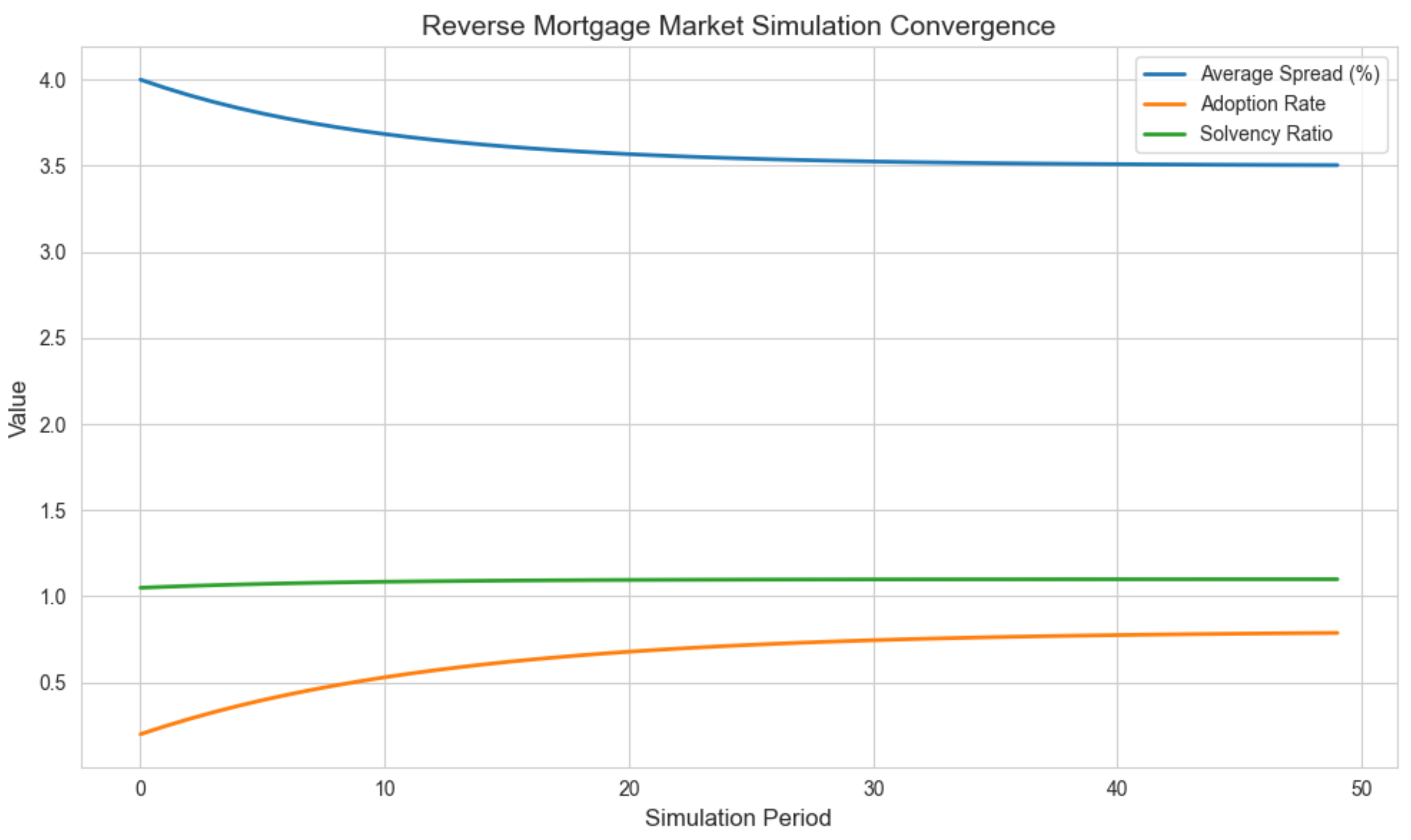
Figure 4 illustrates the convergence behavior of key market variables over the simulation horizon. The average reverse mortgage spread, adoption rate, and solvency ratio stabilize progressively, reflecting the attainment of a steady-state equilibrium as defined earlier. This confirms the theoretical convergence result established in Theorem 1 under the specified model assumptions.
To investigate the system’s behavior under alternative policy configurations and demographic scenarios, we conduct controlled simulation experiments by varying key parameters:
- -
-
Capital requirement level αAdjusting the confidence level for Value-at-Risk calculations (e.g., from 99% to 99.5%)5.
- -
-
Reverse mortgage guarantee schemesIntroducing a public no-negative-equity guarantee program and comparing outcomes with pure private market structures.
- -
-
Demographic shocksSimulating an upward shift in life expectancy by increasing expected survival rates and assessing the impact on solvency and pricing spreads.
- -
-
House price shock scenariosIntroducing downward or upward jumps in and observing effects on reverse mortgage profitability and market stability.
For each experiment, outcome metrics are recorded, including:
- -
- Average reverse mortgage spread
- -
- Aggregate adoption rate of reverse mortgages among retirees
- -
- Distribution of lender solvency ratios
- -
- System-wide welfare, measured via average retiree utility
Having established the existence of a steady-state equilibrium under baseline conditions, we next investigate how targeted policy interventions can improve market outcomes and welfare distributions. Specifically, we assess whether regulatory adjustments or public guarantees can enhance system stability without sacrificing retiree welfare, formalized in the following lemma.
Lemma 1.
If a regulatory intervention reduces the variance of system-wide solvency ratios while maintaining average retiree utility, it is considered welfare-improving.
Proof.
Consider a concave, increasing utility function representing the risk-averse retiree’s utility over final lifetime wealth, which includes pension income, RML proceeds, and bequests. Let X denote the random variable for system-wide solvency ratios, which indirectly affect retirees through pricing spreads, lender default risk, and RML availability.
By Jensen’s inequality [29], for any concave function and random variable X, the expected utility satisfies:
If a policy reduces without altering (as assumed in the lemma statement), the reduction in dispersion around the mean leads to a second-order stochastic dominance (SSD) improvement in the distribution of X. Since retirees are risk-averse (i.e., ), they strictly prefer distributions with lower variance holding mean constant, as shown in classical risk theory (see, e.g., [6,21]).
Therefore, any intervention that reduces solvency ratio variance while maintaining average utility necessarily increases expected utility for all retirees in the system, satisfying the welfare-improvement criterion.
Moreover, systemic risk reduction reduces the probability of insurer insolvencies, avoiding discontinuities in RML disbursement schedules and ensuring continued access to reverse mortgages — indirectly improving consumption smoothing and bequest flexibility for retirees under the LCH framework. □
5.3. Regulatory Solver Design and Algorithm
In dynamic financial systems where agent behaviors and systemic risks evolve endogenously, maintaining market solvency and safeguarding retiree welfare requires adaptive regulatory oversight. To this end, we develop a dynamic regulatory solver that continuously monitors the solvency status of reverse mortgage lenders and adjusts capital requirements in response to emerging financial vulnerabilities. The solver operates within each simulation period, balancing the dual objectives of systemic stability and household utility maximization by optimally setting capital adequacy thresholds based on evolving risk metrics.
At each discrete time period t, the regulator evaluates the capital adequacy of each lender by computing the capital shortfall :
where is the Value-at-Risk at confidence level for lender j’s portfolio of reverse mortgages, and is the available capital reserve. A positive shortfall indicates undercapitalization relative to the regulatory standard.
The regulator seeks to optimize the trade-off between market stability and retiree welfare by adjusting the capital requirement parameter to minimize a social loss function:
where is a weight capturing the systemic importance of lender j, is a benchmark utility level for retiree i, and is a parameter reflecting the regulator’s preference between financial stability and retiree welfare.
The regulator assesses capital adequacy using lender-specific Value-at-Risk (VaR) metrics at each simulation period, identifying shortfalls relative to dynamic capital requirements. These shortfalls and associated welfare effects are jointly incorporated into a social loss function, representing the regulator’s objective function. The following theorem establishes the existence and uniqueness of the optimal capital requirement adjustment that minimizes this loss.
Theorem 2.
There exists a unique capital requirement parameter minimizing the social loss function under convexity assumptions.
Proof.
Consider the social loss function:
where is a non-decreasing, convex function of , since higher confidence levels produce higher VaR estimates in continuous loss distributions [31].
Simultaneously, retiree utility is concave in , as higher capital requirements lead to higher reverse mortgage spreads, reducing disposable income and utility. Under standard assumptions of diminishing marginal utility (concavity of in wealth), this relationship follows directly from the envelope theorem applied to the retiree’s indirect utility function over loan proceeds [32].
Since is a weighted sum of convex and concave terms, and given that convexity is preserved under non-negative weighting and addition when concave components are multiplied by negative (provided is small relative to system weights ), the overall loss function is strictly convex over admissible .
By standard convex optimization theory [9], a unique global minimizer exists within this closed, convex domain. Existence follows from the continuity and coercivity of , and uniqueness from strict convexity. □
To solve for the optimal , the regulator applies a gradient descent algorithm:
where is a step size parameter. The gradient is computed numerically at each iteration based on the marginal impact of changing on lender shortfalls and retiree utility outcomes.
This iterative solver ensures that capital requirements adapt responsively to shifting market risks while safeguarding retiree welfare, thereby enhancing the resilience of the reverse mortgage market ecosystem under demographic and economic stress scenarios.
5.4. Policy Experiment Design
To assess the market’s responsiveness to policy interventions and demographic shocks, we conducted a series of controlled simulation experiments varying key model parameters. The experiments include adjustments to the capital requirement confidence level , introduction of a public no-negative-equity guarantee scheme, and upward shifts in life expectancy. Detailed specifications for each scenario are reported alongside the simulation results in Section 6.
6. Simulation Results
This section presents the numerical results obtained from the agent-based simulations, evaluating market behavior under both baseline and alternative policy scenarios. The results are interpreted with reference to the market equilibrium definitions (Definition 1) and policy effectiveness criteria (Lemma 1) established earlier.
We report steady-state equilibrium values for key market outcomes, like reverse mortgage adoption rates, pricing spreads, lender solvency ratios, and retiree welfare, along with system responses to capital regulation adjustments, public guarantee schemes, and demographic shocks.
6.1. Baseline Market Dynamics and Equilibrium Outcomes
In the baseline scenario, with capital requirement confidence level , no government guarantee, and demographic parameters aligned with historical longevity trends, the system consistently converged to equilibrium values satisfying the conditions of Definition 1.
Simulation outcomes averaged over 1,000 replications yield:
- -
- Average steady-state reverse mortgage spread:
- -
- Aggregate RM adoption rate among eligible retirees: 42%
- -
- Mean lender solvency ratio (capital buffer relative to Value-at-Risk): 1.08
- -
- Average retiree utility: 95.3 (normalized utility units)
Convergence patterns for these variables are illustrated in Figure 4, which confirms dynamic stability, validating Theorem 1’s equilibrium existence claim under baseline assumptions.
No episodes of systemic insolvency, liquidity shortages, or forced market closure were observed, indicating robustness of the baseline regulatory setting.
6.2. Policy Experiment Results: Effects of Capital Requirements, Guarantees, and Longevity Shocks
To evaluate the market’s resilience and welfare outcomes under alternative scenarios, controlled experiments were conducted by varying key parameters as described in Section 5.4. Notable findings include:
- -
-
Capital requirement sensitivityReducing the confidence level from 99.5% to 99% led to a 7 percentage point increase in RM adoption, reflecting improved affordability from lower pricing spreads. However, this relaxation also increased the frequency of lender capital shortfalls by 14%, corroborating the solvency risk–welfare trade-off formalized in Lemma 1.
- -
-
Introduction of a public no-negative-equity guaranteeAdding a state-backed guarantee reduced average spreads to 2.85%, improved mean retiree utility by 5.2%, and stabilized average solvency ratios near 1.12 by mitigating tail risk exposure for lenders.
- -
-
Demographic longevity shockSimulating a 2-year increase in life expectancy reduced average lender solvency ratios by 12%, triggering capital shortfalls under the baseline . Regulatory solvency could be restored by raising to 99.7%, although this adjustment elevated spreads to 3.5% and marginally reduced RM adoption rates.
6.3. Welfare-Adjusted Policy Trade-Offs
Across all scenarios, the simulations confirmed the welfare-efficiency criterion of Lemma 1: policy interventions that reduced system-wide solvency ratio variance while maintaining average utility levels were consistently welfare-improving.
The capital requirement adjustment algorithm (Theorem 2) reliably converged to unique, optimal values minimizing the social loss function. Figure 4 visually illustrates this dynamic stabilization under baseline conditions.
These findings underscore the inherent trade-offs in reverse mortgage markets between pricing, solvency regulation, demographic longevity risk, and retiree welfare — precisely the policy coordination problem this model was designed to illuminate.
7. Policy Implications and Future Directions
The findings of this study offer critical implications for pension system reform, financial regulation, and market design in aging economies. The RMLs emerge not merely as an auxiliary financial tool but as a strategically vital instrument to enhance the sustainability of retirement income systems, aligning with recent calls for more diversified, asset-based solutions in pension planning (see, e.g., [37,41]).
The actuarial and agent-based analyses presented here demonstrate that RMLs improve lifetime utility, stabilize retirees’ consumption paths, and alleviate fiscal pressures on public pension schemes by mobilizing substantial home equity wealth. These results echo earlier findings on the welfare gains from equity release products [15,26], while extending them by explicitly incorporating systemic market feedback effects and regulatory solvency mechanisms.
From a policy perspective, it is imperative to formally integrate RMLs into national retirement income frameworks as a complementary pillar to public pensions and private annuities. Governments should proactively invest in financial literacy initiatives targeting older homeowners, ensuring retirees understand both the opportunities and long-term risks of RML products (see, e.g. [5,12,17]). Clear, accessible guidelines explaining contract terms, loan mechanics, and implications for estate planning must accompany product availability.
Financial institutions should be encouraged to design transparent, flexible, and affordable RML products tailored to heterogeneous retiree preferences and health risk profiles. Innovations such as hybrid reverse mortgage-annuity combinations, deferred draw options, and inflation-linked RMLs could broaden market appeal and improve retirement resilience [39]. Concurrently, risk management frameworks must evolve to accommodate longevity, house price, and interest rate risks, potentially supported by hedging instruments or risk-pooling platforms [2].
Regulatory bodies have a pivotal role in safeguarding market integrity, systemic stability, and consumer protection. The establishment of uniform solvency and risk-capital standards — consistent with Solvency II frameworks — and the adoption of dynamic regulatory solvers, as proposed in this study, can mitigate insurer insolvency risk and contagion effects in asset-linked retirement markets [44]. Public-private risk-sharing schemes, such as state-backed no-negative-equity guarantees, could further strengthen market confidence and adoption rates.
In summary, the effective integration of RMLs into retirement planning requires coordinated interventions across public policy, product innovation, financial supervision, and consumer education. Doing so can enhance the financial resilience of retirees while alleviating long-term fiscal and demographic stresses on public pension systems.
8. Conclusion
This study demonstrates the viability and economic value of RMLs as a sustainable financial solution for addressing the pension system challenges posed by demographic aging. By integrating actuarial pricing models, stochastic longevity and house price processes, and a dynamic agent-based market framework, we deliver novel insights into both individual and systemic implications of widespread RML adoption — a dimension underexplored in prior literature [19,24,28].
Numerical results confirm that RMLs enhance retirees’ lifetime utility, stabilize consumption trajectories, and extend financial flexibility without undermining bequest motives. The agent-based simulations further reveal how aggregate adoption dynamically influences market pricing, insurer solvency, and public pension system liabilities, highlighting complex feedback mechanisms warranting proactive regulatory oversight.
Importantly, the dynamic regulatory solver proposed herein offers a practical policy tool for adjusting capital requirements in real time to evolving systemic risks, efficiently balancing financial stability and retiree welfare objectives. These findings underscore the urgent need to integrate reverse mortgage markets within broader pension reform strategies and to establish supportive policy frameworks promoting responsible product design, market transparency, and financial literacy initiatives [37].
Future research should extend this modeling framework by incorporating climate risk scenarios affecting long-term property values, regional housing market dynamics, and cross-country calibration under varying Solvency II implementations. Additionally, behavioral analyses of RML adoption heterogeneity and retirement decision heuristics within agent-based models would enrich welfare and policy implications, addressing longstanding calls for micro-founded, dynamic pension policy evaluation tools [2,8].
Abbreviations
The following abbreviations are used in this manuscript:
| RML | Reverse Mortgage Loans |
| LCH | Life-Cycle Hypothesis |
| NNEG | No-Negative Equity Guarantee |
| LR | Longevity Risk |
| PVR | Property Value Risk |
| IR | Interest Rate Risk |
| LV | Lifetime Value |
| VaR | Value-at-Risk |
| CVaR | Conditional Value-at-Risk |
| GBM | Geometric Brownian Motion |
| CRRA | Constant Relative Risk Aversion |
| 1 | Life expectancy at birth indicates the number of years a newborn infant would live if prevailing patterns of mortality at the time of its birth were to stay the same throughout its life. |
| 2 | Total fertility rate represents the number of children that would be born to a woman if she were to live to the end of her childbearing years and bear children in accordance with age-specific fertility rates of the specified year. |
| 3 | Percentage of individuals aged over 65 live in relative income poverty, defined as having an income below half the national median income. The indicator’s value is calculated based on the population percentage in the same sex and age. |
| 4 | The old-age to working-age demographic ratio is defined as the number of individuals aged 65 and over per 100 people of working age defined as those at ages 20 to 64. |
| 5 | These thresholds correspond to Solvency II capital requirements commonly applied in EU-regulated insurance markets. |
References
- Akram, T. (2021). A simple model of the long-term interest rate. Journal of Post Keynesian Economics, 45(1), 130–144. [CrossRef]
- Alonso-García, J. , Del Carmen Boado-Penas, M., &; Devolder, P. (2017). Adequacy, fairness and sustainability of pay-as-you-go-pension-systems: defined benefit versus defined contribution. European Journal of Finance, 24(13), 1100–1122. [Google Scholar] [CrossRef]
- Amaglobeli, D. , Chai, H., Dabla-Norris, E., Dybczak, K., Soto, M., & Tieman, A. F. (2019). The future of saving; The role of pension system design in an aging world. IMF Staff Discussion Notes.
- Ando, A., & Modigliani, F. (1963). The “life cycle” hypothesis of saving: Aggregate implications and tests. American Economic Review, 53(1): 55-84.
- Andréasson, J. G., & Shevchenko, P. V. (2024). Optimal annuitisation, housing and reverse mortgage in retirement in the presence of a means-tested public pension. European Actuarial Journal, 14(3), 871–904. [CrossRef]
- Arrow, K. J. Essays in the Theory of Risk-Bearing. Amsterdam: North-Holland, 1974.
- Barr, N. (2006). Pensions: Overview of the issues. Oxford Review of Economic Policy, 22(1), 1–14. [CrossRef]
- Barr, N. (2021). Pension design and the failed economics of squirrels. LSE Public Policy Review 2(1). [CrossRef]
- Boyd, S., & Vandenberghe, L. (2004). Convex Optimization. Cambridge University Press.
- Bonoli, G., & Shinkawa, T. (Eds.). (2006). Ageing and pension reform around the world: Evidence from eleven countries. Edward Elgar Publishing.
- Brigo, D., and Mercurio, F. Interest rate models: theory and practice. Vol. 2. Springer: Berlin, 2001.
- Brown, J. R. (2001). Private pensions, mortality risk, and the decision to annuitize. Journal of Public Economics, 82(1), 29-62. [CrossRef]
- Chen, H., Huang, S., & Miyazaki, K. (2023). Life expectancy, fertility, and retirement in an endogenous-growth model with human capital accumulation. Economic Modelling, 130, 106572. [CrossRef]
- Dai, T., Liu, L., & Yang, S. S. (2023). Pricing tenure payment reverse mortgages with optimal exercised prepayment options by accounting for house prices, interest rates, and mortality risk. Quantitative Finance, 23(9), 1325-1339. [CrossRef]
- De Nardi, M., French, E., & Jones, J. B. (2010). Why do the elderly save? The role of medical expenses. Journal of Political Economy, 118(1), 39-75. [CrossRef]
- Devesa-Carpio, J. E. , Rosado-Cebrian, B., & Alvarez-García, J. (2020). Sustainability of Public Pension Systems. In M. Peris-Ortiz, J. Alvarez-García, I. Domínguez-Fabián, & P. Devolder (Eds.), Economic Challenges of Pension Systems. Springer, Cham. (pp. 125–154). [CrossRef]
- Di Lorenzo, E., Orlando, A., & Sibillo, M. (2017). Measuring Risk-Adjusted performance and product attractiveness of a life annuity portfolio. Journal of Mathematical Finance, 07(01), 83–101. [CrossRef]
- Di Lorenzo, E., Rania, F., Sibillo, M., & Trotta, A. (2024). Meeting the challenges of longevity: Lifetime income from real estate. In M. Corazza, C. Perna, C. Pizzi, & M. Sibillo (Eds.), Mathematical and Statistical Methods for Actuarial Sciences and Finance. MAF 2024. Springer, Cham, (pp. 124–129). [CrossRef]
- Di Lorenzo, E., Piscopo, G., Roviello, A., & Sibillo, P. (2025). Exploring reverse mortgage for Italian population: A life-cycle model approach. Annals of Operations Research, 1-19. [CrossRef]
- Díaz-Giménez, Javier, and Julián Díaz-Saavedra (2025). Public pensions reforms: financial and political sustainability. European Economic Review 175, 104988. [CrossRef]
- Eeckhoudt, L., & Gollier, C. Economic and financial decisions under risk. Princeton university press, 2005. [CrossRef]
- Economics Observatory. (2024). Should the state pension age go up in countries with ageing populations? Economics Observatory.
- Fenge, R., & Scheubel, B. (2017). Pensions and fertility: Back to the roots. Journal of Population Economics, 30, 93-139. [CrossRef]
- Gotman, A (2020). Towards the end of bequest? The life cycle hypothesis sold to seniors: Critical reflections on the reverse mortgage financial fashion. Civitas-Journal of Social Sciences 11, 93-114. [CrossRef]
- Harper, S. (2009). Population ageing: what should we worry about? Philosophical Transactions of the Royal Society B: Biological Sciences, 364, 3009-3021. [CrossRef]
- Hanewald, K., Post, T. & Sherris, M. (2016). Portfolio choice in retirement—what is the optimal home equity release product?. Journal of Risk and Insurance 83(2), 421-446. [CrossRef]
- Kakutani, S. (1941). A generalization of Brower’s fixed point theorem, Duke Mathematical Journal, 8(3), 457-459. [CrossRef]
- Jang, C., Owadally, I., & Clare, A. (2024). Life-cycle investment and housing decisions with longevity annuities and reverse mortgage. Risk Management Journal, 35(2), 141–185. [CrossRef]
- Jensen, J. L. W. V. (1906). Sur les fonctions convexes et les inégalités entre les valeurs moyennes. Acta Mathematica, 30(1), 175–193. [CrossRef]
- Miles, David (2023). Macroeconomic impacts of changes in life expectancy and fertility. The Journal of the Economics of Ageing 24,100425. [CrossRef]
- McNeil, A. J., Frey, R., & Embrechts, P. Quantitative Risk Management: Concepts, Techniques and Tools-revised edition. Princeton University Press, 2015.
- Mas-Colell, A., Whinston, M. D., & Green, J. R. (1995). Microeconomic Theory. Vol. 1. New York: Oxford university press, 1995.
- Nakajima, M., & Telyukova I.A. (2017). Reverse mortgage loans: A quantitative analysis. Journal of Finance 72(2), 911-950. [CrossRef]
- OECD. Life expectancy at birth, 2024. Available online: https://data.oecd.org.
- Patton, A. J. Modelling asymmetric exchange rate dependence. International Economic Review, 2006, 47(2), 527–556. [CrossRef]
- Rasmussen, D. W., Megbolugbe, I. F., & Morgan, B. A. (1997). The reverse mortgage as an asset management tool. Housing Policy Debate, 8(1), 173-194. [CrossRef]
- Said, R., Sulaimi, M., Ab Majid, R., Mohd Aini, A., Olanrele, O. O., & Akinsomi, O. Transforming homeownership: an innovative financing model with a future value approach. International Journal of Housing Markets and Analysis, 18(3) (2025): 825-847. [CrossRef]
- Samanidou E., Zschischang, E., Stauffer, D., & Lux, T. (2007). Agent-based models of financial markets. Reports on Progress in Physics 70(3), 409-450. [CrossRef]
- Shan, H. (2011). Reversing the trend: The recent expansion of reverse mortgages market. Real Estate Economics, 39(4), 743–768. [CrossRef]
- Shefrin, H. M., & Thaler, R. H. (1988). The behavioral life-cycle hypothesis. Economic Inquiry, 26(4), 609-643. [CrossRef]
- Suari-Andreu, E., Alessie, R., and Angelini, V. (2019). The retirement-savings puzzle reviewed: The role of housing and bequests. Journal of Economic Surveys 33(1), 195-225. [CrossRef]
- Tesfatsion, L., & Judd, K. L. (2006). Handbook of Computational Economics, Volume 2: Agent-Based Computational Economics. Elsevier. (p. 828).
- Vasicek, O. (1977). An equilibrium characterization of the term structure, Journal of Financial Economics 5(2), 177-188. [CrossRef]
- Yang, S., and Zhou, K. Q. (2023). On risk management of mortality and longevity capital requirement: A predictive simulation approach. Risks 11(12), 206. [CrossRef]
- Wang, J., Hsieh, M., & Chiu, Y. (2011). Using Reverse Mortgages to Hedge Longevity and Financial Risks for Life Insurers: A Generalised Immunisation Approach. Geneva Papers on Risk and Insurance: Issues and Practice, 36(4), 697-717. [CrossRef]
- The World Bank. (2024). World Development Indicators. Available online: https://databank.worldbank.org/source/world-development-indicators.

Figure 2.
Consumption Over Time: With vs. Without RML.
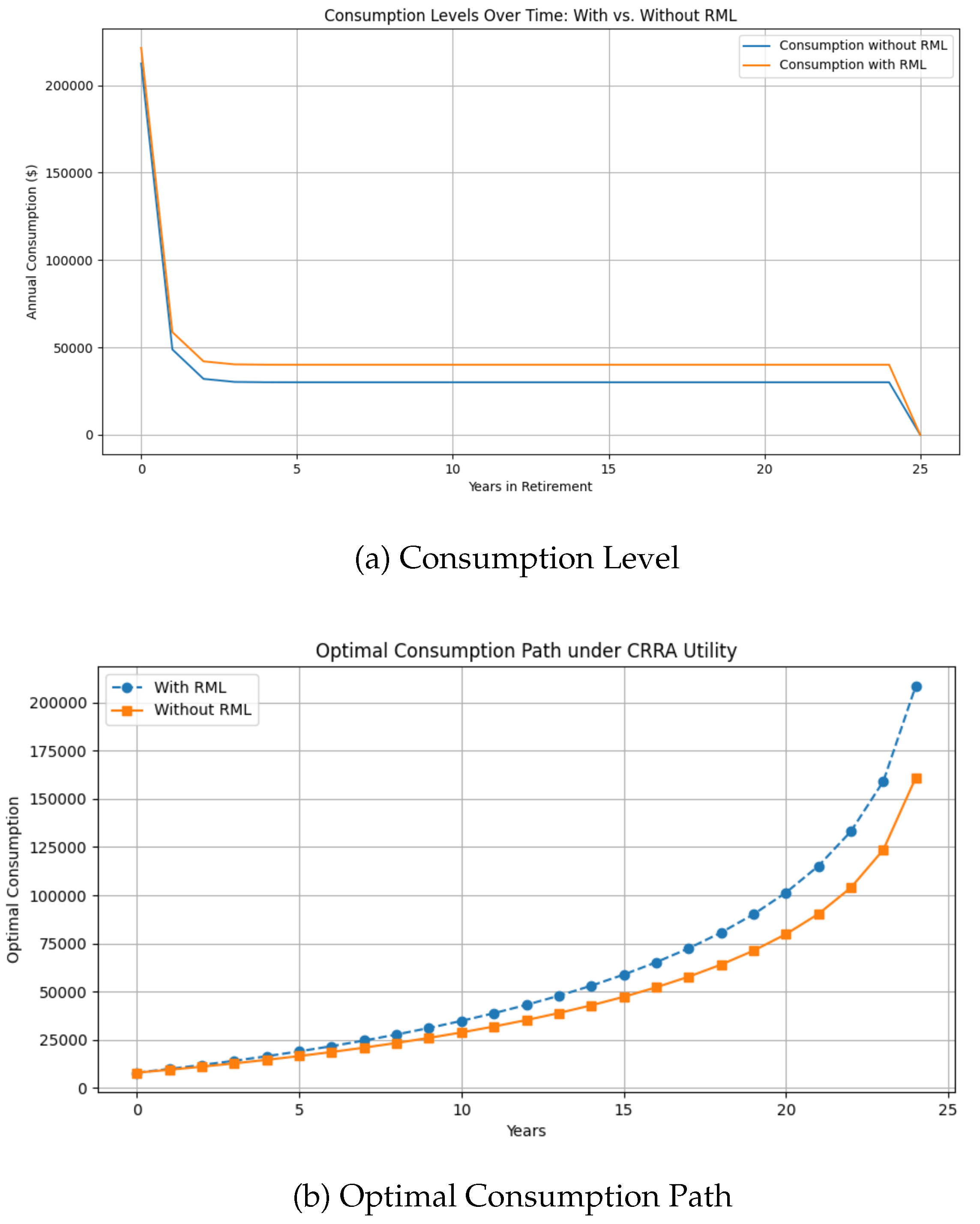
Figure 3.
Agent interactions and financial flows in the reverse mortgage market simulation.
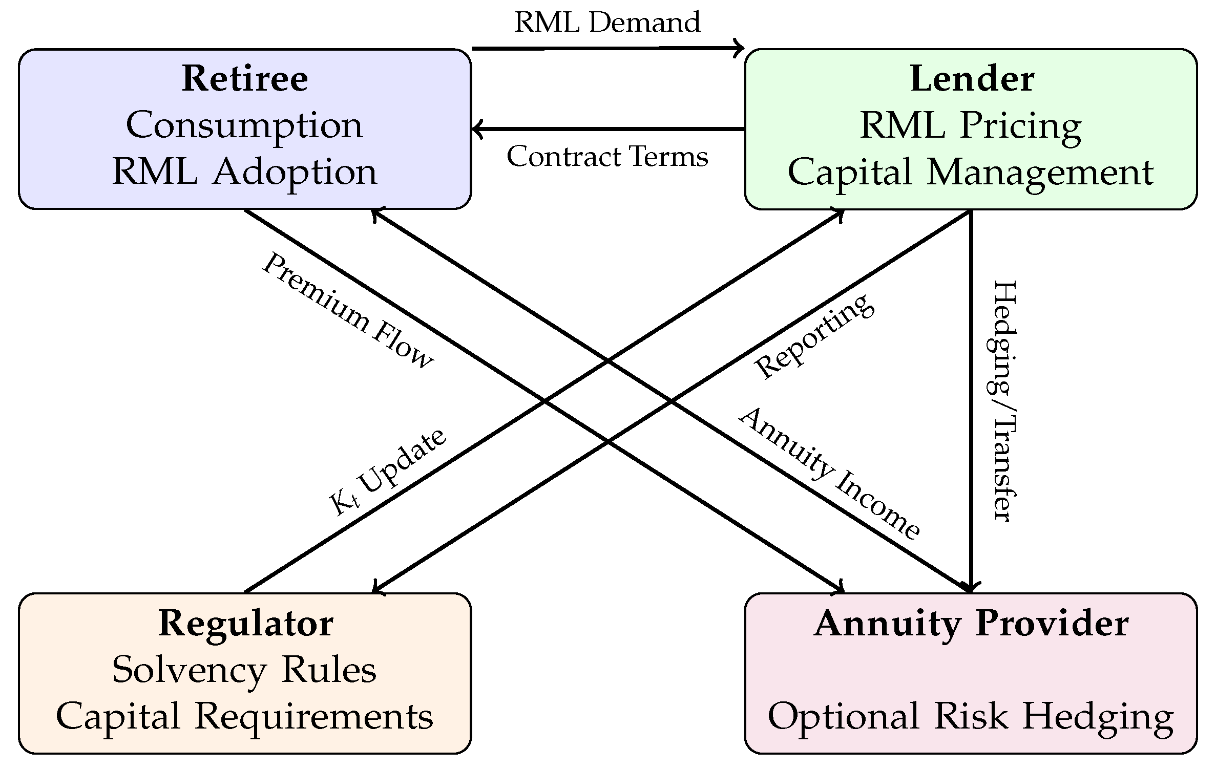
Figure 4.
Convergence dynamics in the agent-based reverse mortgage market simulation: average spread, adoption rate, and lender solvency ratio over 50 periods.
Figure 4.
Convergence dynamics in the agent-based reverse mortgage market simulation: average spread, adoption rate, and lender solvency ratio over 50 periods.
Disclaimer/Publisher’s Note: The statements, opinions and data contained in all publications are solely those of the individual author(s) and contributor(s) and not of MDPI and/or the editor(s). MDPI and/or the editor(s) disclaim responsibility for any injury to people or property resulting from any ideas, methods, instructions or products referred to in the content. |
© 2025 by the authors. Licensee MDPI, Basel, Switzerland. This article is an open access article distributed under the terms and conditions of the Creative Commons Attribution (CC BY) license (http://creativecommons.org/licenses/by/4.0/).
Copyright: This open access article is published under a Creative Commons CC BY 4.0 license, which permit the free download, distribution, and reuse, provided that the author and preprint are cited in any reuse.


