
Submitted:
13 June 2025
Posted:
16 June 2025
You are already at the latest version
Abstract
Contrastive learning improves model performance by differentiating between positive and negative sample pairs. However, its application is primarily confined to classification tasks, facing challenges with complex recognition tasks such as object detection and segmentation due to its limited capacity to capture spatial relationships and fine-grained features. To address this limitation, we propose LossTransform, a novel approach that redefines positive sample pairs and establishes a novel contrastive loss paradigm. LossTransform advances contrastive learning to the instance level, departing from the traditional sample level. Empirical evaluations on ImageNet, CIFAR, and object detection benchmarks indicate that LossTransform improves accuracy by +2.73% on CIFAR, +2.52% on ImageNet, and up to +5.2% in average precision on detection tasks, while maintaining efficiency. These results illustrate that LossTransform is compatible with large-scale training pipelines and exhibits robust performance across diverse and complex datasets.
Keywords:
loss function
; ensemble method
; repeated augmentation
; test-time augmentation
1. Introduction
Contrastive learning is instrumental in interpretable artificial intelligence as it enhances model performance by distinguishing between positive and negative pairs of samples. However, its practical applicability is limited. It performs well primarily in basic classification tasks on small datasets but struggles with more complex recognition tasks on larger datasets. Additionally, current studies [1,2] show that contrastive learning methods are not user-friendly, as they often require modifications to the original data pipeline, model architecture, and training recipe, instead of being directly applicable to existing models.
The application of contrastive learning is mainly limited to classification tasks due to its fundamental mechanism, which relies on unsupervised clustering, which brings positive sample pairs closer in the projection space while simultaneously maximizing the feature distance between negative sample pairs. Conventionally, the determination of whether two samples from a positive pair is based on two criteria: whether they originate from distinct augmentations of the same sample or whether they are separate sharing the same class label. However, this paradigm encounters challenges in more complex visual tasks such as object detection and semantic segmentation. These tasks not only involve category classification but also require the model to accurately localize objects spatially and capture fine-grained pixel-level information. The limitations of contrastive learning in these tasks arise from its inability to effectively manage multiple object instances and leverage local feature information.
To effectively apply contrastive learning in general recognition tasks, we have redefined the concept of positive sample pairs and designed a novel contrastive loss paradigm. Specifically, in object detection applications, our approach extends contrastive learning to facilitate object pairing at the instance level, thereby diverging from the conventional use of positive/negative image pairs. As shown in Figure 1, an image undergoes independent random data augmentations (e.g., flipping, translation, and cropping), resulting in multiple replicas. These replicas contain both common instances and potentially unique instances. The feature representation of an instance’s bounding box is subject to change after data augmentation. To align these common instances, we first apply an inverse data augmentation to restore these features to a unified space. Based on a self-supervised alignment mechanism, we use a greedy matching algorithm to subsequently select high-confidence positive instance pairs from the multiple image replicas. Finally, we minimize the Kullback–Leibler divergence to constrain the distance between these positive instance pairs, thereby ensuring that the representations of identical instances from different image replicas become more compact within the projection space.
In this study, we conduct extensive evaluations of LossTransform on various datasets, model architectures, and recognition tasks. Our ablation studies show that LossTransform enables models to achieve improvements during testing: a +2.73% accuracy increase on CIFAR [3] and a +2.52% accuracy increase on ImageNet [4]. Experiments using the multi-task loss functions of Faster R-CNN [5] and Mask R-CNN [6] produce similar results, with a +5.2% Average Precision (AP) improvement on PennFudanPed [7], a +0.8% mean Average Precision (mAP) increase on PASCAL VOC 2012 [8], and a +0.4% mAP increase on MS COCO [9].
2. Related Work
2.1. Test-Time Augmentation
The ensemble learning method [10] and test time augmentation (TTA) technique [11] are often used in evaluating neural networks for image classification [12,13,14]. These methods aggregate outputs from various models or data augmentations and compute the average predicted results as the final prediction. From the perspective of knowledge distillation [15], both methods serve as strategies for generating soft labels [16]. TTA is inherently more versatile than other ensemble voting methods in a production environment because it does not require multiple models during the prediction phase. Recently, researchers applied this method to post-processing the prediction and retraining models [15,17,18]. We have incorporated this method in the training process to minimize the gap between predictions and the anchor prediction.
2.2. Semi-Supervised Learning
Different from data augmentation techniques, Semi-supervised Learning (SSL) extends the cardinality of a training dataset by using a large amount of extra unlabelled data, subsequently generating pseudo labels through clustering algorithms [1,19]. In the SSL framework, the model can estimate the data-generating distribution and construct decision boundaries more precisely. An important concept in SSL is providing pseudo-labels to unlabeled data [20]. Building on this idea, in our method, if any images are successfully matched, they are collectively treated as positive samples of an unknown anchor sample. There is no requirement to identify the label of this unknown anchor sample; rather, we compute the average of the labels of all positive samples to serve as the pseudo-label for this anchor sample.
2.3. Random Augmentation Sampler
RASampler [21] is designed to limit data loading to a subset of the dataset for distribution purposes, incorporating repeated augmentation. For example, consider a dataset with five samples. To increase training data diversity, each sample can be augmented multiple times—here, three times per sample. The process typically involves:
- Shuffling: Shuffled the original dataset indices (e.g., [0, 1, 2, 3, 4]) to create a randomized order (e.g., [3, 1, 4, 0, 2]).
- Repetition: Repeating each index based on the augmentation count (e.g., three times) results in [3, 3, 3, 1, 1, 1, 4, 4, 4, 0, 0, 0, 2, 2, 2].
- Subsampling: Split the indices to create a subset (e.g., [3, 3, 1, 4, 4]).
We use RAsamper in LossTransform to ensure that examples are repeated multiple times in each iteration while the total number of examples seen by the model in each epoch remains unchanged.
3. Methods
Previous studies have relied heavily on minimizing the distance between positive pairs while maximizing the distance between negative pairs to improve model performance. This study demonstrates that substantial improvements in model performance can be achieved by employing LossTransdoem without the need to maximize the distance between negative pairs. In the following sections, we will take the task of object detection as an example: (1) defining the inverse transform for predicting the bounding box prediction; (2) explaining the instance alignment algorithm, which identifies all positive instance pairs through a greedy algorithm; (3) presenting LossTransform, which redefines the loss function in contrastive learning and extends its application to non-classification tasks, while maintaining efficacy in classification tasks.
3.1. Inverse Transform
While data augmentation methods do not change the category of an instance, they can significantly impact its bounding box specifically, when performing a horizontal flip (hflip) or translation on an image, the transformation of the bounding box follows these steps:
where and are the center coordinates, are the width and height respectively, W is the image width, and are the translation offsets in the horizontal ( x-axis) and vertical (y-axis) directions, respectively. The inverse transformation is straightforward as follows:
3.2. Instance Alignment
When training a model from scratch, pairing positive instances requires using the annotations to reorder all bounding boxes in replicas. For the predictions in the k-th replica:
It is important to note that a threshold must established to exclude instances that were removed from the original image due to data augmentation.
To pair the instances from the k-th and -th replicas, It is necessary first need to compute the area ratio of all bounding boxes in both replicas. If the ratio exceeds a predefined confidence threshold, the two replicas are considered to have been augmented from the same image. Subsequently, positive instance pairs will be matched by using the following greedy strategy:
3.3. Loss Transform
Given a loss function L, we propose LossTransform by incorporating an additional regularization component. For a mini-batch of predictions with corresponding targets , the model parameters are optimized by minimizing the following objective function:
where is a hyperparameter, represents the average prediction over all instances positively paired with , and is an indicator function applied element-wise to identify positive pairs.
4. Results
In this section, we start by evaluating the effectiveness of LossTransform in enhancing the generalizability of classifiers. Our experiments are primarily conducted on the CIFAR and ImageNet-1K datasets. Initially, we investigate the factors that affect the performance of LossTransform. Subsequently, we demonstrate that models trained with LossTransform yield more stable predictions. Additionally, we employ LossTransform methods on various datasets and classifiers for comparison with baselines. We then explore the applications of LossTransform in the fine-tuning process.
Next, we analyze the memory limitations of the LossTransform method. Due to the increased computational demand of duplicating sample replicas for data augmentation, training large models on datasets with large-scale images requires additional computational resources. To address this limitation, LossTransform-v1 is introduced, employing subsampling of Repeated Augment Sampling, thereby not increasing the computational resources required for model training. Consequently, it offers a feasible solution to the limitations of LossTransform. Experiments on ImageNet and Microsoft COCO reveal that fine-tuning pre-trained models with LossTransform-v1 can yield better evaluations than state-of-the-art baselines.
In our experiments, we adhere to the original training recipes of all benchmark models, including their optimizers, batch sizes, epochs, and learning rate schedules.
4.1. Training Benefits from LossTransform
4.1.1. Suitability for Complex Augmentation
Here, we verify that the LossTransform of Categorical Cross Entropy (CCE) works well across all data augmentation schemes. Table 1 presents a performance comparison between and the traditional CCE. For each combination of data augmentation schemes, we follow the official training recipe in the ResNet paper and apply CCE and for model training. All experiments are repeated five times with results variation under 0.3%. To emphasize general patterns, the best test error rates are highlighted in bold.
The last column of Table 1 demonstrates that is efficient for all hybrid data augmentation schemes. Empirically, while the traditional CCE-trained model shows improvement with a single data augmentation scheme, it fails under hybrid schemes due to the ambiguities introduced by mixed data augmentations. Our loss function overcomes this limitation to work for all data augmentation combinations and improve the model performance.
4.1.2. Faster Convergence
The LossTransform converts a loss function into a better form, thereby increasing the training speed and improving better model performance. Figure 2 shows a typical example of the CCE loss function, where models gain additional performance from the faster training on .
Based on CCE and official training recipe, the top-1 validation accuracy of DenseNet has stopped improving after 300 epochs. However, our loss function converges faster with 120 epochs. Figure 2 (left) illustrates the test error (%) of CCE-trained ResNet and -trained ResNet respectively, where saves 25% training iteration steps. Figure 2 (right) shows the same performance on DenseNet where saves 60% training iteration steps.
4.1.3. Stable Predictions
We demonstrate that classifiers trained using LossTransform have a significant change in the predictive behaviour. Figure 3 shows the difference between a plain-trained model and a LossTransform-trained model. The plain-trained model tends to assign inconsistent predicted probabilities to different augmented images, therefore the predicted results are easily affected by data augmentation (refer to Figure 3, left).
On the contrary, when we apply LossTransform, the model outputs almost identical predicted results to different augmented images (see Figure 3 right). This shows that the model trained with LossTransform is robust and minimally influenced by noise and data augmentation schemes.
4.1.4. The Number of Repetitions for Repeated Augmentation
To evaluate the impact of the number of repetitions m on model training, four distinct data augmentation techniques are used: affine transformation, horizontal flipping, CutMix, and mixup, with different values of m during training. For other training settings in our experiments, we follow the configurations outlined in the ResNet and DenseNet papers.
Figure 4 illustrates that the test accuracy reward of models is positively correlated with m. The model trained with tends to yield consistent improvement in accuracy with the growing m. Another factor that affects performance is the network complexity. The model with fewer parameters gains higher test accuracy improvement when training with the loss function.
4.1.5. Comparison with Other Loss Functions
Table 2 presents the comparison between the LossTransform and other methods when training models from scratch. We achieve better accuracies on all mini-size ResNet and DenseNet models without using extra training data or pre-trained models.
We also list in Table 2 the results of the large-scale ImageNet model (ResNet-50 with 25.6 million parameters) on the CIFAR dataset [2], the experiments of comparing cross-entropy training, SimCLR [1], maxi-margin classifiers [26], and SupCon [2]. In comparison, we achieve better results on smaller models, and our loss function only requires 120 epochs for training, while other methods are much more complicated (≈ 1000 epochs).
LossTransform is also suitable for fine-tuning. We conduct experiments using pre-trained MobileNet-V2 [27], NASNetMobile [28], and EfficientNet-B0 [29] models on the ImageNet-1K dataset. In these experiments, we still use the aforementioned simple data augmentation schemes for fair comparison. All models are trained end-to-end by SGD with a momentum of 0.9, a constant learning rate of 0.001, and 30 epochs. We use a batch size of 128 and set m for up to 4.
Table 3 shows the fine-tuning results of for deeper networks. The top-1 and top-5 accuracy refer to the model’s performance on the ImageNet-1K validation dataset. Remarkably, all the pre-trained models are downloaded from the TensorFlow platform. The real validation accuracy (without using any TTA and ensemble method) of these pre-trained models is much lower1 (MobileNetV2: 67.59%, NASNetMobile: 72.11%, EfficientNet-B0: 76.22%).
4.1.6. Object Detection and Instance Segmentation
Unlike image classification, object detection and instance segmentation are advanced tasks in computer vision. More specifically, object detection is a hybrid task of regression and classification that requires detecting objects of interest in unknown numbers. Instance segmentation needs to classify each pixel in the image to provide more fine analysis results. To date, most learning algorithms are still evaluated on benchmarks of classification tasks, so building a generalized algorithm that can traverse AI fields is an important challenge.
We investigate the application of LossTransform on PennFudanPed object detection and instance segmentation task. Table 4 shows the evaluation of models on the test set, we get significant improvements by using the new loss function , where is the plain multi-task loss function in Mask R-CNN. In this table, every pair of experiments uses the same training configurations, in which each model is trained by two different loss functions respectively. So the precision gain of models is entirely due to the LossTransform method.
In the first experiments, we replace the feature pyramid network2 [31] of Mask R-CNN architecture with different structures and retrain the whole model from scratch. For DenseNet121[14], GoogLeNet [32], ResNet-50 and WideResNet50 [33] -based FPNs, we set anchors as ((32,), (64,), (128,), (256,), (512,)) which means there are 5 levels/groups with 1 anchor size. For ConvNeXt-tiny [34], EfficientNetB4 [29], InceptionV3 [35], MNASNet1_0 [36], and ShuffleNetV2 [37] -based FPNs, we set anchors as ((32, 64, 128, 256, 512), (32, 64, 128, 256, 512)). These models are trained with a mini-batch size of 4 and a total of 18 epochs, with the learning rate divided by factor 10 at epochs 12 and 16. For DensNet121, EfficientNetB4, GoogLeNet, ResNet50, ShuffleNetV2, and WideResNet50, we start training with an initial learning rate of 0.01. Other models start with 0.0025.
In the last two experiments, we freeze the FPN and region proposal network [5] of the pre-trained Mask R-CNN model, then fine-tune it on the new dataset. The learning rate starts at 0.005.
We further investigate the PASCAL VOC 2012 dataset. In order to train the Mask R-CNN with LossTransfrom on this dataset, we need to convert the VOC to a dataset that can conduct the instance segmentation task. Here, we preprocess the dataset by using the algorithm [11,38] to split distinct individual instances from multiple objects of the same class. Then, we freeze the ResNet50-FPN and the region proposal network (RPN) of Mask-RCNN and use transfer learning to retrain the RoI heads. Finally, we achieve 73.5% mAP on the object detection task by training the model with , which gains an extra +0.8% mAP than using .
4.2. Fine-Tuning Benefits from LossTransform-v1
From Figure 1, it can be seen that the reformulated loss function in LossTransform consumes multiple times more memory during computation. For example, a mini-batch of images , after repetition and data augmentation, results in the actual training input , leading to a data throughput during optimization that is three times greater than in the standard training phase. This implies that LossTransform can effectively train large models on large-scale image datasets only if sufficient GPU memory is available.
To address this memory limitation, we apply RASampler in LossTransform. RASampler includes a shuffling and subsampling process. For instance, after sequentially applying shuffling, subsampling, and data augmentation, the actual mini-batch images become , ensuring that the number of examples the model learns from in each iteration remains unchanged.
We investigate the application of LossTransform-v1 on the ImageNet-1K classification (see Table 5) and MS COCO object detection (see Table 6) tasks. In our fine-tuning experiments, TorchVision provides multi-version pre-trained weights for each model architecture [39]. For fair ablation studies, we use the “V1 pre-trained weights" as the default since the corresponding training recipes for “V1 pre-trained weights" are not specifically tailored to each model architecture. We only keep the learning rate as the value from the last epoch in recipes. We empirically find that, when using LossTransform-v1, the model typically achieves performance improvement within 20 training epochs. Our experiments show that LossTransform is effective even for complex models like ViT [40].
5. Discussion
It is important to acknowledge the limitations of our method. Currently, we focus exclusively on image classification and object detection tasks. However, other recognition or generation tasks, such as text classification and causal language modeling, are also fundamentally classification problems. This suggests that our method may be applicable beyond the vision domain, though empirical validation is needed in future work.
In addition, our approach duplicates input data multiple times within each mini-batch to perform diverse data augmentations. While this strategy improves training dynamics, as shown in Section 4, it inevitably increases GPU memory consumption. Nonetheless, we observe that our method accelerates model convergence compared to standard training, which may offset the additional memory overhead over the course of training.
6. Conclusions
In this paper, we propose the LossTransform method for training neural networks. This method represents a more generalized approach to contrastive learning, which can be easily implemented through the reformulation of the loss function. It has proved to be effective across various data augmentation schemes, recognition tasks, and neural network architectures. The core principle of LossTransform is to minimize the distances between positive samples or pull together positive samples to their center.
LossTransform does not require the modification of data pipelines, model architectures, and training recipes. This method is user-friendly with a plug-and-play implementation, as it upgrades only the loss function in practical scenarios. It is applicable for either training from scratch and fine-tuning.
For model training, LossTransform contributes to improving the stability of model inference, boosting the convergence speed, and enhancing the efficiency of utilizing data augmentation. LossTransform-v1 addresses the shortcomings of LossTransform regarding memory constraints. In the case of challenging recognition tasks, LossTransform-v1 can continue to yield better evaluation than state-of-the-art baselines.
Abbreviations
The following abbreviations are used in this manuscript:
| AP | Average Precision |
| CCE | Categorical Cross Entropy |
| hflip | Horizontal Flip |
| mAP | Mean Average Precision |
| RA | Random Augmentation |
| RASampler | Random Augmentation Sampler |
| RPN | region proposal network |
| SSL | Semi-Supervised Learning |
| TTA | Test Time Augmentation |
References
- Chen, T.; Kornblith, S.; Norouzi, M.; Hinton, G. A simple framework for contrastive learning of visual representations. In Proceedings of the International conference on machine learning. PMLR; 2020; pp. 1597–1607. [Google Scholar]
- Khosla, P.; Teterwak, P.; Wang, C.; Sarna, A.; Tian, Y.; Isola, P.; Maschinot, A.; Liu, C.; Krishnan, D. Supervised contrastive learning. Advances in neural information processing systems 2020, 33, 18661–18673. [Google Scholar]
- Krizhevsky, A.; Hinton, G.; et al. Learning multiple layers of features from tiny images 2009.
- Russakovsky, O.; Deng, J.; Su, H.; Krause, J.; Satheesh, S.; Ma, S.; Huang, Z.; Karpathy, A.; Khosla, A.; Bernstein, M.; et al. Imagenet large scale visual recognition challenge. International journal of computer vision 2015, 115, 211–252. [Google Scholar] [CrossRef]
- Ren, S.; He, K.; Girshick, R.; Sun, J. Faster r-cnn: Towards real-time object detection with region proposal networks. Advances in neural information processing systems 2015, 28. [Google Scholar] [CrossRef] [PubMed]
- He, K.; Gkioxari, G.; Dollár, P.; Girshick, R. Mask r-cnn. In Proceedings of the Proceedings of the IEEE international conference on computer vision, 2017, pp.
- Shi, J.; et al. Penn-Fudan Database for Pedestrian Detection and Tracking. https://www.cis.upenn.edu/~jshi/ped_html/, 2007. Accessed: 2024-08-09.
- Everingham, M.; Van Gool, L.; Williams, C.K.; Winn, J.; Zisserman, A. The pascal visual object classes (voc) challenge. International journal of computer vision 2010, 88, 303–338. [Google Scholar] [CrossRef]
- Lin, T.Y.; Maire, M.; Belongie, S.; Hays, J.; Perona, P.; Ramanan, D.; Dollár, P.; Zitnick, C.L. Microsoft coco: Common objects in context. In Proceedings of the Computer Vision–ECCV 2014: 13th European Conference, Zurich, Switzerland, 2014, Proceedings, Part V 13. Springer, 2014, September 6-12; pp. 740–755.
- Dong, X.; Yu, Z.; Cao, W.; Shi, Y.; Ma, Q. A survey on ensemble learning. Frontiers of Computer Science 2020, 14, 241–258. [Google Scholar] [CrossRef]
- Shanmugam, D.; Blalock, D.; Balakrishnan, G.; Guttag, J. Better aggregation in test-time augmentation. In Proceedings of the Proceedings of the IEEE/CVF International Conference on Computer Vision, 2021, pp.
- Simonyan, K.; Zisserman, A. Very deep convolutional networks for large-scale image recognition. arXiv preprint arXiv:1409.1556, arXiv:1409.1556 2014.
- He, K.; Zhang, X.; Ren, S.; Sun, J. Deep residual learning for image recognition. In Proceedings of the Proceedings of the IEEE conference on computer vision and pattern recognition, 2016, pp.
- Huang, G.; Liu, Z.; Van Der Maaten, L.; Weinberger, K.Q. Densely connected convolutional networks. In Proceedings of the Proceedings of the IEEE conference on computer vision and pattern recognition, 2017, pp.
- Gou, J.; Yu, B.; Maybank, S.J.; Tao, D. Knowledge distillation: A survey. International Journal of Computer Vision 2021, 129, 1789–1819. [Google Scholar] [CrossRef]
- Galstyan, A.; Cohen, P.R. Empirical comparison of “hard” and “soft” label propagation for relational classification. In Proceedings of the International Conference on Inductive Logic Programming. Springer; 2007; pp. 98–111. [Google Scholar]
- Hinton, G.; Vinyals, O.; Dean, J.; et al. Distilling the knowledge in a neural network. arXiv preprint arXiv:1503.02531 2015, arXiv:1503.02531 2015, 22. [Google Scholar]
- Kim, I.; Kim, Y.; Kim, S. Learning loss for test-time augmentation. Advances in neural information processing systems 2020, 33, 4163–4174. [Google Scholar]
- Zbontar, J.; Jing, L.; Misra, I.; LeCun, Y.; Deny, S. Barlow twins: Self-supervised learning via redundancy reduction. In Proceedings of the International Conference on Machine Learning. PMLR; 2021; pp. 12310–12320. [Google Scholar]
- Athiwaratkun, B.; Finzi, M.; Izmailov, P.; Wilson, A.G. There are many consistent explanations of unlabeled data: Why you should average. arXiv preprint arXiv:1806.05594, arXiv:1806.05594 2018.
- Touvron, H.; Cord, M.; Douze, M.; Massa, F.; Sablayrolles, A.; Jégou, H. Training data-efficient image transformers & distillation through attention. In Proceedings of the International conference on machine learning. PMLR; 2021; pp. 10347–10357. [Google Scholar]
- Cubuk, E.D.; Zoph, B.; Shlens, J.; Le, Q.V. Randaugment: Practical automated data augmentation with a reduced search space. In Proceedings of the Proceedings of the IEEE/CVF Conference on Computer Vision and Pattern Recognition Workshops, 2020, pp.
- DeVries, T.; Taylor, G.W. Improved regularization of convolutional neural networks with cutout. arXiv preprint arXiv:1708.04552, arXiv:1708.04552 2017.
- Yun, S.; Han, D.; Oh, S.J.; Chun, S.; Choe, J.; Yoo, Y. Cutmix: Regularization strategy to train strong classifiers with localizable features. In Proceedings of the Proceedings of the IEEE/CVF international conference on computer vision, 2019, pp.
- Zhang, H.; Cisse, M.; Dauphin, Y.N.; Lopez-Paz, D. mixup: Beyond empirical risk minimization. arXiv preprint arXiv:1710.09412, arXiv:1710.09412 2017.
- Liu, W.; Wen, Y.; Yu, Z.; Yang, M. Large-margin softmax loss for convolutional neural networks. arXiv preprint arXiv:1612.02295, arXiv:1612.02295 2016.
- Howard, A.G.; Zhu, M.; Chen, B.; Kalenichenko, D.; Wang, W.; Weyand, T.; Andreetto, M.; Adam, H. Mobilenets: Efficient convolutional neural networks for mobile vision applications. arXiv preprint arXiv:1704.04861, arXiv:1704.04861 2017.
- Zoph, B.; Vasudevan, V.; Shlens, J.; Le, Q.V. Learning transferable architectures for scalable image recognition. In Proceedings of the Proceedings of the IEEE conference on computer vision and pattern recognition, 2018, pp.
- Tan, M.; Le, Q. Efficientnet: Rethinking model scaling for convolutional neural networks. In Proceedings of the International conference on machine learning. PMLR; 2019; pp. 6105–6114. [Google Scholar]
- Huang, Y.; Cheng, Y.; Bapna, A.; Firat, O.; Chen, D.; Chen, M.; Lee, H.; Ngiam, J.; Le, Q.V.; Wu, Y.; et al. Gpipe: Efficient training of giant neural networks using pipeline parallelism. Advances in neural information processing systems 2019, 32. [Google Scholar]
- Lin, T.Y.; Dollár, P.; Girshick, R.; He, K.; Hariharan, B.; Belongie, S. Feature pyramid networks for object detection. In Proceedings of the Proceedings of the IEEE conference on computer vision and pattern recognition, 2017, pp.
- Szegedy, C.; Liu, W.; Jia, Y.; Sermanet, P.; Reed, S.; Anguelov, D.; Erhan, D.; Vanhoucke, V.; Rabinovich, A. Going deeper with convolutions. In Proceedings of the Proceedings of the IEEE conference on computer vision and pattern recognition, 2015, pp.
- Zagoruyko, S.; Komodakis, N. Wide residual networks. arXiv preprint arXiv:1605.07146, arXiv:1605.07146 2016.
- Liu, Z.; Mao, H.; Wu, C.Y.; Feichtenhofer, C.; Darrell, T.; Xie, S. A convnet for the 2020s. In Proceedings of the Proceedings of the IEEE/CVF conference on computer vision and pattern recognition, 2022, pp.
- Szegedy, C.; Vanhoucke, V.; Ioffe, S.; Shlens, J.; Wojna, Z. Rethinking the inception architecture for computer vision. In Proceedings of the Proceedings of the IEEE conference on computer vision and pattern recognition, 2016, pp.
- Tan, M.; Chen, B.; Pang, R.; Vasudevan, V.; Sandler, M.; Howard, A.; Le, Q.V. Mnasnet: Platform-aware neural architecture search for mobile. In Proceedings of the Proceedings of the IEEE/CVF conference on computer vision and pattern recognition, 2019, pp.
- Zhang, X.; Zhou, X.; Lin, M.; Sun, J. Shufflenet: An extremely efficient convolutional neural network for mobile devices. In Proceedings of the Proceedings of the IEEE conference on computer vision and pattern recognition, 2018, pp.
- Fiorio, C.; Gustedt, J. Two linear time union-find strategies for image processing. Theoretical Computer Science 1996, 154, 165–181. [Google Scholar] [CrossRef]
- TorchVision Contributors. TorchVision Models. https://pytorch.org/vision/master/models.html, 2024. Accessed: 2024-08-09.
- Dosovitskiy, A.; Beyer, L.; Kolesnikov, A.; Weissenborn, D.; Zhai, X.; Unterthiner, T.; Dehghani, M.; Minderer, M.; Heigold, G.; Gelly, S.; et al. An image is worth 16x16 words: Transformers for image recognition at scale. arXiv preprint arXiv:2010.11929, arXiv:2010.11929 2020.
| 1 | The validation accuracy (MobileNet-V2: 71.3%, NASNetMobile: 74.4%, EfficientNet-B0: 77.1%) shown on the TensorFlow webpage and corresponding papers, are the results of ensemble and multi-crop models [30]. |
| 2 | As of v0.14, TorchVision offers the model architectures for ImageNet. We extract their backbone with feature pyramid network (FPN) on top of Mask R-CNN. |
Figure 1.
Contrastive learning applied to object detection. Image replicas are generated through Random Augmentation (RA), where each replica produces a series of bounding box via predictions. Inverse transformations are applied to these boxes to estimate the model’s predictions on the original image. Geometric and statistical methods are used to align instances and match positive pairs of boxes, followed by the computation of an anchor box by averaging the corresponding box pairs. The KL divergence is minimized to reduce the distance between each predicted box and its anchor. Finally, anchor boxes are transformed and concatenated with unpaired bounding boxes to obtain the optimized box predictions as .
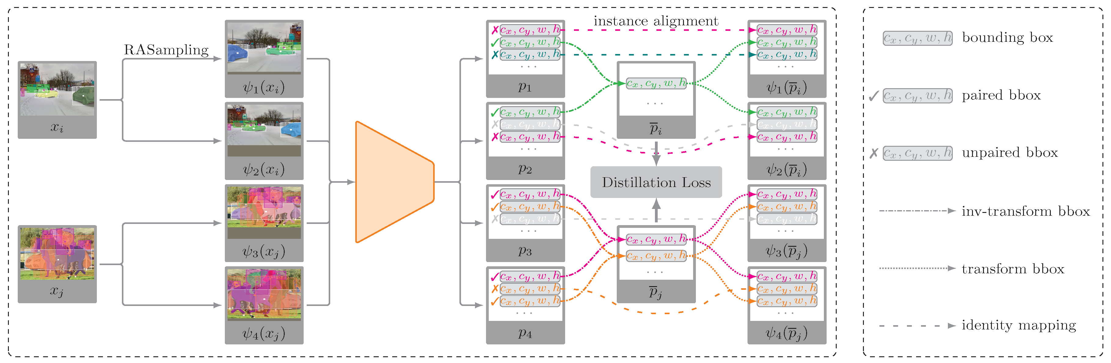
Figure 2.
Test error of ResNet-20 and DenseNet-40 on CIFAR-10 dataset. The model trained with LossTransform effectively gains lower test errors and accelerates the training process.
Figure 2.
Test error of ResNet-20 and DenseNet-40 on CIFAR-10 dataset. The model trained with LossTransform effectively gains lower test errors and accelerates the training process.
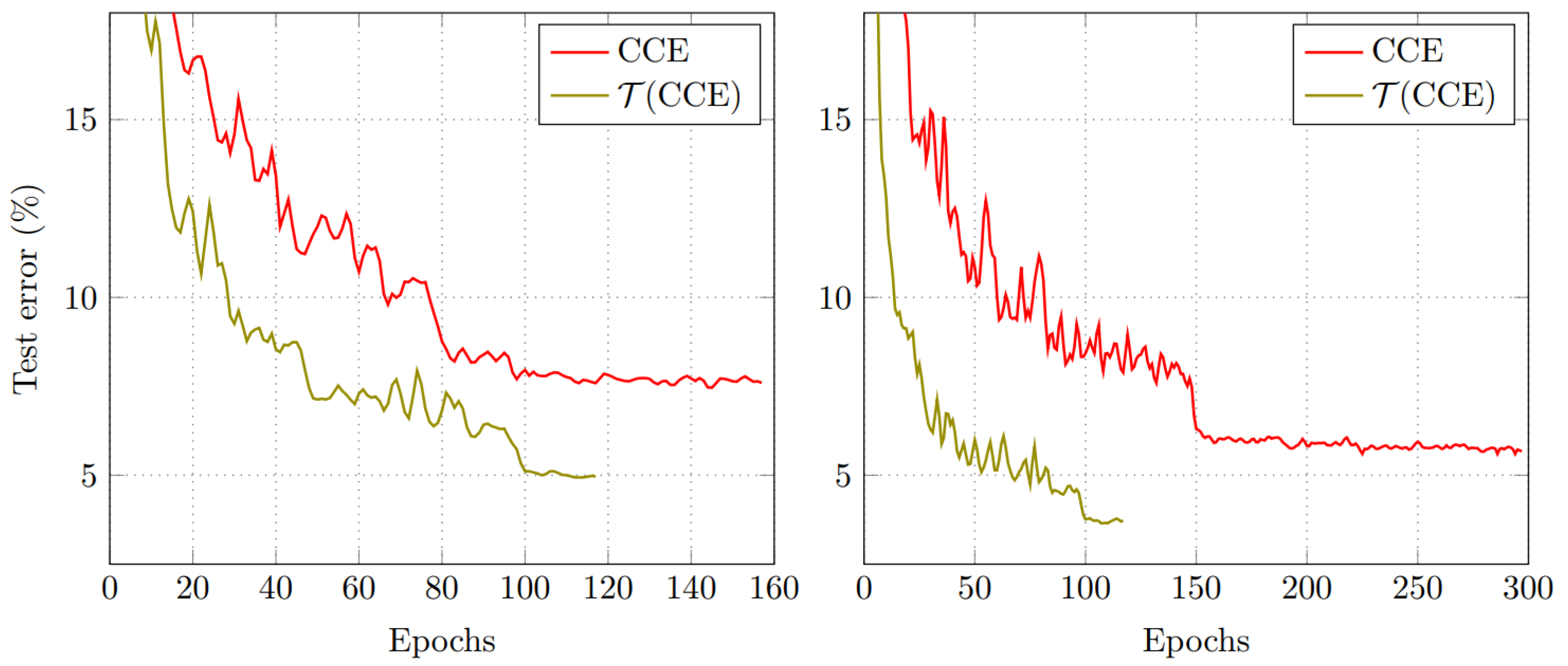
Figure 3.
The predicted probabilities of eight augmented images. The left matrix corresponds to the predicted probabilities of a plain-trained ResNet-20 model. The right matrix corresponds to the predicted probabilities of a LossTransform-trained ResNet-20 model.
Figure 3.
The predicted probabilities of eight augmented images. The left matrix corresponds to the predicted probabilities of a plain-trained ResNet-20 model. The right matrix corresponds to the predicted probabilities of a LossTransform-trained ResNet-20 model.
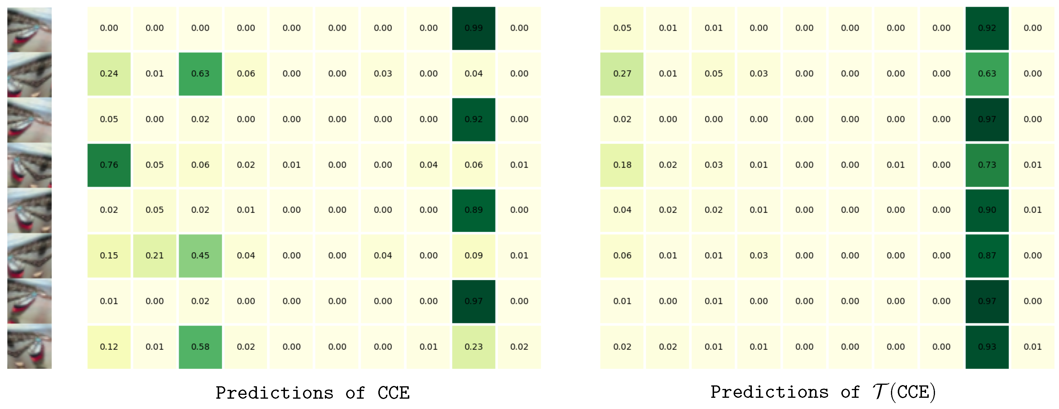
Figure 4.
Left: All networks tend to gain more performance improvement with the growing number of repetitions m. Right: Small models gain more improvement in CIFAR-10@Acc1 and CIFAR-100@Acc5 tests.
Figure 4.
Left: All networks tend to gain more performance improvement with the growing number of repetitions m. Right: Small models gain more improvement in CIFAR-10@Acc1 and CIFAR-100@Acc5 tests.
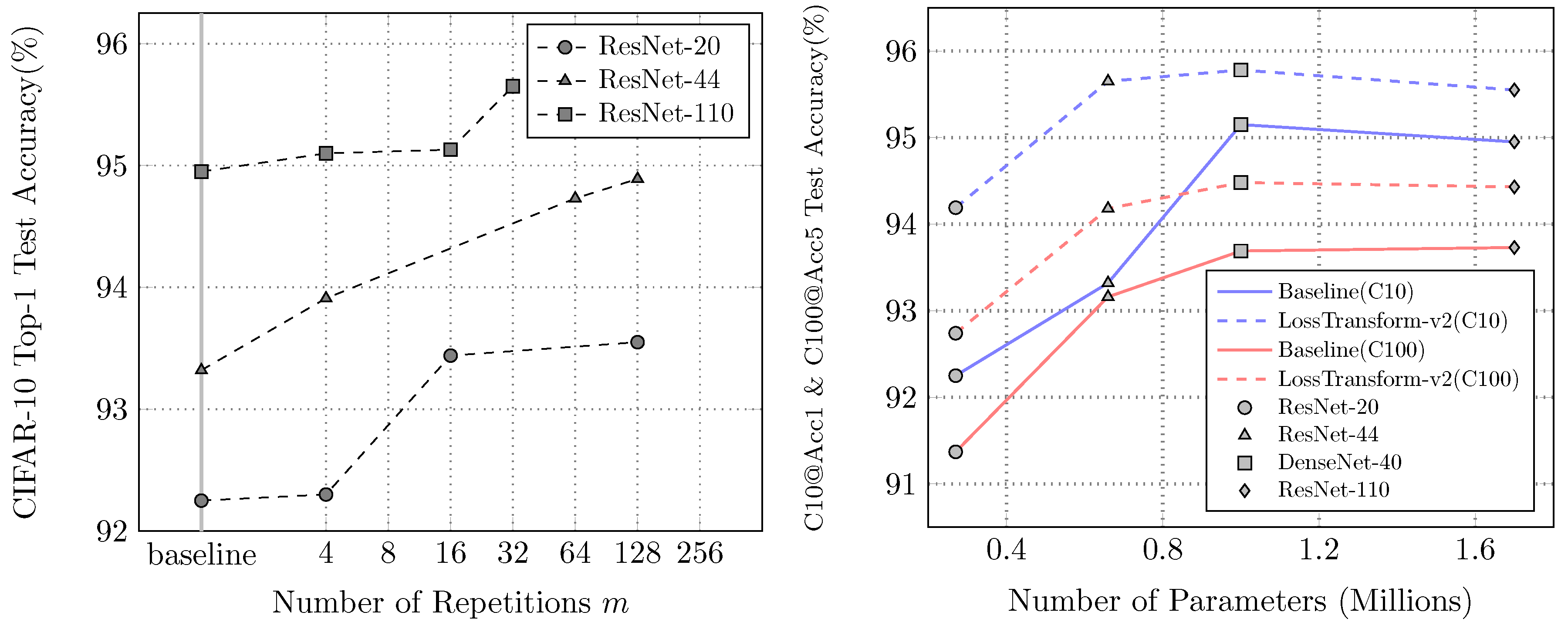

Table 1.
Test error rates (%) of plain/LossTransform-trained models on CIFAR-10. The affine transformation [22] and horizontal flipping schemes are used by default. Cutout [23], CutMix [24] and mixup [25] are optional. The number of repetitions for Repeated Augmentation Sampling is set to 32.
| Model | Cutout | CutMix | mixup | CCE | |
|---|---|---|---|---|---|
| ✗ | ✗ | ✗ | 7.07 | 6.46 | |
| ResNet-20 | ✓ | ✗ | ✗ | 7.23 | 6.70 |
| #params=0.27M | ✗ | ✓ | ✗ | 7.50 | 6.13 |
| ✗ | ✓ | ✓ | 7.70 | 6.27 | |
| ✗ | ✗ | ✗ | 6.32 | 5.73 | |
| ResNet-40 | ✓ | ✗ | ✗ | 6.22 | 5.58 |
| #params=0.66M | ✗ | ✓ | ✗ | 5.99 | 4.47 |
| ✗ | ✓ | ✓ | 7.70 | 4.39 | |
| ✗ | ✗ | ✗ | 6.10 | 5.64 | |
| ResNet-110 | ✓ | ✗ | ✗ | 5.71 | 4.90 |
| #params=1.7M | ✗ | ✓ | ✗ | 5.07 | 4.28 |
| ✗ | ✓ | ✓ | 5.76 | 4.02 |
Table 2.
Test error rates on CIFAR-10 and CIFAR-100 datasets. Comparisons with default CCE (baseline) and Supervised Contrastive Learning (SupCon).
Table 2.
Test error rates on CIFAR-10 and CIFAR-100 datasets. Comparisons with default CCE (baseline) and Supervised Contrastive Learning (SupCon).
| Model | loss function | CIFAR-10 | CIFAR-100 |
|---|---|---|---|
| ResNet-20 #params=0.27M |
CCE | 7.70% | 33.60% |
| SupCon | 6.55% | 31.10% | |
| 6.27% | 28.59% | ||
| ResNet-40 #params=0.66M |
CCE | 6.68% | 29.80% |
| SupCon | 5.23% | 26.48% | |
| 4.39% | 25.34% | ||
| ResNet-110 #params=1.7M |
CCE | 5.76% | 28.45% |
| SupCon | 4.56% | 25.14% | |
| 4.02% | 24.37% | ||
| DenseNet-40 #params=1.0M |
CCE | 5.67% | 27.37% |
| SupCon | 4.52% | 24.90% | |
| 4.35% | 23.55% | ||
| ResNet-50 #params=25.6M |
CCE | 5.0% | 29.7% |
| SimCLR | 6.4% | 29.3% | |
| Max-Margin | 7.6% | 29.5% | |
| SupCon | 4.0% | 23.5% |
Table 3.
Comparison among the pre-trained models and fine-tuned models on the ImageNet-1K validation set.
Table 3.
Comparison among the pre-trained models and fine-tuned models on the ImageNet-1K validation set.
| Model | loss function | Acc@1 | Acc@5 |
|---|---|---|---|
| MobileNet-V2 | CCE | 70.81% | 89.93% |
| 71.26% | 90.48% | ||
| NASNetMobile | CCE | 72.35% | 90.87% |
| 73.14% | 91.54% | ||
| EfficientNet-B0 | CCE | 74.57% | 92.13% |
| 77.09% | 93.61% |
Table 4.
Comparison with the multi-task loss function of Mask R-CNN on PennFudanPed object detection and instance segmentation. Horizontal flipping, random cropping and simple copy-paste data augmentations are used, and all models are trained from scratch. Mask R- is initialized with a MS COCO pre-trained model and fine-tuned on the new dataset.
| Backbone | loss | Detection (%) | Segmentation (%) | ||||
|---|---|---|---|---|---|---|---|
| AP | AP50 | AP75 | AP | AP50 | AP75 | ||
| ConvNeXt-tiny | 65.4 | 96.7 | 82.7 | 60.5 | 91.5 | 79.2 | |
| 65.6 | 96.9 | 83.6 | 63.5 | 94.0 | 81.8 | ||
| DensNet121 | 64.6 | 96.7 | 74.9 | 62.8 | 96.7 | 74.8 | |
| 67.1 | 99.8 | 82.7 | 68.7 | 99.8 | 88.3 | ||
| EfficientNetB4 | 73.8 | 100 | 91.3 | 66.8 | 96.8 | 88.7 | |
| 74.4 | 100 | 91.4 | 69.0 | 100 | 85.6 | ||
| GoogLeNet | 59.6 | 98.9 | 74.0 | 60.1 | 98.9 | 75.8 | |
| 59.4 | 96.6 | 68.7 | 63.1 | 96.1 | 81.6 | ||
| InceptionV3 | 71.0 | 99.7 | 87.0 | 64.6 | 99.5 | 82.2 | |
| 75.0 | 99.8 | 91.5 | 66.9 | 99.8 | 88.8 | ||
| MNASNet1.0 | 61.7 | 94.1 | 78.3 | 56.0 | 94.1 | 65.7 | |
| 65.5 | 96.5 | 81.1 | 61.0 | 93.7 | 83.0 | ||
| ResNet50 | 66.1 | 99.5 | 78.4 | 64.6 | 99.4 | 80.4 | |
| 70.7 | 99.9 | 88.6 | 70.1 | 99.9 | 91.8 | ||
| ShuffleNetV2 | 70.5 | 100 | 83.9 | 62.7 | 96.8 | 81.8 | |
| 72.0 | 99.3 | 90.9 | 64.0 | 96.5 | 85.6 | ||
| WideResNet50 | 69.0 | 100 | 84.5 | 70.8 | 100 | 91.2 | |
| 74.2 | 100 | 90.9 | 71.3 | 100 | 92.2 | ||
| Mask R- | 86.9 | 100 | 96.8 | 80.6 | 100 | 96.8 | |
| 88.2 | 100 | 96.7 | 81.9 | 100 | 96.7 | ||
Table 5.
Comparison among the pre-trained and fine-tuned models on the ImageNet-1K validation set.
| Backbone | Baseline (%) | LossTrans (%) | ||
|---|---|---|---|---|
| Acc@1 | Acc@5 | Acc@1 | Acc@5 | |
| ResNet-50 | 76.130 | 92.862 | 76.206 | 93.138 |
| ResNext-50 | 77.618 | 93.698 | 77.853 | 93.923 |
| MobileNet-V2 | 71.878 | 90.286 | 72.020 | 90.310 |
| EfficientNet-B0 | 77.692 | 93.532 | 77.817 | 93.674 |
| ViT-B16 | 81.072 | 95.318 | 82.019 | 95.326 |
Table 6.
Comparison among the pre-trained and fine-tuned models on MS COCO object detection task. Horizontal flipping data augmentation is used, and all model heads are trained from scratch.
Table 6.
Comparison among the pre-trained and fine-tuned models on MS COCO object detection task. Horizontal flipping data augmentation is used, and all model heads are trained from scratch.
| Model | #Params | loss | Box MAP |
|---|---|---|---|
| Faster R-CNN | 41.8M | 37.0% | |
| ResNet-50 FPN | 37.1% | ||
| Faster R-CNN | 19.4M | 32.8% | |
| MobileNetV3-L FPN | 33.2% | ||
| RetinaNet | 34.0M | 36.4% | |
| ResNet-50 FPN | 36.6% |
Disclaimer/Publisher’s Note: The statements, opinions and data contained in all publications are solely those of the individual author(s) and contributor(s) and not of MDPI and/or the editor(s). MDPI and/or the editor(s) disclaim responsibility for any injury to people or property resulting from any ideas, methods, instructions or products referred to in the content. |
© 2025 by the authors. Licensee MDPI, Basel, Switzerland. This article is an open access article distributed under the terms and conditions of the Creative Commons Attribution (CC BY) license (http://creativecommons.org/licenses/by/4.0/).
Copyright: This open access article is published under a Creative Commons CC BY 4.0 license, which permit the free download, distribution, and reuse, provided that the author and preprint are cited in any reuse.


