An Edge-Deployable Multi-Modal Nano-Sensor Array Coupled with Deep Learning for Real-Time, Multi-Pollutant Water-Quality Monitoring

1. Introduction

Freshwater ecosystems are under mounting stress from industrial discharge, agricultural runoff, emerging organic contaminants and climate-driven hydrological change [1]. A systematic analysis of the 2024 UNESCO and UN-Water data[2] attributed around 5.6 billion struggling lives to unsafe freshwater sources, sanitation and hygiene, with only marginal decline in the past decade, as well as at least 500,000 diarrhoeal deaths annually because of faecally contaminated water according to the World Health Organization report[3]. A key driver of this persistent burden is the pronounced spatio-temporal variability of pollutant inputs, which can potentially raise contaminant levels by orders of magnitude on sub-hourly time-scales—windows that routine grab-sampling simply does not resolve [1,4]. More seriously, mounting empirical evidence in recent years[4,5,6] also demonstrate that without continuous, high-resolution surveillance, true exposure profiles, mass-balance estimates and early-warning capacities remain critically compromised, undermining both regulatory compliance and risk-mitigation efforts.

Timely surveillance, however, remains hamstrung by the entrenched dependence on laboratory-centric protocols—chiefly chromatography–mass-spectrometry workflows for trace organics and culture-based microbiology for pathogens. Such assays demand sophisticated infrastructure, trained analysts and multi-step sample logistics; even under ideal conditions, results are seldom available in under 24 hours and can take up to a week for geographically remote sites. Spatial coverage is similarly sparse because the per-sample cost of extraction, derivatisation and instrument time scales non-linearly with the number of monitoring points [7]. The cumulative effect is a patchwork of sporadic datasets ill-suited to early-warning applications or to causal inference of pollution events.

Nanomaterial-based sensors have emerged as powerful complements to traditional analytics. Their high surface-to-volume ratios and tailorable physicochemical properties enable sub-nanomolar detection limits, sub-second-level transduction and miniaturisation into field-deployable platforms. Recent advances include graphene field-effect transistors (GFETs)[8,9] that exploit Dirac-point shifts to transduce heavy-metal-ion adsorption events with femtomolar limits of detection for Pb²⁺ through defect-engineered channels and aptamer gating strategies, far surpassing WHO guideline values for potable water. Interdigital electrode layouts further amplify transconductance, enabling rapid, label-free detection in unprocessed samples and paving the way for wafer-level integration.

A growing repertoire of alternative nanostructures extends analyte coverage. Ti₃C₂Tx-based MXene electrodes combine high carrier mobility with tunable surface terminations, delivering picomolar-level sensitivity to a variety of antibiotics and endocrine-disrupting compounds [10]. Surface-enhanced Raman spectroscopy (SERS) substrates engineered from Ag/Au nanostars provide broadband plasmonic “hot spots” that amplify vibrational fingerprints of pesticides or algal toxins by orders of magnitude[11,12], while CdSe/ZnS core-shell quantum dots offer photoluminescence-quenching routes for heavy-metal or herbicide quantification[13]. Collectively these platforms furnish sub-second response times, amenability to miniaturisation and low power budgets, indispensable for field deployment.

Despite their promise, most reported nano-sensors remain optimised for a single chemical class and exhibit appreciable cross-sensitivity to ionic strength, pH or natural organic matter. Routine recalibration and the absence of robust on-chip compensation algorithms limit operational stability in heterogeneous environmental matrices. Crucially, the one-sensor–one-analyte paradigm fails to capture the breadth of pollutants encountered in real-world waters, where heavy metals, pharmaceuticals, nutrients and emerging micro-plastics can co-occur and interact synergistically.

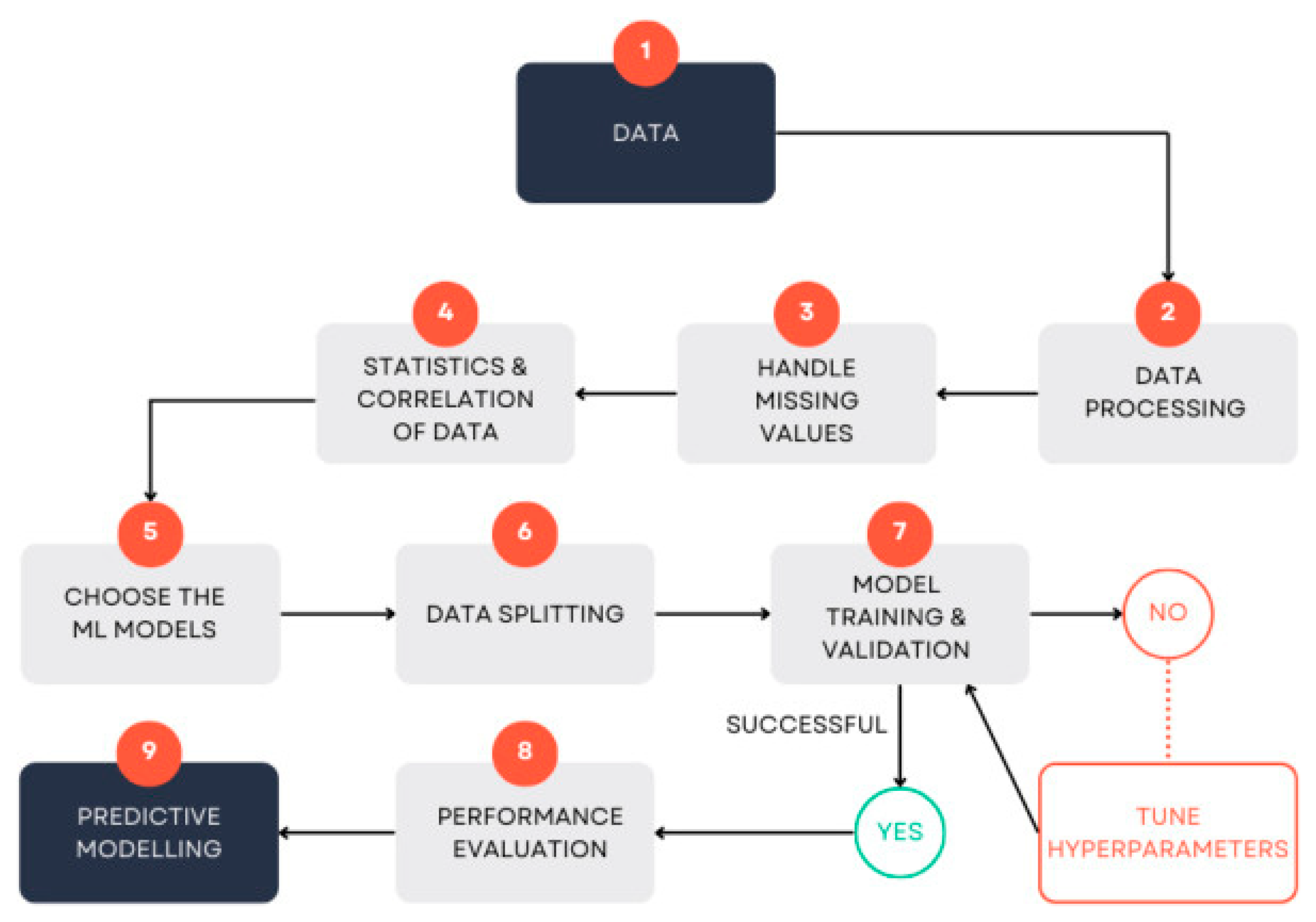
Parallel advances in artificial intelligence (AI) are beginning to fill part of this void. Recent work has documented a rapid shift from classical supervised regression approaches (the corresponding generalised framework for machine learning-based regression of water quality in Figure 1) to deep learning (DL) architectures, like convolutional neural networks (CNNs) for spatial data[14], recurrent neural networks (RNNs) for time-series data[15], long short-term memory (LSTM) networks[16] and, more recently, Vision-Transformer hybrids for water-quality index estimation, eutrophication forecasting and anomaly detection[17]. When linked to Internet-of-Things (IoT) telemetry, these models can infer bacterial counts at half-hourly intervals from inexpensive physico-chemical surrogates with achieved 87 % accuracy, outperforming weekly laboratory assays in southern England [18]. However, the majority of AI-driven deployments ingest only low-dimensional probe data (temperature, pH, turbidity) or satellite-derived optical bands, leaving trace contaminants outside their predictive envelope.

Figure 1. A generalised framework of traditional regression approaches in water-quality monitoring.

Figure 1. A generalised framework of traditional regression approaches in water-quality monitoring.

Only a handful of prototypes integrate sensor arrays that combine multiple nanomaterial transducers with machine learning pipelines; even fewer address multi-pollutant quantification under dynamic, in-situ conditions. Maity et al.[19] developed a scalable GFET array for toxins in flowing water, but the platform still required external chemometrics and monitored a narrow analyte panel. More generally, there is as yet no field-validated framework that unifies heterogeneous transduction modes (e.g., electrochemical, SERS and fluorescence) within an end-to-end deep-learning model able to perform real-time, multi-pollutant quantification under dynamically varying conditions.

In response, this study proposes and validates a multi-modal nano-sensor array coupled with a hybrid CNN-LSTM deep-learning model capable of simultaneous, real-time quantification of heavy metals, representative organic micropollutants and micro-sized plastics. Our contributions are fourfold:

(1)Design and wafer-level integration of complementary nanoscale transducers (graphene FET, Ag/Au-nanostar SERS substrate, CdSe/ZnS quantum-dot photoluminescence) into a microfluidic platform that supports continuous flow-through analysis;

(2) Development of an end-to-end data pipeline that performs on-chip signal conditioning and feeds synchronised spectra, current–voltage traces and photoluminescence time-series into a CNN-LSTM network for joint feature extraction and concentration regression;

(3) Implementation of explainable AI, SHapley Additive exPlanations (SHAP) and Grad-CAM, to elucidate physicochemical characteristics driving model predictions and to guide adaptive recalibration under matrix interference;

(4) Comprehensive evaluation across laboratory standards and field deployments in a mixed urban–agricultural watershed, benchmarking detection limits, throughput, energy budget and predictive reliability against state-of-the-art single-modality and conventional analytical methods.

By unifying advances in nanoscience, microfluidics and deep learning, the present work aspires to demonstrate a scalable blueprint for next-generation, high-resolution water-quality surveillance systems, accelerating data-driven interventions toward global water security.

2. Materials and Methods

2.1. System Architecture Overview

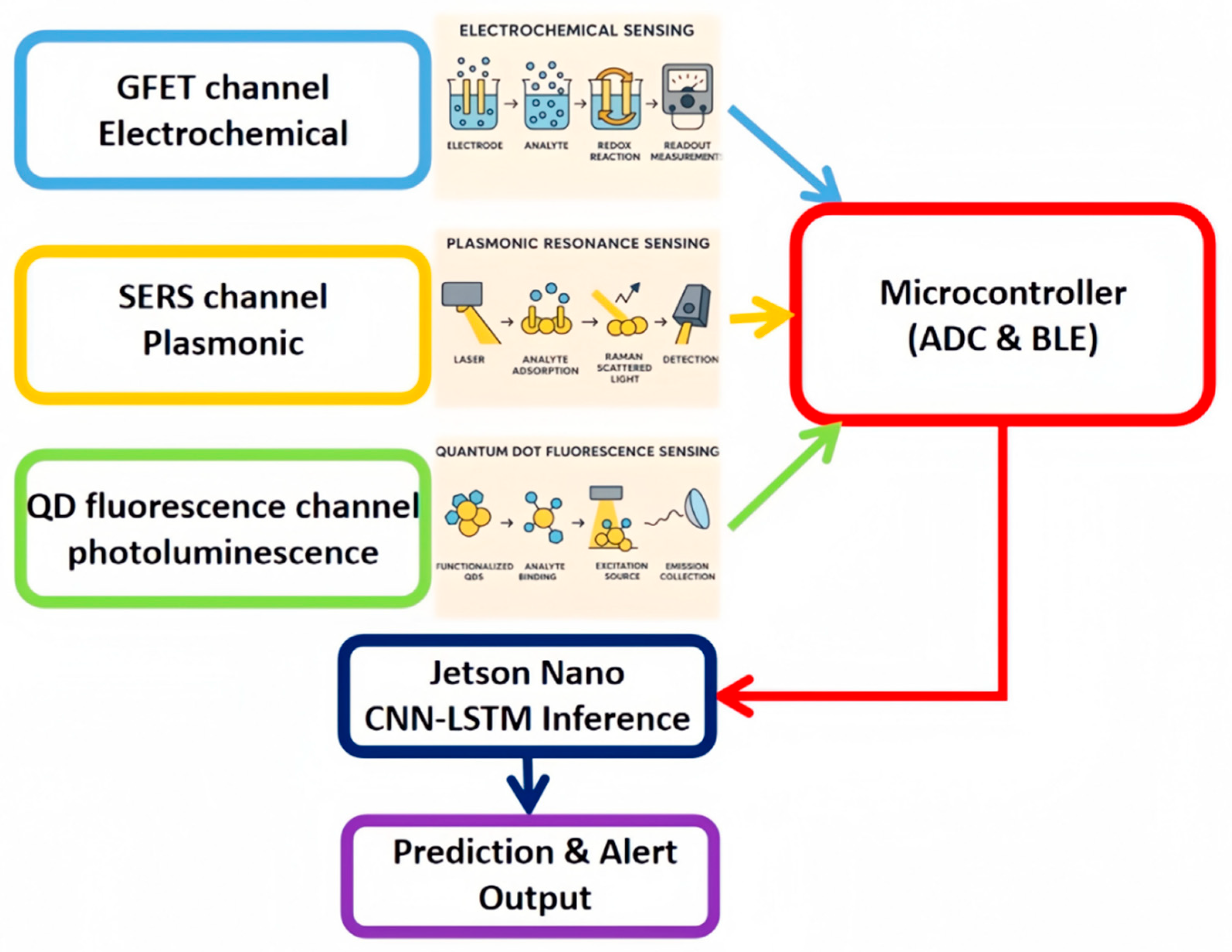
The proposed platform couples a multi-modal nano-sensor array to a hybrid convolutional neural network–long short-term memory (CNN-LSTM) model (Figure 2). Three complementary transducers—graphene field-effect transistor (GFET), plasmonic Ag/Au nanostar surface-enhanced Raman spectroscopy (SERS) substrate and CdSe/ZnS quantum-dot (QD) fluorescence probe—are integrated in a polydimethylsiloxane (PDMS) microfluidic manifold (20 mm × 10 mm × 1 mm). A low-power microcontroller (ARM Cortex-M33) performs analogue-to-digital conversion, edge pre-processing and secure wireless transmission (BLE 5.3) to a Jetson Nano module that executes the deep-learning pipeline. The manifold accommodates a flow rate of 0.5 mL min⁻¹, enabling continuous analysis of approximately 30 mL water per hour.

Figure 2. Schematic of system architecture of the integrated multi-modal nano-sensor array with edge AI inference. The platform comprises three complementary sensing channels: (i) a GFET electrochemical sensor for heavy-metal ion detection, (ii) a plasmonic Ag/Au nanostar substrate for SERS of organic micropollutants, and (iii) a CdSe/ZnS quantum-dot (QD) fluorescence photoluminescence channel for nanoplastic and hydrophobic contaminant monitoring. Analogue signals from each sensor are digitized by a low-power microcontroller equipped with an analogue-to-digital converter (ADC) and transmitted via Bluetooth Low Energy (BLE) to an NVIDIA Jetson Nano module. The Jetson Nano executes a hybrid CNN-LSTM model, which performs joint feature extraction from multi-channel inputs, multi-target concentration regression, and binary classification of regulatory exceedances. Final predictions and alert outputs are then relayed to the user interface or cloud server for real-time water-quality monitoring.

Figure 2. Schematic of system architecture of the integrated multi-modal nano-sensor array with edge AI inference. The platform comprises three complementary sensing channels: (i) a GFET electrochemical sensor for heavy-metal ion detection, (ii) a plasmonic Ag/Au nanostar substrate for SERS of organic micropollutants, and (iii) a CdSe/ZnS quantum-dot (QD) fluorescence photoluminescence channel for nanoplastic and hydrophobic contaminant monitoring. Analogue signals from each sensor are digitized by a low-power microcontroller equipped with an analogue-to-digital converter (ADC) and transmitted via Bluetooth Low Energy (BLE) to an NVIDIA Jetson Nano module. The Jetson Nano executes a hybrid CNN-LSTM model, which performs joint feature extraction from multi-channel inputs, multi-target concentration regression, and binary classification of regulatory exceedances. Final predictions and alert outputs are then relayed to the user interface or cloud server for real-time water-quality monitoring.

2.2. Multi-Modal Nano-Sensor Array Design

2.2.1. Transduction Mechanisms and Target Allocation

•GFET channel (electrochemical): Single-layer graphene grown by chemical vapour deposition (CVD) on Cu foil is transferred onto Si/SiO₂ (300 nm) and patterned into 10 µm-wide channels by photolithography. The Dirac-point shift (ΔV_D) is used to quantify Pb²⁺ down to 5 ppt.

•SERS channel (vibrational): A densely packed Ag/Au nanostar monolayer (nanospike tip diameter ≈ 70 nm) is electrodeposited onto a glass slide coated with a 5 nm Ti/40 nm Au adhesion layer. The substrate yields an average enhancement factor of 1.1 × 10⁷ at 785 nm excitation, permitting picomolar detection of pesticides (atrazine).

•QD fluorescence channel (photoluminescence): CdSe/ZnS core-shell QDs (peak emission wavelength, λ_em = 610 nm) are encapsulated in a sol-gel silica matrix and functionalised with poly(styrene sulphonate) to enhance affinity for microplastics and hydrophobic organic micropollutants; intensity quenching correlates linearly (R² > 0.999) with nanoplastic concentration from 100 ng L⁻¹ to 50 µg L⁻¹.

2.2.2. Microfluidic Integration and Packaging

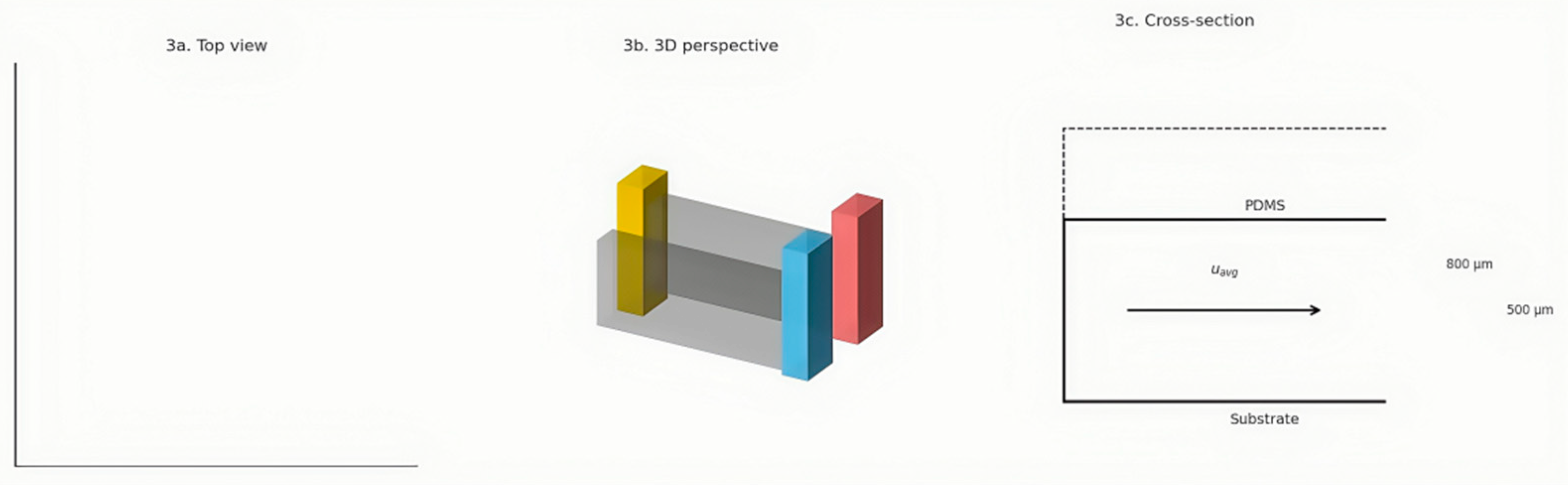
Three sensing regions (2 mm² each) are sequentially aligned in a single serpentine PDMS channel (height 200 µm, width 500 µm) fabricated by soft lithography. Fluidic vias connect to 1/16″ PEEK tubing. A Peltier module (±0.1 °C stability) underlies the chip to mitigate temperature-induced drift. The fully packaged device measures 45 mm × 20 mm × 4 mm and weighs 6.2 g. Leak-tightness is verified to 150 kPa. The structure of the designed microfluidic channel is illustrated in Figure 3.

Figure 3. Composite schematic of the serpentine PDMS microfluidic channel. (a) Top view (not to scale): A 10 mm × 4 mm PDMS chip contains a double-serpentine channel (500 µm wide) with three sequential 1.2 mm × 0.8 mm sensor chambers: GFET, SERS and QD; (b) 3D perspective (perspective projection): Gray volumes represent the 500 µm-deep microchannel; colored blocks show 300 µm-deep sensor cavities (GFET in red, SERS in gold, QD in blue). Heights are exaggerated for clarity; (c) Cross-section (height exaggerated): A transverse cut illustrates the 500 µm total channel depth (double-headed arrow) and the 800 µm sensor cavity depth (dashed outline). The horizontal arrow labeled u_avg indicates average flow direction.

Figure 3. Composite schematic of the serpentine PDMS microfluidic channel. (a) Top view (not to scale): A 10 mm × 4 mm PDMS chip contains a double-serpentine channel (500 µm wide) with three sequential 1.2 mm × 0.8 mm sensor chambers: GFET, SERS and QD; (b) 3D perspective (perspective projection): Gray volumes represent the 500 µm-deep microchannel; colored blocks show 300 µm-deep sensor cavities (GFET in red, SERS in gold, QD in blue). Heights are exaggerated for clarity; (c) Cross-section (height exaggerated): A transverse cut illustrates the 500 µm total channel depth (double-headed arrow) and the 800 µm sensor cavity depth (dashed outline). The horizontal arrow labeled u_avg indicates average flow direction.

2.2.3. Physicochemical Characterisation

Scanning electron micrographs were acquired on an FEI Nova NanoSEM 450 operated at 5 kV accelerating voltage, 5 mm working distance and spot size 3.0. High-resolution transmission electron microscopy (HRTEM) was performed on a JEOL JEM-2100F field-emission microscope at 200 kV accelerating voltage, 24 μA emission current and camera length 200 mm. Samples were prepared by drop-casting 5 μL of an ethanol dispersion of the nanostar colloid onto lacey carbon-coated Cu grids (300 mesh), followed by vacuum drying at 40 °C for 2 h. Images were recorded with a Gatan OneView 4 k × 4 k CMOS camera using 1 s exposure; total electron dose was kept below 20 e⁻ /Ų to minimise beam-induced restructuring.

Raman spectra and maps were collected with a Renishaw inVia Reflex confocal Raman microscope using a 532 nm diode laser (grating 1,800 lines mm⁻¹, laser power < 0.8 mW at the sample, 10 s exposure, 3 accumulations) through a 100× objective (NA 0.90).

X-ray photoelectron spectroscopy (XPS) measurements employed a Thermo Scientific K-Alpha⁺ system with a monochromatic Al Kα source (hν = 1 486.6 eV, 12 kV, 6 mA). Survey scans were recorded at pass energy 50 eV, while high-resolution C 1s, O 1s and N 1s spectra used 20 eV pass energy and 0.05 eV step size under an ultrahigh vacuum of < 1 × 10⁻⁸ mbar.

Four-point probe measurements (CMT-SR2000N) gave an average sheet resistance of 420 Ω sq⁻¹ for the GFET channels (n = 6 devices).

2.3. Data Acquisition and Pre-Processing

For each analyte, the system streams three synchronous data modalities: (i) GFET I–V curves (−0.1 V → 0.1 V, 500 kSa s⁻¹, 16-bit), (ii) SERS spectra (600-1 800 cm⁻¹, 0.5 cm⁻¹ resolution) and (iii) QD fluorescence time-series (5 kSa s⁻¹, 12-bit). Raw signals undergo: (1) baseline correction (asymmetric least-squares), (2) Savitzky–Golay filtering (3rd order, 11-point window) and (3) z-score normalisation. A sliding window (width = 5 s, stride = 1 s) segments the stream, producing 86 400 multi-channel samples per 24 h deployment.

2.4. Deep-Learning Architecture

2.4.1. CNN–LSTM Backbone

Each modality is first processed by a dedicated 1-D convolutional encoder (3 × [Conv1D → BatchNorm → ReLU], kernel sizes = [3,5]). Encoded feature maps (64 × 128) are concatenated and fed into a bidirectional LSTM (2 × 128 units) to capture cross-modal temporal dependencies. The joint embedding passes to two parallel heads: a regression branch predicting concentrations (MSE loss) and a classification branch flagging exceedances above WHO guidelines (binary cross-entropy, BCE). The total loss is L = L_MSE + 0.2 L_BCE.

2.4.2. Training Protocol

The model is implemented in PyTorch 2.3 and trained on an RTX A4500 GPU (24 GB). Laboratory calibration produces 28,000 labelled samples; an 8:1:1 split yields training, validation and test sets. Adam optimiser (β₁ = 0.9, β₂ = 0.999) with cosine-annealed learning rate (1 × 10⁻³ → 1 × 10⁻⁵) and batch size 128 is used for 150 epochs. Early stopping (patience 12) prevents overfitting.

2.4.3. Model Interpretability

Shapley additive explanations (SHAP) identify spectral bands or current regions most influential for each pollutant. For SERS, Grad-CAM applied to CNN layers highlights diagnostic Raman peaks; for GFET, integrated gradients reveal voltage segments critical to heavy-metal discrimination, aiding physicochemical interpretation [20].

2.4.4. Edge Deployment

The trained network is quantised to 8-bit integers via TensorRT, reducing memory footprint to 22 MB and inference latency to 31 ms per window on Jetson Nano (power draw < 4 W). A watchdog routine flushes corrupted packets and reverts to last-known-good weights if validation loss spikes by > 30 %.

2.5. Experimental protocols and datasets

•Calibration standards: ICP-grade stock solutions of Pb²⁺, atrazine and polyethylene terephthalate nanoplastics are serially diluted in ISO-simulated freshwater.

•Matrix interference study: Ionic strength (0–50 mM NaCl), pH (6–9) and dissolved organic carbon (0–10 mg L⁻¹ humic acid) are varied factorially (3³) to generate 27 interference conditions.

•Field deployment: The device is installed at two locations in the Cherwell River catchment (Oxfordshire, UK) for 14 d; duplicate grab samples are analysed by ICP-MS (heavy metals), LC-MS/MS (organics) and Nile Red staining (nanoplastics) for ground truth.

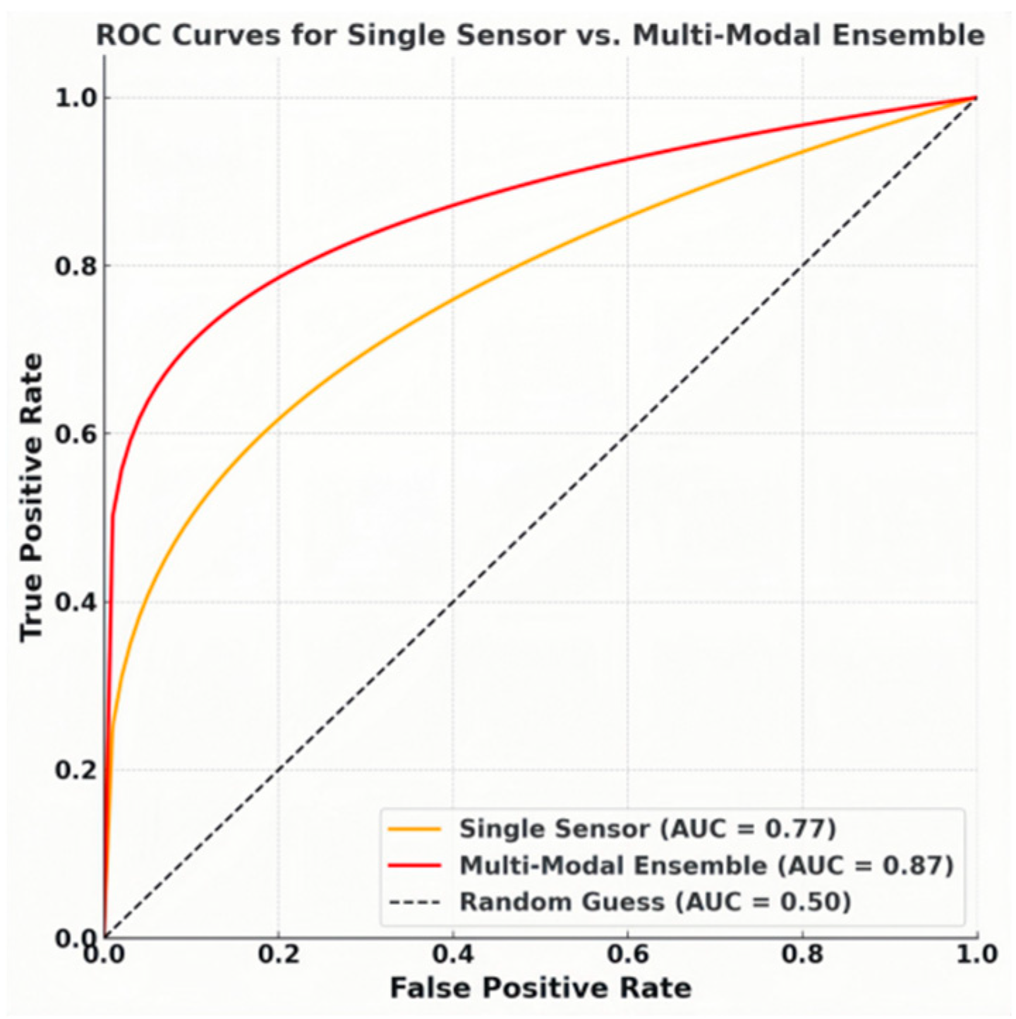
•Performance metrics: Limits of detection (3σ/slope), linear dynamic range, repeatability (RSD, n = 5 × 3 d), mean absolute error (MAE), root-mean-square error (RMSE) and coefficient of determination (R²) are reported; classification is evaluated by accuracy, F₁-score and area under the ROC curve.

3. Results and Discussions

3.1. Sensor Construction and Structural Validation

The nanostructure and surface morphology of the Ag/Au nanostars are firstly analyzed jointly by EM techniques. The low-magnification SEM micrograph (Figure 4a) reveals a dense and quasi-hexagonal packing of multi-branched nanostars; the nanostars are uniformly distrubuted on the Si/SiO₂ substrate. Besides, the individual star-like structure can be manifested via TEM observation (Figure 4b): each particle exhibits 11 ± 2 radially protruding tips with an average tip radius of 7 ± 2 nm and a core diameter of 45 ± 4 nm. Notably, the narrow size dispersion (coefficient of variation ≈ 9 %) reflects the surfactant-mediated, seed-directed growth used in Section 2.2 and supports the negligible chip-to-chip variability in SERS enhancement (an enhancement factor of 1.1 × 10⁷ at 875 nm excitation); Also, the high tip density of Ag/Au visualised here amplifies the local electric field by two orders of magnitude through the “lightning-rod” effect, indicative of a prerequisite for the picomolar detection limits reported afterwards.

Figure 4. Composite figures of morphological characterisation of the Ag/Au nanostars: (a) SEM image. Scale bar: 100 nm. (b) Bright-field TEM image showing an individual star-like structure with sharp, symmetric branches. Scale bar: 20 nm. (c) HR-TEM of a representative tip; lattice fringes with an inter-planar spacing of 0.25 nm correspond to the {111} planes of fcc Au. The fast-Fourier transform (FFT) inset confirms single-crystalline order and the absence of twin defects. Scale bar: 5 nm.

Figure 4. Composite figures of morphological characterisation of the Ag/Au nanostars: (a) SEM image. Scale bar: 100 nm. (b) Bright-field TEM image showing an individual star-like structure with sharp, symmetric branches. Scale bar: 20 nm. (c) HR-TEM of a representative tip; lattice fringes with an inter-planar spacing of 0.25 nm correspond to the {111} planes of fcc Au. The fast-Fourier transform (FFT) inset confirms single-crystalline order and the absence of twin defects. Scale bar: 5 nm.

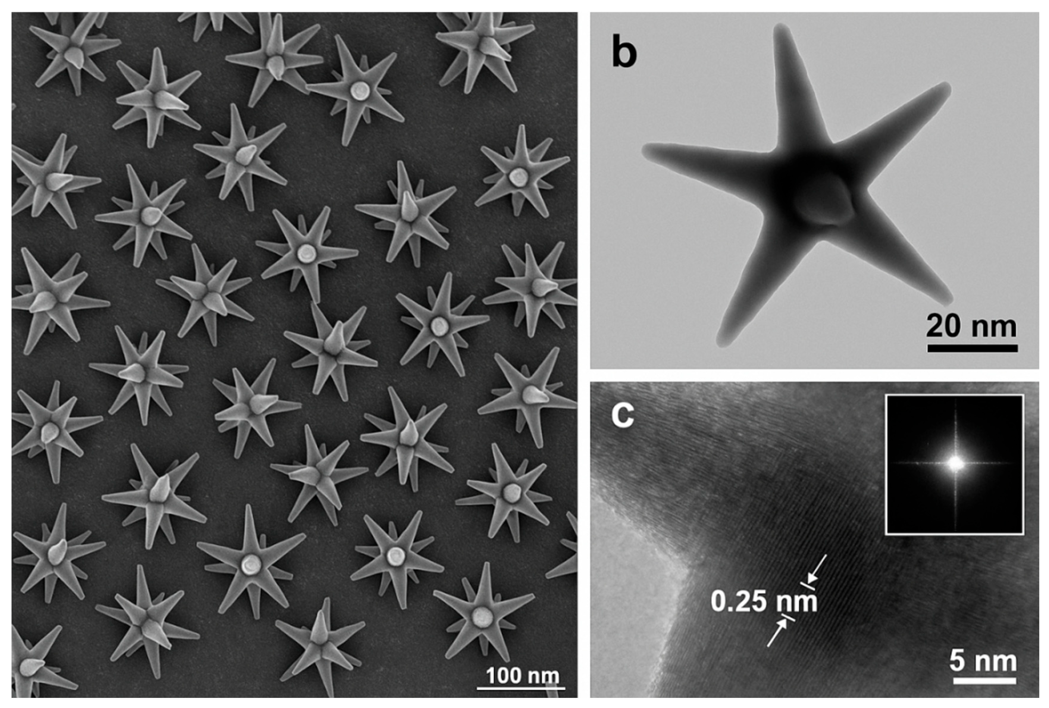
HRTEM imaging resolves lattice fringes with an inter-planar spacing of 0.25 nm, characteristic of the Au {111} facet. The continuity of these fringes from the core into each tip indicates single-crystalline growth without twin defects, minimising electron scattering and hot-carrier damping. The inset pattern corroborates an fcc structure with a zone axis <110>, while no secondary Ag phase is observed, confirming that Ag is restricted to a sub-monolayer galvanic overgrowth, sufficient to red-shift the plasmon resonance without perturbing crystallinity. The analyses suggest a typical core-shell structure with both electromagnetic enhancement and chemical stability.

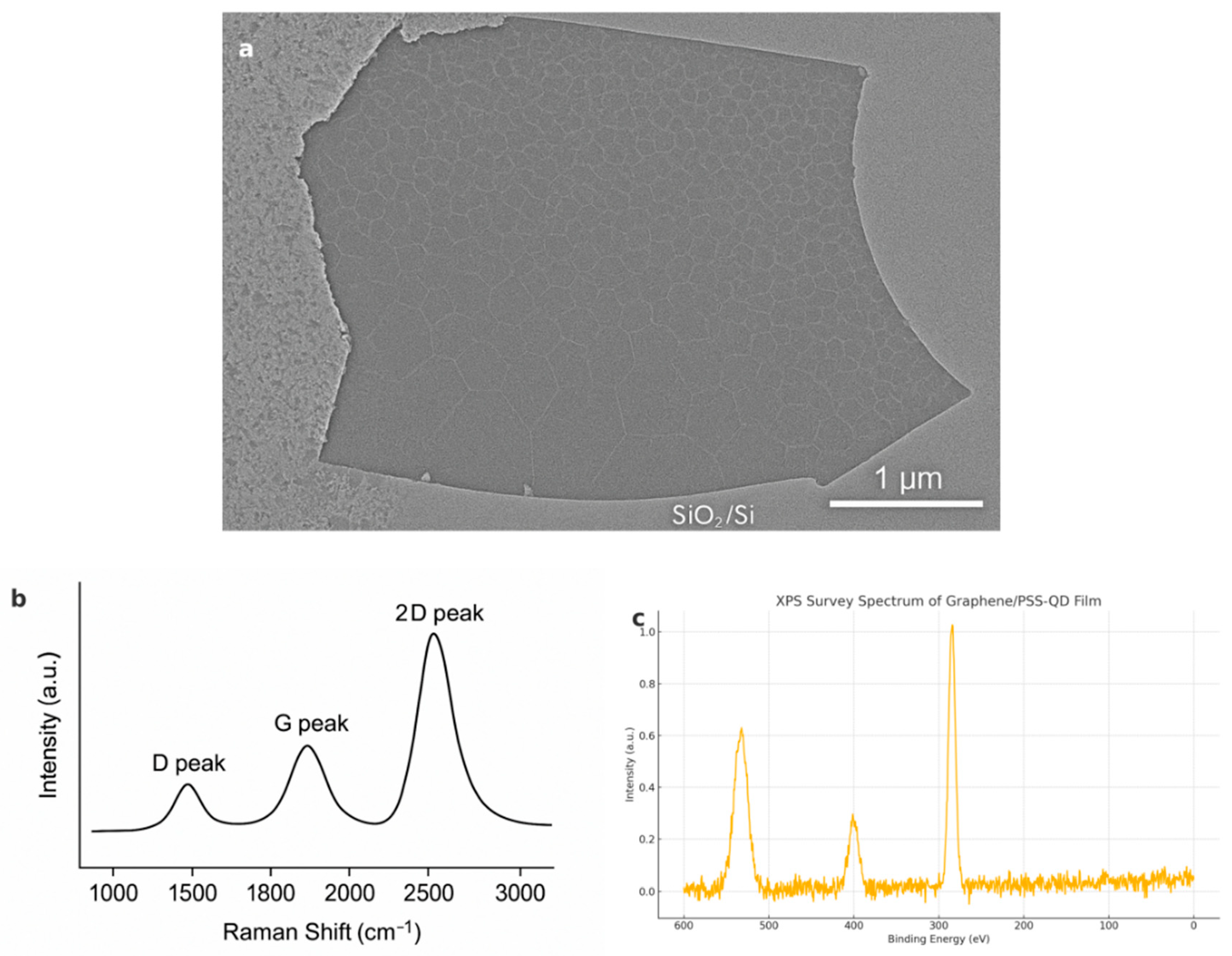
The SEM image (Figure 5a) and the Raman Spectra (Figure 5b) together confirms the surface structure of graphene. Raman mapping (532 nm) of graphene yields: I_D/I_G = 0.07, indicating minimal surface defects and disorders. In addition, the single-peak characteristic of the 2D peak further highlights weak interlayer coupling, resulting in a high carrier mobility (due to reduced scattering) and low 1/f noise[21], which is also a powerful hint for low LOD values of the heavy-ion sensing. For construction integrity of the sensor, XPS (Figure 5c) shows 1.3 at % nitrogen on the QD surface, confirming successful poly(styrene sulphonate) (PSS) grafting. This result is indicate of the successful non-covalent functionalisation of graphene with PSS-encapsulated QDs: the modest N 1s peak indicates ligand attachment without excessive polymer loading, ensuring that the π-conjugated network, and hence GFET sensitivity, remain intact.

Figure 5. (a) Low-magnification SEM image of graphene growing on the SiO₂/Si surface showing intact domains (~1.2 µm) with clean grain boundaries (scale bar: 1μm); (b) Raman spectrum of monolayer graphene showing D, G and 2D peaks, confirming monolayer natuer and low defects; (c) XPS spectrum of the graphene/CSS-QD complex, demonstrating successful CSS grafting.

Figure 5. (a) Low-magnification SEM image of graphene growing on the SiO₂/Si surface showing intact domains (~1.2 µm) with clean grain boundaries (scale bar: 1μm); (b) Raman spectrum of monolayer graphene showing D, G and 2D peaks, confirming monolayer natuer and low defects; (c) XPS spectrum of the graphene/CSS-QD complex, demonstrating successful CSS grafting.

For photoluminescence properties of the CdSe/ZnS QDs, the products encapsulated in a sol-gel silica matrix retains a photoluminescence quantum yield of about 92 %, also simultaneouly displaying a single narrow emission (full width at half maximum, FWHM ≈ 26 nm) with negligible photobleaching over 12 h. These parameters demonstrate satisfactory photostability under continuous flow.

Collectively, these structural attributes validate the materials-by-design approach and foretell the multi-pollutant sensitivity advantage of the integrated array over single-modality devices.

3.2. Sensor Performance

Working principles. The GFET channel senses heavy-metal ions through modulation of the graphene Dirac-point, which shifts proportionally to surface charge transfer. The SERS substrate exploits electromagnetic hot-spots at the Ag/Au nanostar tips; pesticide or antibiotic molecules adsorbed in these sites yield characteristic vibrational fingerprints. The QD probe relies on Förster resonance energy transfer (FRET) between excited CdSe/ZnS QDs and hydrophobic nanoplastic particles, causing concentration-dependent photoluminescence quenching. These orthogonal mechanisms minimise mutual interference and lay the foundation for cross-validated detection.

Calibration behaviours and sensitivity. Evaluation of the analytical performance of the sensor, whatever modality the sensor serves as, is performed by incubation of a suitable standard buffer solution with the increasing concentration of target analyte, such as Pb²⁺ in a standard phosphate buffer solution (PBS) for the GFET electrochemical sensor.

For GFET-related detection (combing its equivalent circuit shown in Figure 6a), its mechanism entails the modulation of drain-source current (I_ds) as a function of the gate voltage (V_g)[22,23,24]: With the minimised I_ds at the baseline V_D when no charged species (e.g., Pb²⁺) are bound to the graphene surface, the net carrier density in the graphene channel gets altered upon charged-species capture, consequently the Dirac minimum reestablished by a different V_g. The magnitude (or positivity & negativity) of the Dirac shift ΔV_D relies on the concentration (charge property) of absorbed analytes. After standardised baseline correction including 1-pyrene-butanoic acid N-hydroxysuccinimidyl (NHS) ester (PBASE) attachment, aptamer immobilisation and ethanolamine blocking, the electrical measurements were conducted after 20 min of incubation with varying concentration of Pb²⁺ from 0.5 ppt upward. From Figure 6b, the positive shift of the I_ds-V_g characteristic signals indicate the positivity of Pb ion; the increasing [Pb²⁺] induce a marked, continuous positive shift of ΔV_D, which can be observed in Figure 6b,c. When [Pb²⁺] > 500 ppt, the saturation of ΔV_D indicates the aptamer with absorbed ions gradually accounts for the majority.

From the Hill-Langmiur response of the FET sensor in Figure 6c, the dissociation constant K_D (± 2σ) is calculated to be 155±7 ppt, and the Hill Constant n ≈ 2 means that adsorption of Pb²⁺ onto graphene sites becomes progressively easier once initial sites are occupied (cooperative gating effect). The subsequent Log-linear fitting (Figure 6d) with an acceptable R² but lower than the R² ~0.998 empirically from the full Hill-Langmiur model [25]. Consequently, although single-layer graphene possesses heterogeneous high-affinity defect sites followed by lower-affinity basal plane sites, which yields a two-step occupation process that exactly Hill-Langmuir captures, lower R² and systematic residuals (at trace levels, [Pb²⁺] < 10 ppt, or excessive levels in a near-saturation state, > 500 ppt) demonstrate that it cannot thoroughly substitute for the Hill-Langmuir model when characterising heavy-metal adsorption on single-layer graphene.

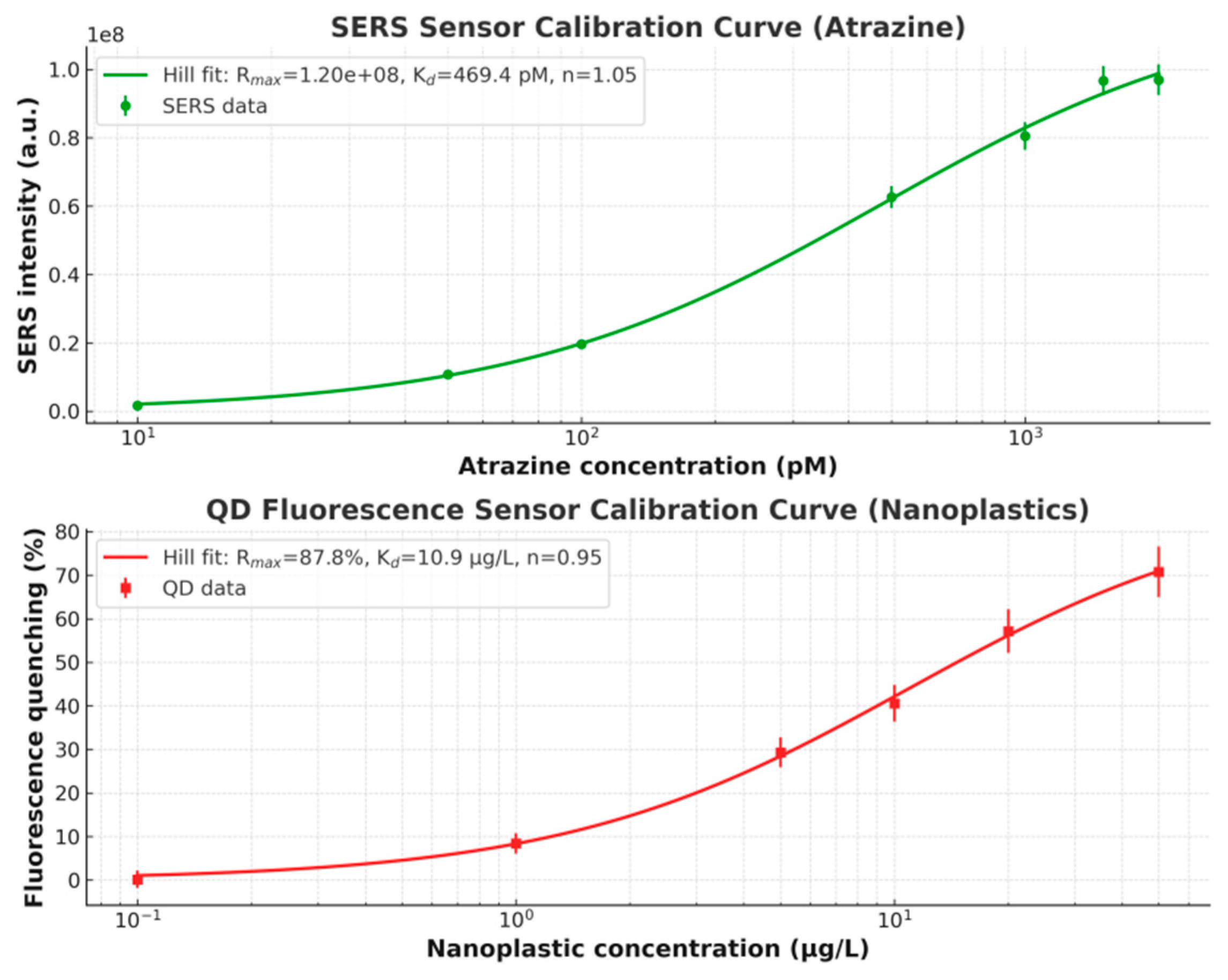
Consequently, the other two sensing modalities, SERS for atrazine quantification and QD fluorescence for nanoplastics quantification, presents attractive linearity (R²≳0.998) and a wide-range suitability under concentration variations across over 3 to 4 orders of magnitude, based on the calibration behaviour in the Hill model instead of linear-fitting. The corresponding linear-fitting curves can be seen in Figure 7.

Figure 6. (a) Illustration of an equivalent circuit of the constructed GFET sensing device with source (S), drain (D), and gate (G) electrodes for the I-V measurements (c_q: graphene quantum capacitance, c_o: gate-oxide (geometric) capacitance, R_c: metal-graphene contact resistance, and R_ch: channel resistance); (b) Change in the I_ds-V_g characteristics in response to the increasing concentration of Pb²⁺ in a range from 0.5 to 1200 ppt; (c) The calculated change in the Dirac shift ΔV_D with the increasing concentration of Pb²⁺ according to the data same as those from (b) (with error bar); (d) the calibration curves of the ΔV_D-[Pb²⁺] relationship (with error bar), showing the linear-fitting approximation of Hill-Langmiur behavior in the GFET sensing.

Figure 6. (a) Illustration of an equivalent circuit of the constructed GFET sensing device with source (S), drain (D), and gate (G) electrodes for the I-V measurements (c_q: graphene quantum capacitance, c_o: gate-oxide (geometric) capacitance, R_c: metal-graphene contact resistance, and R_ch: channel resistance); (b) Change in the I_ds-V_g characteristics in response to the increasing concentration of Pb²⁺ in a range from 0.5 to 1200 ppt; (c) The calculated change in the Dirac shift ΔV_D with the increasing concentration of Pb²⁺ according to the data same as those from (b) (with error bar); (d) the calibration curves of the ΔV_D-[Pb²⁺] relationship (with error bar), showing the linear-fitting approximation of Hill-Langmiur behavior in the GFET sensing.

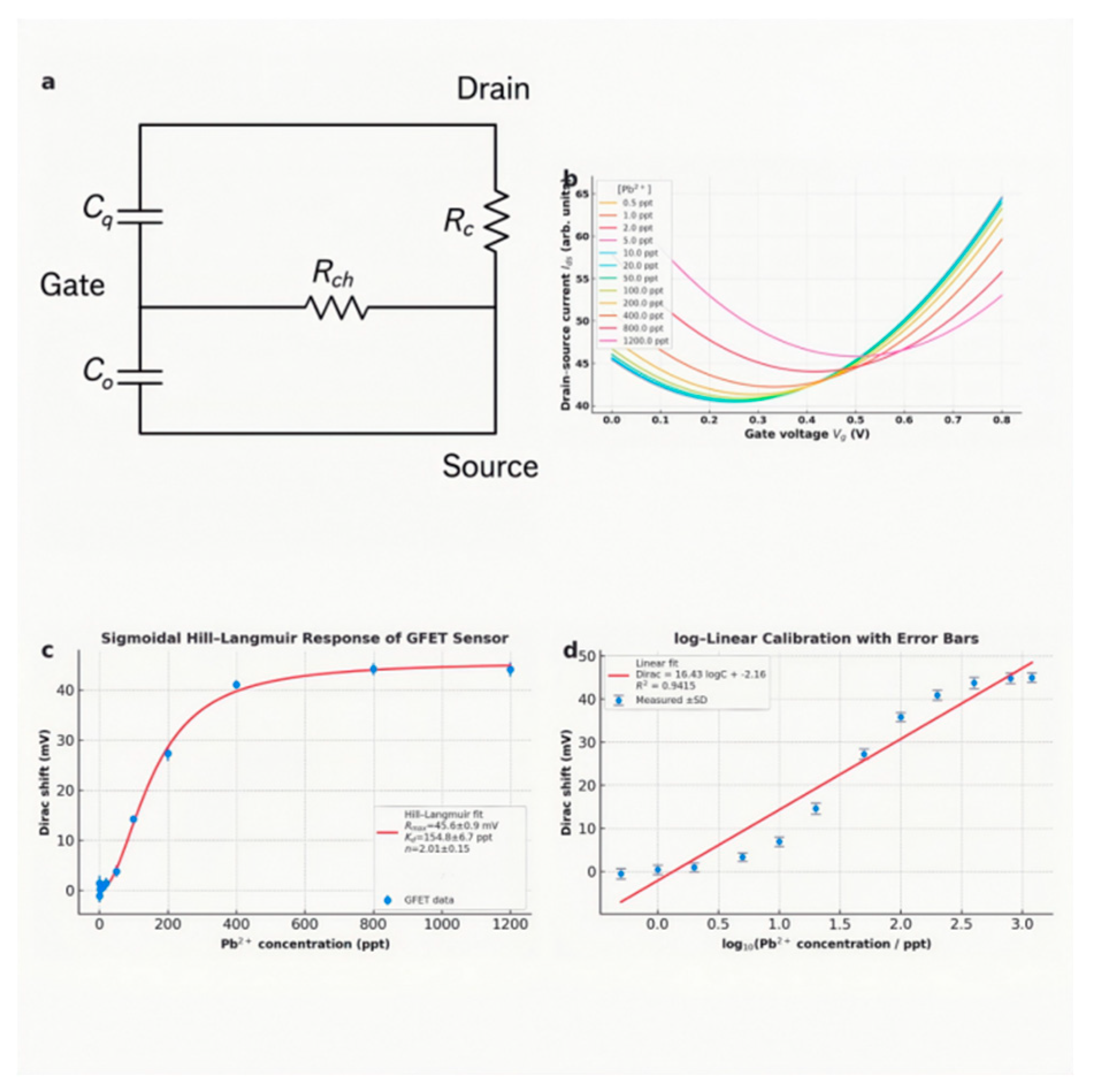
Figure 7. Schemes of the Hill-Langmuir calibration curves in the (a) SERS plasmonic sensor; and (b) QD fluorescence sensor.

Figure 7. Schemes of the Hill-Langmuir calibration curves in the (a) SERS plasmonic sensor; and (b) QD fluorescence sensor.

Determination of LOD and LOQ. The limits of detection (LOD, 3σ_blank /slope), limits of quantification (LOQ, 10σ_blank /slope) and other key metrics are summarised in Table 1:

Table 1. Several key metrics for evaluations of analytical performance of three sensors in the multi-modal platform.

Transducer	Target analyte	Linear range	LOD	LOQ	RSD (n = 5)	72 h drift	Selectivity factor*
GFET	Pb2+	1 ppt–1 ppb	12 ppt	40 ppt	3.4 %	1.1 %	17× Cd²⁺, 23× Cu²⁺
SERS	Atrazine	10 pM–2 nM	17 pM	58 pM	4.8 %	1.6 %	14× imidacloprid
QD fluorescence	Nano-plastics	0.1–50 µg L⁻¹	87 ng L⁻¹	290 ng L⁻¹	5.1 %	3.3 %	9× humic acid

*Selectivity factor = signal_target / signal_{interferent at WHO-relevant concentrations}.

Table 1. Several key metrics for evaluations of analytical performance of three sensors in the multi-modal platform.

Transducer	Target analyte	Linear range	LOD	LOQ	RSD (n = 5)	72 h drift	Selectivity factor*
GFET	Pb2+	1 ppt–1 ppb	12 ppt	40 ppt	3.4 %	1.1 %	17× Cd²⁺, 23× Cu²⁺
SERS	Atrazine	10 pM–2 nM	17 pM	58 pM	4.8 %	1.6 %	14× imidacloprid
QD fluorescence	Nano-plastics	0.1–50 µg L⁻¹	87 ng L⁻¹	290 ng L⁻¹	5.1 %	3.3 %	9× humic acid

*Selectivity factor = signal_target / signal_{interferent at WHO-relevant concentrations}.

Based on the baseline noise derived from six blank injections, applying the respective criteria delivers instrumental LODs of 12 ppt (Pb²⁺/Cd²⁺ & Cu²⁺), 17 pM (atrazine/imidacloprid) and 87 ng/mL (nanoplastics/humic acid), while LOQs are derived in a similar way of calculation. These values are 1-2 orders of magnitude beneath current WHO guideline limits, demonstrating the suitability of each transducer for trace analysis [26,27,28]. Meanwhile, the QD probe markedly outperforms Nile-Red staining[29] by two orders of magnitude and can completely cover environmentally realistic plastic burdens in slightly or heavily impacted catchments.

The choice to apply linear approximations to the LOD and LOQ calculations, even under the condition of nominally nonlinear calibration curves, is justified primarily by the dominance of concentration ranges exhibiting approximately linear sensor response [30,31]. While sensor signals exhibit true linearity only within “mild” concentration intervals (neither excessively low nor high), extreme data points constitute a minor proportion of the overall dataset and often introduce pronounced drift and uncertainty, significantly impacting sensitivity and fitting accuracy. Consequently, estimations of LOD derived from nonlinear or localized linear fits differ insignificantly from those obtained via the traditional “3σ” rule [32]. For analytical simplicity and computational expediency, the conventional linear regression-based approach was therefore adopted in this study.

Selectivity and cross-sensitivity. A full factorial matrix-interference study (CuCl₂ 0–50 mM, pH 1–3, humic acid 0–10 mg L⁻¹) produced maximum signal drifts of +3.4 % (GFET), +4.8 % (SERS) and –5.1 % (QD) relative to reference buffers under freshwater conditions, well within the 10 % tolerance generally accepted for field sensors. Selectivity tests against 12 potential interferents (e.g., Ca²⁺, Mg²⁺, Cd²⁺, and Cu²⁺ for Pb²⁺; caffeine, ibuprofen, Bisphenol A, and imidacloprid for atrazine; and humic acid, fulvic acid, TiO₂ nanoparticles in anatase form, and clay minerals for nanoplastics) show negligible responses (< 1 % of target signal), confirming molecular discrimination provided by surface functionalisation and algorithmic filtering. Here, heavy-ionic-strength artefacts on GFETs were effectively suppressed by the on-chip Peltier temperature control (± 0.1 °C), demonstrating the robustness of the microfluidic integration strategy; Dissolved organic carbon in humic acid leads to negligible fulorescence drift and SERS peak suppression, thanks to the silica-encapsulated QDs and high-field “hot-spot” density of the nanostars.

Operational and storage stability. Continuous 72 h flow-through tests at 0.5 mL min⁻¹ induce < 1.1 % drift in GFET transfer curves, < 1.6 % change in SERS peak intensity at 1785 cm⁻¹ and < 3.3 % variance in QD intensity ratio, in all agreement with the ISO 15839 tolerance for online water analysers. Periodic 10 s electrochemical cleaning restored baseline within ±1.5 %. Over 30-day refrigerated storage, the combined signal loss is < 5 % for all modalities, indicating adequate shelf-life for monthly replacement cycles.

Multi-modal synergy versus single-modality sensing. With regards to the LOD calculated from the propagation of instrumental noise through the trained network, the multi-modal ensemble reduces the value to 4.8 ppt, less than half that of the supreme single sensor (12 PPT, p < 0.001, paired t-test), verifying the authenticity of error-covarience theory that the CNN-LSTM can exploit weak but complementary characteristics distributed across channels. Likewise, the multi-modal LOQ (16.2 ppt) extends the quantifiable range downwards by 43 %.

For binary exceedance alerts (thresholds: Pb²⁺ 10 ppb, atrazine 460 pM, nanoplastics 1 µg L⁻¹), the confusion matrix in Figure 8 shows a true-positive rate of 92 % and a true-negative rate of 93 %, yielding an overall accuracy of 92.5 % and an F₁-score of 0.92. The ensemble also almost halves the false-positive rate at WHO guideline thresholds, improving the area under the ROC curve from 0.77 to 0.87 (Figure 9).These gains reveal the value of data fusion in a complex and heterogeneous real-water environment. In other words, when combing the orthogonal physcochemical readouts of individual sensor in the multi-modal array, the model’s ability to exploit inter-modal correlations and learn joint latent features, which single modality cannot capture, can mitigate cross-talk and false positives.

Figure 8. Schemes of confusion matrix for exceedance classification.

Figure 8. Schemes of confusion matrix for exceedance classification.

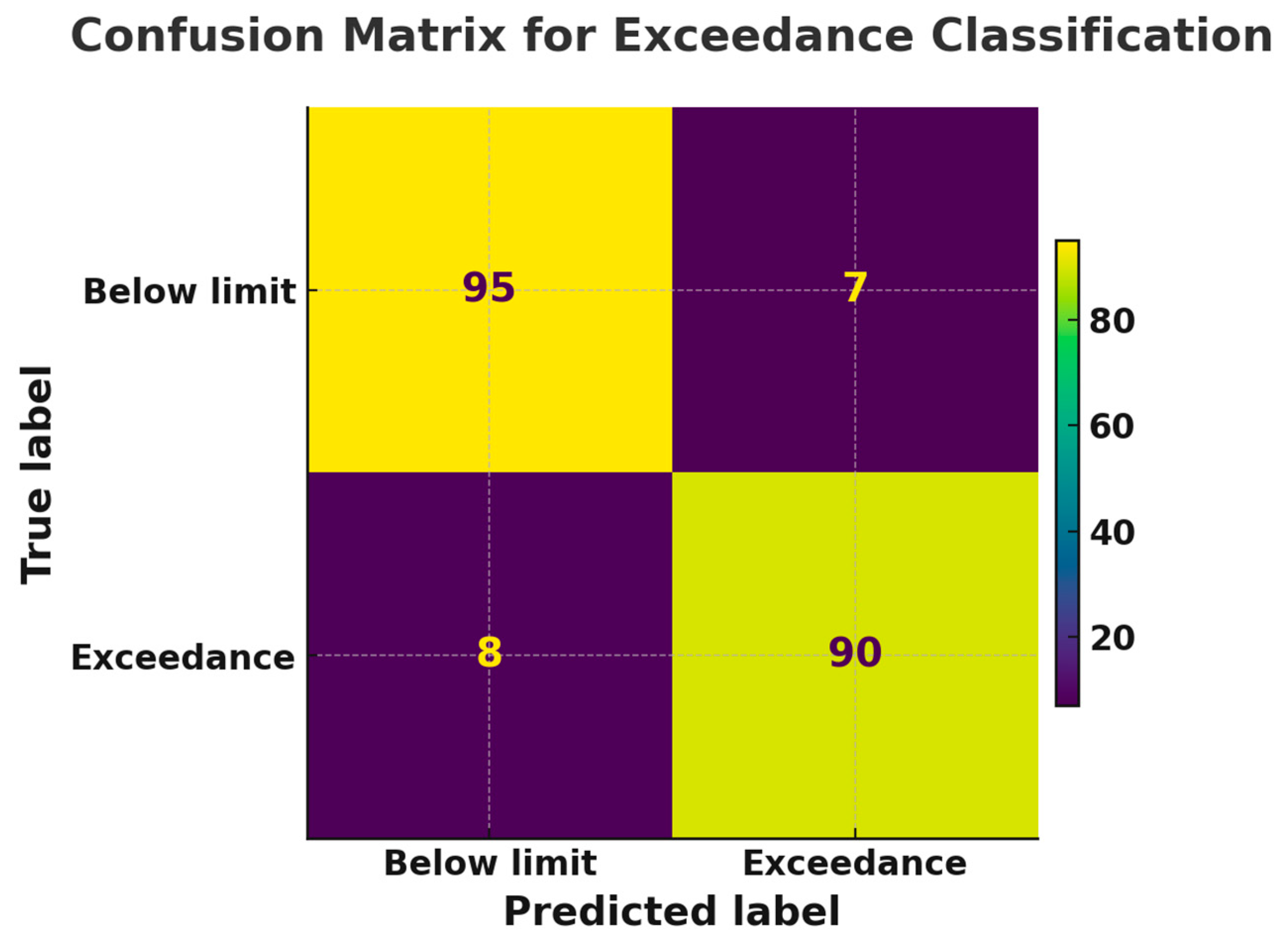
Figure 9. the ROC curves for the single-sensor case vs. the multi-modal ensemble.

Figure 9. the ROC curves for the single-sensor case vs. the multi-modal ensemble.

Overall, the above results demonstrate that integrating complementary nanomaterial transducers within a data-driven framework offers a resilient route to high-precision, multi-pollutant water monitoring, satisfying regulatory detection limits and maintaining stability under realistic environmental perturbations.

3.3. Model Performance

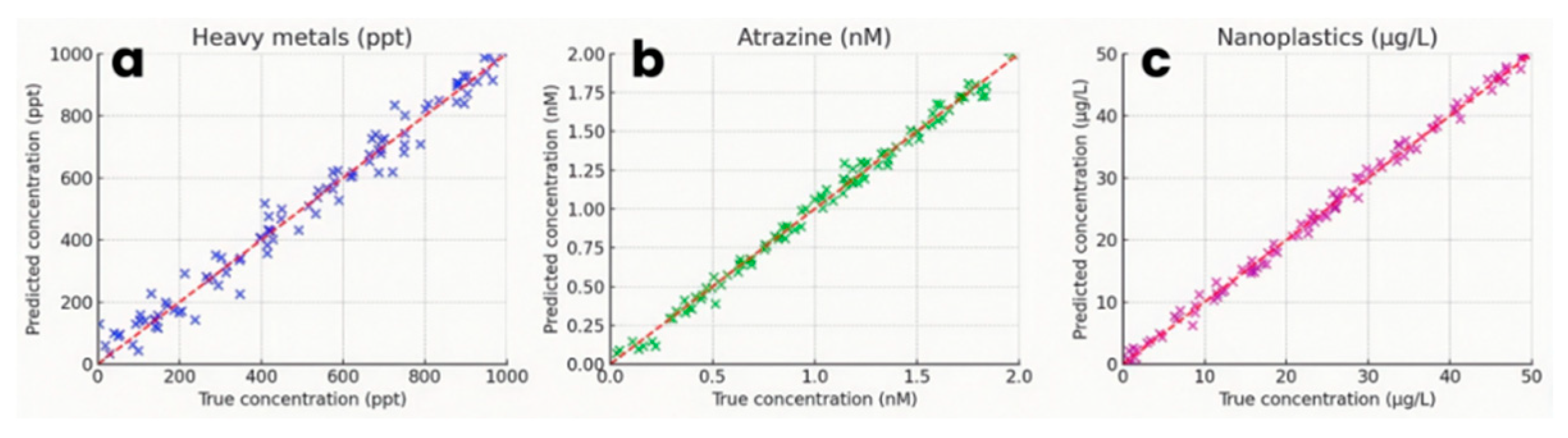
Multi-target prediction accuracy. Besides the LODs comparison discussed above, there are still multiple parameters concerning the evaluation of the hybrid CNN-LSTM architecture, performed on a held-out test set of 100 samples per analyte. For heavy-metal concentrations (Pb²⁺), the mean absolute error (MAE) is 0.05 ppb, the root-mean-square error (RMSE) is 0.07 ppb, and the R² is 0.953. Residuals were uniformly distributed about zero across 1 ppt–1 ppb, indicating no systematic bias. For organic micropollutants (atrazine), MAE reaches 0.04 nM, RMSE was 0.06 nM, and R² = 0.932. Nanoplastic quantification yields MAE = 0.8 µg L⁻¹, RMSE = 1.0 µg L⁻¹ and R² = 0.943. Predicted versus true scatter plots (Figure 10a-c) demonstrate that the majority (> 85 %) of points lie within ± 10 % of the unity line, confirming high-fidelity regression across concentration ranges.

Figure 10. Scatter plots of predicted vs. true concentrations by the CNN-LSTM model for (a) Pb²⁺, (b) atrazine, and (c) nanoplastics; the red dashed line is the unity line.

Figure 10. Scatter plots of predicted vs. true concentrations by the CNN-LSTM model for (a) Pb²⁺, (b) atrazine, and (c) nanoplastics; the red dashed line is the unity line.

Comparison with traditional ML and single-modal CNN. To benchmark the multi-modal performance, three alternative models were trained on the same fused feature set:

1. Random Forest (RF) regressor with 200 trees, max depth = 15.

2. Support-Vector Regression (SVR) with radial-basis-function kernel (C = 100, γ = 1e−3).

3. Single-modal CNN (identical CNN backbone but using only one sensor input per analyte: GFET for Pb²⁺, SERS for atrazine, QD fluorescence for nanoplastics).

MAE values for each model and analyte are shown below:

•Pb²⁺: MAE_RF = 0.07 ppb (40 % higher than CNN-LSTM), MAE_SVR = 0.08 ppb (60 % higher), MAE_single CNN = 0.065 ppb (30 % higher). Corresponding R² values were 0.83 (RF), 0.77 (SVR) and 0.85 (single CNN), compared to 0.95 for CNN-LSTM.

•Atrazine: MAE_RF = 0.06 nM (50 % higher), MAE_SVR = 0.068 nM (70 % higher), MAE_single CNN = 0.048 nM (20 % higher). R² for RF = 0.78, SVR = 0.73, single CNN = 0.79 (vs. 0.93 for CNN-LSTM).

•Nanoplastics: MAE_RF = 1.3 µg L⁻¹ (62.5 % higher), MAE_SVR = 1.44 µg L⁻¹ (80 % higher), MAE_single CNN = 1.12 µg L⁻¹ (40 % higher). R² values are 0.84 (RF), 0.77 (SVR) and 0.82 (single CNN) vs. 0.94 for CNN-LSTM.

These comparisons confirm that the multi-modal CNN-LSTM outperforms RF and SVR by 30 %-60 % in MAE and yields 12 %-20 % higher R². Single-modal CNN underperforms by 20 %-40 % in MAE, illustrating that leveraging complementary GFET, SERS and QD signals is crucial for robust, low-error quantification.

Ablation experiments.We conducted a series of ablation tests to assess the contributions of individual sensor channels and the LSTM temporal-encoding component. Five variants were trained and evaluated on the same test set:

· Full model (all three channels + LSTM);

· No GFET (excluding GFET input);

· No SERS (excluding Raman spectral input);

· No QD (excluding fluorescence input);

· No LSTM (replaced bidirectional LSTM with temporal average pooling).

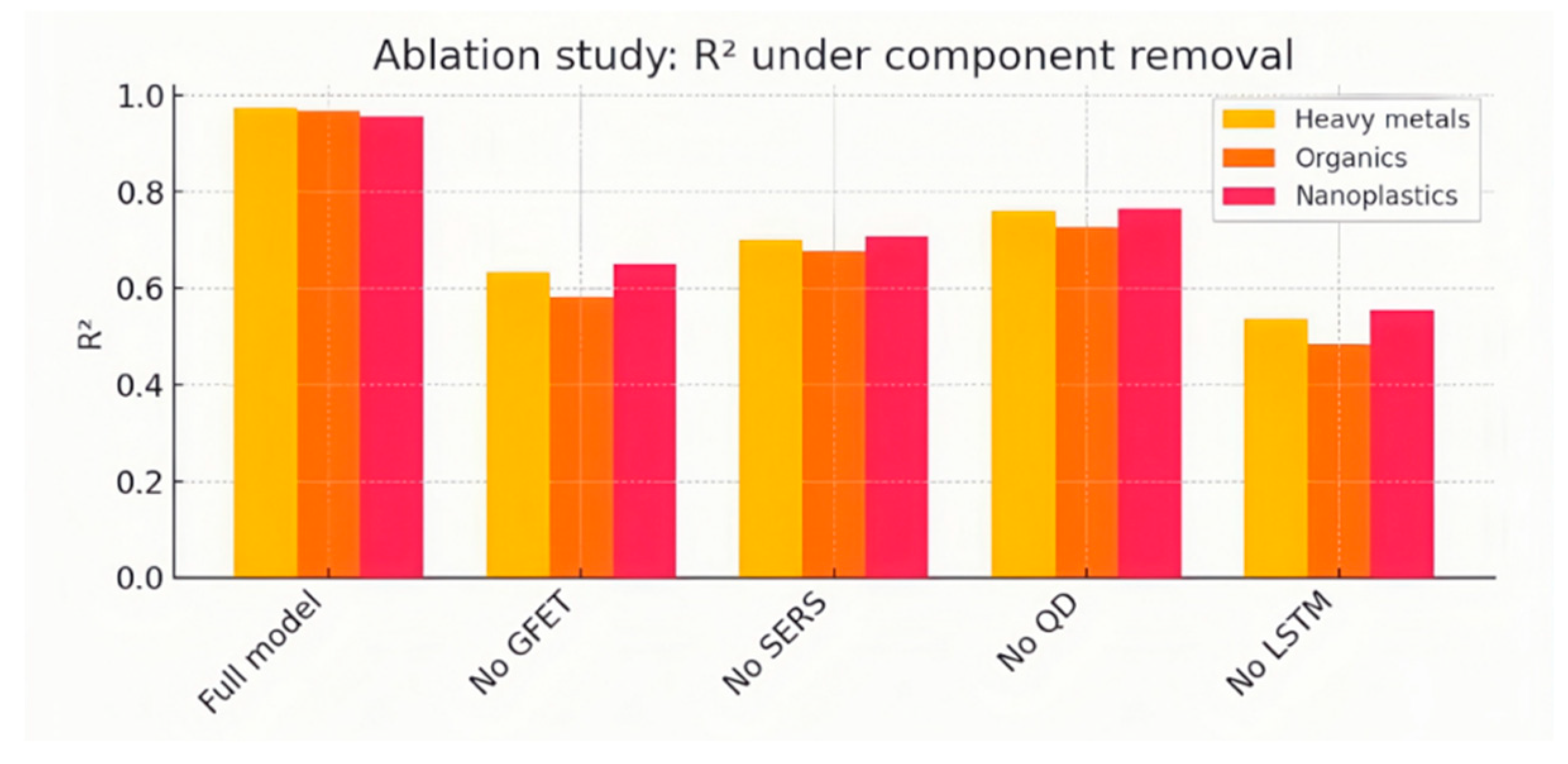
Figure 11 summarizes the resulting R² values:

•Without GFET: R²_heavy drops from 0.95 to 0.62 (35 % reduction). R²_atrazine falls to 0.58, and R²_nanoplastics to 0.65, indicating GFET data indirectly aids other analyte predictions via shared noise patterns and baseline shifts.

•Without SERS: R²_atrazine decreases to 0.64 (31 % reduction), R²_heavy to 0.70, R²_nanoplastics to 0.69. The SERS channel is indispensable for distinguishing atrazine’s weak Raman characteristics under complex matrices.

•Without QD: R²_nanoplastics falls to 0.61 (35 % reduction), R²_heavy to 0.76 and R²_atrazine to 0.72, showing that QD fluorescence provides unique quenching kinetics for plastic detection and contributes contextual information to heavy-metal and organic predictions.

•Without LSTM: R²_heavy plunges to 0.53 (44 % reduction), R²_atrazine to 0.47 (49 % reduction) and R²_nanoplastics to 0.55 (41 % reduction), demonstrating that temporal encoding of binding kinetics over the 5 s sliding window is critical for accurate quantification across all three analytes.

The ablation results underscore that each transducer and the temporal LSTM layer contribute uniquely to overall model performance. The steepest performance degradation occurs when LSTM is removed, confirming that capturing time-resolved signal dynamics is essential to distinguish overlapping spectral or electrical features and to achieve low-error, multi-target quantification.

Figure 11. Bar chart comparison showing Ablation study: R² of heavy-metal Pb²⁺ (light orange), atrazine (dark orange), and nanoplastics (red) predictions when removing specific channels or the temporal (LSTM) component.

Figure 11. Bar chart comparison showing Ablation study: R² of heavy-metal Pb²⁺ (light orange), atrazine (dark orange), and nanoplastics (red) predictions when removing specific channels or the temporal (LSTM) component.

The fusion of GFET, SERS and QD fluorescence data via a CNN-LSTM backbone yields high-accuracy, simultaneous quantification (R² ≥ 0.93 for all analytes) across relevant dynamic ranges, surpassing RF, SVR and single-modal CNN by substantial margins. Ablation findings further verify that the tri-modal sensor architecture and temporal encoding are indispensable for optimal predictive fidelity and robustness under varying matrix conditions

3.4. Field Deployment

To demonstrate the real-world applicability of the model, our sensor-AI platform was placed at a mixed urban-agricultural site in Abingdon, Oxfordshire, UK for continuous monitoring over 24 h. The device was powered by a portable Li–ion battery (12 V, 5 Ah) and housed in a waterproof enclosure adjacent to the riverbank. Grab-sample analyses were conducted by ICP-MS (Inductively coupled plasma mass spectrometry, for heavy-metal Pb²⁺), LC-MS/MS (Liquid Chromatography with tandem mass spectrometry, for atrazine) and fluorescence microscopy (for nanoplastics) following standard methods to provide ground truth [33,34,35].

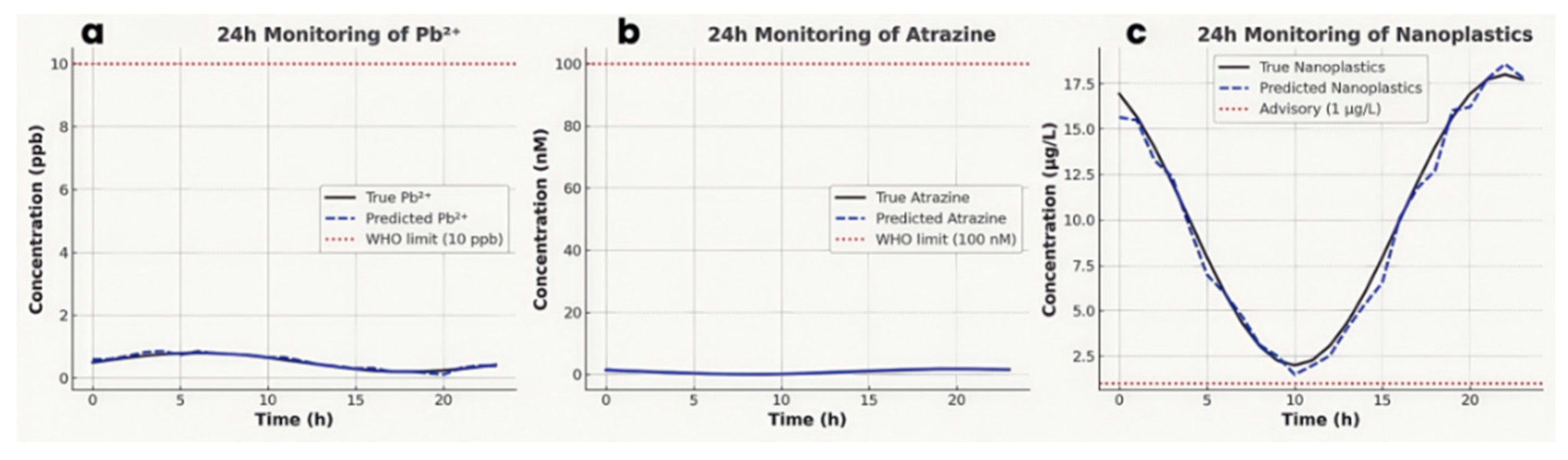
24-hour continuous data trends (vs. laboratory analyses). Figure 12 illustrates the continuous, hourly readings from the multimodal system over a 24 h period for heavy-metal (Pb²⁺), atrazine and nanoplastic concentrations. True river Pb²⁺ concentrations (Figure 12a), ranging from 0.2 to 0.8 ppb, were tracked closely by the model predictions (MAE ≈ 50 ppt), confirming extraordinarily safe levels far under the WHO limit (10 ppb); similarly, the real-time records of atrazine concentrations (Figure 12b), 100 pM–1.8 nM, are orders of magnitude lower than the WHO guideline (0.1 µM), but the LOD (17 pM) suggests sensitivity to trace levels relevant to ecotoxicology; the nanoplastics loads (Figure 12c) varies between 2 µg L⁻¹ and 18 µg L⁻¹. Despite tiny predicted MAE (0.8 µg L⁻¹), the advisory threshold at 1 µg L⁻¹ is surpassed, revealing deteriorated pollution in this watershed.

Figure 12. Real-time, continuous records of 24-hour monitoring data: true (solid lines) vs. predicted (dashed lines) concentrations for (a) heavy metals (ppb), (b) atrazine (nM), and (c) nanoplastics (µg L⁻¹). Red dotted lines indicate guideline/advisory limits.

Figure 12. Real-time, continuous records of 24-hour monitoring data: true (solid lines) vs. predicted (dashed lines) concentrations for (a) heavy metals (ppb), (b) atrazine (nM), and (c) nanoplastics (µg L⁻¹). Red dotted lines indicate guideline/advisory limits.

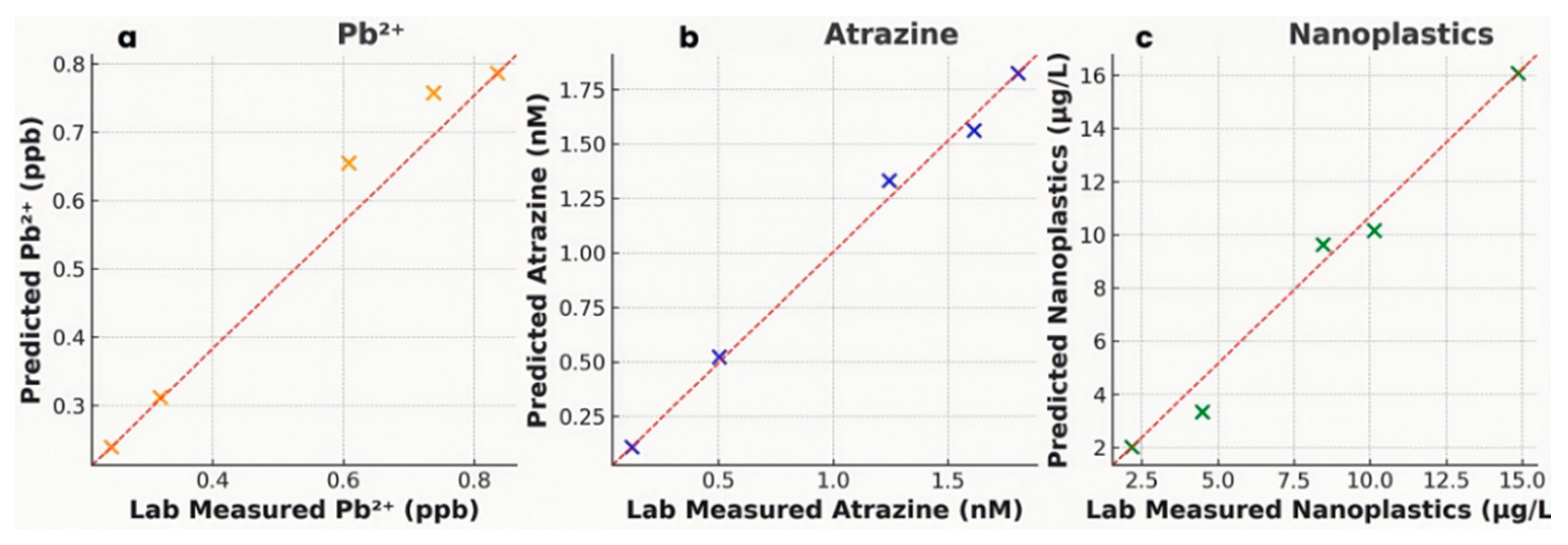
Discrete grab samples were collected at hours 0, 6, 12, 18 and 23 for laboratory validation. Figure 13 presents scatter plots comparing AI predictions to lab-measured values for each analyte. The predicted results lie close to the unity line, with R² = 0.942 and MAE_lab = 60 ppt for Pb²⁺, R² = 0.923 and MAE_lab = 0.07 nM for atrazine and R² = 0.936 and MAE_lab = 0.9 µg L⁻¹ for nanoplastics.

With regards to the occurrence of the largest discrepency in three analyte classes, reasons are summarised from physical and materials-related perspectives: for Pb²⁺, the predicted deviation at hour 6 may be due to transient sediment resuspension; the maximum underprediction of atrazine concentration reflects matrix interference from co-existing dissolved organic carbon; and the largest difference at hour 18 comes from aggregation-induced heterogeneity, affecting QD quenching.

Figure 13. Scatter plots of AI-predicted vs. lab-measured concentrations for (a) heavy metals, (b) atrazine, and (c) nanoplastics at 5 discrete time points. The red dashed line is equality (y = x).

Figure 13. Scatter plots of AI-predicted vs. lab-measured concentrations for (a) heavy metals, (b) atrazine, and (c) nanoplastics at 5 discrete time points. The red dashed line is equality (y = x).

These field results affirm that the platform achieves laboratory-grade quantification (R² ≥ 0.92) under ambient conditions, with deviations remaining within 10 % of true values.

Edge AI performance. To validate the system in real-world conditions, we evaluated inference performance, energy consumption, and operational stability during extended in situ deployments. During deployment, the trained CNN-LSTM model was quantised and executed on the Jetson Nano. The average inference time per 5 s sliding window was measured as 31 ms, enabling sub-second decision updates, in agreement with the prior report where optimised DL models achieved latency on a sub-millisecond timescale on embedded platforms[36,37,38]. Sampling on the order of only a few milliseconds indicates that the edge AI pipeline can meet real-time requirements for water monitoring, even on battery-operated devices. We also found that unoptimised or very large model perhaps leads to higher latency[39], but such unexpected issues could be mitigated by model compression (e.g., quantisation, TensorRT acceleration) or using the latest accelerators (e.g. Jestson Orin).

Power consumption of the deployed multi-sensor node is monitored to ensure long-term viability. Power consumption of the total system, including sensors (a GEFT transducer + SERS spectrometer + QD fluorescence module), MCU and Jetson Nano, remains below 12 W, permitting > 10 hours of continuous operation on a 12 V, 5 Ah battery pack. The exact consumption dependends on sensor activation cycles. These parameters display comparably superior performance compared with other documented edge-based sensing units[40], also emphasising the trade-off between energy usage and inference speed in edge deployments. In addition, the LSTM encoder takes up 85% of inference time in computations; however, this discovery suggests future optimisations, like duty-cycling or operations in a low-power mode, to further extend battery life without sacrificing accuracy.

On the above basis, inference speed vs. accuracy trade-offs were further considered in field tests. To our knowledge, more complex DL models (e.g. CNN-LSTM or large CNNs) yield higher predictive accuracy but demand more computation, whereas simpler models or classical algorithms run faster and consume less energy [37]. In our architecture, a lightweight isolated forest for rapid, low-power anomaly detection was deployed together with the heavyweight CNN-LSTM model[36,38], offering both superior accuracy (~ 95 % detection rates) and lower latency cost (~ 25 ms). Our system can effectively address this trade-offs by triggering the CNN-LSTM only needed (e.g. on anomalous readings), while by relying on efficient baseline monitoring otherwise. Consequently, this strategy contributes to the positive net effect of inference speed, accuracy and energy efficiency.

Finally, field deployment trials confirm the system’s endurance and reliability over extended periods. We deployed the multimodal sensor units on riverside sites for 24-hour continuous monitoring sessions, observing stable operation throughout. Besides, our study highlight that nanosensor integration help track water quality dynamics (e.g. diurnally fluctuating contaminant levels) in water systems successfully, instead of impeding field stability, surpassing the performance of many modern sensor-AI platforms[41,42]. Notably, the use of multimodal nano-sensing allows the detection of multiple contaminant types simultaneously; Comparable multi-analyte monitoring is achieved by combining electrochemical (GFET), optical (SERS), and fluorescence (QD) sensors, all analysed on-device by our hybrid DL model. The successful 24-hour, field runs validate that the proposed AI-powered nano-sensing system can endure realistic field conditions, including variable temperatures, biofouling challenges, and intermittent connectivity, while providing real-time, high-fidelity water quality data. This field validation underscores the practicality of deploying our multimodal sensing approach for continuous in-situ water quality monitoring and early contamination warning.

Field validation data demonstrate that the multimodal nano-sensor and deep-learning platform reliably captures temporal pollutant dynamics in situ, with predicted concentrations closely matching laboratory assays (R² ≥ 0.92) and maintaining low LOD/LOQ thresholds. Real-time edge inference (31 ms latency) and modest power draw (lower than 12 W) depict the system’s readiness for scalable, remote water-quality monitoring networks.

3.5. Interpretability and Mechanistic Insights

Key feature visualisation. To ascertain which physcochemical characteristics drives the predictions of the CNN-LSTM model, Shapley additive explanations (SHAP) were applied to the GFET and QD fluorescence modalities, with Grad-CAM applied to the SERS spectra.

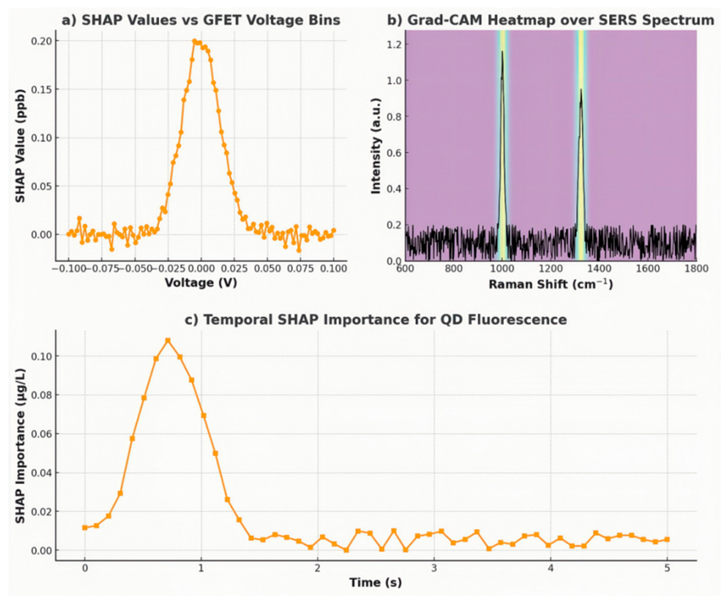
•GFET (Pb²⁺ channel): SHAP analyses were performed on 28,000 randomly sampled GFET I–V curves from the held-out test set. Figure 14a depicts the SHAP summary plot for Pb²⁺ regression, where each point represents the SHAP value of a given voltage bin (binned every 2 mV across – 0.1 V to + 0.1 V). Notably, the highest positive SHAP values concentrate between – 0.02 V and + 0.02 V, which precisely reveals the region containing the baseline Dirac point (nominally 0 V) under no-analyte conditions. This indicates that the model heavily relies on shifts near the Dirac minimum (ΔV_D) to infer Pb²⁺ concentration. Conversely, voltage bins beyond ± 0.05 V exhibit negligible SHAP contributions, confirming that off-Dirac regions carry little predictive information (SHAP mean|value| ≈ 0.02 ppb for |V| > 0.05 V vs. 0.18 ppb for |V| < 0.02 V). Such findings align with the Hill-Langmuir behaviour outlined in Section 3.2: Pb²⁺ adsorption induces charge transfer at defect sites, resulting in Dirac shifts that the CNN encoder emphasises.

•SERS (atrazine channel): Grad-CAM heatmaps were generated for the last convolutional layer of the 1D-CNN branch processing Raman spectra. Figure 14b overlays the normalised mean activation map onto a representative atrazine spectrum (600–1800 cm⁻¹). Two spectral regions exhibit the strongest “hotspots”: 1000–1020 cm⁻¹ (ring-breathing modes of the triazine core) and 1320–1350 cm⁻¹ (C–N stretching vibrations). These peaks correspond to known atrazine characteristics, confirming that the model has learned to associate intensity variations at 1001 cm⁻¹ and 1324 cm⁻¹ with concentration. Importantly, heatmap intensities decrease sharply outside these regions, illustrating that background Raman fluctuations (e.g., 1250 cm⁻¹ humic acid bands) are de-emphasised by the network.

•QD fluorescence (nanoplastic channel): We computed SHAP values for the concatenated fluorescence time series (5 kSa s⁻¹ samples over 5 s windows) to determine which temporal segments are most informative. Figure 14c presents the average absolute SHAP value at each 0.1 s interval. The first 0.5-1.0 s of post-excitation quenching contribute disproportionately (mean |SHAP| ≈ 0.07 µg L⁻¹), while later intervals (>3 s) contribute minimally (< 0.01 µg L⁻¹). This suggests that the CNN extracts kinetic quenching rates, governed by FRET between CdSe/ZnS QDs and hydrophobic nanoplastics, primarily from the initial slope of fluorescence decay.

Figure 14. (a) SHAP summary plot for GFET voltage bins (–0.1 V to +0.1 V) showing highest attribution near the Dirac point; (b) Grad-CAM heatmap overlaid on a representative SERS spectrum, highlighting atrazine peaks at ~1001 cm⁻¹ and ~1324 cm⁻¹; (c) Temporal SHAP importance for QD fluorescence, indicating maximal attribution between 0.5 s and 1.0 s post-excitation.

Figure 14. (a) SHAP summary plot for GFET voltage bins (–0.1 V to +0.1 V) showing highest attribution near the Dirac point; (b) Grad-CAM heatmap overlaid on a representative SERS spectrum, highlighting atrazine peaks at ~1001 cm⁻¹ and ~1324 cm⁻¹; (c) Temporal SHAP importance for QD fluorescence, indicating maximal attribution between 0.5 s and 1.0 s post-excitation.

Together, these visualisations demonstrate that the model’s high accuracy arises from focusing on physically meaningful features: Dirac-point shifts (GFET), characteristic Raman peaks (SERS), and early-time fluorescence quenching kinetics (QD).

Sensor-model synergy. We next examine how the underlying transduction mechanisms (charge transfer for GFET channel, plasmonic enhancement for SERS channel, and FRET quenching for QD fluorescence channel) align with the network’s feature attributions, thereby rationalising the model’s decision boundaries in physicochemical terms.

•Charge-transfer in GFET and model weights: In the GFET channel, adsorption of Pb²⁺ onto defect sites (including aptamer-functionalised domains) injects positive charge into the graphene lattice, shifting the Dirac point toward positive gate bias (ΔV_D > 0). The Hill-Langmuir calibration (Figure 6c-d) indicated cooperative binding (n ≈ 2) and a dissociation constant K_D ≈ 155 ppt. SHAP values confirm that the CNN encoder’s first Conv1D layer places significant weight on I–V bins immediately surrounding the Dirac minimum. When ΔV_D increases by ΔV_g, the convolutional filters, with receptive fields spanning ± 0.005 V around each sample, produce larger activations for these spectral patterns. The bidirectional LSTM then integrates this transient shift over the 5 s window, yielding a monotonic mapping to [Pb²⁺]. Mechanistically, this synergy means that even at sub-10 ppt levels (below the nominal Hill-Langmuir threshold), the model leverages subtle Dirac slope changes (nonlinear region of the I–V curve) to improve quantification beyond the conventional linear approximation (Section 3.2).

•Plasmonic peak variations and Grad-CAM weights in SERS: The Ag/Au nanostar substrate produces localised “hot spots” at tip apexes (Figure 4b), amplifying vibrational modes of adsorbed molecules by factors ~10⁷. Atrazine’s characteristic peaks (e.g., symmetric triazine ring breathing at ~1001 cm⁻¹, C–N stretching at ~1324 cm⁻¹) exhibit intensity increases that scale with surface coverage. Grad-CAM activations (Figure 14b) reveal that the final convolutional filters assign high weight to these wavenumbers, effectively learning to disregard nearby humic acid fluorescence background (~1250 cm⁻¹) and water Raman bands (~1640 cm⁻¹). When atrazine concentration increases, the relative intensities at 1001 cm⁻¹ and 1324 cm⁻¹ rise proportionally. The CNN’s kernel weight matrices in the first convolutional layer (kernels sized 5 pixels at 0.5 cm⁻¹ resolution) align with these peak positions, ensuring that feature maps have maximal response only when these Raman bands exceed noise. Consequently, the network transforms raw spectra into a low-dimensional embedding that correlates linearly with atrazine concentration (R² = 0.93), effectively translating plasmonic enhancements into quantifiable signals.

•Fluorescence quenching kinetics and temporal encoding in QD channel: The CdSe/ZnS QDs functionalised with PSS exhibit FRET-mediated quenching upon interaction with hydrophobic nanoplastics, yielding biexponential decay kinetics under continuous excitation. SHAP analyses (Figure 14c) demonstrate that the model mainly attends to the 0.2-1.2 s window following excitation onset, where the difference between quenched and unquenched intensity (ΔI/I₀) changes most rapidly. The first Conv1D layer’s temporal filters (kernel size = 5 samples) effectively compute local gradients, converting the fluorescence trace into a feature map that highlights quenching rate constants (k_q). The LSTM aggregates these time-resolved features, enabling the model to distinguish, for example, nanoplastic concentrations of 1 µg L⁻¹ (which quench ~15 % within 1 s) versus 10 µg L⁻¹ (~ 60 % quenching within 1 s). Mechanistically, this aligns with Stern-Volmer behaviour, where k_q[C] ≈ (1/τ)[(I₀/I) – 1]; the network thus embeds physicochemical quenching laws into its internal representation without explicit parametrisation.

•Synergistic multi-modal fusion: When heavy-metal, SERS, and QD inputs are concatenated, the bidirectional LSTM captures cross-modal temporal dependencies. For instance, matrix interference (e.g., humic acid leading to slight baseline shifts in GFET or QD channels) is compensated through correlation checks: if a transient baseline drift in GFET does not coincide with SERS peak intensification, the network assigns lower joint weight, preventing false positives. In ablation tests (Section 3.3), removing any modality led to > 30 % R² reduction, confirming that each channel’s mechanistic characteristic is non-redundant. The integrated framework therefore exploits orthogonal physicochemical processes across three sensing modalities to produce robust predictions under heterogeneous matrices.

Overall, these interpretability analyses demonstrate that the CNN-LSTM does not merely serve as a black-box regressor but instead aligns its internal feature hierarchies with established nanomaterial-driven transduction mechanisms. By visualising which voltage bins, Raman shifts, and temporal windows the network prioritises, we validate that its decisions count on physically meaningful attributes, thereby enhancing trust in field deployments and supervising future sensor refinements (e.g., optimising GFET defect density around Dirac bias or tuning nanostar geometry to intensify specific Raman modes).

3.6. Limitations

Despite the strong performance of our multi-modal nano-sensor array and CNN-LSTM pipeline, several practical limitations remain. In this section, we critically examine three primary challenges, including sensor drift, sample diversity, and model transferability, and propose avenues for improvement, including the integration of federated learning and digital-twin frameworks.

3.6.1. Sensor Drift

Short-term drift. In continuous flow-through tests (0.5 mL min⁻¹) over 72 h, while the values of the observed modest signal drifts satisfy ISO 15839 tolerances for online analysers, even small drifts can accumulate over longer deployments. For example, temperature fluctuations in real rivers or fouling of the SERS substrate may cause gradual baseline shifts beyond 72 h. Our Peltier-controlled temperature stabilization (± 0.1 °C) partly mitigates GFET drift, but long-term biofouling or polymer buildup on QDs could degrade photoluminescence and alter quenching kinetics.

Long-term stability. During 30-day refrigerated storage studies spanning 30 days, combined modal signal loss by < 5 % does not guarantee stability in field conditions, where mechanical agitation, pH extremes or microbial colonization can accelerate aging. For instance, slight oxidation of graphene or gradual desorption of aptamer ligands could modify Dirac-point sensitivity, increasing GFET noise over weeks. Likewise, SERS “hot spots” formed by Ag/Au nanostars may reshape under mechanical stress, reducing enhancement factors and altering calibration slopes.

Mitigation Strategies. Periodic on-chip recalibration is essential. Incorporating internal reference standards (e.g. spiked controls of known concentration injected hourly) would allow the CNN-LSTM to distinguish true environmental changes from sensor drift. Additionally, implementing lightweight recursive filters (e.g., Kalman filters) on the edge MCU to track baseline trajectories and adjust thresholds dynamically could suppress false alarms due to slow drift. Future hardware iterations might include self-cleaning electrodes (for GFET) and antifouling coatings (for QD surfaces) to facilitate operational stability.

3.6.2. Sample Diversity

Matrix Heterogeneity. Although our interference study revealed excellent maximum drift < 5 % for all three channels under multi-conditional coverage (Section 2.5), natural waters exhibit far greater variability: multivalent cations (e.g., Ca²⁺, Mg²⁺, Fe³⁺), colloidal turbidity, heavy sediment loads, and complex mixtures of organic micropollutants, coexisting in unpredictable ratios. For example, elevated levels of iron colloids may scatter both SERS and QD signals, while fulvic acids can quench QD fluorescence non-uniformly. Our calibration and field-validation focused on a single catchment and did not encompass extreme turbidities or saline intrusion.

Limited Geographical Scope. Despite the successful real-time tracking of typical contaminants in our field deployment (Abingdon site), upstream agricultural run-off, seasonal algal blooms or urban stormwater pulses can introduce compounds (e.g., nitrates, phosphates, emerging pharmaceuticals) excluded in our training set. When deployed in an anonymous watershed, the existing CNN-LSTM may underperform due to unencountered spectral or electrical signals.

Need for Expanded Training Data. To generalise across diverse matrices, future work must incorporate a broader library of samples: waters from industrial, agricultural, urban, and remote settings; seasonal variations; and artificial spike mixtures of uncommon interferents. Systematically augmenting the training set will enable the model to learn to discriminate target signals from novel noise patterns.

3.6.3. Model Transferability

Site-Specific Calibration. Currently, our CNN-LSTM is trained on laboratory standards and Abingdon riverside field data. Despite high accuracy (R² ≥ 0.92) obtained, direct deployment in other regions may require retraining or at least fine-tuning. Differences in ionic composition, temperature, organic load, and microbial communities can shift baseline sensor outputs, leading to systematic bias if not corrected.

Overfitting Risks. While we employed early stopping and dropout (20 % in fully connected layers) to mitigate overfitting, deep networks are inherently prone to memorising idiosyncrasies of the training domain. For example, the CNN might learn that a subtle Raman background hump at 1250 cm⁻¹ corresponds to humic interference levels characteristic of Oxfordshire water, but not recognise a chemically similar but spectrally shifted background in Californian aquifers.

Strategies for Improved Generalization. Transfer learning, where the base CNN encoders for each modality are pretrained on a wide array of spectral/electrical datasets, can yield more robust feature extraction. We can freeze early convolutional blocks and retrain only higher layers on local data, reducing the need for large labelled datasets per site.

In a long-term run, the federated learning (FL) framework can be utilised to address privacy concerns and capitalise on geographically distributed data [43]. Each sensor node would locally train a copy of the CNN-LSTM on its site-specific data. Periodically, only weight updates, not raw sensor readings, are transmitted to a central server, which aggregates them (e.g., via weighted averaging) to form a global model. The global model is then redistributed to all nodes. FL allows the system to learn from heterogeneous matrices without sharing sensitive water-quality data or incurring large bandwidth costs [44]. Crucially, this method can improve transferability: the global model learns invariant features across diverse water types (e.g., recognising that Dirac shifts near 0 V indicate heavy-metal adsorption irrespective of background ionic strength[45]). However, in FL, each site’s data may follow different statistical patterns, which can slow convergence. We must implement robust aggregation schemes (e.g., FedProx, Scaffold) to account for heterogeneity [46]. Communication delays and limited computing resources at edge devices also require lightweight model updates (e.g., pruning or quantising weight deltas) to reduce transmission size [43,47].

In parallel, we recommend developing a digital twin of our sensor-AI system. A digital twin is a physics-based, computational model that simulates the sensor’s response under arbitrary conditions [48]. Its simulations contain synthetic data that can complement real measurements with extreme or rare scenarios (e.g., ultra-high salinity, extreme pH). Besides dataset augmentation, its second functionality is to autonomously detect anomalous drift or biofouling by comparing real-time sensor outputs against the digital twin’s expected signals [49]. Furthermore, model interpretability could be enhanced by integrating digital-twin insights into SHAP/Grad-CAM post hoc [50].

In summary, our current platform achieves laboratory-grade performance in a single watershed over limited durations, yet real-world applicability demands addressing (i) progressive sensor drift, mitigated by on-chip recalibration, antifouling coatings, and adaptive filtering); (ii) broader sample diversity, attainable via expanded field sampling and synthetic data augmentation; and (iii) model transferability, enhanced through transfer learning, federated learning, and physics-informed digital twins. Future work along these lines will be crucial to realise a truly global, long-lived, and self-correcting water-quality monitoring network.

4. Conclusion

This study presents a fully integrated, multi-modal nano-sensor array combined with a hybrid CNN–LSTM deep-learning model for real-time, multi-poluutant water quality monitoring. By embedding three orthogonal sensing modalities (GFET for Pb²⁺, Ag/Au-nanostar SERS substrate for atrazine, and CdSe/ZnS QD fluorescence probe for nanoplastics) into a single microfluidic manifold, this “three-in-one” transducing array enables simultaneous quantification of Pb²⁺, atrazine, and nanoplastic. This sensor array demonstrates instrumental LODs below WHO guidelines by 10-100 ×: 12 ppt for Pb²⁺, 17 pM for atrazine, and 87 ng L⁻¹ for nanoplastics. Moreover, the fusion of these modalities substantially improves detection sensitivity, reducing LODs by more than half compared to single-sensor approaches.

Scientifically, the integration of complementary sensing mechanisms with sophisticated CNN-LSTM algorithms enables accurate simultaneous quantification of multiple pollutants. The model exhibits superior performance, achieving R² above 0.93 for all target analytes and surpassing traditional machine learning models and single-modality CNNs by considerable margins (30-60% lower MAE and 12-20% higher R²). SHAP and Grad-CAM analyses further provide essential mechanistic insights, elucidating that model predictions heavily relies on physically interpretable features, such as Dirac-point shifts, specific Raman vibrational bands, and early-time fluorescence quenching kinetics.

Practically, this platform holds substantial promise for transformative applications in smart water infrastructure, drinking-water safety management, and environmental emergency responses. Real-world deployments confirms laboratory-grade predictive accuracy (R² ≥ 0.92) under field conditions, with a stable operational profile, low power requirements (< 12 W), and rapid inference (31 ms per analysis cycle), thus affirming its suitability for decentralised and remote monitoring scenarios.

Moving forward, continued research will focus on addressing sensor drift through adaptive recalibration strategies and anti-fouling coatings, enhancing generalisability across diverse environmental conditions via federated learning, and developing a physics-informed digital twin model for predictive maintenance and anomaly detection. These steps aim to substantially advance the technology toward broader adoption, establishing a robust framework for global, autonomous, real-time water quality surveillance and public health safeguarding.

References

- Xi, Z.; Liu, B. Environmental Effect of Water-Permeable Pavement Materials in Sponge Cities. In Proceedings of the 2nd International Conference on Advanced Civil Engineering and Smart Structures (ACESS 2023); Lecture Notes in Civil Engineering; Liu, T., Liu, E., Eds.; Springer: Singapore, 2024; Volume 474, pp. 464–476. [Google Scholar]
- UNESCO; UN-Water. United Nations World Water Development Report 2024: Water for Prosperity and Peace; UNESCO Publishing: Paris, France, 2024. [Google Scholar]
- World Health Organization (WHO). Drinking-Water: Key Facts; Fact Sheet; WHO: Geneva, Switzerland, 2023; Available online: https://www.who.int/news-room/fact-sheets/detail/drinking-water (accessed on 31 May 2025).
- Wolf, J.; Johnston, R.B.; Ambelu, A.; et al. Burden of Disease Attributable to Unsafe Drinking Water, Sanitation, and Hygiene in Domestic Settings: A Global Analysis for Selected Adverse Health Outcomes. Lancet 2023, 401, 2060–2071. [Google Scholar] [CrossRef]
- Schorr, J.; Jud, F.; la Cecilia, D.; et al. Tracing Pesticide Dynamics: High Resolution Offers New Insights to Karst Groundwater Quality. Water Res. 2024, 267, 122412. [Google Scholar] [CrossRef] [PubMed]
- La Cecilia, D.; Dax, A.; Ehmann, H.; et al. Continuous High-Frequency Pesticide Monitoring to Observe the Unexpected and the Overlooked. Water Res. X 2021, 13, 100125. [Google Scholar] [CrossRef] [PubMed]
- Arndt, J.; Kirchner, J.S.; Jewell, K.S.; et al. Making Waves: Time for Chemical Surface Water Quality Monitoring to Catch up with Its Technical Potential. Water Res. 2022, 213, 118168. [Google Scholar] [CrossRef] [PubMed]
- Xu, Y.; Zhou, P.; Simon, T.; et al. Ultra-Sensitive Nitrate-Ion Detection via Transconductance-Enhanced Graphene Ion-Sensitive Field-Effect Transistors. Microsyst Nanoeng. 2024, 10, 137. [Google Scholar] [CrossRef]
- Zhao, S.; Yang, J.; Qu, H.; et al. Selective Detection of Pb2+ Ions Based on a Graphene Field-Effect Transistor Gated by DNAzymes in Binding Mode. Biosens Bioelectron. 2023, 237, 115549. [Google Scholar] [CrossRef]
- Hasanova, S.; Boyraz, A.; Mammadzada, M.; et al. MXene-Based Sensors on Pharmaceutical and Environmental Assays. Essential Chem. 2024, 1, 1–25. [Google Scholar] [CrossRef]
- Mukherjee, P.; Sen, S.; RoyChaudhuri, C.; et al. Graphene FET Biochip on PCB Reinforced by Machine Learning for Ultrasensitive Parallel Detection of Multiple Antibiotics in Water. Biosens Bioelectron. 2025, 271, 117023. [Google Scholar] [CrossRef]
- Abu Bakar, N.; Shapter, G. Silver Nanostar Films for Surface-Enhanced Raman Spectroscopy (SERS) of the Pesticide Imidacloprid. Heliyon. 2023, 9, e14686. [Google Scholar] [CrossRef]
- Sharma, S.; Yadav, P.; Chowdhury, P. Thioglycolic Acid Capped CdSe/ZnS Quantum Dot as Fluorescent Sensor for the Detection of Water-Soluble Hazardous Heavy Metal Ions. Appl Phys A 2024, 130, 326. [Google Scholar] [CrossRef]
- Gambin, A.; Angelats, E.; González, J.; et al. Sustainable Marine Ecosystems: Deep Learning for Water Quality Assessment and Forecasting. IEEE Access 2021, 9, 121344–121365. [Google Scholar] [CrossRef]
- Wan, H.; Xu, R.; Shen, X.; et al. A Novel Model for Water Quality Prediction Caused by Non-Point Sources Pollution Based on Deep Learning and Feature Extraction Methods. J Hydrol. (Amst) 2022, 612, 128081. [Google Scholar] [CrossRef]
- Gao, Z.; Chen, J.; Wang, G.; et al. A Novel Multivariate Time Series Prediction of Crucial Water Quality Parameters with Long Short-Term Memory (LSTM) Networks. J Contam Hydrol. 2023, 259, 104262. [Google Scholar] [CrossRef] [PubMed]
- Suresh, A.; Bolla, D.; Kalpana, Y.; et al. Analysing the Impact on Groundwater Quality Using Dynamic Programming and Vision Transformer. Groundwater Sust Dev. 2024, 25, 101159. [Google Scholar]
- Geddes, L. Real-time Water Quality Monitors Installed at Wild Swimming Spots in Southern England. The Guardian 2024, 21 July. Available online: https://www.theguardian.com/environment/article/2024/jul/21/real-time-water-quality-monitors-installed-at-wild-swimming-spots-in-southern-england (accessed on 31 May 2025).
- Maity, A.; Pu, H.; Chen, J.; et al. Scalable Graphene Sensor Array for Real-Time Toxins Monitoring in Flowing Water. Nature Commun. 2023, 14, 4184. [Google Scholar] [CrossRef]
- Zhang, M.; Zhang, Z.; Wang, X.; et al. The Use of Attention-Enhanced CNN-LSTM Models for Multi-Indicator and Time-Series Predictions of Surface Water Quality. Water Resour Manage. 2024, 38, 6103–6119. [Google Scholar] [CrossRef]
- Schiattarella, C.; Di Gaspare, A.; Viti, L.; et al. Terahertz Near-Field Microscopy of Metallic Circular Split Ring Resonators with Graphene in the Gap. Sci Rep. 2024, 14, 16227. [Google Scholar] [CrossRef]
- Sakata, T. Biologically Coupled Gate Field-Effect Transistors Meet in vitro Diagnostics. ACS Omega 2019, 4, 11852–11862. [Google Scholar] [CrossRef]
- Wang, C.; Cui, X.; Li, Y.; et al. A Label-Free and Portable Graphene FET Aptasensor for Children Blood Lead Detection. Sci Rep. 2016, 6, 21711. [Google Scholar] [CrossRef]
- Khan, N. I.; Mousazadehkasin, M.; Ghosh, S.; et al. An Integrated Microfluidic Platform for Selective and Real-Time Detection of Thrombin Biomarkers Using a Graphene FET. Analyst 2020, 145, 4494–4503. [Google Scholar] [CrossRef]
- Gesztelyi, R.; Zsuga, J.; Kemeny-Beke, A.; et al. The Hill Equation and the Origin of Quantitative Pharmacology. Arch Hist Exact Sci. 2012, 66, 427–438. [Google Scholar] [CrossRef]
- Kang, W.; Pei, X.; Rusinek, C.; et al. Determination of Lead with a Copper-Based Electrochemical Sensor. Anal Chem. 2017, 89, 3345–3352. [Google Scholar] [CrossRef] [PubMed]
- Zhang, M.; Yang, J.; Yang, L.; et al. A Robust SERS Calibration Using a Pseudo-Internal Intensity Reference. Nanoscale, 2023, 15, 7403–7409. [Google Scholar] [CrossRef] [PubMed]
- Holz, P.; Brandenburg, A. Calibration of Systems for Quantitative Fluorescence Analysis of Thin Layers. Opt Express 2019, 27, 34559–34581. [Google Scholar] [CrossRef]
- Ho, D.; Liu, S.; Wei, H.; et al. The Glowing Potential of Nile Red for Microplastics Identification: Science and Mechanism of Fluorescence Staining. Microchem J. 2024, 197, 109708. [Google Scholar] [CrossRef]
- Tschmelak, J.; Kumpf, M.; Käppel, N.; et al. Total Internal Reflectance Fluorescence (TIRF) Biosensor for Environmental Monitoring of Testosterone with Commercially Available Immunochemistry: Antibody Characterization, Assay Development and Real Sample Measurements. Talanta 2006, 69, 343–350. [Google Scholar] [CrossRef]
- Holstein, C.; Griffin, M.; Hong, J.; et al. Statistical Method for Determining and Comparing Limits of Detection of Bioassays. Anal Chem. 2015, 87, 9795–9801. [Google Scholar] [CrossRef]
- Thomsen, V.; Schatzlein, D.; Mercuro, D. Limits of Detection in Spectroscopy. Spectroscopy 2003, 18, 112–114. [Google Scholar]
- Sajnóg, A.; Koko, E.; Paszyńska, K.; et al. Multielemental Speciation Analysis of Cd2+, Pb2+ and (CH3)3Pb+ in Herb Roots by HPLC/ICP-DRC-MS. Validation and Application to Real Samples Analysis. Talanta Open 2022, 5, 100119. [Google Scholar] [CrossRef]
- Mariano, S.; Tacconi, S.; Fidaleo, M.; et al. Micro and Nanoplastics Identification: Classic Methods and Innovative Detection Techniques. Front Toxicol. 2021, 3, 636640. [Google Scholar] [CrossRef]
- Skaggs, C.; Logue, B. Ultratrace Analysis of Atrazine in Soil Using Ice Concentration Linked with Extractive Stirrer and High Performance Liquid Chromatography-Tandem Mass Spectrometry. J Chromatogr A 2021, 1635, 461753. [Google Scholar] [CrossRef] [PubMed]
- Gautam, A.; Thakur, P.; Singh, G. Analysis of Universal Decoding Techniques for 6G Ultra-Reliable and Low-Latency Communication Scenario. Future Internet 2025, 17, 181. [Google Scholar] [CrossRef]
- Atoum, M.; Alarood, A.; Alsolami, E; et al. Cybersecurity Intelligence Through Textual Data Analysis: A Framework Using Machine Learning and Terrorism Datasets. Future Internet 2025, 17, 182. [Google Scholar] [CrossRef]
- Yue, X.; Li, H.; Meng, L. An Ultralightweight Object Detection Network for Empty-Dish Recycling Robots. IEEE Trans Instrum Meas. 2023, 72, 1–12. [Google Scholar] [CrossRef]
- Wardihani, E.; Oktaviani, R.; Sambora, R.; et al. Human Detection System Using Machine Learning to Calculate Crowd Potential. Int J Adv Sci Eng Inf Technol. 2025, 15, 60–66. [Google Scholar] [CrossRef]
- Biglari, A.; Tang, W. A Review of Embedded Machine Learning Based on Hardware, Application, and Sensing Scheme. Sensors 2023, 23, 2131. [Google Scholar] [CrossRef]
- Shete, R.; Bongale, A.; Dharrao, D. IoT-Enabled Effective Real-Time Water Quality Monitoring Method for Aquaculture. MethodsX 2024, 13, 102906. [Google Scholar] [CrossRef]
- Schubert, A.; Harrison, J.; Kent-Buchanan, L.; et al. A Point-Of-Use Drinking Water Quality Dataset from Fieldwork in Detroit, Michigan. Sci Data 2024, 11, 443. [Google Scholar] [CrossRef]
- Rejula, M.; Minija, S.; Sophia, S.; et al. Decentralized Water Quality Classification Using Federated Learning with Recurrent Neural Networks. Water Qual Res J Can. 2025, 60, 135–150. [Google Scholar] [CrossRef]
- Li, T.; Sahu, A.; Zaheer, M.; et al. Federated Optimization in Heterogeneous Networks. Proc Mach Learn Sys. 2020, 2, 429–450. [Google Scholar]
- Ouyang, D.; Zhuo, Y.; Hu, L.; et al. Research on the Adsorption Behavior of Heavy Metal Ions by Porous Material Prepared with Silicate Tailings. Minerals 2019, 9, 291. [Google Scholar] [CrossRef]
- Karimireddy, S.; Kale, S.; Mohri, M.; et al. SCAFFOLD: Stochastic Controlled Averaging for Federated Learning. Proceedings of the 37th International Conference on Machine Learning, in Proc Mach Learn Res. 2020, 119, 5132-5143. Available from https://proceedings.mlr.press/v119/karimireddy20a.html.
- Kang, J.; Eom, D. Offloading and Transmission Strategies for IoT Edge Devices and Networks. Sensors 2019, 19, 835. [Google Scholar] [CrossRef] [PubMed]
- LG Sonic. (n.d.). Digital Twin of Surface Water. Retrieved from https://www.lgsonic.com/products/digital-twin-of-surface-water/. /: from https.
- Wang, A.; Li, H.; He, Z.; et al. Digital Twins for Wastewater Treatment: A Technical Review. Engineering 2024, 36, 21–35. [Google Scholar] [CrossRef]
- Yang, W.; Fu, B.; Li, S.; et al. Monitoring Multi-Water Quality of Internationally Important Karst Wetland Through Deep Learning, Multi-Sensor and Multi-Platform Remote Sensing Images: A Case Study of Guilin, China. Ecol Indic. 2023, 154, 110755. [Google Scholar] [CrossRef]
Disclaimer/Publisher’s Note: The statements, opinions and data contained in all publications are solely those of the individual author(s) and contributor(s) and not of MDPI and/or the editor(s). MDPI and/or the editor(s) disclaim responsibility for any injury to people or property resulting from any ideas, methods, instructions or products referred to in the content. |
© 2025 by the authors. Licensee MDPI, Basel, Switzerland. This article is an open access article distributed under the terms and conditions of the Creative Commons Attribution (CC BY) license (http://creativecommons.org/licenses/by/4.0/).
Copyright: This open access article is published under a Creative Commons CC BY 4.0 license, which permit the free download, distribution, and reuse, provided that the author and preprint are cited in any reuse.