Mathematical Model of the Analyzer of Mechanical Impurities in Liquid Medium

1. Introduction

Further development of measuring technology applied to the protection of the environment from pollution is impossible without active use of modern mathematical methods and computational technology in the development of measurement tools. Microprocessor technology makes it possible to create qualitatively new measurement tools, distinguished not only by a more modern element base, but also by a fundamentally new approach to the measurement process. In particular, the microprocessor allows to simplify the measurement channel, to approach the verification and calibration of measuring instruments in a new way, to successfully deal with random fluctuations that occur during the measurement process, etc. [1, 2].

In order to develop and implement algorithms for solving the above problems in analytical measuring instruments using microprocessor technology, it is necessary to have their mathematical models. For this purpose, it is necessary to classify measuring instruments with identical mathematical models and develop algorithms for solving the above problems based on these models.

The result of such work is the optimization of the structure of measuring instruments with a built-in microprocessor, optimally selected parameters and algorithms for processing and filtering information, which should guarantee high quality of measurements. On the other hand, the presence of a microprocessor in measuring instruments causes new problems in their metrological support. There is a need to develop new methods for determining the errors of measuring instruments. The main methods for solving this problem are: analytical calculation, natural experiment, simulation and semi-natural modeling [1, 3-5]. For most modern measuring instruments, the last two are the most promising.

Simulation modeling of measuring instruments opens up wide possibilities for developers. It should be used at the design stage to optimize the structure and parameters of the designed instrument in order to improve its metrological characteristics. At the same time, the funds and time required to develop high-quality auto-analysers are significantly reduced.

It should also be noted that it is important to address issues related to improving the metrological characteristics of measuring instruments: development of algorithms for parametric optimization of measuring instruments based on their mathematical models; creation of generalized criteria for assessing the quality of measuring instruments; development of methods for calculating individual metrological characteristics based on natural or simulated characteristics of measuring instruments, etc. [6, 7].

Models of measuring instruments should be included in a single bank of mathematical models of measuring units in order to expand the possibilities of their wide use in creating optimal structures of information-measuring and other systems using compositional modeling methods. Below, a method of mathematical modeling for optimizing the structure and parameters of measuring instruments is considered using the example of an automatic analyzer of mechanical impurities in a liquid medium.

The structure of the rest of the paper is as follows. Mathematical model of the analyzer of mechanical impurities in a liquid medium is developed in Section 2. Simulation model of the same analyzer is offered in Section 3. Optimization of the structure and parameters of the mechanical impurity analyzer according to the developed models are presented in Section 4. A short conclusion is given in Section 5.

2. Mathematical model of the analyzer of mechanical impurities in a liquid medium

Photometric-counting analyzers of mechanical impurities in liquid media are widely used in many industries, performing dispersed analysis of process particles with a low weight concentration. The main parameters in determining a heterogeneous system are the concentration and particle sizes (PS) of the dispersed system (DS). Let us consider an analyzer based on the photometric-counting (PC) method of analyzing particles suspended in liquid technological media, which uses photometry of light pulses scattered by a single particle. The analyzer consists of a light source (LS) and an optical circuit for forming a light flow of a certain intensity and configuration. The photodetector channel includes an optical circuit of registration of radiation and a photodetector. One of the most important units of PC analyzers is a measuring cuvette, in which a counting zone (CZ) is formed. There is a sample preparation and feeding unit for homogenization and introduction of the analyzed medium into the hydrodynamic channel of the device with the least distortions. For this purpose, the medium is stirred and a certain volume is dosed. Particles are counted by size channels in a given measurement range and displayed on a digital display.

The distortion of the analysis results is caused by the influence of various factors affecting the measured value. Among them, it is necessary to note the error of sample preparation, part of the dispersed phase is lost when the medium flows through the supply channels and tubes. Losses are also caused by the adhesion of the analyzed particles to the walls of the channels under the influence of Stokes sedimentation and adhesion. These losses reduce the true value of the initial particle content, especially large fractions. An increase in the initial concentration can be caused by the presence of gas bubbles in the medium, which will be counted along with the DS particles. In addition, the distortion of the measurement results can be facilitated by the influence of the particle coincidence factor in the counting zone.

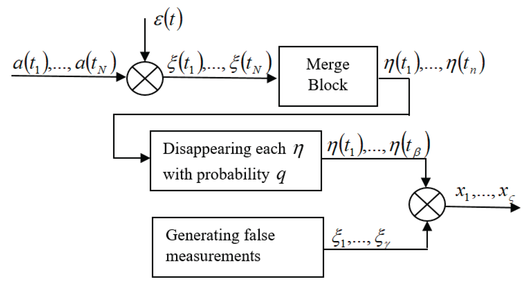
Based on the random nature of all factors of distortion of measurement results in the FC-analyzer, its mathematical model is designed in the form of a conditional probability distribution density of the latter with the specified number and sizes of the measured particles [8]. In Figure 1 schematically shows the process of forming measuring information in the FC-analyzer, taking into account all the noisy factors.

Let the true values of the suspended particle sizes be $r_1,\mathrm{...},r_N$, and the measured values be $x_1,\mathrm{...},x_{\varsigma }$. Due to the merging, disappearance of true values and appearance of false values, the output of the measuring device will contain not $N$ measured values, but $\varsigma$, where $\varsigma =N+\nu -\mu -(\gamma -{\gamma }_1)$, $\nu$ is the number of false measurements; $\mu$ is the number of missing measurements; $\gamma$ is the number of merged measurements; ${\gamma }_1$ is the number of groups obtained as a result of merging.

Let us assume that measurements located close to each other merge with probability $p_{conf}$, which depends on the number of merged points and the distance between them. After merging closely located measurements, one measurement remains with a mathematical expectation equal to the arithmetic mean of the mathematical expectations of the merged measurements. The disappearance of both true measurements and measurements obtained after merging occurs with the same probabilities $q$, i.e. at the output of this block, measurements appear with probability $(1-q)$. Thus, the disappearance occurs according to Bernoulli's law with probability $q$. The appearance of false measurements occurs uniformly, regardless of the merged and missing points. Such an assumption is made for simplicity of reasoning. In fact, the intensity of the appearance of false measurements depends on the location of the true measurements, as well as on their proximity, i.e. in the vicinity after the merger of the obtained measurement there will be a greater number of false measurements.

Let $\varsigma =k$ and be known the value of $(\gamma -{\gamma }_1)=\tilde{\gamma }$. According to the multiplication theorem, it is true

$$p\left(x|r,N\right)=p\left(x|\varsigma =k,r,N\right)\cdot p\left(\varsigma =k|N\right)$$

(1)

Let us calculate the probability

$$p\left(x|\varsigma =k,r,N\right)={\displaystyle \sum _{i}p\left(x|\varsigma =k,\gamma =i,r,N\right)\cdot p\left(\gamma =i|\varsigma =k,N\right)}$$

(2)

Based on the multiplication theorem

$$p\left(\gamma =i|\varsigma =k,N\right)={\displaystyle \frac{p\left(\varsigma =k,\gamma =i|N\right)}{p\left(\varsigma =k|N\right)}}={\displaystyle \frac{p\left(\gamma =i,\mu +\tilde{\gamma }=N+i-k|N\right)}{p\left(\varsigma =k|N\right)}}$$

(3)

Substituting (3) into (2), and the resulting expression into (1), we find

$$\begin{gathered} p\left(x|r,N\right)={\displaystyle \sum _{i}p\left(\nu =i,\mu +\tilde{\gamma }=N=i-k|N\right)\times } \\ \times p\left(x_1,\mathrm{...},x_k|\varsigma =k,\nu =i,r,N\right) \end{gathered}$$

(4)

Let us now define the probability value $p\left(x_1,\mathrm{...},x_k|\varsigma =k,\nu =i,r,N\right)$, where $i$ is the number of false measurements. After the merger and disappearance, $k-i$ true measurements will remain, the total number of different combinations of which, with $N$ actually existing particles, is determined by the number of combinations $C_N^{k-i}$. Taking the disappearance of different combinations as equally probable events, we write

$$\begin{gathered} p\left(x_1,\mathrm{...},x_k|\varsigma =k,\nu =i,r,N\right)={\displaystyle \frac{1}{C_N^{k-i}}}{\displaystyle \sum _{j=1}^{C_N^{k-i}}p\left(x_1,\mathrm{...},x_k|\right.} \\ \left.A_j\equiv \left\{r_{\sigma (j,1)},\mathrm{...},r_{\sigma (j,k-i)}\right\},\varsigma =k,\nu =i,N\right) \end{gathered}$$

(5)

where $A_j\equiv \left\{r_{\sigma (j,1)},\mathrm{...},r_{\sigma (j,k-i)}\right\}$‚ $j=1,\mathrm{...},C_N^{k-i}$, is the set of all possible non-missing combinations. In the index $\sigma \left(j,m\right)$ ($j=1,\mathrm{...},C_N^{k-i},m=1,\mathrm{...},k-i$) $j$ indicates the number in all possible combinations of not missing particles $r$, and $m$ is the number of elements in these combinations.

Of the total number of $k$ elements, $i$ are false; the number of all possible combinations of false elements is $C_k^i$. We consider all these combinations to be equally probable. Let us assume that the last $i$ elements are false, then in $C_k^i$ combinations the elements with numbers $1,2,\mathrm{...},k-i$ will be true, and with numbers $k-i+1,\mathrm{...},k$ will be false. We introduce the general index $s\left(r,l\right)$, $r=1,\mathrm{...},C_k^i$, $l=1,\mathrm{...},k$. When $l=1,\mathrm{...},k-i$, the index $l$ corresponds to true measurements, and when $l=k-i+1,\mathrm{...},k$, to false ones.

According to the above, expression (5) takes the form

$$\begin{gathered} p\left(x_1,\mathrm{...},x_k|\varsigma =k,\nu =i,r,N\right)= \\ ={\displaystyle \frac{1}{C_N^{k-i}}}{\displaystyle \sum _{j=1}^{C_N^{k-i}}\frac{1}{C_k^i}{\displaystyle \sum _{r=1}^{C_k^i}p\left(x_{s(r,1)},\mathrm{...},x_{s(r,k-i)}|x_{\sigma (j,1)},\mathrm{...},x_{\sigma (j,k-i)}\right)\cdot g\left(x_{s(r,k-i+1)}\right)}}\mathrm{...}g\left(x_{s(r,k)}\right)= \\ ={\displaystyle \frac{1}{C_N^{k-i}}}{\displaystyle \sum _{j=1}^{C_N^{k-i}}\frac{1}{C_k^i}{\displaystyle \sum _{r=1}^{C_k^i}\left[{\displaystyle \prod _{t=1}^{i}g\left(x_{s(r,k-i+t)}\right)\cdot p\left(x_{s(r,1)},\mathrm{...},x_{s(r,k-i)}|x_{\sigma (j,1)},\mathrm{...},x_{\sigma (j,k-i)}\right)}\right]}} \end{gathered}$$

(6)

where $g\left(x_{s(r,k-i+t)}\right)$ is the probability of the corresponding measurement being false.

Assuming that the particles in the measuring channel follow randomly and that all possible permutations are equally probable, (6) can be rewritten as follows:

$$\begin{gathered} p\left(x_1,\mathrm{...},x_k|\varsigma =k,\nu =i,r,N\right)= \\ ={\displaystyle \frac{1}{C_N^{k-i}}}{\displaystyle \sum _{j=1}^{C_N^{k-i}}\frac{1}{C_k^i}{\displaystyle \sum _{r=1}^{C_k^i}\left[{\displaystyle \prod _{t=1}^{i}g\left(x_{s(r,k-i+t)}\right)\cdot \frac{1}{\left(k-i\right)!}{\displaystyle \sum _{\mathcal{l}=1}^{\left(k-i\right)!}f\left(x_{s(r,\pi \left(\mathcal{l},m\right))}|r_{\sigma \left(j,m\right)}\right)}}\right.}} \end{gathered}$$

Here $f$ is the distribution density of a single measurement; the index $\pi \left(\mathcal{l},m\right)$ indicates the $m$th permutation in the $\mathcal{l}$th combination.

Let us determine the probability $p\left(\nu =i,\mu +\tilde{\gamma }=N+i-k|N\right)$ from expression (4). According to the multiplication theorem

$$p\left(\nu =i,\mu +\tilde{\gamma }=N+i-k|N\right)=p\left(\nu =i|\mu +\tilde{\gamma }=N+i-k,N\right)\cdot p\left(\mu +\tilde{\gamma }=N+i-k|N\right)$$

(7)

Let us assume that false points appear according to Poisson's law with intensity ${\lambda }_1$ over the time interval $\tau$, i.e.

$$p\left(\nu =i|\mu +\tilde{\gamma }=N+i-k,N\right)={\displaystyle \frac{{\left({\lambda }_1\tau \right)}^i}{i!}}{e}^{-{\lambda }_1\tau }$$

(8)

Probability

$$p\left(\mu +\tilde{\gamma }=N+i-k|N\right)={\displaystyle \sum _{n}p\left(\mu =N+i-k-n|\tilde{\gamma }=n,N\right)\cdot }p\left(\tilde{\gamma }=n|N\right)$$

(9)

We assume that first the merging occurs, then the disappearance of points. The points obtained on the basis of merging may also disappear. In this case, the probability $p\left(\mu =N+i-k-n|\tilde{\gamma },N\right)$ obeys Bernoulli's law with probability $q$, i.e.

$$p\left(\mu =N+i-k-n|\tilde{\gamma },N\right)=C_N^{N+i-k-n}{q}^{N+i-k-n}{\left(1-q\right)}^{k+n-1}$$

(10)

where $p\left(\tilde{\gamma }=n|N\right)$ is the probability that $n+1$ measured values have merged. There are a total of such combinations equal to $C_N^n$. Considering all these combinations to be equally probable, we obtain

$$p\left(\tilde{\gamma }=n|N\right)={\displaystyle \frac{1}{C_N^n}}{\displaystyle \sum _{z=1}^{C_N^n}{p}_{conf}\left(r_{\Im \left(z,1\right)},\mathrm{...},r_{\Im \left(z,n+1\right)}\right)}$$

(11)

where $B_z\equiv \left(r_{\Im \left(z,1\right)},\mathrm{...},r_{\Im \left(z,n+1\right)}\right)$, $z=1,\mathrm{...},C_N^n$, is the set of all possible merged combinations of $n+1$measurements; $z$ is the number of combinations of merged measurements; $n$ is the number of elements in these combinations.

Let us define the summation limits in (9). The expression $\tilde{\gamma }=\gamma -{\gamma }_1=0$ takes place only when no merging occurs, and $\tilde{\gamma }=\gamma -{\gamma }_1=N-1$ when all measurements merge and form one.

Substituting expressions (11) and (10) into (9), taking into account the above, we obtain

$$\begin{gathered} p\left(\mu +\tilde{\gamma }=N+i-k|N\right)={\displaystyle \sum _{n=0}^{N-1}{C}_N^{N+i-k-n}{q}^{N+i-k-n}{\left(1-q\right)}^{k+n-i}\times } \\ \times {\displaystyle \frac{1}{C_N^n}}{\displaystyle \sum _{z=1}^{C_N^n}{p}_{conf}\left(r_{\Im \left(z,1\right)},\mathrm{...},r_{\Im \left(z,n+1\right)}\right)} \end{gathered}$$

(12)

Substitute (12) and (8) into (7). Then

$$\begin{gathered} p\left(\nu =i,\mu +\tilde{\gamma }=N+i-k|N\right)= \\ ={\displaystyle \frac{{\left({\lambda }_1\tau \right)}^i}{i!}}{e}^{-{\lambda }_1\tau }{\displaystyle \sum _{n=0}^{N-1}{C}_N^{N+i-k-n}{q}^{N+i-k-n}{\left(1-q\right)}^{k+n-i}}\times \\ \times {\displaystyle \frac{1}{C_N^n}}{\displaystyle \sum _{z=1}^{C_N^n}{p}_{conf}\left(r_{\Im \left(z,1\right)},\mathrm{...},r_{\Im \left(z,n+1\right)}\right)} \end{gathered}$$

(13)

Taking into account (13) and (8), expression (4) takes the form

$$\begin{gathered} p\left(x|r,N\right)={\displaystyle \sum _i\frac{{\left({\lambda }_1\tau \right)}^i}{i!}{e}^{-{\lambda }_1\tau }{\displaystyle \sum _{n=0}^{N-1}{C}_N^{N+i-k-n}{q}^{N+i-k-n}{\left(1-q\right)}^{k+n-i}}}\times \\ \times {\displaystyle \frac{1}{C_N^n}}{\displaystyle \sum _{z=1}^{C_N^n}{p}_{conf}\left(r_{\Im \left(z,1\right)},\mathrm{...},r_{\Im \left(z,n+1\right)}\right)}{\displaystyle \frac{1}{C_N^{k-i}}}{\displaystyle \sum _{j=1}^{C_N^{k-i}}\frac{1}{C_k^i}\times } \\ \times {\displaystyle \sum _{r=1}^{C_k^i}\left[{\displaystyle \prod _{t=1}^{i}g\left(x_{s(r,k-i+t)}\right)\cdot \frac{1}{\left(k-i\right)!}{\displaystyle \sum _{\mathcal{l}=1}^{\left(k-i\right)!}{\displaystyle \prod _{m=1}^{k-i}f\left(x_{s(r,\pi \left(\mathcal{l},m\right))}|r_{\sigma \left(j,m\right)}\right)}}}\right]}= \\ ={\displaystyle \frac{1}{k!}}{\displaystyle \sum _i\frac{{\left({\lambda }_1\tau \right)}^i}{i!}{e}^{-{\lambda }_1\tau }{\displaystyle \sum _{n=0}^{N-1}{C}_N^{N+i-k-n}{q}^{N+i-k-n}{\left(1-q\right)}^{k+n-i}}}\times \\ \times {\displaystyle \frac{1}{C_N^n}}{\displaystyle \sum _{z=1}^{C_N^n}{p}_{conf}\left(r_{\Im \left(z,1\right)},\mathrm{...},r_{\Im \left(z,n+1\right)}\right)}\times \times {\displaystyle \frac{i}{C_N^{k-i}}}{\displaystyle \sum _{j=1}^{C_N^{k-i}}\frac{1}{C_k^i}{\displaystyle \sum _{r=1}^{C_k^i}\left[{\displaystyle \prod _{t=1}^{i}g\left(x_{s\left(r,k-i+t\right)}\right)\cdot {\displaystyle \sum _{\mathcal{l}=1}^{\left(k-i\right)!}{\displaystyle \prod _{m=1}^{k-i}f\left(x_{s\left(r,\pi \left(\mathcal{l},m\right)\right)}|r_{\sigma \left(j,m\right)}\right)}}}\right]}} \end{gathered}$$

(14)

Let us determine the limits of change of $i$, i.e. the number of false points.

It is obvious that $i\ge 0$, $i\ge k-N$, $i\le k$. Therefore, the final expression (14) can be written as follows:

$$\begin{gathered} p\left(x_1,\mathrm{...},x_k|r,N\right)={\displaystyle \frac{1}{k!}}{\displaystyle \sum _{i=\max \left(0,k-N\right)}\frac{{\left({\lambda }_1\tau \right)}^i}{i!}{e}^{-{\lambda }_1\tau }}\times \\ \times {\displaystyle \sum _{n=0}^{N-1}{C}_N^{N+i-k-n}{q}^{N+i-k-n}{\left(1-q\right)}^{k+n-i}}\times \\ \times {\displaystyle \frac{1}{C_N^n}}{\displaystyle \sum _{z=1}^{C_N^n}{p}_{conf}\left(r_{\Im \left(z,1\right)},\mathrm{...},r_{\Im \left(z,n+1\right)}\right)}\times {\displaystyle \frac{i}{C_N^{k-i}}}{\displaystyle \sum _{j=1}^{C_N^{k-i}}\frac{1}{C_k^i}}\times \\ \times {\displaystyle \sum _{r=1}^{C_k^i}\left[{\displaystyle \prod _{t=1}^{i}g\left(x_{s\left(r,k-i+t\right)}\right)\cdot {\displaystyle \sum _{\mathcal{l}=1}^{\left(k-i\right)!}{\displaystyle \prod _{m=1}^{k-i}f\left(x_{s\left(r,\pi \left(\mathcal{l},m\right)\right)}|r_{\sigma \left(j,m\right)}\right)}}}\right]} \end{gathered}$$

(15)

The probability distribution density of measurement information (15) is obtained taking into account all noisy factors (measurement errors, omitted measurements, occurrence of false measurements, merging of close measurements) with maximum approximation to the real situation.

Expression (15) is extremely cumbersome, and in this form it is practically impossible to use it to estimate the number and sizes of particles suspended in a liquid. Therefore, we formulate a set of conditions under which the expression for the probability distribution density has a comparatively simple form. These conditions cover the indicated noisy factors in a simplified form and reflect the real situation in some idealized form.

The action of noisy factors is described by the following models: true measurements form a Poisson flow with intensity $\lambda$ over time $\tau$, where $\tau$ is the length of the section on the time axis containing all the measurements of interest to us; errors in measuring particle sizes are assumed to be additive normal with zero mathematical expectations and with variance ${\sigma }^2$; missing measurements occur independently for each single measurement with probability $p_{admi}$; false measurements form a Poisson flow with intensity ${\lambda }_1$ over time $\tau$, where ${\lambda }_1<<\lambda$, the non-resolution is described by the probability of obtaining one measurement for two particles, the time distance $\Delta t$ between which satisfies the inequality $\Delta t\le {\Delta }_t$, i.e. the merging of measurements from two particles depends not on the moment of their passage into the working zone, but on the distance between them.

Given the fact that true measurements form a Poisson flow with intensity $\lambda$, the probability of merging measurements from two particles is equal to the probability that two particles appear in the measurement zone during the time $\Delta t$, i.e.

$$p_{conf}=P\left(\xi =2|{\Delta }_t\right)={\displaystyle \frac{{\left(\lambda {\Delta }_t\right)}^2}{2!}}{e}^{-\lambda {\Delta }_t}$$

After the merging of two measurements, the moments of appearance of the resulting measurement and the first particle coincide, the mathematical expectation of the unresolved signal is equal to $f\left(r_i,r_{i-1}\right)$, and the variance is ${\sigma }_c^2$.

Let us formulate the conditions under which the probability distribution density of the flow is sought. At the output of the measuring channel there is a set of $\varsigma$ measurements $\left(x_1,\mathrm{...},x_{\varsigma }\right)$ obtained in the presence $N$ of particles with sizes $\left(r_1,\mathrm{...},r_N\right)$. At the same time: 1) the measurements are far from each other, i.e. $\left|t_i-t_j\right|>{\Delta }_t$, $i\ne j$, $i,j=1,\mathrm{...},\varsigma$ (this assumption is close to reality if the non-resolution threshold of the measuring device is less than the interval between neighboring particles); 2) in the vicinity of each measurement either there are no particles, i.e. the measurement is false, or there is one particle, then the measurement corresponds to an existing particle, or there are two particles, then the measurement is obtained from an unresolved group of two particles; 3) in areas where there are no measurements, there are no groups of two or more particles. The last condition means, in particular, that a measurement can be missed only for a single particle, and a group of two sufficiently close particles necessarily gives a measurement, which apparently corresponds to reality. As follows from these conditions, groups of three or more particles are not taken into account.

Let us assume that there are $k_1$ situations satisfying the condition of having true measurements, $k_2$ situations satisfying the condition of having merged measurements, $k_3=\varsigma -k_1-k_2$ situations satisfying the condition of having false measurements, $k_4=N-k_1-2k_2$ situations satisfying the condition of having missing measurements. Then the probability distribution density of measurements can be approximately represented as follows

$$\begin{gathered} p\left(x_1,\mathrm{...},x_{\varsigma }|r_1,\mathrm{...},r_N\right)\approx {\left(1-p_{pass}\right)}^{k_1}{\displaystyle \frac{{\left(\lambda \tau \right)}^{k_1}}{k_1!}}{e}^{-\lambda \tau }\times \\ \times {\displaystyle \prod _{i=1}^{k_1}\frac{1}{\sqrt{2\pi }\sigma }\exp \left\{-\frac{{\left(x_i-r_i\right)}^2}{2{\sigma }^2}\right\}{\displaystyle \prod _{\mathcal{l}=1}^{k_2}\frac{{\left(\lambda {\Delta }_t\right)}^2}{2!}{e}^{-\lambda {\Delta }_t}\frac{1}{\sqrt{2\pi }{\sigma }_c}}}\times \\ \times \exp \left\{-{\displaystyle \frac{1}{2{\sigma }_c^2}}{\left(x_{\mathcal{l}}-{\displaystyle \frac{r_{2\mathcal{l}-1}+r_{2\mathcal{l}}}{2}}\right)}^2\right\}{\displaystyle \frac{{\left({\lambda }_1\tau \right)}^{k_3}}{k_3!}}{e}^{-{\lambda }_1\tau }{\displaystyle \prod _{s=1}^{k_4=N-k_1-2k_2}{p}_{miss}} \end{gathered}$$

(16)

where $p_{miss}$ is the probability of the measured value disappearing.

The expression (16) is also very complicated, its use to assess the number and dimensions of particles suspended in the liquid requires the use of a powerful computing technology. Therefore, we will take the next step along the path of simplifying the task. We will solve it in two stages. At the first stage, based on measuring information obtained in $M$ measuring channels, we will estimate the true number of particles in the time interval $\tau$, and on the second stage, independently of each other, we will estimate the true size of the particles according to the registered values in the $M$ channels.

The probability distribution density of the registered number of particles in the $i$th measurement channel ($i=1,\mathrm{...},M$) for the time interval $\tau$ is determined as follows:

$$\begin{gathered} p\left(\varsigma =N_i|N\right)={\left(1-p_{pass}\right)}^{k_1}{\displaystyle \frac{{\left(\lambda \tau \right)}^{k_1}}{k_1!}}{e}^{-\lambda \tau }{\displaystyle \prod _{\mathcal{l}=1}^{k_2}\frac{{\left(\lambda {\Delta }_t\right)}^2}{2!}{e}^{-\lambda {\Delta }_t}\times } \\ \times {\displaystyle \frac{{\left({\lambda }_1\tau \right)}^{k_3=N_i-k_1-k_2}}{k_3!}}{e}^{-{\lambda }_1\tau }{\displaystyle \prod _{s=1}^{k_4=N-k_1-2k_2}{p}_{miss}} \end{gathered}$$

(17)

Suppose that measurements in each channel are carried out independently of each other and all the noisy factors in each channel also act independently of each other. Then the estimates for $k_1$, $k_2$, $k_3$, $k_4$ can be found by maximizing the probability distribution density (17), that is, by solving a fairly simple problem

$$\underset{\left\{k_1,k_2,N\right\}}{\max }\left\{{\displaystyle \prod _{i=1}^{M}P\left(\varsigma =N_i|N\right)}\right\}$$

where $k_1\in R_1$, $k_2\in R_2$, $N\in R_0$, $R_0$, $R_1$, $R_2$ are the given sets of positive integers.

Let us now consider the process of registering the true measurements and assessment of the dimensions of particles suspended in the liquid based on $M$-channel meter. We accept that the registration of particles is carried out using $M$ photo-registers that receive light signals either from one light source through one counting zone, or from $M$ light sources installed along the channel of the course of the analyzed liquid and acting the same type. In the first case, the registration of the same particle in all receivers is carried out at the same time, in the second - there will be known temporary shifts between them, which can always be compensated and measurements from the same particles to perceive as received in all receivers at the same moment.

In each measurement channel, a random number of measurements are obtained at random times. It is obvious that true measurements related to the same particle in all channels appear at the same time. Since we assume that the noise factors in each channel act independently of each other, it is obvious that false measurements in different channels will appear with a higher probability at different times, and measurements will also disappear and merge at different times.

Based on the above, we will construct the following algorithm for registering true measurements and estimating particle sizes. Let measurements ${\varsigma }_j$ ($0\le {\varsigma }_j\le M$) be registered in $M$ channels at a given time $t_j$. It is necessary to decide whether these measurements are false and should be ignored or whether most of them are true and it is necessary to estimate particle sizes based on them. Since the probability that false measurements appear in all channels at the same time is small, and the probability of missing measurements in all channels at the same time is also insignificant, we choose the following decision rule: if

$$\gamma \le {\varsigma }_j$$

(18)

then a decision is made that the measurements in the channels are obtained from a suspended particle, otherwise, that the measurements are false ($0\le \gamma <M$). The threshold $\gamma$ is chosen so that

$$P\left(\gamma \le {\varsigma }_j|r\right)=1-\alpha$$

(19)

where the condition in probability indicates the presence of a suspended particle.

To determine $\gamma$, we find the distribution density of the random variable ${\varsigma }_j$. If there is a particle in the counting zone, we have ${\varsigma }_j=M-{\mu }_j-{\beta }_j$, where ${\beta }_j$ is the number of missing measurements due to merging with the measurement from a neighboring particle; ${\mu }_j$ is the number of missing measurements in the absence of a particle in the counting zone. In the latter case, ${\varsigma }_j={\nu }_j$, where ${\nu }_j$ is the number of false measurements in $M$ channels.

If it is necessary not to overestimate the concentration of suspended particles in a liquid, we select the decision rule as follows:

$$\underset{\left\{\gamma \right\}}{\max }P\left(\gamma \le {\varsigma }_j|r\right)$$

(20)

given that

$$P\left(\gamma \le {\varsigma }_j|0\right)\le \alpha$$

(21)

Otherwise, we solve the problem

$$\underset{\left\{\gamma \right\}}{\min }P\left(\gamma \le {\varsigma }_j|0\right)$$

(22)

given that

$$P\left(\gamma \le {\varsigma }_j|r\right)\ge 1-\alpha$$

(23)

To solve the problem (20), (21) or (22), (23) it is necessary to find the probability distribution densities $p\left({\varsigma }_j|r\right)$ and $p\left({\varsigma }_j|0\right)$. Let the probability of a false measurement appearing in the $i$th channel be equal to $p_{false}^i$. Then the probability that at $t_j$ moment of time a false measurement appeared in ${\nu }_j$ channels is equal to ${\displaystyle \prod _{i=1}^{{\nu }_j}{p}_{false}^i}$ and condition (21) takes the form

$$P\left(\gamma \le {\varsigma }_j|0\right)={\displaystyle \sum _{{\nu }_j=\gamma }^M{\displaystyle \prod _{i=1}^{{\nu }_j}{p}_{false}^i}}\le \alpha$$

(24)

Obviously, condition (24) is not satisfied for any values of $p_{false}^i$ and $\alpha$. This means that for different $p_{false}^i$ the limits of the achievable quality of non-registration of false measurements are different. Therefore, based on the value $\alpha$ in different channels of registration of suspended particles, it is necessary to select the thresholds for registering signals in such a way that condition (21) is satisfied.

Let us assume that the loss of a measurement in the $i$th channel due to merging can only occur by merging this measurement with the closest one in time, i.e.

$$p_{conf}^i={\displaystyle \frac{{\left(\lambda {\Delta }_t^i\right)}^2}{2!}}{e}^{-\lambda {\Delta }_t^i},$$

and the probability of each dimension being missing is the same and equal to $p_{miss}$. According to the multiplication theorem

$$P\left({\varsigma }_j=n_j|M\right)={\displaystyle \frac{1}{M-n_j+1}}{\displaystyle \sum _{k_j=0}^{M-n_j}P\left({\varsigma }_j=n_j|{\mu }_j=k_j,M\right)P\left({\mu }_j=k_j|M\right)}$$

(25)

$$P\left({\mu }_j=k_j|M\right)=C_{M-n_j}^{k_j}{p}_{miss}^{k_j}{\left(1-p_{miss}\right)}^{M-n_j-k_j},0\le k_j\le M-n_j$$

(26)

$$\begin{gathered} P\left({\varsigma }_j=n_j|{\mu }_j=k_j,M\right)=P\left({\varsigma }_j=n_j|{\mu }_j=k_j,\beta =M-k_j-n_j,M\right)\times \\ \times P\left({\beta }_j=M-k_j-n_j|M\right) \\ P\left({\beta }_j=M-k_j-n_j|M\right)={\displaystyle \frac{1}{C_{M-n_j}^{M-k_j-n_j}}}{\displaystyle \sum _{\mathcal{l}=1}^{C_{M-n_j}^{M-k_j-n_j}}{\displaystyle \prod _{p=1}^{M-k_j-n_j}{p}_{conf.\Im \left(\mathcal{l},p\right)}}}; \end{gathered}$$

(27)

where the index $\Im \left(\mathcal{l},p\right)$ indicates the $p$th permutation in the $\mathcal{l}$th combination. After receiving $n_j$ measurements in $M$ channels at the moment of time $t_j$, it is true

$$P\left({\varsigma }_j=n_j|{\mu }_j=k_j,\beta =M-k_j-n_j,M\right)=1$$

(28)

Taking into account (26) - (28), expression (25) takes the form

$$\begin{gathered} P\left({\varsigma }_j=n_j|M\right)={\displaystyle \frac{1}{M-n_j+1}}{\displaystyle \sum _{k_j=0}^{M-n_j}\left\{C_{M-n_j}^{k_j}\right.p_{miss}^{k_j}{\left(1-p_{miss}\right)}^{M-n_j-k_j}\times } \\ \left.\times {\displaystyle \frac{1}{C_{M-n_j}^{M-k_j-n_j}}}{\displaystyle \sum _{\mathcal{l}=1}^{C_{M-n_j}^{M-k_j-n_j}}{\displaystyle \prod _{p=1}^{M-k_j-n_j}{p}_{conf.\Im \left(\mathcal{l},p\right)}}}\right\}, \end{gathered}$$

(29)

and taking into account (29), condition (23) will be written as follows:

$$\begin{gathered} P\left(\gamma \le {\varsigma }_j|r\right)={\displaystyle \sum _{n_j=\gamma }^M\frac{1}{M-n_j+1}{\displaystyle \sum _{k_j=0}^{M-n_j}\left\{C_{M-n_j}^{k_j}\right.p_{miss}^{k_j}{\left(1-p_{miss}\right)}^{M-n_j-k_j}\times }} \\ \left.\times {\displaystyle \frac{1}{C_{M-n_j}^{M-k_j-n_j}}}{\displaystyle \sum _{\mathcal{l}=1}^{C_{M-n_j}^{M-k_j-n_j}}{\displaystyle \prod _{p=1}^{M-k_j-n_j}{p}_{conf.\Im \left(\mathcal{l},p\right)}}}\right\}\ge 1-\alpha \end{gathered}$$

(30)

Similar to condition (24), inequality (30) is not satisfied for any values of $p_{miss}$, $p_{conf}$ and $\left(1-\alpha \right)$. This means that for given $p_{miss}$ and $p_{conf}$ it is impossible to achieve any quality of measurement. Therefore, it is necessary to select such characteristics of the measurement channels that the corresponding values of $p_{miss}$ and $p_{conf}$ satisfy (30). Expressions that allow us to calculate $p_{false}$, $p_{miss}$ and $p_{conf}$ for a single-channel FC-analyzer are given below.

Thus, rule (18), where $\gamma$ is defined as stated above, makes it possible to make a decision regarding the presence of a particle in the counting zone at a time $t_j$. Let us denote the measurement result in the $i$th channel at a time $t_j$ by $x_i\left(t_j\right)$. Two approaches are possible to estimate the true size of this particle: the first is averaging all the measurements obtained

$${\widehat{r}}_j={\displaystyle \frac{1}{{\varsigma }_j}}{\displaystyle \sum _{i=1}^{{\varsigma }_j}{x}_i\left(t_j\right)}$$

(31)

the second - under the assumption that true measurements form a compact group, and false ones are likely to be removed from the center of the compact group; we use formula (31) only for measurements from this compact group.

Thus, for a joint assessment of the number and size of particles suspended in a liquid, several (more than one) measuring channels are required. Developing an optimal algorithm for such an assessment, taking into account all the noise factors, is a practically unsolvable problem. Constructing a quasi-optimal estimate of the number of true measurements in a given time interval based on measurement information obtained in one measuring channel is feasible, but requires the use of powerful computing equipment. The construction of an optimal decision rule that makes it possible, based on the measurement information obtained in $M$ ($M>1$) channels, regardless of the information at other times, to detect the presence of a particle in the measurement zone and determine its size is not difficult. Its implementation is possible on the basis of microprocessor technology.

3. Simulation model of the analyzer of mechanical impurities in a liquid medium

The purpose of mathematical models of measuring instruments is to minimize the material and time costs of their development, as opposed to natural modeling. At the same time, achieving a global optimum in the task of optimizing the device in the first case is quite possible, while in the second case it is practically unrealizable in the foreseeable future due to the large number of decision-making options. Therefore, when developing mathematical models, it is necessary to strive to make them as simple, compact, and clear as possible, and at the same time to correspond as much as possible to the real processes occurring in the phenomena under study.

It is obvious that due to their bulkiness and complexity, expressions (15), (17) are unsuitable for estimating the number and size of suspended particles in a liquid. In addition, they do not include the technical characteristics of the device (structural, optical, electrical, etc.), so they cannot be used for optimal design of the device.

To eliminate the noted shortcomings, simulation models of the analyzer under consideration have been developed, in which the operation of individual units and their interrelationship are simulated based on formalized regularities. These regularities include the technical characteristics of the analyzer as parameters. The latter allows one to formulate and solve the problem of optimizing the methodological and technical solutions implemented in the device, using the measure of discrepancy between the laws of particle size distribution in the analyzed medium and at the device output as an optimization criterion.

Depending on the given law of probability distribution of sizes (diameters) of particles analyzed in a liquid medium $p_2\left(x\right)$, the optimal value of the number of fractions $L$ and the average values of diameters for each fraction $d_i$ are calculated. Then, a Poisson flow of true particles is generated with the parameter $\lambda T$, where $T$ is the duration of the analysis, $\lambda$ is the intensity of the Poisson flow, depending on the concentration of particles in the analyzed medium and the velocity of the liquid flow through the counting zone, determined on the basis of experimental data for a specific medium; the total number of true particles $n_0$, the number of particles $n_i$ that fall into the $i$th fraction, and, of course, the frequency of particles falling into the $i$th fraction $k_i=n_i/n_0$ are calculated.

For given <!-- MathType@Translator@5@5@MathML2 (no namespace).tdl@MathML 2.0 (no namespace)@ -->

$d_{\min }$, and probability $p$, according to [9], $V_{CZ}=p\cdot {10}^{-m}/n\left(a\right)$ is determined, where $n_{\max }=n\left(a\right)\cdot {10}^m$, $1<n\left(a\right)<10$, $Q=V_{CZ}/\left(1.7{\tau }_{\min }\right)$. Here $n_{\max }$ is the maximum possible number of particles registered in the CZ during time $T$; $d_{\min }$ is the minimum possible particle diameter; ${\tau }_{\min }$ is the minimum signal duration, which is selected from the boundary conditions imposed by the electronic circuit; $V_{CZ}$ is the volume of the CZ; $Q$ is the volumetric flow rate.

Assuming that the liquid flow channel is quadratic, from the condition $8abh\le V_{CZ}$, $4bh\le S_{CZ}$, we calculate $2h$, where $a$, $b$ and $h$ are the width, length, and height of the CZ of a channel, respectively; $S_{CZ}$ is the CZ area determined from the condition $k_{\min }^m\ge S\left(d_{\min }\right)/S_{CZ}=0.001$; $S\left(d_{\min }\right)$ is the area corresponding to the minimum diameter of a particle suspended in the liquid. Next, we calculate the “dead time” value ${\tau }_{DT}$, i.e. the time during which, after a particle passes through the CZ, the photodetector does not respond to the signal of the next particle, ${\tau }_{DT}=\left(1-{\displaystyle \frac{E_D}{2u}}\right){\tau }_{im}$, where ${\tau }_{im}$ is the duration of the impulse, which can be recalculated from its amplitude and shape; $u$ is the impulse amplitude, $u\equiv S\left(d\right)$; $E_D$ is the level of discrimination, $E_D\equiv S\left(d_{\mathrm{thr}}\right)$ ($d_{\mathrm{thr}}$ is the threshold value of the diameter). The volume of the $j$th particle is $V_j=Q{\tau }_{DT}$. Taking into account $d_i^2\approx u_i$, a value $d_{\mathrm{thr}}$ is selected depending on the noise level in the electrical circuit based on the ratio

$$P\left(d_{\mathrm{i}}\le d_{\mathrm{thr}}\right)=p_{\mathrm{thr}}.$$

For the given value $d_{\mathrm{thr}}$, due to random fluctuations in the electrical circuit, false measurements may occur, i.e.

$$P\left(u_{false}>u\left(d_{\mathrm{thr}}\right)\right)=p_{\mathrm{false}}.$$

(32)

Assuming that in the electrical scheme there is white noise with variance ${\sigma }_{fl}^2$, (32) is rewritten in the form

$$p_{false}={\displaystyle \underset{u\left(d_{thr}\right)}{\overset{+\infty }{\int }}\frac{1}{\sqrt{2\pi }{\sigma }_{fl}}}{e}^{-{\displaystyle \frac{x^2}{{\sigma }_{fl}^2}}}dx=1-\Phi \left({\displaystyle \frac{u\left(d_{thr}\right)}{{\sigma }_{fl}}}\right).$$

For a given ${\sigma }_{fl}$ by the choice of $d_{\mathrm{thr}}$, the probability value $p_{\mathrm{false}}$ can be made arbitrarily small. The value $d_{\mathrm{thr}}$ must be chosen so that it holds $p_{\mathrm{miss}}\to \min$ for $p_{\mathrm{false}}\le \alpha$, where $p_{\mathrm{miss}}$ is calculated [9]:

$$\begin{gathered} p_{\mathrm{miss}}={\displaystyle \frac{{\left(n_0{V}_{CZ}\right)}^2}{4}}{\displaystyle \sum _{j=1}^L{k}_j{\displaystyle \sum _{i=1}^L{k}_i\left(1+\frac{\sqrt{d_i^2-d_{thr}^2}}{2h}\right)}}\times \\ \times {\displaystyle \frac{Q{\tau }_{DT}}{V_{CZ}}}\exp \left[-k_i{n}_0{V}_{CZ}\left(1+{\displaystyle \frac{\sqrt{d_i^2-d_{thr}^2}}{2h}}\right)\right]. \end{gathered}$$

The probability of merging measurements from different particles in the analyzer under consideration is determined by the relation $p_{conf}=p_{c1}+p_{c2}$, where

$$\begin{gathered} p_{\mathrm{c}1}={\displaystyle \frac{{\left(n_0{V}_{CZ}\right)}^2}{4}}{{\displaystyle \sum _{j=1}^L{k}_j{\displaystyle \sum _{i=1}^L{k}_i\left(1+\frac{\sqrt{d_i^2-d_{thr}^2}}{2h}\right)}}}^2\times \\ \times \exp \left[-k_i{n}_0{V}_{CZ}\left(1+{\displaystyle \frac{\sqrt{d_i^2-d_{thr}^2}}{2h}}\right)\right] \\ {p}_{\mathrm{c}2}={\displaystyle \frac{{\left(n_0{V}_{CZ}\right)}^2}{4}}{\displaystyle \sum _{i=1}^L{\displaystyle \sum _{j=1}^L{k}_i{k}_j\left(1+\frac{\sqrt{d_i^2-d_{thr}^2}}{2h}\right)}}{\displaystyle \frac{k\sqrt{d_i^2-d_{thr}^2}}{2h}}\times \\ \times \exp \left[-k_i{n}_0{V}_{CZ}\left(1+{\displaystyle \frac{\sqrt{d_i^2-d_{thr}^2}}{2h}}\right)\right]; \end{gathered}$$

merging threshold ${\Delta }_{\mathrm{t}}$ is determined by ratio

$$P\left(\left|t_{\mathrm{i}}-t_{\mathrm{i}+1}\right|\le {\Delta }_{\mathrm{t}}\right)=p_{\mathrm{conf}}.$$

(33)

Assuming that more than one particle can appear in the CZ for ${\Delta }_{\mathrm{t}}$, which form a Poisson flow, we can write

$$P\left(\left|t_{\mathrm{i}}-t_{\mathrm{i}+1}\right|\le {\Delta }_{\mathrm{t}}\right)={\displaystyle \sum _{k=2}^{\infty }\frac{{\left(\lambda {\Delta }_{\mathrm{t}}\right)}^k}{k!}e{}_{-\lambda {\Delta }_{\mathrm{t}}}}=1-{\displaystyle \sum _{k=0}^1\frac{{\left(\lambda {\Delta }_{\mathrm{t}}\right)}^k}{k!}e{}_{-\lambda {\Delta }_{\mathrm{t}}}}.$$

In this case, equation (33), solved with respect to ${\Delta }_{\mathrm{t}}$, is rewritten as follows:

$$1-p_{conf}=e^{-\lambda {\Delta }_{\mathrm{t}}}\left(1+\lambda {\Delta }_{\mathrm{t}}\right).$$

The diameter of the particle that appears as a result of merging two other particles at moments in time $t_{\mathrm{i}}$ and $t_{\mathrm{i}+1}$ is determined by the dependence $f\left(d_{\mathrm{i}},d_{\mathrm{i}+1}\right)$.

The intensity of false measurements is determined depending on the concentration of interfering components in the studied medium (gas bubbles, photodiode noise impulses, etc.). Multiple experimental data confirm that the distribution of photodiode noise impulses by amplitude obeys the normal law, and in time - the Poisson law [10].

The intensity of noise impulses is determined by the formula ${\lambda }_1={\lambda }_{\mathrm{ns}}=N_{\mathrm{ns}}/t_{\mathrm{ns}}$, where $N_{\mathrm{ns}}$ is the number of registered noise signal impulses; $t_{\mathrm{ns}}$ is the time of measuring the intensity of noise impulses. The variance of the amplitudes of noise impulses is determined by experimental data [10].

The simulation of the process of formation of measurement information in the analyzer is carried out according to the following algorithm. In a given time interval $\left[0,T\right]$, a Poisson flow with intensity $\lambda$ is simulated, i.e. random moments of time $0<t_1<t_2<t_3<\mathrm{...}<t_{\mathrm{N}}\le T$ are determined, at which particles suspended in a liquid medium are measured. The probability distribution density of the Poisson flow is denoted by $p_1\left(\lambda ,T\right)$. The sizes of suspended particles are simulated according to a given law $p_2\left(x\right)$. For example, with the normality of this law $p_2\left(x\right)=N\left(x;a,{\sigma }^2\right)$, where $a$ is the mathematical expectation of the sizes of suspended particles, ${\sigma }^2$ is the variance of these sizes.

Particles that appear at adjacent moments of time $t_{\mathrm{i}}$, $t_{\mathrm{i}+1}$ and for which the condition $\left|t_{\mathrm{i}}-t_{\mathrm{i}+1}\right|\le {\Delta }_{\mathrm{t}}$ is satisfied merge: instead of two particles, one is simulated at the moment of time $t_{\mathrm{i}}$ with diameter $f\left(d_{\mathrm{i}},d_{\mathrm{i}+1}\right)$. The diameters of the simulated particles $d_{\mathrm{j}}$ are compared with the threshold value $d_{\mathrm{thr}}$ and particles for which $d_{\mathrm{j}}\le d_{\mathrm{thr}}$ disappear, i.e., the measurement disappears at the corresponding moment of time $t_{\mathrm{j}}$.

In the time interval $\left[0,T\right]$, a Poisson flow of false measurements with intensity ${\lambda }_1$ is modeled: random moments of time $0<t_1^{*}<t_2^{*}<\mathrm{...}<t_{\nu }^{*}\le T$ are determined at which false measurements appear. We denote the probability density of this flow by $p_3\left({\lambda }_1,T\right)$. Impulses from false measurements are modeled according to the law $p_4\left(x\right)$. In cases where $\left|t_{\mathrm{i}}-t_j^{*}\right|\le {\Delta }_{\mathrm{t}}$, instead of two measurements, one true and one false, there remains one measurement at the time $t_{\mathrm{i}}$ with the value $f\left(d_{\mathrm{i}},d_j\right)$.

When modeling the intensity of Poisson flows ${\lambda }_1$ and ${\lambda }_2$, the values of thresholds ${\Delta }_{\mathrm{t}}$ and $d_{\mathrm{thr}}$, the distribution parameters $p_2\left(x\right)$ and $p_4\left(x\right)$, the values of probabilities $p_{\mathrm{conf}}$, $p_{\mathrm{miss}}$ and $p_{\mathrm{false}}$ are set as described above.

4. Optimization of the structure and parameters of the mechanical impurity analyzer according to the developed models

One of the main goals of developing a simulation model of an analyzer is to optimize the methodological and technical solutions adopted in the device. In this case, the measure of the discrepancy between the probability distribution laws of particle sizes in the analyzed medium and at the device output can be used as an optimization criterion. Let us denote by $p_{\mathrm{i}}$ ($i=1,\mathrm{...},L$) the probability of particles getting into the $i$th fraction of the analyzed medium, and by $p_i^{*}$ - the frequency of getting the obtained (measured) values into the $i$th fraction at the output of the simulation model of the device; $L$ is the number of fractions. Then, as an optimization criterion for the device, we take

$$\min \left\{{\displaystyle \sum _{i=1}^L\left(p_i-p_i^{*}\right)}\right\}$$

(34)

when the following conditions are met:

$$p_{\mathrm{miss}}\to \min ,p_{\mathrm{false}}\le \alpha ,p_{\mathrm{conf}}\le \beta ,$$

(35)

where $\alpha$ and $\beta$ are given probabilities.

Probabilities $p_i^{*}$, $p_{\mathrm{miss}}$, $p_{\mathrm{false}}$, $p_{\mathrm{conf}}$ depend on the methodological and technical decisions taken in the device, such as design decisions (dimensions of the measuring cuvette, shape and location of the sample preparation and feeding unit), intensity of the light source, sensitivity of the photodetector, etc. Let us denote the set of design parameters by $\omega$; characteristics of the analyzed medium (probability distribution function of particle sizes in the analyzed medium) - by $\theta$; noise characteristics of the device (fluctuations of the light source and photodiode, auto-fluctuation of the measurement channels, intensity of occurrence of false measurements) - through $\eta$, methodological solutions (the value of the filtering threshold of the electrical signal, the shape of the measuring cuvette, the shape of the light source, the shape of the counting zone, etc.) - through $\delta$, and through ${\Omega }_{\omega }$, ${\Omega }_{\theta }$, ${\Omega }_{\eta }$, ${\Omega }_{\delta }$ - the areas of permissible values, respectively, of the design characteristics of the analyzed medium, the noise characteristics of the device and methodological solutions. Then problem (34), (35) must be solved under the following restrictions:

$$\omega \in {\Omega }_{\omega }$$

(36)

In general, the problem (33) - (36) is multidimensional and nonlinear. The development of convergent methods for its solution largely depends on the characteristics of existing dependencies between different parameters. As a rule, the development and study of such methods is a very complex task, requiring large material and time costs. Its solution is significantly simplified by simulation modeling. In this case, for admissible values of parameters $\omega$, $\theta$, $\eta$, $\delta$ the frequencies $p_i^{*}$, $i=1,\mathrm{...},L$, are modeled and those values of the parameters that correspond to the minimum value of criterion (34) are selected. If there are several solutions, the more technologically advanced, simple to implement, economical, etc. solution is preferable. It is essential to reduce the number of possible enumerations of the values of the parameters under consideration. This is achieved using combinatorics methods and various logical considerations, taking into account the existing interrelations between the parameters under consideration.

5. Conclusions

Mathematical and simulation models of the analyzer of mechanical impurities in a liquid medium have been developed, which are used to optimize the structure of measuring instruments with a built-in microprocessor, optimal selection of parameters and algorithms for processing and filtering information, which guarantees high quality of measurement. These models are used at the design stage to optimize the structure and parameters of the designed instrument in order to improve its metrological characteristics. At the same time, the funds and time required to develop high-quality auto analyzers are significantly reduced. Algorithms for parametric optimization of measuring instruments based on their mathematical models, optimization of the structure and parameters of the analyzer of mechanical impurities according to the developed models are proposed.

References

- Primak A.V., Kafarov V.V. and Kachiashvili K.J. System Analysis of Air and Water Quality Control. Naukova Dumka, Kiev, 1991, p. 358.
- Schiering N., Eichstädt S., Heizmann M., Koch W., Schneider L. S., Scheele S. and Sommer K. D. Modelling of measuring systems – From white box models to cognitive approaches. Measurement: Sensors 2024, 1-10. [CrossRef]
- Lazarev I.A. Compositional modeling of complex aggregate systems. Radio and Communications, Moscow, 1986, p. 311.
- Sommer K.-D., Harris P., EichstЁadt S., Füssl R., Dorst T., Schütze A., Heizmann M., Schiering N., Maier A., Luo Y., Tachtatzis C., Andonovic I., Gourlay G. Modelling of networked measuring systems – from white-box models to data based approaches, 2023, 1-39. arXiv:2312.13744.
- Heizmann M., Leon F. P. Modellbildung in der Mess- und Automatisierungstechnik, TM - Tech. Mess, Volume 83(2), 63–65. [CrossRef]
- Sommer K.D., Kochsiek M., Siebert B. R.L., Weckenmann A. A Generalized Procedure for Modelling of Measurement for Evaluating the Measurement Uncertainty. Proceedings IMEKO and CMS (ISBN 953-7124-00-2) 17th IMEKO WORLD CONGRESS, Dubrovnik, 2003.
- Sommer K. D., Weckenmann A. and Siebert B. R. L. A systematic approach to the modelling of measurements for uncertainty evaluation. Journal of Physics: Conference Series 13, 7th International Symposium on Measurement Technology and Intelligent Instruments, 2005, 224–227.
- International Organization for Standardization (ISO) 1993 first edition 1993 corrected and reprinted, 1995, Guide to the Expression of Uncertainty in Measurement (GUM), Geneva.
- Mesropyan E.A. Photometric-counting method for determining the size of suspension particles with automated calibration. Thesis for the degree of candidate of technical sciences. Moscow, 1984.
- Study of the properties of the dispersed composition of mechanical impurities in AMG-10 oil for the purpose of optimally matching the parameters of the suspension analyzer type AC-110. Supervisor: Karabegov M.A., VNIIAT report on research, vol. 1204, 1976, Tbilisi.
Figure 1.
The block diagram of the process of the formation of measuring information in the FC-analyzer of mechanical impurities with the noisy factors.
Disclaimer/Publisher’s Note: The statements, opinions and data contained in all publications are solely those of the individual author(s) and contributor(s) and not of MDPI and/or the editor(s). MDPI and/or the editor(s) disclaim responsibility for any injury to people or property resulting from any ideas, methods, instructions or products referred to in the content. |
© 2025 by the authors. Licensee MDPI, Basel, Switzerland. This article is an open access article distributed under the terms and conditions of the Creative Commons Attribution (CC BY) license (http://creativecommons.org/licenses/by/4.0/).
Copyright: This open access article is published under a Creative Commons CC BY 4.0 license, which permit the free download, distribution, and reuse, provided that the author and preprint are cited in any reuse.