
Submitted:
05 June 2025
Posted:
05 June 2025
You are already at the latest version
Abstract
In this research we address the problem of background subtraction using a parallel algorithm implemented and tested on GPU processors and compare our findings with the state-of-the-art. Our results demonstrate that our algorithm achieves a high number of processed frames per second while maintaining output quality equivalent to leading-edge algorithms. Background subtraction has applications in many areas, ranging from automotive and tool inspection to object detection, recognition, and tracking. While current algorithms commonly rely on mixture of Gaussian models, our algorithm is trained with a small set of sample frames, modeling pixels with lognormal distributions. During the testing phase, we compare pixel intensities with the lognormally distributed values from training with the view to infer a probabilistic score, which classifies each pixel as either foreground or background.
Keywords:
background subtraction
; parallel algorithms
; GPU processing
; log-normal distribution
1. Introduction
Since its inception background subtraction has always been an interesting problem among computer vision researchers. Background subtraction is the computer vision technique where the background is removed from the foreground. Foreground is the cluster of pixels that denote a moving object in the scene, captured by a camera, which is separated and distinguished from the background. This segmentation of pixels between foreground and background has been important, with many applications, in several areas ranging from medical imaging, astronomy, machine vision and tool inspection to action recognition and, vehicle detection and tracking [1]. The advent of autonomous vehicles has caused a resurgence of interest in the background subtraction techniques for detecting moving vehicles, pedestrians, animals, and other objects of interest [2]. Even though background subtraction is a well-studied problem, many challenges remain open and unsolved. In particular, dynamic scenes that include several moving objects, changes in illumination conditions, shadows, occluded objects or foreground objects that become part of the background, when, for instance, a moving vehicle is stopped or parked, make background subtraction a difficult yet a challenging problem.
A basic technique to tackle the problem of background subtraction is through pixel differencing, that is, subtracting corresponding pixels between two consecutive image frames while a given threshold differentiates between foreground and background pixels. The resulting, black and white, image provides a representation of the pixels belonging to either one of the two categories. Complex environments, however, require more sophisticated methods to deal with noise, shadows, changes in illumination conditions, and a time interval to consider a pixel as a background or foreground. A significant number of background subtraction algorithms rely on statistical techniques to tackle the aforementioned issues, for example, mixture of Gaussians [3] or optical flow [4] where the motion parameters of pixels are inferred with respect to time and space, thus allowing the segmentation of pixels belonging to multiple foreground objects.
In this research, the problem of background subtraction is addressed using statistical techniques that model pixel intensities with lognormal distributions. In our method, a static camera is employed that captures a small number frames for inferring the parameters (log mean and log standard deviation) of lognormal distributions used to describe a scene without any foreground (i.e., moving) objects, which constitutes the training phase of the algorithm. Our method models every single pixel using lognormal distributions. In the testing phase, every single pixel is checked as to whether it belongs to foreground or background given the estimated lognormal parameters from the training phase. We have tested our algorithm in a number of videos and have compared it with the state-of-the-art to validate our methodology. Our proposed model has proven to be robust yet efficient that distinguishes foreground pixels from the background in a parsimonious manner. In addition, our algorithm adapts quickly to changes in illumination, or to objects entering into or moving out of a scene by re-sampling and computing continuously pixel intensities and lognormal distribution parameters, respectively. Our algorithm is fully parallel and has been implemented and tested on NVIDIA Graphical Processing Units (GPUs) [5] using the CUDA [6] parallel platform. Our parallel algorithm is based on the serial algorithm that was implemented on a CPU, presented in [7], with improvements being introduced in the statistical model.
This paper consists of five sections. The next section, Section II, presents a review of the state-of-the-art algorithms with respect to the background subtraction. Section III, provides a mathematical explanation of the statistical model which is followed by an explanation of the parallel algorithm. Section IV, presents the experiments carried out as well as the results from the proposed parallel algorithm compared with the state-of-the-art algorithms. A qualitative analysis is provided. Finally, Section V offers a synopsis of the results obtained as well as a discussion for future research directions and improvements of the proposed algorithm.
2. Background Work
Mixture of Gaussian algorithms (MOG) [8] are the most well-known algorithms to date for background subtraction [8]. Each pixel is modeled using Gaussian distributions and an online approximation is used to update the model. Every pixel that does not fit the Gaussian distribution model is considered a foreground with the remaining being considered background pixels. The concept of mixture models appears also in [3] which is based on the framework proposed by [8]. Post processing enhances further the overall outcome of background subtraction by utilizing two-pass connected components with the view to connect foreground regions. Furthermore, shadows [9] are also possible to be detected in foreground pixels.
In [10] an improved adaptive mixture model for background subtraction is presented while in [11] the pixel-level background subtraction is continuously updated using recursive equations from the Gaussian mixture models. Furthermore, a non-parametric adaptive density estimation method is also presented. In [12], background pixels are described using a statistical representation while a second statistical method is used for foreground moving objects. A general non-parametric utilization of density estimation technique is presented for foreground and background pixels. In [13], the authors present a non-parametric texture-based method using adaptive local binary pattern histograms in regions around a pixel to distinguish foreground from the background. An adaptive non-parametric background subtraction algorithm is presented in [14] using non-parametric kernel density estimations. In [15], an adaptive model is presented where randomly selected values are substituted instead of selecting the oldest ones. A background subtraction for real-time tracking in embedded camera networks appears in [16] while in [17] an embedded vision MOG-based algorithm is presented.
In [18] the authors present a statistical background estimation with Bayesian segmentation and a solution to multi-target tracking problem using Kalman filters and Gabe-Shapley matching. Their methods tracks and segments people in variable lighting and illumination conditions. In [19], the authors use local texture features to differentiate background from foreground. Although it can adapt efficiently to varying illumination conditions it does not perform well on uniform regions where homogeneous texture appears.
A GPU-based algorithm for high performance MOG background subtraction appears in [20]. The authors present several GPU optimization techniques such as control flow and register usage optimization implemented on a CUDA platform. In [21], a parallel implementation is presented using Gaussian Mixture Models (GMMs) and the Codebook and reporting the efficiency of GMMs over Codebook. A Deep Neural Network-based algorithm for background subtraction is proposed in [22] where a Convolutional Neural Network (CNN) is used on spatial features in grayscale images. In another neural network implementation, the authors in [23] use multiple layers to combine spatio-temporal correlations among pixels.
Early change-detection research focused on formalizing the signal model itself. The influential survey in [24] mapped the field into hypothesis-testing, predictive, and background-modeling families, and discussed how statistical rigor invariably traded off against real-time speed on the hardware of the day. That taxonomy framed subsequent work on robust low-rank models, culminating in the convex Principal Component Pursuit formulation proven in [25]. The authors showed that any video stack can, under mild incoherence conditions, be split exactly into a low-rank background and a sparse foreground, and they supplied an Augmented-Lagrange solver that immediately became the go-to baseline for RPCA methods.
The review in [26] catalogs thirty-two DLAM (Decomposition into Low-rank and Additive Matrices) algorithms—covering Stable-PCA, Robust-NMF and Incremental-SVD—and re-benchmarks them on the BMC2012 corpus, highlighting which variants remain plausibly real-time and which require GPU acceleration. Addressing that speed gap, [27] recasts RPCA as Robust Online Matrix Factorization: background sub-spaces are updated with stochastic gradients, allowing 250 fps on 720 p streams and graceful recovery from sudden illumination jumps. Yet, even on-line factorization requires dense linear algebra; [28] sidesteps that by treating background pixels as smooth graph signals and recovering them with graph total-variation priors, which improves F-measure on CDnet’s Dynamic Background scenes while needing far fewer labels than CNN-based rivals.
Parallel to low-rank theory, the community refined non-parametric pixel models. The Pixel-Based Adaptive Segmenter (PBAS) of [29] introduced per-pixel thresholds and learning rates that self-tune from recent error statistics, eliminating global hyper-parameters and making PBAS a popular baseline for embedded cameras. The authors [30] later standardized evaluation practice by re-implementing twenty-nine classical algorithms in a unified C++ library and publishing exhaustive numbers on synthetic and real footage [30]. Their work, together with the greatly expanded CDnet-2014 benchmark in [31], gave the field the large, labeled data required to compare algorithms fairly.
With datasets in place, deep learning surged. The 2019 synthesis in [32] explains why fully-convolutional networks began to dominate CDnet’s league tables and which open problems—domain adaptation, class imbalance—remain unsolved. Scene-specific CNNs were first explored in [33], where a modest five-layer network learned the subtraction function directly and already outperformed handcrafted features at 25 fps on a GPU. Generalizing further, [34] trained a deeper ResNet on only 5% of CDnet frames and fused its logits with a spatial median filter, achieving top-three average rank while keeping annotation needs low. Performance jumped again with explicit multi-scale design: FgSegNet v2 [35] combines skip connections and feature-pooling modules to boost F-measure on cluttered indoor and camera-jitter categories. Hybrid pipelines followed: RT-SBS in [36] runs ViBe every frame but calls a light semantic segmenter only every k frames, preserving real-time speed yet lifting recall in crowded scenes. Finally, BSUV-Net [37] introduces a two-background-frame input and a cosine-annealed augmentation schedule; remarkably, it ranks first on the Unseen Videos track without any scene-specific fine-tuning.
Speed, however, is still a constraint for fielded systems on drones or roadside units. GPU-specific kernel fusion and memory tiling in [38] accelerate classic GMM and ViBe by up to 30× on a GTX 780, while the CUDA port of ViBe for Jetson TX modules in [39] sustains 30 fps at 720 p within a 10 W power envelope. FPGA solutions survey in [40] shows a PBAS core reaching 150 fps VGA at under 3 W, and the edge-oriented study [41] measures how energy–latency trade-offs shift across ARM CPUs, Mali GPUs, and Jetson NX boards—critical information when sizing airborne inspection rigs.
Most recently, YOLOv8 has become the detector of choice for highway-distress inspection networks. The algorithm-specific improvements in [42] embed SPD-Conv blocks and adopt WIoU loss, lifting mAP by 6% on RDD2022 while shrinking model size by 22%. Complementarily, [43] replaces C2f with a Faster-EMA block plus SimSPPF, netting another 5.8% mAP gain and 21% fewer FLOPs. These latest advances illustrate how the field continues to swing between better modeling and faster deployment, echoing the same accuracy–speed tension first articulated two decades ago [24] and still central to our own work.
3. Methods
In this section the mathematics underlying our parallel algorithm is presented along with an explanation of the parallel algorithm. In our experiments we used an NVIDIA GeForce GTX 970M with 1280 cores on an Intel Core i7-6700HQ with a clock speed of 2.6GHz and a RAM of 16GB. We also tested our algorithm on an NVIDIA Titan X GPU with 3072 cores for comparison and benchmarking. Our benchmarking images have a resolution of .
Our parallel algorithm has been tested in various illumination conditions and is compared with two state-of-the-art algorithms. The results show that our algorithm can fully adapt to environmental changes such as illumination by performing temporal sampling on individual pixels on a constant basis. Furthermore, it can detect shadows as foreground pixels, and process a high number of frames per second due to its parallel implementation.
At first, the training phase is taking place by capturing a small number of samples (i.e., frames), n, that fills up the buffer when the environment consists of only static objects. During this phase, the mean value of every single pixel, across all frames from the sample, is computed as shown in eqn. 1,
where sample (buffer) size, in our experiments, is equal to 3 frames (). In addition, the median, , is computed for every pixel across all frames. Upon computing the mean of every pixel, , we subtract it from every pixel value, , (eqn. 2), resulting in the histograms as shown in Figure 1.
A curve fitting in the resulting histograms produces lognormal probability density functions (pdfs) for every single pixel with known mean and standard deviation (, ) in the log scale. Moreover, the mean and median values of every pixel are computed in parallel using the GPU cores as opposed to the serial CPU implementation in [7]. During the testing phase, current pixel values, , are subtracted from the corresponding median value from the sample, (in contrast to the mean value that is used in [7]), , as shown in eqn. 3
Equation 4 shows the function of the lognormal pdf and Figure 1 provides a pictorial representation of the aforementioned process,
while eqn. 5 shows the lognormal cumulative density function (cdf); erfc is the complementary error function and Φ is the standard normal cdf
By knowing we can infer a probabilistic score for every pixel using eqn. 5. A probabilistic score above a given threshold, , denotes that the pixel belongs to the foreground whereas a probabilistic score below the threshold indicates the pixel belongs to the background. During the testing phase, the model is updated in every frame with the buffer evicting the oldest frame and incorporating the newest one. All the aforementioned parameters, such as mean, median, (log scale) are updated in parallel, by exploiting the multiple cores GPU offers, to ensure the model adapts immediately to changes as well as to switch a pixel from foreground to background should it remain unchanged for a period of x frames (in our experiments ).
3.1. Algorithm Description
Within the if statement in Algorithm 1 we primarily look into creating the variables by focusing on eqns. 1-3 whose outputs are needed for eqns. 4-5 in Algorithm 2. In Algorithm 1 before the if statement we initialize the CUDA/C++ variables used within the GPU processing. To optimize background subtraction using log-normal cumulative density functions, Algorithm 1 must be processed first. In this algorithm, the pixelsPerFrame parameter is crucial as it determines the number of threads required to process the image. If this is not correctly set, the CUDA/C++ implementation will create too many threads. Allocating a pixel variable ensures that the number of threads matches the frame size, fitting within the thread matrix on the GPU. The if statement in the algorithm helps identify the correct threads needed for processing. By avoiding the allocation of unnecessary threads, the algorithm ensures that no overhead is added which improves processing speed and efficiency by preventing stray threads from accessing memory outside of the images size parameters.
The method relies on a dynamic frame-handling system, where each new frame replaces the previous one in a buffer array, following a first-in-first-out (FIFO) structure. This constant refresh of the buffer ensures the ability for new static objects to be placed in frame. The iterative nature of this process, involving both algorithms 1 and 2, ensures that variables and frames are continuously updated, maintaining a high-quality flow of data for the background subtraction task. this buffer is referenced throughout both algorithms as where are the coordinates in the 2D image array and , is the depth, that is, the number of 2D image arrays in the buffer, that constitute the 3D array.
 |
Algorithm 2 is a core component of the background subtraction framework, responsible for computing the cumulative density function (CDF) statistics to classify pixels based on a log-normal model. This process enhances the accuracy of dynamic background subtraction by leveraging statistical normalization techniques. Table 1 and Table 2 provide a description of the variables for algorithms 1 and 2, respectively.
Initially, the algorithm determines the total number of pixels per frame as pixelsPerFramepixelsPerFrame by multiplying the frame’s width and length. The if statement ensures that only the necessary threads are allocated by checking if the current pixel index pixelpixel is within the total number of pixels per frame.
Within the if statement, the algorithm performs several sequential transformations to standardize pixel intensity variations:
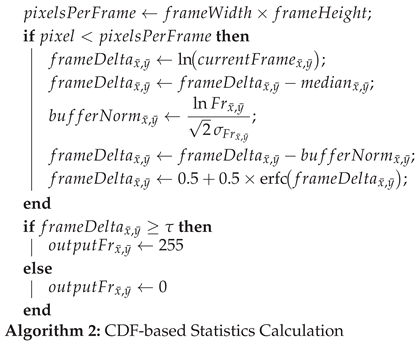 |
4. Results
In Figure 2, Figure 3, Figure 4 and Figure 5, we provide a series of images that our algorithm was tested on. In particular, we have experimented with different videos taken under varying illumination conditions with high-speed moving objects, such as a vehicle, as well as with humans in different scenarios. In the same set of figures, we juxtapose the output of our parallel lognormal algorithm with the state-of-the-art algorithms, namely MOG [3] and MOG2 [10] [11], and provide a qualitative analysis for comparison. For the implementation of MOG and MOG2 algorithms the deepgaze1, computer vision library has been utilized [44] using the Python programming language and OpenCV [45]. The video in Figure 2 is from [44] while videos in Figure 3 and Figure 4 are from [46]2. The implementation of our parallel algorithm can be found on Github3 while the output videos can be found on our YouTube channel (Background Subtraction playlist)4.
In all of the figures shown (Figure 2, Figure 3,Figure 4 and Figure 5), our training sample size has been kept at minimum, that is, 3 frames. In Figure 2 a moving vehicle is detected successfully across all video sequences. Furthermore, the qualitative analysis demonstrates that our parallel algorithm outperforms the state-of-the-art algorithms. The moving object, in this case, a vehicle is robustly segmented by our parallel algorithm. Although the MOG algorithm introduces some noise, the segmented vehicle appears with missing portions, particularly in the center. MOG2 achieves better segmentation of the vehicle, but significant noise is still present throughout the image. Figure 3 and Figure 4, feature substantial variations in lighting conditions. In spite of this, our algorithm outperforms MOG algorithm, while MOG2 is able to differentiate between foreground pixels and shadows (Figure 3). Finally, in Figure 4, our algorithm again outperforms both MOG and MOG2. In particular MOG algorithm performs poorly in low light conditions whereas MOG2 exhibits substantial noise, especially in areas containing stationary vehicles.
Finally, in Figure 5, a highway is shown with multiple vehicles moving at high speeds. The MOG algorithm struggles to effectively segment vehicles that are farther from the camera, though the segmentation improves when vehicles are closer, where more pixels represent the object. While the MOG2 algorithm performs well, it is still affected by noise. In contrast, our parallel algorithm successfully segments all vehicles, regardless of their distance from the camera, and exhibits significantly lower noise. In the upper part of the image, a flock of birds above the highway, visible in the original frame, is correctly segmented by all three algorithms.
The frame processing time has been estimated to be between 10 ms (100 fps) and 15 ms (67 fps) when using the NVIDIA GeForce GTX 970M while a processing time of 8 ms (125 fps) is achieved with the NVIDIA Titan X. As mentioned, the resolution used was and the buffer size was equal to 3 frames (). Finally, no post-processing has been implemented such as connected components or the flood-fill algorithm to improve the output of the background subtraction method.
In addition to the afore-mentioned resolution and buffer sizes, a number of experiments were carried out with higher -raw video- resolutions as well as different buffer sizes. The results are summarized in Table 3. It shows the average per–frame execution time and the corresponding throughput (fps) for four video sequences at three circular-buffer sizes (3, 8, and 10 frames). For the Full-HD sequences, that is, 1920 × 1080 (cars, cctv1, cctv5) processing time rises from roughly 20 ms to 24–28 ms as the buffer grows, translating to a drop from 50 fps to 36–42 fps. The 1280 × 720 highway sequence is consistently faster, sustaining up to 93 fps with a 3-frame buffer and about 70 fps with a 10-frame buffer. These results illustrate the classic accuracy–latency trade-off: larger temporal context improves model stability but reduces real-time throughput, especially for higher-resolution inputs.
In Figure 6, each row shows the same frame from a given dataset, whereas each column shows the result obtained with a different buffer size; specifically, columns 2–4 correspond to buffer sizes of 3, 8, and 10 frames, respectively. Increasing the buffer size reduces noise, but this comes at the cost of a lower frame rate, as reported in Table 3.
5. Conclusions and Future Work
In this research we have addressed the problem of background subtraction using a parallel algorithm implemented on GPU cores. Our proposed algorithm models pixel intensities using lognormal distributions. We compared our algorithm’s output with two of the most well-established Mixture of Gaussians (MOG) algorithms. The results obtained show that our method surpasses in most cases the state-of-the-art algorithms. Specifically, our algorithm combines the strengths of both MOG and MOG2, maintaining low noise levels similar to MOG while providing superior object segmentation akin to MOG2, but with significantly less noise. Furthermore, the throughput of our algorithm achieves a high number of processed frames, measured between 67 fps and 125 fps depending on the number of cores available in a given GPU, the video resolution as well as the buffer size. The parallel nature of the algorithm allows it to fully leverage additional cores, further increasing the frame rate. As demonstrated in the figures, the proposed algorithm quickly adapts to changes in lighting conditions and efficiently switches pixel states between background and foreground, thanks to the minimal sample size required to train the lognormal model.
Currently we are working on an enhancement that leverages KL-divergence, where we will compare distributions rather than individual pixels between the training and testing phases. For future research, we plan to adopt a Bayesian approach and optical flow [47,48,49] with the view to more accurately differentiate moving objects from static. Finally, we plan on testing our algorithm on a grid of GPUs to fully exploit the potential of our parallel algorithm. Our algorithm has numerous potential applications in transportation, surveillance, and other fields that involve detecting and tracking moving objects.
Supplementary Materials
The following supporting information can be downloaded at the website of this paper posted on Preprints.org.
Author Contributions
Conceptualization, S.D.; methodology, S.D.; software, E.R. and B.W; validation, E.R. and B.W.; investigation, S.D., E.R., and B.W.; writing—original draft preparation, S.D. and E.R.; supervision, S.D. and B.W. All authors have read and agreed to the published version of the manuscript.
Funding
This research received no external funding
Data Availability Statement
The source code for this research is available at: https://github.com/TSUrobotics/Parallel-Background-Subtraction. Demonstration videos generated for this research are available on the Robot Perception YouTube channel at: https://www.youtube.com/@robotperception6035.
Conflicts of Interest
The authors declare no conflicts of interest
| 1 | |
| 2 | |
| 3 | |
| 4 |
References
- Bardas, G.; Astaras, S.; Diamantas, S.; Pnevmatikakis, A. 3D tracking and classification system using a monocular camera. Wireless Personal Communications 2017, 92, 63–85.
- Diamantas, S.; Alexis, K. Optical Flow Based Background Subtraction with a Moving Camera: Application to Autonomous Driving. In Advances in Visual Computing. ISVC 2020. Lecture Notes in Computer Science; et al, G.B., Ed.; Springer Nature Switzerland, 2020.
- KaewTraKulPong, P.; Bowden, R. An Improved Adaptive Background Mixture Model for Real-time Tracking with Shadow Detection. In Video-Based Surveillance Systems; Springer US, 2002; chapter 11, pp. 135–144.
- Chen, M.; Yang, Q.; Li, Q.; Wang, G.; Yang, M.H. Spatiotemporal Background Subtraction Using Minimum Spanning Tree and Optical Flow. In Proceedings of the European Conference on Computer Vision (ECCV), 2014.
- NVIDIA. https://www.nvidia.com/en-gb/graphics-cards/, 2021.
- CUDA. https://developer.nvidia.com/cuda-toolkit, 2021.
- Diamantas, S.; Alexis, K. Modeling Pixel Intensities with Log-Normal Distributions for Background Subtraction. In Proceedings of the IEEE International Conference on Imaging Systems and Techniques, Beijing, China, 2017; pp. 1–6.
- Stauffer, C.; Grimson, W.E.L. Adaptive Background Mixture Models for Real-Time Tracking. In Proceedings of the 1999 Conference on Computer Vision and Pattern Recognition (CVPR ’99), 23-25 June 1999, Ft. Collins, CO, USA, 1999, pp. 2246–2252. [CrossRef]
- Xu, M.; Ellis, T. Illumination-invariant motion detection using colour mixture models. In Proceedings of the British Machine Vision Conference (BMVC 2001), 2001, pp. 163–172.
- Zivkovic, Z. Improved Adaptive Gaussian Mixture Model for Background Subtraction. In Proceedings of the 17th International Conference on Pattern Recognition, ICPR 2004, Cambridge, UK, August 23-26, 2004., 2004, pp. 28–31. [CrossRef]
- Zivkovic, Z.; van der Heijden, F. Efficient adaptive density estimation per image pixel for the task of background subtraction. Pattern Recognition Letters 2006, 27, 773–780.
- Elgammal, A.; Duraiswami, R.; Harwood, D.; Davis, L.S. Background and Foreground Modeling Using Nonparametric Kernel Density Estimation for Visual Surveillance. In Proceedings of the Proceeding of the IEEE, November 2002, Vol. 90, pp. 1151–1163.
- Heikkilä, M.; Pietikäinen, M. A Texture-Based Method for Modeling the Background and Detecting Moving Objects. IEEE Transactions on Pattern Analysis and Machine Intelligence 2006, 28, 657–662. [CrossRef]
- Lee, J.; Park, M. An Adaptive Background Subtraction Method Based on Kernel Density Estimation. Sensors 2012, 12, 12279–12300.
- Barnich, O.; Droogenbroeck, M.V. ViBe: A Universal Background Subtraction Algorithm for Video Sequences. IEEE Transactions on Image Processing 2011, 20, 1709–1724. [CrossRef]
- Shen, Y.; Hu, W.; Liu, J.; Yang, M.; Wei, B.; Chou, C.T. Efficient background subtraction for real-time tracking in embedded camera networks. In Proceedings of the Proceedings of the 10th ACM Conference on Embedded Network Sensor Systems, 2012, pp. 295–308.
- Tabkhi, H.; Bushey, R.; Schirner, G. Algorithm and architecture co-design of Mixture of Gaussian (MoG) background subtraction for embedded vision. In Proceedings of the Proceedings of Asilomar Conference on Signals, Systems and Computers, Pacific Grove, CA, USA, 2013.
- Godbehere, A.B.; Matsukawa, A.; Goldberg, K.Y. Visual tracking of human visitors under variable-lighting conditions for a responsive audio art installation. In Proceedings of the American Control Conference, ACC 2012, Montreal, QC, Canada, June 27-29, 2012, 2012, pp. 4305–4312.
- Yao, J.; Odobez, J.M. Multi-Layer Background Subtraction Based on Color and Texture. In Proceedings of the 2007 IEEE Computer Society Conference on Computer Vision and Pattern Recognition (CVPR 2007), 18-23 June 2007, Minneapolis, Minnesota, USA, 2007. [CrossRef]
- Zhang, C.; Tabkhi, H.; Schirner, G. A GPU-Based Algorithm-Specific Optimization for High-Performance Background Subtraction. In Proceedings of the 2014 43rd International Conference on Parallel Processing, 2014, pp. 182–191. [CrossRef]
- Szwoch, G.; Ellwart, D.; Czyżewski, A. Parallel implementation of background subtraction algorithms for real-time video processing on a supercomputer platform. Journal of Real-Time Image Processing 2016, 11, 111–125.
- Braham, M.; Droogenbroeck, M.V. Deep Background Subtraction with Scene-Specific Convolutional Neural Networks. In Proceedings of the The 23rd International Conference on Systems, Signals and Image Processing, 2016.
- Rai, N.K.; Chourasia, S.; Sethi, A. An Efficient Neural Network Based Background Subtraction Method. In Advances in Intelligent Systems and Computing; Bansal, J.; Singh, P.; Deep, K.; Nagar, M.P.A., Eds.; Springer, 2013; pp. 453–460.
- Radke, R.J.; Andra, S.; Al-Kofahi, O.; Roysam, B. Image Change Detection Algorithms: A Systematic Survey. IEEE Transactions on Image Processing 2005, 14, 294–307. [CrossRef]
- Candès, E.J.; Li, X.; Ma, Y.; Wright, J. Robust Principal Component Analysis? Journal of the ACM 2011, 58, 11:1–11:37. [CrossRef]
- Bouwmans, T.; Sobral, A.; Javed, S.; Jung, S.K.; Zahzah, E. Decomposition into Low-Rank plus Additive Matrices for Background/Foreground Separation: A Review for a comparative evaluation with a large-scale dataset. Computer Science Review 2017, 23, 1–71. [CrossRef]
- Yong, H.; Meng, D.; Zuo, W.; Zhang, L. Robust Online Matrix Factorization for Dynamic Background Subtraction. IEEE Transactions on Pattern Analysis and Machine Intelligence 2018, 40, 1726–1740. [CrossRef]
- Giraldo, J.H.; Bouwmans, T. GraphBGS: Background Subtraction via Recovery of Graph Signals. In Proceedings of the 2020 25th International Conference on Pattern Recognition (ICPR), 2021, pp. 6881–6888. [CrossRef]
- Hofmann, M.; Tiefenbacher, P.; Rigoll, G. Background Segmentation with Feedback: The Pixel-Based Adaptive Segmenter. In Proceedings of the 2012 IEEE Computer Society Conference on Computer Vision and Pattern Recognition Workshops, 2012, pp. 38–43. [CrossRef]
- Sobral, A.; Vacavant, A. A Comprehensive Review of Background Subtraction Algorithms Evaluated with Synthetic and Real Videos. Computer Vision and Image Understanding 2014, 122, 4–21. [CrossRef]
- Wang, Y.; Jodoin, P.M.; Porikli, F.; Konrad, J.; Benezeth, Y.; Ishwar, P. CDnet 2014: An Expanded Change Detection Benchmark Dataset. In Proceedings of the Proc. IEEE CVPR Workshops, 2014, pp. 393–400.
- Bouwmans, T.; Javed, S.; Sultana, M.; Jung, S.K. Deep Neural Network Concepts for Background Subtraction: A Systematic Review and Comparative Evaluation. Neural Networks 2019, 117, 8–66. [CrossRef]
- Braham, M.; Van Droogenbroeck, M. Deep Background Subtraction with Scene-Specific Convolutional Neural Networks. In Proceedings of the Proc. Intl. Conf. on Systems, Signals and Image Processing (IWSSIP), 2016, pp. 1–4. [CrossRef]
- Babaee, M.; Dinh, D.T.; Rigoll, G. A Deep Convolutional Neural Network for Video Sequence Background Subtraction. Pattern Recognition 2018, 76, 635–649. [CrossRef]
- Lim, L.A.; Keleş, H.Y. Learning Multi-Scale Features for Foreground Segmentation. Pattern Analysis and Applications 2020, 23, 1369–1380. [CrossRef]
- Cioppa, A.; Van Droogenbroeck, M.; Braham, M. Real-Time Semantic Background Subtraction. In Proceedings of the Proc. IEEE Intl. Conf. on Image Processing (ICIP), 2020, pp. 3214–3218. [CrossRef]
- Tezcan, M.O.; Ishwar, P.; Konrad, J. BSUV-Net: A Fully-Convolutional Neural Network for Background Subtraction of Unseen Videos. In Proceedings of the 2020 IEEE Winter Conference on Applications of Computer Vision (WACV), 2020, pp. 2763–2772. [CrossRef]
- Zhang, C.; Tabkhi, H.; Schirner, G. A GPU-Based Algorithm-Specific Optimization for High-Performance Background Subtraction. In Proceedings of the Proc. Intl. Conf. on Parallel Processing (ICPP), 2014, pp. 182–191. [CrossRef]
- Karagöz, M.F.; Aktas, M.; Akgün, T. CUDA implementation of ViBe background subtraction algorithm on jetson TX1/TX2 modules. In Proceedings of the 2018 26th Signal Processing and Communications Applications Conference (SIU), 2018, pp. 1–4. [CrossRef]
- Kryjak, T.; Gorgon, M. Real-Time Implementation of Background Modelling Algorithms in FPGA Devices. In New Trends in Image Analysis and Processing – ICIAP 2015 Workshops; Springer, 2015; Vol. 9281, Lecture Notes in Computer Science, pp. 519–526. [CrossRef]
- Sehairi, K.; Chouireb, F. Implementation of Motion Detection Methods on Embedded Systems: A Performance Comparison. International Journal of Technology 2023, 14, 510–521. [CrossRef]
- Sun, Z.; Zhu, L.; Qin, S.; Yu, Y.; Ju, R.; Li, Q. Road Surface Defect Detection Algorithm Based on YOLOv8. Electronics 2024, 13, 2413. [CrossRef]
- Wang, J.; Meng, R.; Huang, Y.; Zhou, L.; Huo, L.; Qiao, Z.; Niu, C. Road Defect Detection Based on Improved YOLOv8s Model. Scientific Reports 2024, 14, 16758. [CrossRef]
- Deebgaze Computer Vision library. https://github.com/mpatacchiola/deepgaze, 2017.
- OpenCV. http://opencv.willowgarage.com/wiki/, 2017.
- MARE’s Computer Vision Study. http://study.marearts.com/, 2017.
- Diamantas, S. Biological and Metric Maps Applied to Robot Homing. PhD thesis, School of Electronics and Computer Science, University of Southampton, 2010.
- Diamantas, S.C.; Oikonomidis, A.; Crowder, R.M. Towards Optical Flow-Based Robotic Homing. In Proceedings of the Proceedings of the International Joint Conference on Neural Networks (IEEE World Congress on Computational Intelligence), Barcelona, Spain, 2010.
- Diamantas, S.C.; Oikonomidis, A.; Crowder, R.M. Depth Computation Using Optical Flow and Least Squares. In Proceedings of the IEEE/SICE International Symposium on System Integration, Sendai, Japan, 2010; pp. 7–12.
Figure 1.
Lognormal distributions obtained for every pixel during the training phase by sampling temporal pixel values over a three-frame buffer. The buffer is constantly updated with newer frames by evicting the old ones.
Figure 1.
Lognormal distributions obtained for every pixel during the training phase by sampling temporal pixel values over a three-frame buffer. The buffer is constantly updated with newer frames by evicting the old ones.

Figure 2.
Top to bottom (car dataset): Raw image; MOG algorithm; MOG2 algorithm; Parallel Lognormal (proposed algorithm).
Figure 2.
Top to bottom (car dataset): Raw image; MOG algorithm; MOG2 algorithm; Parallel Lognormal (proposed algorithm).
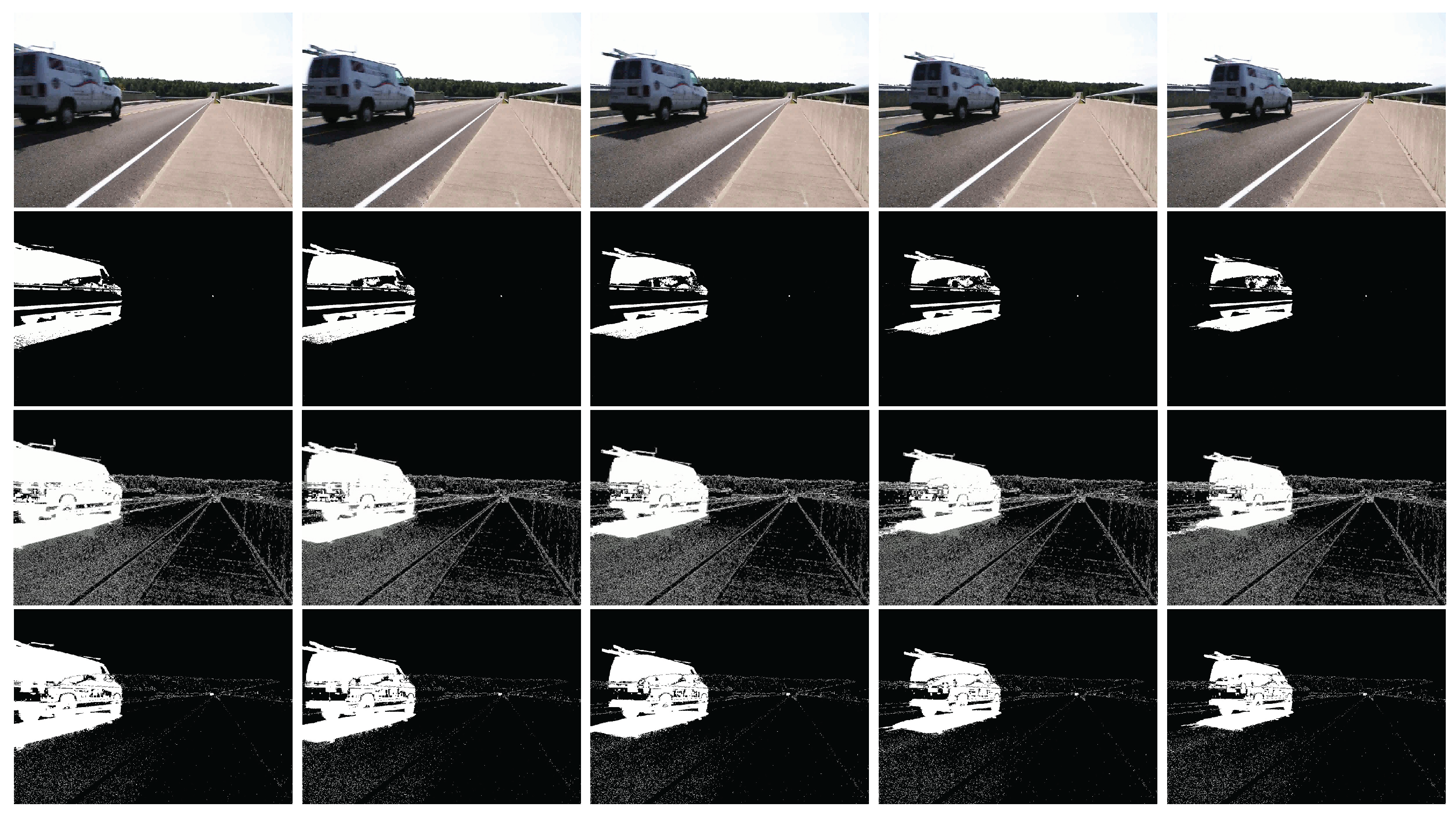
Figure 3.
Top to bottom (cctv1 dataset): Raw image; MOG algorithm; MOG2 algorithm; Parallel Lognormal (proposed algorithm).
Figure 3.
Top to bottom (cctv1 dataset): Raw image; MOG algorithm; MOG2 algorithm; Parallel Lognormal (proposed algorithm).
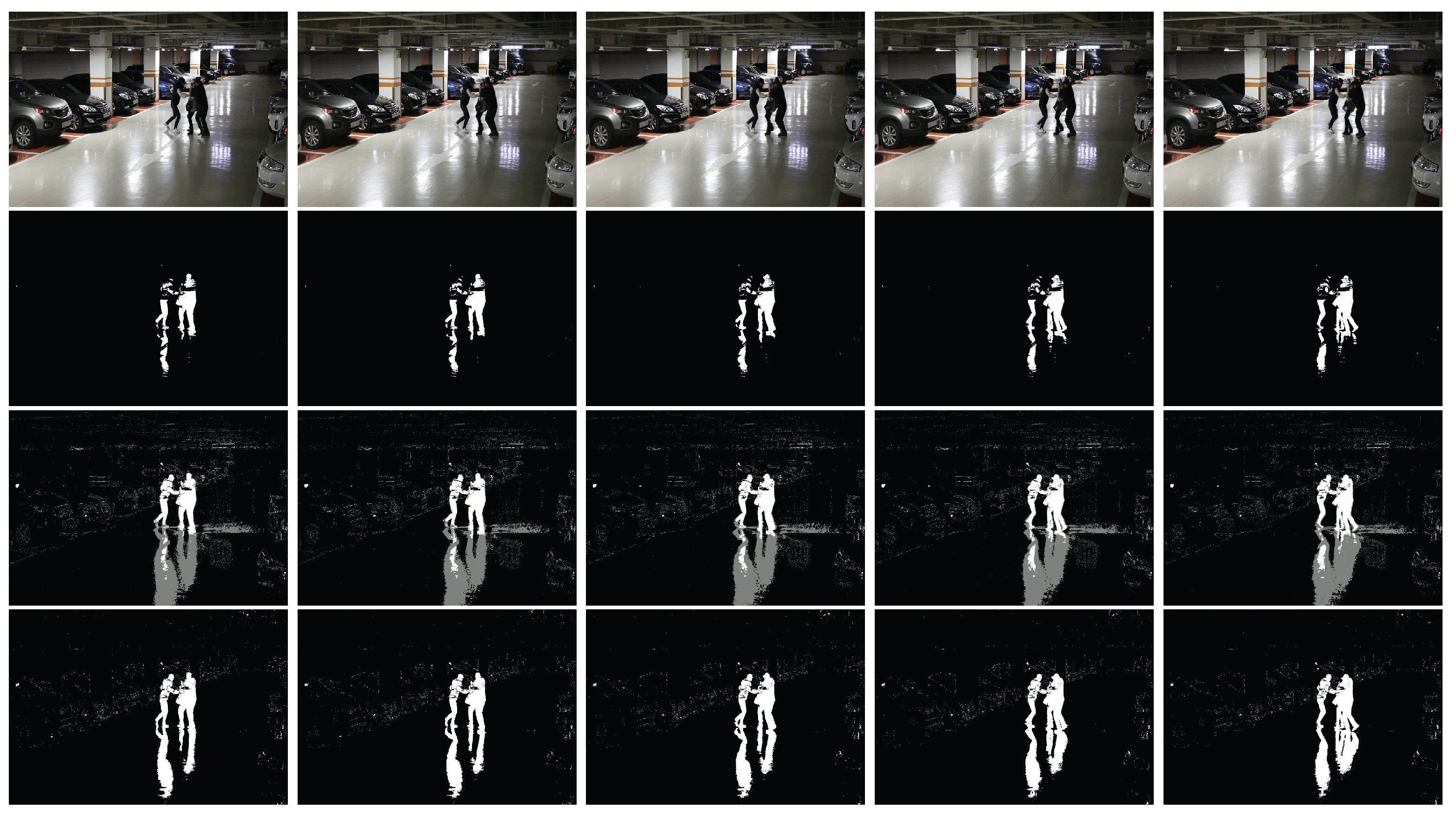
Figure 4.
Top to bottom (cctv5 dataset): Raw image; MOG algorithm; MOG2 algorithm; Parallel Lognormal (proposed algorithm).
Figure 4.
Top to bottom (cctv5 dataset): Raw image; MOG algorithm; MOG2 algorithm; Parallel Lognormal (proposed algorithm).
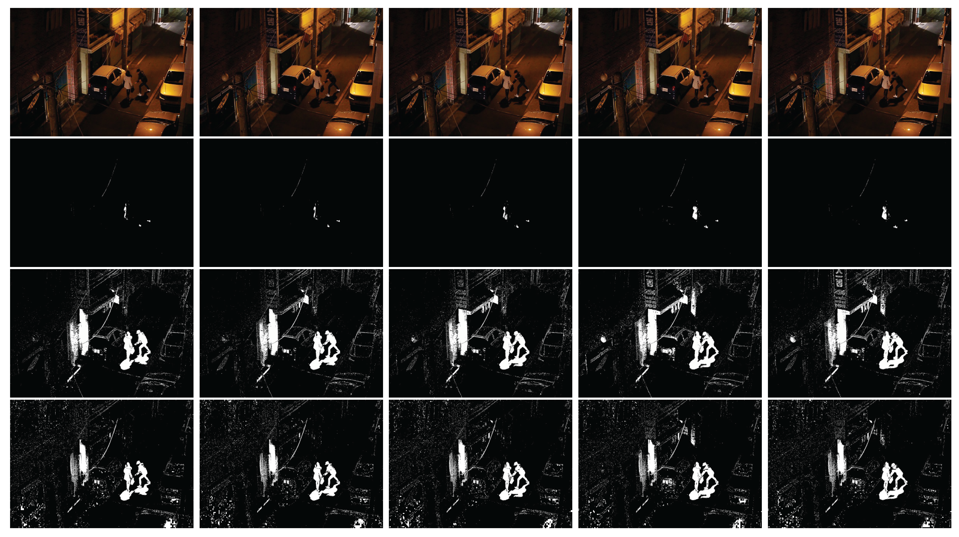
Figure 5.
Top to bottom (highway dataset): Raw image; MOG algorithm; MOG2 algorithm; Parallel Lognormal (proposed algorithm).
Figure 5.
Top to bottom (highway dataset): Raw image; MOG algorithm; MOG2 algorithm; Parallel Lognormal (proposed algorithm).
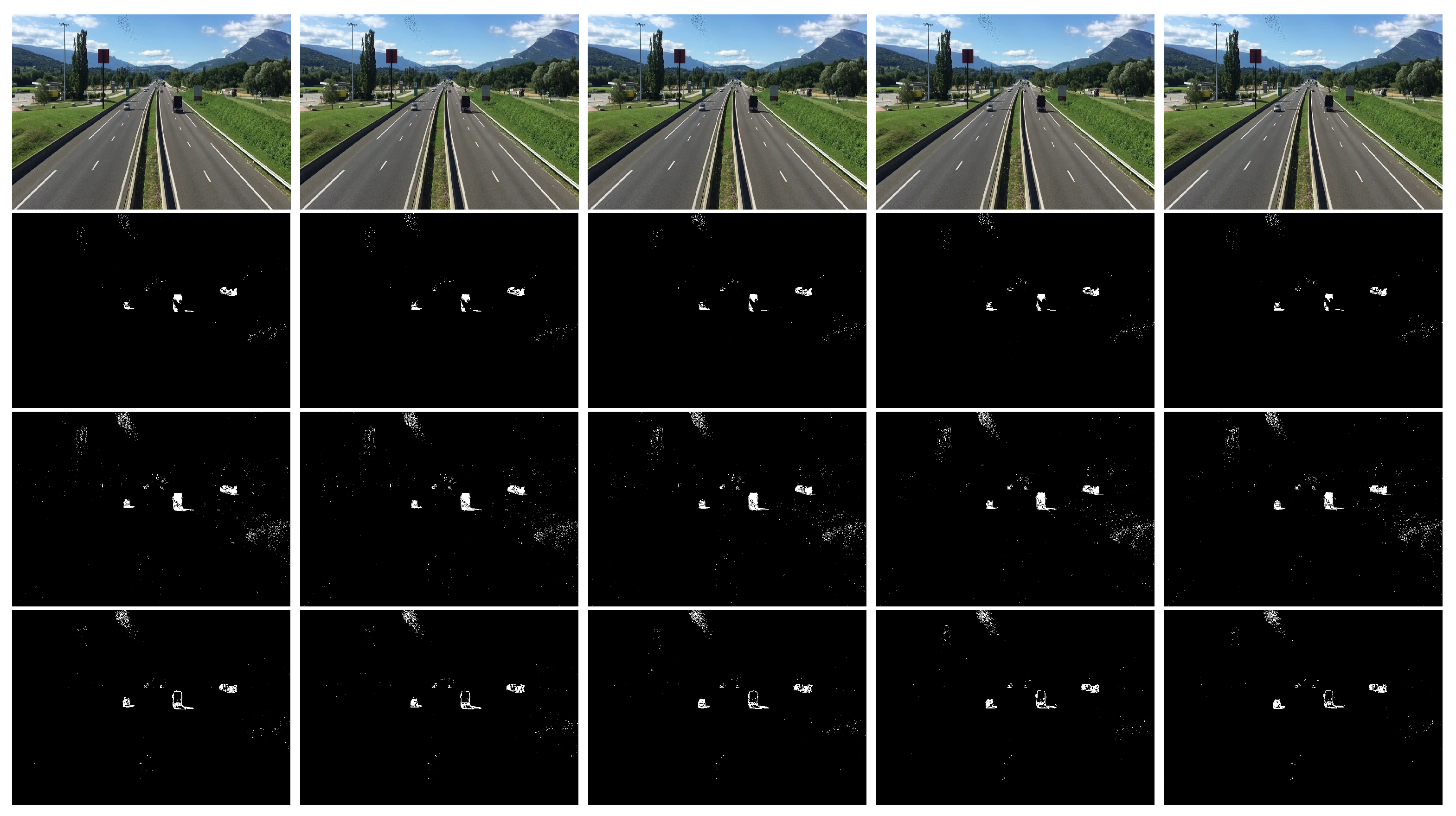
Figure 6.
Rows top-bottom: car, cctv1, cctv5 datasets. Columns left-right: raw images; buffer size = 3; buffer size = 8; buffer size = 10.
Figure 6.
Rows top-bottom: car, cctv1, cctv5 datasets. Columns left-right: raw images; buffer size = 3; buffer size = 8; buffer size = 10.
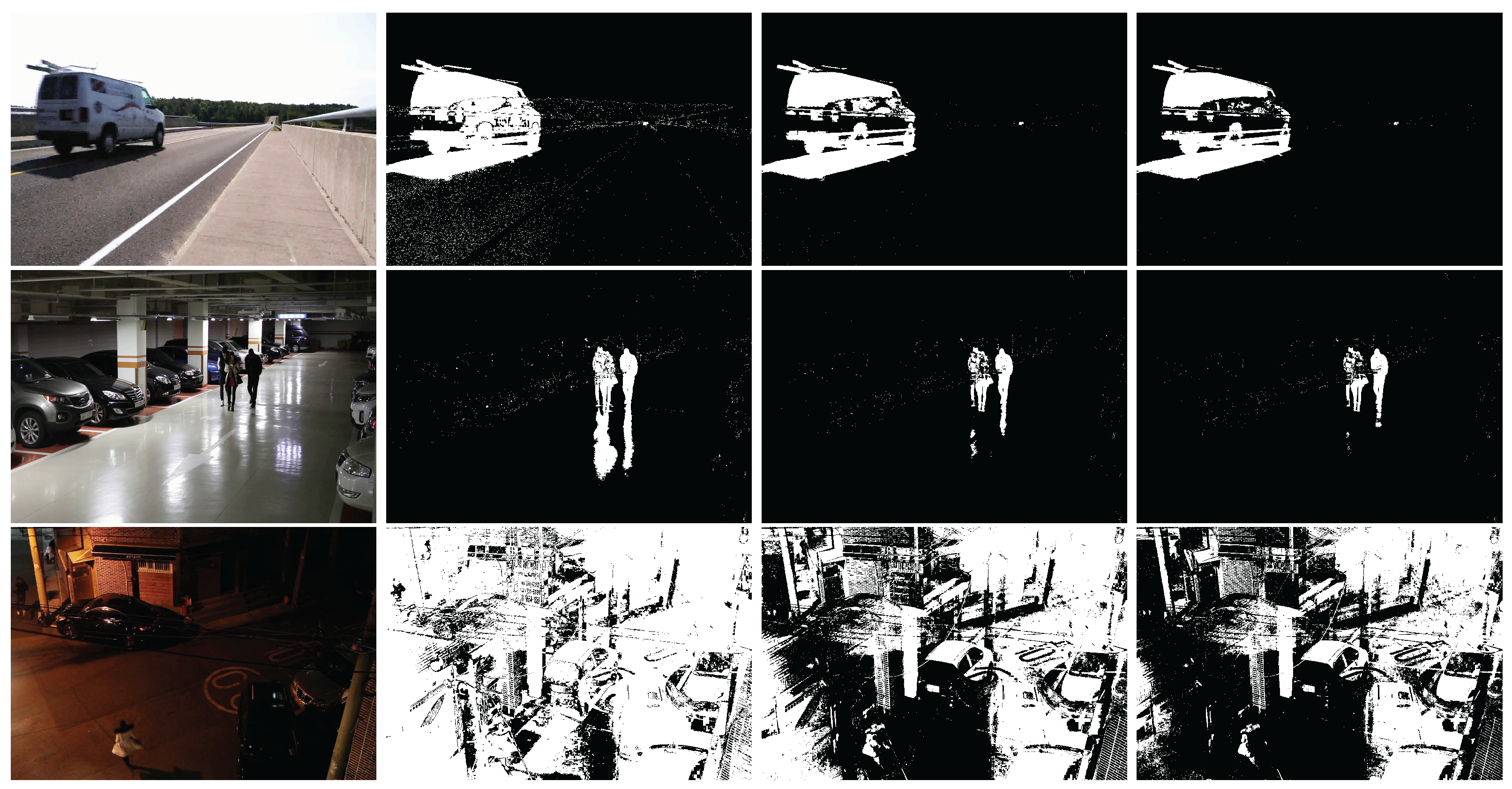

Table 1.
Description of Variables in Algorithm 1
| Variable | Description |
|---|---|
| Total number of pixels per frame, | |
| calculated as frame width × frame height. | |
| Current pixel index. | |
| Total number of frames in the buffer. | |
| Sum of all pixel intensities | |
| across frames for given coordinates . | |
| Mean pixel intensity at over all frames. | |
| Log-normal Buffer | |
| Sum of all pixel intensities across . | |
| Median of | |
| Standard deviation of . |
Table 2.
Description of Variables in Algorithm 2
| Variable | Description |
|---|---|
| Total number of pixels per frame, | |
| calculated as frame width × frame height. | |
| latest frame to be processed. | |
| log-normalized buffer frame | |
| (i.e. equation 5) | |
| input variability amount | |
| background subtracted image |
Table 3.
Average per–frame processing time (ms) and resulting frame-rate (fps) for three circular-buffer sizes. A larger buffer allows richer temporal context but increases processing latency. All videos are at their native resolution.
Table 3.
Average per–frame processing time (ms) and resulting frame-rate (fps) for three circular-buffer sizes. A larger buffer allows richer temporal context but increases processing latency. All videos are at their native resolution.
| Dataset (resolution) | 3-frame buffer | 8-frame buffer | 10-frame buffer | |||
|---|---|---|---|---|---|---|
| Time [ms] | fps | Time [ms] | fps | Time [ms] | fps | |
| cars (1920 × 1080) | 19.61 | 51.0 | 23.64 | 42.3 | 23.96 | 41.7 |
| cctv1 (1920 × 1080) | 19.85 | 50.4 | 23.89 | 41.9 | 24.26 | 41.2 |
| cctv5 (1920 × 1080) | 20.26 | 49.4 | 25.82 | 38.7 | 27.69 | 36.1 |
| highway (1280 × 720) | 10.80 | 92.6 | 13.63 | 73.3 | 14.20 | 70.4 |
| Buffer size = number of previous frames kept in memory for temporal reasoning. | ||||||
Disclaimer/Publisher’s Note: The statements, opinions and data contained in all publications are solely those of the individual author(s) and contributor(s) and not of MDPI and/or the editor(s). MDPI and/or the editor(s) disclaim responsibility for any injury to people or property resulting from any ideas, methods, instructions or products referred to in the content. |
© 2025 by the authors. Licensee MDPI, Basel, Switzerland. This article is an open access article distributed under the terms and conditions of the Creative Commons Attribution (CC BY) license (http://creativecommons.org/licenses/by/4.0/).
Copyright: This open access article is published under a Creative Commons CC BY 4.0 license, which permit the free download, distribution, and reuse, provided that the author and preprint are cited in any reuse.


