Submitted:
03 June 2025
Posted:
04 June 2025
You are already at the latest version
Abstract
We investigate whether the hot-hand belief, typically viewed as a cognitive illusion, endogenously influences portfolio choices in a financial experiment. Participants allocated funds across assets with randomly generated prices, under conditions of known probabilities and varying levels of risk. In a two-stage setup, participants were exposed to random price sequences in the initial stage both to learn about the game and to induce a perception of successful performance streaks. Then, they encountered additional random price paths in the second stage. Our findings show that the hot-hand belief, measured by increased purchases following gains, was effectively induced but did not persist throughout the experiment. Instead, loss aversion prevailed when participants faced sustained negative trends. The study highlights the dynamic interaction between cognitive heuristics and emotional biases, suggesting that belief in trend continuation is shaped by performance feedback but ultimately constrained by the reluctance to realize losses.
Keywords:
hot-hand belief
; loss aversion
; portfolio choice
; belief formation
1. Introduction
This paper investigates whether the hot-hand belief, typically viewed as a cognitive illusion, can endogenously influence individual portfolio choices in a financial context. Unlike previous studies that consider the belief as exogenous and assigned by third parties, such as investors reacting to mutual fund performance [1,2] or participants following simulated experts [3], we examine whether individuals develop this belief from their own investment experience. Specifically, we test whether perceived personal success in asset selection affects subsequent behavior, even when asset prices follow a purely random path.
To explore this question, we conducted a controlled laboratory experiment using a hypothetical financial market. Participants allocated resources among four assets with different risk-return profiles, all with prices generated randomly according to known probabilities. The experiment followed a two-stage design. In the first stage, participants encountered random price sequences to become familiar with the game and to develop a perception of being on successful performance streaks. Subsequently, they faced additional random price paths in the second stage.
Our approach offers a distinct contribution to the literature. By inducing the hot-hand belief through personal experience and observing its behavioral consequences under controlled conditions, we provide clean evidence on the formation and decay of this belief. The design avoids confounding influences present in studies where beliefs are externally attributed, and it highlights how minor differences in early outcomes can alter perceptions and behavior, even in environments governed by randomness.
We define the hot-hand belief as an incorrect expectation about price formation, measured by an increased likelihood of repurchasing assets after gains or upward price movements. In contrast, loss aversion refers to the tendency to retain losing assets and prematurely sell winners. While successful performance triggered hot-hand behavior, the effect diminished over time. When participants faced consistent negative price trends, loss aversion dominated, reducing the influence of prior success and reshaping portfolio decisions.
This study contributes to the behavioral finance literature by demonstrating that the hot-hand belief can be endogenously generated through feedback-driven learning and by tracking how it evolves across different investment conditions. Crucially, our results show that the influence of the hot-hand belief is not isolated but interacts with loss aversion, a robust feature of investor behavior. When sustained losses occurred, the tendency to avoid realizing them gradually overpowered the optimistic bias driven by past success. Together, these findings offer new insights into how cognitive heuristics and emotional biases jointly shape decision-making under risk, and they highlight important limitations in models based solely on rational expectations.
2. Literature Review and Theoretical Background
Expected Utility Theory (EU) is the traditional framework for modeling investor behavior under risk. It assumes that rational agents choose among risky alternatives to maximize the expected value of a utility function, subject to axioms such as completeness, transitivity, continuity, and independence [4,5,6,7]. Despite its theoretical elegance and normative appeal, EU has limited empirical support. Systematic violations of its axioms have been observed, especially when individuals exhibit inconsistent attitudes toward risk. For example, preferences often reverse depending on whether outcomes are framed as gains or losses, and individuals frequently display risk aversion for gains and risk-seeking for losses, contrary to EU predictions [8,9,10].
To address these violations, Kahneman and Tversky [11] developed Prospect Theory (PT), which has become a cornerstone of behavioral economics. PT models decision-making under risk based on changes in wealth relative to a reference point rather than final outcomes. It introduces a value function that is concave for gains and convex for losses, and steeper for losses than for gains, capturing the phenomenon known as loss aversion—meaning that losses loom larger than equivalent gains. In addition, PT proposes a probability weighting function, in which small probabilities tend to be overweighted and large probabilities underweighted, further departing from the linear treatment of probabilities in EU. These features allow PT to explain several empirical anomalies, including the certainty effect, isolation effect, and framing effects [12,13,14].
Loss aversion plays a central role in explaining behavioral anomalies such as the disposition effect, which refers to the tendency of investors to sell winning assets too early and hold on to losing ones for too long [15,16]. In the context of PT, this pattern arises because individuals evaluate outcomes relative to a reference point, often the purchase price, and become risk-averse when facing gains and risk-seeking when facing losses. A gain relative to the reference point feels satisfactory and motivates realization, while a loss feels painful and leads the investor to hold the asset in the hope of recovery. As a result, decisions are not based solely on expected utility or updated probabilities but are influenced by emotional responses to perceived gains and losses.
Empirical evidence for the disposition effect has been documented both in real trading environments and in laboratory experiments [17,18]. The literature suggests that this bias is robust across contexts and is associated with suboptimal portfolio performance, particularly in volatile markets. While PT provides a theoretical explanation for the disposition effect, it does not preclude the coexistence of other belief-driven behaviors that influence investment decisions. One such belief, which may interact or even conflict with loss aversion, is the hot-hand belief: the expectation that recent success is likely to continue, even in the absence of objective autocorrelation. Understanding how these behavioral forces operate together is essential to capture the complexity of investor behavior in dynamic financial environments.
Originally studied in the context of sports, the hot-hand belief is commonly interpreted as a cognitive illusion, resulting from representativeness heuristics, whereby people expect short random sequences to resemble the long-run properties of the process that generated them [19,20]. In this view, individuals tend to overinfer from small samples, treating recent outcomes as informative signals of ability or trend, even in purely random environments. As a result, they may form expectations of continued success based solely on prior streaks, regardless of the objective statistical structure of the situation.
This cognitive bias leads individuals to perceive patterns or momentum where none exists, particularly when the underlying process is governed by independent random draws. In this view, the hot-hand belief is closely related to the misperception of randomness, and it emerges from a broader tendency to overinfer from small samples [19], anchoring judgments on recent outcomes and exhibiting overconfidence in perceived personal performance [21]. These mechanisms are well documented in cognitive psychology and form the foundation for understanding how beliefs like the hot-hand can arise even in environments characterized by objective unpredictability. Importantly, they help explain why such beliefs persist despite contradictory evidence, especially when individuals receive performance feedback that appears to confirm their expectations.
The most influential empirical investigation of the hot-hand belief was conducted by Gilovich, Vallone, and Tversky [22]. Using player statistics from professional basketball games and survey responses from fans and coaches, the authors tested whether success in prior shots increased the likelihood of subsequent success. Despite widespread belief among participants that players could become “hot,” their analysis found no evidence of actual positive autocorrelation in shooting performance. They concluded that the hot-hand was a cognitive illusion, a product of misperceiving random sequences, and introduced the concept of the “hot-hand fallacy” to describe this mismatch between belief and reality. Their findings became a cornerstone in the literature on judgment under uncertainty and were widely cited as evidence of systematic errors in human reasoning about chance.
More than three decades after the original study, Miller and Sanjurjo [23] revisited the statistical methodology used by Gilovich, Vallone, and Tversky and demonstrated that their conclusions were affected by a subtle but systematic bias. The original analysis underestimated the likelihood of success following streaks due to a selection bias that arises when computing conditional probabilities in finite sequences. Specifically, they showed that in a sequence of random outcomes, the empirical probability of success following previous successes is expected to be lower than the true probability, even when outcomes are independent. After correcting for this bias, Miller and Sanjurjo found statistically significant evidence of a hot-hand effect in the same basketball data previously analyzed. Their findings reignited the debate and prompted a broader reexamination of how the hot-hand belief is measured and interpreted in empirical studies.
In the field of finance, the hot-hand belief has also been studied as a factor influencing investor behavior, particularly in contexts where individuals evaluate the recent performance of third parties such as fund managers or financial “experts.” Several studies have documented that investors tend to allocate more resources to mutual funds that have performed well in the recent past, a behavior interpreted as evidence of hot-hand belief [1,2]. In these cases, the belief is modeled as exogenous to the decision-maker. That is, the investor does not believe in their own streakiness, but rather attributes skill or predictive power to the recent success of others. This framework is conceptually similar to the hot-hand belief in sports, where spectators believe that a player who has made several successful shots is more likely to continue performing well. Experimental studies such as Huber et al. [3] further support this interpretation by showing that participants favor options associated with recent success, even when outcomes are generated by randomized processes.
While prior research has typically treated the hot-hand belief as an exogenous perception about others, our study investigates whether this belief can emerge endogenously from the investor’s own experience. Instead of observing the past performance of external agents, participants in our experiment make repeated portfolio decisions and receive direct feedback on their outcomes. This setup allows us to test whether personal streaks of success lead individuals to expect continued favorable results, even when asset prices follow a purely random process. This approach provides a unique opportunity to isolate the formation of the belief and observe its persistence or attenuation over time, particularly in interaction with other behavioral forces such as loss aversion.
3. Experimental Design
3.1. Design Overview
The experimental task was implemented using the z-Tree software package [24], version 3.6.7. The experiment consisted of two stages, during which participants made repeated investment decisions in a simulated financial market. In each round, they could allocate resources among four types of assets: one high-risk (Asset A), one medium-risk (Asset B), one low-risk (Asset C), and one risk-free asset (cash). The first stage served as a familiarization phase, in which participants learned the structure of the task, observed how asset prices evolved, and made six investment decisions without monetary consequences. In the second stage, participants made ten additional investment decisions, this time with a chance to earn a monetary reward based on their final portfolio value.
At each decision round, participants could buy any quantity of the available assets at the current displayed prices. All purchases were automatically liquidated at the beginning of the next round, with prices updated according to a predefined random process. Assets could be repurchased in subsequent rounds, with no transaction costs or inflation adjustments. The price-generation mechanism, which guaranteed random but differentiated dynamics across assets, is detailed in the next subsection.
At the beginning of each investment round, participants received an endowment of R$ 5,000, which could be allocated among the available assets or held in cash. The cash option functioned as a risk-free asset and did not accrue interest. Participants were not allowed to borrow or take short positions. If, at any point, the total value of a participant’s portfolio reached zero, the session was automatically terminated for that individual. For reference, the nominal value of R$ 5,000 corresponded to approximately US$ 1,199, using the exchange rate of 4.17 Reais per US dollar on November 12, 2019 [25].
After each investment decision, participants were shown the updated value of their portfolios in the following round, allowing them to track their performance over time. During the first stage, they also received feedback comparing their current outcome to their average performance across previous rounds. A message reading “You have outperformed your average game performance” was displayed when the result was above average, while “You underperformed your average game performance” appeared when it was below. This mechanism was designed to reinforce perceptions of success or failure, contributing to the formation of performance-based expectations.
At the beginning of each session, participants received standardized instructions explaining the rules of the experiment, including the mechanics of decision-making and the functioning of the price system. The instructor followed a predefined script to ensure consistency across sessions. Participants were also shown how to interact with the interface: how to view asset prices, enter decisions, and execute purchases on the game screen.
Participants were informed about the price formation process in simplified terms. They were told that all assets started at the same initial price and that future price changes would occur randomly. Prices could either increase or decrease at each round, with equal probability, and the size of the variation differed across assets according to their risk classification: high, medium, or low. The underlying structure followed a two-step random draw, detailed in the next subsection.
Asset prices were generated by a fixed algorithm that remained constant throughout the experiment. All assets began at R$ 100 in the first round. In each subsequent period, prices were updated through a two-step random process. First, the direction of the price change (increase or decrease) was determined independently for each asset, with equal probability (). Second, the magnitude of the change was randomly selected from three equally likely values, specific to each asset: R$ 21, 23, or 25 for asset A (high risk); R$ 11, 13, or 15 for B (medium risk); and R$ 1, 3, or 5 for C (low risk). Both the direction and magnitude of the price variation were drawn independently. The resulting distributions are summarized in Table 1.
The price distributions were chosen to serve two primary purposes. First, they ensured that belief in price autocorrelation would reflect a cognitive bias, since all assets had an equal probability of increasing or decreasing. This neutrality implies that any perception of trend persistence, which is central to the hot-hand belief, would not stem from the price-generating process itself but from the participant’s interpretation of observed outcomes. Second, the use of three distinct values for price variation in each asset enabled participants to infer trends without requiring advanced analytical skills. This feature was intended to reduce the familiarity bias, which arises when individuals feel overly confident in evaluating simple or repetitive lotteries [26,27,28]. As in coin-tossing tasks, investors may perceive patterns even in environments where the probabilities are symmetric [29]. By using a random walk structure with multiple variation levels, we created a setting that was simultaneously unpredictable and suggestive of structure. This strategy enhanced the design proposed by Huber et al. [3], replacing abstract betting choices with portfolio decisions involving assets with differentiated volatility.
An additional advantage of our design is that the resulting distributions of multi-asset portfolio returns were approximately normal. This property allowed us to describe asset performance using only mean and variance, avoiding analytical complications associated with non-quadratic utility functions. The use of normally distributed returns aligns with previous experimental designs in finance, such as in Weber and Camerer [30].
Our experimental design also addressed ambiguity bias while maintaining control over familiarity. Ambiguity, as first discussed by Ellsberg [8], refers to the uncertainty individuals experience when faced with complex or ill-defined probability distributions. In contrast to earlier studies such as Weber and Camerer [16], which included seven purchase options, we limited our experiment to three risky assets and one risk-free alternative. Each risky asset was associated with a clearly defined risk and return profile: high, medium, or low. This structure allowed participants to form expectations within a well-specified decision environment and reduced ambiguity in portfolio selection.
Balancing familiarity and ambiguity in the multi-asset portfolio was essential to defining the relevant information set for belief formation. Following the approach suggested by Ayton and Fischer [29], our design enabled participants to form hot-hand beliefs based on observed price dynamics, rather than explicit cues or instructions. Participants made investment decisions by interpreting graphical displays of past asset prices, and could refer to indicators such as recent averages, historical maxima, and minima. These elements were presented directly on the game screen and served as visual anchors for individual expectations about future performance.
The experiment was structured as a two-stage game with automatic liquidation of assets between rounds. This feature, inspired by previous studies [16,30,31,32,33], required participants to make active portfolio decisions at every round, including the deliberate repurchase of any asset they wished to retain. The two-stage structure also allowed us to separate the initial phase of performance feedback and familiarization from the phase in which participants’ decisions had financial consequences.
The price series generated by our algorithm followed the expected behavior and exhibited approximately normal distributions. All assets passed the Shapiro-Wilk normality test, with p-values greater than 0.05, indicating no significant deviation from normality. Figure 1 displays the time series generated by our simulation procedures. Asset A is represented by a solid line with circular markers, Asset B by a dotted line with square markers, and Asset C by a dash-dotted line with cross markers.
3.2. Procedure and Treatments
The experiment received approval from two Research Ethics Committees: decision No. 2.558.540 at the University of Brasília (UnB) and decision No. 2.850.741 at the Federal University of Tocantins (UFT). Before final implementation, we conducted pilot sessions to evaluate the clarity of on-screen instructions, the participants’ understanding of the task, and other design components. One of the goals was to assess whether participants would behave differently depending on their awareness of the price-generating process, as suggested by Barberis and Thaler [34].
The pilot sessions involved two groups of 14 undergraduate students from UFT. One group was explicitly informed about the risk structure of each asset, while the other was only told that prices were randomly determined. In the informed group, the instructor explained that asset A had high risk, asset B had medium risk, and asset C had low risk, with both gains and losses reflecting these levels. Participants in this group exhibited a significant difference in their purchasing behavior following price increases versus decreases, which aligned more closely with the behavioral patterns under investigation. Based on these results, we adopted the known-distribution format described by Weber and Camerer [16] in the final experiment. The pilot sessions also contributed to refining the game instructions, validating the information displayed on screen, and determining the optimal number of rounds.
A total of 226 undergraduate students from various academic programs at UFT and UnB were recruited for the experiment. After applying exclusion criteria, the final sample consisted of 208 participants. Eighteen individuals were removed due to a misunderstanding of the game mechanics, specifically the incorrect belief that they could only purchase one asset or a single unit per round. The full dataset from the valid sample is publicly available through Mendeley Data [35].
The experimental sessions were conducted between August 2018 and May 2019 in computer laboratories at both universities. Each session included no more than 20 participants, seated at spaced-out workstations to prevent communication. All participants signed a written informed consent form prior to the activity. Each session lasted approximately 30 minutes. The lowest and highest payments made to participants were R$ 9.50 and R$ 11.00, respectively.
3.3. Hypotheses Tested
The central hypothesis of the experiment was whether the hot-hand effect would manifest in participants’ portfolio decisions. To test this, we constructed two individual-level indices that capture positive autocorrelation in asset purchases, following the approach of Weber and Camerer [16]. The first index, , measures the difference in the amount of assets purchased by participant i after a price increase () versus after a price decrease (), normalized by the total purchases made under both conditions. It is calculated as .
The second index, , is based on the participant’s own outcomes, comparing the quantity of assets purchased after a gain () to that purchased after a loss (). It is defined as . Both indices are designed to measure whether participants exhibit a higher propensity to invest following positive trends in price or performance, as predicted by the hot-hand belief.
The values of and range from to 1. A value of 1 indicates that the participant always purchased after a positive outcome (either a price increase or a gain), while a value of indicates that purchases occurred only after negative outcomes. A value of 0 implies symmetric behavior under both conditions (i.e., or ). Accordingly, a hot-hand effect is present when , meaning that purchases are more frequent following perceived success.
To test this behavior at the aggregate level, we computed the average index values across all participants. The first hypothesis was defined as follows:
Hypothesis 1:
, with , where is the average of the index values .
We also examined whether participants’ decisions to hold or repurchase assets were influenced by reference-dependent evaluations of gains and losses. Because asset prices were exogenously determined, we used basic descriptive statistics to analyze how individuals responded to different price scenarios. Following Barberis et al. [36], we considered three reference points commonly used in behavioral finance: the asset’s purchase price (i.e., the last price paid), the recent average price, and the maximum price observed in the series. Hypotheses 2, 3, and 4 test whether participants were more likely to retain or repurchase assets when the current price exceeded each of these benchmarks.
Hypothesis 2 – Purchase price reference point:
The participant is more likely to hold assets when the actual price is above the purchase price than when it is below.
Hypothesis 3 – Recent average price reference point:
The participant is more likely to hold assets when the actual price is above the recent average price than when it is below.
Hypothesis 4 – Maximum price reference point:
The participant is more likely to hold assets when the actual price is above the maximum price than when it is below.
In addition to responses to price and performance signals, we examined whether participants exhibited inertia in their portfolio decisions following favorable outcomes. Specifically, we tested whether success in prior rounds led individuals to repeat or maintain the same asset allocation. This behavior would reflect a reinforcement pattern consistent with the hot-hand belief applied at the portfolio level.
Hypothesis 5:
A particular portfolio composition is more likely to be chosen or maintained after a sequence of successful results.
Together, these five hypotheses capture the core behavioral mechanisms investigated in the experiment. They allow us to test for the presence of the hot-hand effect, the influence of reference-dependent evaluation, and the persistence of choice patterns under perceived success. The next section presents the empirical results obtained from this framework.
4. Results and Discussion
To test Hypothesis 1, we analyzed the average values of the two indices, and , which measure participants’ propensity to increase purchases following previous gains in price or performance. The Shapiro-Wilk normality test indicated that the distributions of both indices significantly deviated from normality (). As a result, we applied the Wilcoxon signed-rank test with continuity correction to assess whether their mean values differed from zero.
The analysis was conducted across five time blocks. The first block included all decisions made during the initial (pre-incentive) stage, labeled as “<1.” The following three blocks corresponded to sequential three-round intervals in the second stage (1–4, 4–7, and 7–10). The final block (1–10) aggregated the full second stage. Results are reported in Table 2.
In the first stage, both indices exhibited positive average values that were statistically different from zero. The mean for was 0.27, and for , 0.28. These results indicate that participants were more likely to increase their purchases following either a price increase or a prior gain, compared to after a decrease or a loss. Such behavior is consistent with the presence of hot-hand belief in portfolio decisions during the early phase of the experiment.
The results suggest that participants’ propensity to buy was moderately influenced by recent price changes, showing a positive correlation with past outcomes regardless of direction. A higher frequency of success appeared to reinforce the hot-hand belief, especially in the early stages. However, this effect weakened when participants were exposed to persistent negative price trends. In those situations, loss aversion increasingly shaped portfolio decisions, overriding the hot-hand pattern. These shifts in behavior, driven by evolving market feedback and performance perception, reflect an endogenous process of portfolio rebalancing over time.
Our approach to measuring the hot-hand effect differs substantially from those used in prior studies such as Hendricks et al. [1], Sundali and Croson [37], and Huber et al. [3]. These works typically assess the belief in streaks by observing participants’ preferences for third-party agents, such as investment fund managers or randomized “experts,” following a sequence of successful outcomes. In contrast, our experiment was designed to evaluate whether participants form hot-hand beliefs based on their own performance in a multi-asset portfolio environment. This conceptual shift, from belief attribution about others to belief formation through personal feedback, required a different empirical strategy.
In the context of dynamic portfolio decisions involving multiple assets and automatic liquidation, participants do not simply choose among predefined alternatives. Instead, they continuously adjust their allocations in response to perceived asset patterns and prior outcomes. To reflect this behavior, we constructed indices that measure proportional differences in asset purchases following gains or losses, or after price increases or decreases. These indices align with the experimental structure and capture how participants incorporate personal histories into their decision-making. Although this method diverges from traditional formulations, it produces consistent and interpretable results. For example, our first-stage estimates of and were higher than the disposition effect observed by Weber and Camerer [16], which was 0.155. This comparison reinforces the relevance and robustness of our approach.
At the beginning of the second stage, the hot-hand effect remained statistically significant, suggesting a continuation of the behavioral pattern observed earlier. This effect, however, reversed between rounds 4 and 7, with both indices becoming negative on average. In the final block (rounds 7-10), the indices returned to positive values, although at lower levels than those recorded at the start of the stage. When aggregated across the entire second stage (rounds 1-10), the average indices converged to zero, indicating that the hot-hand pattern had dissipated over time.
These results suggest that the hot-hand effect was not sustained throughout the experiment. While participants initially adjusted their portfolios in pursuit of positive return patterns, prior successes did not continue to shape their expectations over time. The decline in the hot-hand indices appears to reflect a decreasing propensity to buy after gains. This behavioral shift is consistent with predictions from Prospect Theory, which posits that individuals are reluctant to realize losses and tend to hold onto losing assets while prematurely selling winning ones. The following analyses support this interpretation, particularly in light of the persistent negative trend in the price of asset B during the second stage, which appears to have triggered loss-averse rebalancing behaviors.
Hypothesis 2 posits that participants are more likely to retain or repurchase assets when the current price is above the original purchase price. In the context of automatic liquidation, this behavior translates into a higher likelihood of repurchasing assets after a gain than after a loss, using the purchase price as a natural reference point. Table 3 presents the total number of shares repurchased under both conditions. The results are broadly consistent with those observed under Hypothesis 1, reinforcing the presence of hot-hand-consistent behavior in the early rounds.
During the first stage and the initial block of the second stage, participants repurchased more than 60% of assets following gains, compared to just under 40% following losses. This asymmetry supports the presence of hot-hand-consistent behavior, in which favorable outcomes reinforce the expectation of continued success. However, stronger evidence of this pattern emerged only for the lower-risk asset (C), where approximately 90% of acquisitions occurred after a gain. Asset C maintained a predominantly positive price trajectory throughout the first stage, with only a minor decline observed in an early round, as shown in Figure 1. In contrast, asset B experienced a downward trend in the early rounds but recovered later, while asset A exhibited the highest degree of price variability across the experiment.
The distribution of purchases after gains and losses reflects the differing volatility profiles of the three assets. Asset C, which exhibited the lowest price variation and the most frequent gains, accounted for the highest aggregate purchase volume. This was followed by asset B, and then asset A, which had the highest volatility. The pattern suggests that price stability and the recurrence of positive outcomes reinforced participants’ willingness to buy.
The data in Table 3 further illustrate how the hot-hand effect interacted with loss aversion across different assets. Although the hot-hand effect did not persist across all stages of the experiment, the observed behavior remains consistent with a broader pattern predicted by Prospect Theory: a reluctance to realize losses. This tendency became evident when comparing repurchases following gains and losses. Participants generally exhibited hot-hand-consistent behavior for assets A and C, repurchasing more frequently after favorable outcomes. In contrast, asset B showed an opposite pattern, with acquisitions increasing even as prices declined, suggesting that participants were unwilling to realize losses in the face of a persistent negative trend.
This dynamic became even clearer when examining participants’ selling behavior and the associated profits. Analyses of sales at prices above or below key benchmarks, such as the last observed price or the average price, revealed that participants were more likely to sell profitable assets. Similarly, comparisons between assets kept until the end and those sold earlier showed a greater tendency to hold onto loss-making assets. These findings align with the behavior of a loss-averse investor who prefers to defer losses rather than realize them.
The data in Table 4 provide further insight into how participants adjusted their purchases based on recent price trends. Overall, individuals tended to increase their buying activity after positive trends and reduce it after negative ones. However, this behavior was not purely reactive. Participants appeared to require repeated favorable signals before reinforcing their belief in trend continuation, revealing a cautious and selective application of the hot-hand belief.
This pattern is particularly evident for asset B during rounds 1 to 8, where purchases following losses dominated the portfolio composition. Such behavior is consistent with loss aversion, as participants may have been reluctant to realize losses despite unfavorable price trends. Although the percentage of purchases following gains increased slightly in the final block (rounds 7-10), the high concentration of losses from asset B likely suppressed the overall effect. For asset B, 33% of purchases followed gains and 67% followed losses, compared to 51% and 49% for asset A, and 59% and 41% for asset C, respectively. Among the three, asset C offered the clearest evidence of hot-hand behavior, particularly through its consistent purchase pattern after gains.
A more nuanced pattern emerged when analyzing the total number of shares repurchased in relation to recent price trends, as reported in Table 4. The results confirm the continued predominance of asset B in the portfolio composition, particularly in purchases following price declines. Specifically, 67% of purchases of asset B occurred after a price decrease, compared to 33% after an increase. Asset A showed a similar, though slightly more pronounced, pattern, with 72% of purchases following declines and only 28% after increases.
We also compared the average profit of assets that were purchased in any round but never repurchased (referred to as sold assets) with those that were repurchased in every subsequent period until the end of the experiment (kept assets). According to Hypothesis 2, a hot-hand investor would be more likely to keep assets that had generated gains and sell those that had produced losses, while loss aversion would imply the opposite pattern. Table 5 shows that the average profit for sold assets was R$ 3.6, whereas the average for kept assets was negative, at negative R$ 6.0.
This result is largely driven by the behavior surrounding asset B. Its average profit was negative R$ 21 when kept and negative R$ 12 when sold, indicating that participants who held onto the asset experienced substantially greater losses. The magnitude of these losses, and their frequency, likely intensified participants’ aversion to realizing them. Instead of cutting losses, many chose to continue holding the asset, hoping for a reversal. This behavior is consistent with loss aversion rather than hot-hand belief. In contrast, assets A and C exhibited positive average returns in both kept and sold categories, supporting the idea that asset-specific price trends influenced the expression of behavioral biases.
To further explore the relationship between loss aversion and the hot-hand effect, we examined assets that were sold in period t and not repurchased within the following one or two rounds. These sales reveal how participants responded to short-term price trends. Table 6 reports the number of net sales in period t as a function of price movements in the two preceding periods ( and ). Specifically, we classified price sequences into four categories: two consecutive increases (UU), a decrease followed by an increase (DU), an increase followed by a decrease (UD), and two consecutive decreases (DD).
According to Hypothesis 2, if participants follow the hot-hand belief, sales should be less frequent following sequences that signal upward momentum, such as UU or DU.
The results for the second stage indicate that participants’ willingness to sell was sensitive to recent price patterns. Sales were more frequent when a price increase in the most recent period was preceded by a decline (DU), with 43.46% of assets sold in such cases, compared to only 23.46% following an increase then a decrease (UD). Aggregating the data, sequences ending in a price increase (UU and DU) accounted for 58.95% of all sales, while those ending in a decrease (UD and DD) accounted for 41.05
Interestingly, when isolating strictly consistent trends, participants sold less after two consecutive increases (UU: 15.49%) than after two consecutive decreases (DD: 17.59%). This suggests that while positive trends may initially trigger sales, persistent upward sequences are less likely to do so. The pattern partially aligns with the behavior expected of a hot-hand investor, who reacts more strongly to recent gains than to losses, but it also reveals caution in interpreting short streaks as reliable signals.
The results above suggest that the last observed price may act as an inverted reference point in participants’ decisions. Rather than reinforcing the hot-hand effect, this reference may activate loss aversion, making participants more likely to hold onto assets after losses and sell after gains. This behavior effectively attenuates hot-hand-consistent patterns and highlights the influence of emotional biases such as reluctance to realize losses.
To further investigate this mechanism, we tested Hypotheses 3 and 4, which introduce alternative reference points based on historical price benchmarks. Specifically, these hypotheses examine whether participants are more likely to hold assets when the current price is above either the recent average price (Hypothesis 3) or the maximum price observed so far (Hypothesis 4). Table 7 presents the number of sales in period t depending on whether the current price was above or below these benchmarks.
These results reveal a pattern consistent with an inverted reference point for the recent average price: participants sold more frequently when the current price exceeded the average. In most blocks, over 56% of sales occurred after the price rose above the average, compared to 44% when it was below. However, this asymmetry was not observed with respect to the maximum price. When the current price was below the maximum, sales were concentrated after recent declines. In the second stage alone, more than 90% of these sales occurred after a price decrease, suggesting that the maximum price did not operate as an inverted reference but possibly as a psychological ceiling or anchor.
Finally, we tested whether participants were more likely to maintain a specific portfolio composition following a streak of favorable outcomes compared to unfavorable ones. According to the hot-hand hypothesis, an investor influenced by recent success would adjust their portfolio by favoring assets with upward trends and low price variability, while avoiding or reducing exposure to volatile assets with declining prices. In this framework, the investor behaves as if past success signals future success, and past failure signals future failure.
Figure 2 illustrates how the portfolio composition evolved over time, showing the proportion of each asset in purchases made after price increases or decreases. The data are grouped by blocks of rounds, allowing us to compare behavioral patterns across different phases of the experiment.
In the first stage () and in the first block of the second stage (rounds 1–4), participants’ choices aligned with the hot-hand effect. Most purchases occurred after price increases, as indicated by bars above the zero line in Figure 2. In this early phase, asset C accounted for 43.8% of all purchases, coinciding with its positively autocorrelated price path. In contrast, asset B showed a negative trend, and asset A exhibited high variability. Purchases of assets B and A during this block were considerably lower, at 10.7% and 6.7%, respectively.
However, this pattern changed substantially in the middle and final blocks. Between rounds 4 and 7, nearly 43% of all purchases were directed toward asset B, despite its continued negative trend. During this phase, the majority of acquisitions of assets B and C occurred after losses, representing two-thirds of total purchases. This pattern persisted in the final block (rounds 7-10), where post-loss purchases of asset B remained frequent. Overall, asset B accounted for 29.2% of acquisitions throughout the second stage, despite its higher variance and poor performance. This persistent preference suggests a reluctance to realize losses, characteristic of loss aversion, and helps explain the diminishing expression of hot-hand behavior in the later rounds.
The average portfolio composition further highlights a shift away from hot-hand behavior, particularly in response to the performance of asset B. When facing repeated losses and increased price volatility, participants tended to increase their holdings in asset B, despite its negative outlook. This pattern suggests that loss aversion played a dominant role, as investors appeared reluctant to realize losses and instead doubled down in the hope of a recovery.
In contrast, portfolio adjustments for assets A and C followed the pattern expected from hot-hand behavior. Participants increased their holdings in these assets when price trends were positive and reduced their positions when variance rose. These differences help explain the contrasting portfolio trajectories observed for asset B compared to the more consistent behavior seen with assets A and C.
To further validate these patterns, we applied the Wilcoxon rank-sum test to analyze the average number of purchases made after price increases and decreases. The results revealed statistically significant differences in most rounds, confirming that price trends influenced participants’ buying behavior. The exception occurred in the aggregated block covering rounds 1–10, where only asset C showed a significant effect. This finding reinforces the idea that hot-hand behavior was more evident for asset C, whose price dynamics were more stable and upward-trending.
Overall, the composition of participants’ portfolios increased in response to positive price trends and decreased when asset variance was higher. This dynamic helps explain the contrasting behavior between assets A and C, whose proportions moved in opposite directions depending on price conditions, and the persistence of asset B in portfolios despite its poor performance. These patterns support the interpretation that hot-hand behavior influenced investment decisions for some assets, while loss aversion played a stronger role in the continued allocation to asset B. Together, these results provide a nuanced picture of how different behavioral biases interact in dynamic portfolio settings, a theme we return to in the final discussion.
5. Conclusions
We designed a laboratory experiment to investigate whether the hot-hand belief, typically treated as an exogenous perception, can emerge endogenously from an investor’s own performance feedback. Unlike previous studies that examined beliefs about external experts or fund managers, our approach focused on how individuals form expectations based on their own streaks of success when selecting assets under uncertainty. By isolating this belief from actual price formation in a controlled financial environment, we offer new evidence on how cognitive illusions influence portfolio decisions from within the decision-maker.
Our results show that participants initially exhibited behavior consistent with the hot-hand belief, increasing their propensity to buy following gains or price increases. However, this effect weakened over time, particularly when participants faced persistent losses and high price variability. In these contexts, loss aversion appeared to dominate decision-making, as investors held onto underperforming assets in the hope of reversal. This dynamic was especially pronounced for asset B, whose declining price trend and high volatility led to behavior that contradicted hot-hand predictions.
These findings contribute to the behavioral finance literature by demonstrating that the hot-hand belief can be endogenously generated through personal experience, not merely attributed to external agents or fund managers. Our results also shed light on how this belief interacts with emotional biases such as loss aversion, revealing that its influence is context-dependent and can be overridden by reluctance to realize losses. By combining both cognitive and emotional drivers of behavior in a dynamic portfolio setting, our study offers a more comprehensive view of decision-making under uncertainty.
While the experiment was conducted under controlled conditions using objective probabilities, it has some limitations. The sample was not randomly selected, and participants operated with a fixed endowment, which, although designed to minimize biases such as the endowment and house money effects, may not have fully eliminated the influence of prior experiences or expectations. Moreover, the absence of real financial stakes may have affected participants’ risk attitudes. Future research could address these limitations by incorporating real incentives, using more diverse samples, or extending the analysis to settings with repeated interaction and learning dynamics.
Understanding how beliefs and emotions jointly influence investment behavior remains a central challenge in behavioral science. By revealing how the hot-hand belief can emerge from internal feedback and interact with loss aversion in portfolio decisions, our study offers a novel perspective on individual decision-making under uncertainty. These insights not only advance theoretical debates on investor psychology but also inform the design of environments such as educational, institutional, or technological systems that aim to mitigate the impact of behavioral biases in financial choices.
Author Contributions
Conceptualization, B.M.T.; Methodology, M.R.M.; Validation, B.M.T.; Formal Analysis, M.R.M.; Investigation, J.G.L.R.; Data Curation, M.R.M.; Resources, J.G.L.R.; Visualization, J.G.L.R.; Writing – Original Draft Preparation, M.R.M.; Writing – Review and Editing, J.G.L.R.; Supervision, M.R.M.; Project Administration, B.M.T.; Funding Acquisition, B.M.T. All authors have read and agreed to the published version of the manuscript.
Funding
The authors gratefully acknowledge the support of the National Council for Scientific and Technological Development (CNPq), which funded this study through a grant awarded to Benjamim Miranda Tabak (no. 305485/2022-9).
Institutional Review Board Statement
The study was conducted in accordance with the Declaration of Helsinki and approved by two institutional ethics committees: the Research Ethics Committee of the University of Brasília (approval no. 2.558.540) and the Research Ethics Committee of the Federal University of Tocantins (approval no. 2.850.741).
Informed Consent Statement
Written informed consent was obtained from all participants involved in the study.
Data Availability Statement
The data supporting the findings of this study are openly available in Mendeley Data [35]. Additional materials may be provided by the authors upon reasonable request. No restrictions apply unless the request raises ethical, privacy, or security concerns.
Acknowledgments
During the preparation of this manuscript, the authors used the generative AI tool ChatGPT-4 to assist with language editing and to improve clarity and readability. All content was subsequently reviewed, revised, and approved by the authors, who take full responsibility for its accuracy and integrity.
Conflicts of Interest
The authors declare no conflict of interest.
Abbreviations
The following abbreviations are used in this manuscript:
| EU | Expected utility |
| PT | Prospect Theory |
| UFT | Federal University of Tocantins |
| UnB | University of Brasília |
References
- Hendricks, D.; Patel, J.; Zeckhauser, R. Hot Hands in Mutual Funds: Short-Run Persistence of Relative Performance, 1974–1988. The Journal of finance 1993, 48, 93–130. [Google Scholar] [CrossRef]
- Sirri, E.R.; Tufano, P. Costly Search and Mutual Fund Flows. The Journal of Finance 1998, 53, 1589–1622. [Google Scholar] [CrossRef]
- Huber, J.; Kirchler, M.; Stöckl, T. The Hot Hand Belief and the Gambler’s Fallacy in Investment Decisions Under Risk. Theory and Decision 2010, 68, 445–462. [Google Scholar] [CrossRef]
- Bernoulli, D. Exposition of a New Theory on the Measurement of Risk. Econometrica 1954, 22, 23–36, Originally published in 1738; translated by Louise Sommer. [Google Scholar] [CrossRef]
- Von Neumann, J.; Morgenstern, O. Theory of Games and Economic Behavior, 2nd revised ed. ed.; Princeton University Press: Princeton, 1947.
- Savage, L.J. The Foundations of Statistics; John Wiley & Sons: New York, 1954. [Google Scholar]
- Myerson, R.B. Game Theory; Harvard University Press: Cambridge, MA, 2013. [Google Scholar]
- Ellsberg, D. Risk, Ambiguity, and the Savage’s Axioms. The Quarterly Journal of Economics 1961, 75, 643–669. [Google Scholar] [CrossRef]
- Slovic, P.; Tversky, A. Who Accepts Savage’s axiom? Behavioral Science 1974, 19, 368–373. [Google Scholar] [CrossRef]
- MacCrimmon, K.R.; Larsson, S. Utility Theory: Axioms Versus `Paradoxes’. In Expected Utility Hypotheses and the Allais Paradox: Contemporary Discussions of the Decisions under Uncertainty with Allais’ Rejoinder; Springer Netherlands: Dordrecht, 1979; pp. 333–409. [Google Scholar] [CrossRef]
- Kahneman, D.; Tversky, A. Prospect Theory: An Analysis of Decision Under Risk. Econometrica 1979, 47, 263–292. [Google Scholar] [CrossRef]
- Fox, C.R.; Poldrack, R.A. Prospect Theory and the Brain. In Neuroeconomics: Decision Making and the Brain; Glimcher, P.W., Camerer, C., Fehr, E., Poldrack, R.A., Eds.; Academic Press: London, 2009; chapter 11, pp. 145–173. [Google Scholar] [CrossRef]
- Allais, M. Le Comportement de l’Homme Rationnel devant le Risque: Critique des Postulats et Axiomes de l’Ecole Americaine. Econometrica 1953, 21, 503–546. [Google Scholar] [CrossRef]
- Swalm, R.O. Utility Theory – Insights into Risk Taking. Harvard Business Review 1966, 44, 123–136. [Google Scholar]
- Shefrin, H.; Statman, M. The Disposition to Sell Winners Too Early and Ride Losers Too Long: Theory and Evidence. The Journal of Finance 1985, 40, 777–790. [Google Scholar] [CrossRef]
- Weber, M.; Camerer, C.F. The Disposition Effect in Securities Trading: An Experimental Analysis. Journal of Economic Behavior & Organization 1998, 33, 167–184. [Google Scholar] [CrossRef]
- Odean, T. Are Investors Reluctant to Realize Their Losses? The Journal of finance 1998, 53, 1775–1798. [Google Scholar] [CrossRef]
- Arora, R.; Rajendran, M. Moored Minds: An Experimental Insight into the Impact of the Anchoring and Disposition Effect on Portfolio Performance. Journal of Risk and Financial Management 2023, 16. [Google Scholar] [CrossRef]
- Tversky, A.; Kahneman, D. Belief in the Law of Small Numbers. Psychological Bulletin 1971, 76, 105–110. [Google Scholar] [CrossRef]
- Tversky, A.; Kahneman, D. Judgment under Uncertainty: Heuristics and Biases. Science 1974, 185, 1124–1131. [Google Scholar] [CrossRef]
- Kahneman, D.; Slovic, P.; Tversky, A. (Eds.) Judgment Under Uncertainty: Heuristics and Biases; Cambridge University Press: Cambridge, 1982. [Google Scholar]
- Gilovich, T.; Vallone, R.; Tversky, A. The hot Hand in Basketball: On the Misperception of Random Sequences. Cognitive psychology 1985, 17, 295–314. [Google Scholar] [CrossRef]
- Miller, J.B.; Sanjurjo, A. Surprised by the Hot Hand Fallacy? A Truth in the Law of Small Numbers. Econometrica 2018, 86, 2019–2047. [Google Scholar] [CrossRef]
- Fischbacher, U. z-Tree: Zurich Toolbox for Ready-Made Economic Experiments. Experimental Economics 2007, 10, 171–178. [Google Scholar] [CrossRef]
- BACEN, C.B.o.B. Currency Conversion. https://www.bcb.gov.br/en/, 2019. Accessed: 2019-11-12 at 17:53.
- Fox, C.R.; Tversky, A. Ambiguity Aversion and Comparative Ignorance. The Quarterly Journal of Economics 1995, 110, 585–603. [Google Scholar] [CrossRef]
- Chew, S.H.; Sagi, J.S. Small Worlds: Modeling Attitudes toward Sources of Uncertainty. Journal of Economic Theory 2008, 139, 1–24. [Google Scholar] [CrossRef]
- Ergin, H.; Gul, F. A Theory of Subjective Compound Lotteries. Journal of Economic Theory 2009, 144, 899–929. [Google Scholar] [CrossRef]
- Ayton, P.; Fischer, I. The Hot Hand Fallacy and the Gambler’s Fallacy: Two Faces of Subjective Randomness? Memory & Cognition 2004, 32, 1369–1378. [Google Scholar] [CrossRef]
- Weber, M.; Camerer, C.F. Ein Experiment zum Anlegerverhalten. Schmalenbachs Zeitschrift fur betriebswirtschaftliche Forschung 1992, 44, 131–148. [Google Scholar]
- Kroll, Y.; Levy, H.; Rapoport, A. Experimental Tests of the Separation Theorem and the Capital Asset Pricing Model. The American Economic Review 1988a, 78, 500–519. [Google Scholar]
- Kroll, Y.; Levy, H.; Rapoport, A. Experimental Tests of the Mean-Variance Model for Portfolio Selection. Organizational Behavior and Human Decision Processes 1988b, 42, 388–410. [Google Scholar] [CrossRef]
- Kroll, Y.; Levy, H. Further Tests of the Separation Theorem and the Capital Asset Pricing Model. The American Economic Review 1992, 82, 664–670. [Google Scholar]
- Barberis, N.; Thaler, R.H. A Survey of Behavioral Finance. In Handbook of the Economics of Finance; Constantinides, G.M.; Harris, M.; Stulz, R.M., Eds.; Elsevier, 2003; Vol. 1B, pp. 1053–1128. [CrossRef]
- Morais, R.M. Hot Hand Experimental Data. Mendeley Data 2025, V2. [Google Scholar] [CrossRef]
- Barberis, N.; Huang, M.; Santos, T. Prospect theory and asset prices. The quarterly journal of economics 2001, 116, 1–53. [Google Scholar] [CrossRef]
- Sundali, J.; Croson, R. Biases in Casino Betting: The Hot Hand and the Gambler’s Fallacy. Judgment and Decision Making 2006, 1, 1–12. [Google Scholar] [CrossRef]
Figure 1.
Time series of asset prices used in the experiment
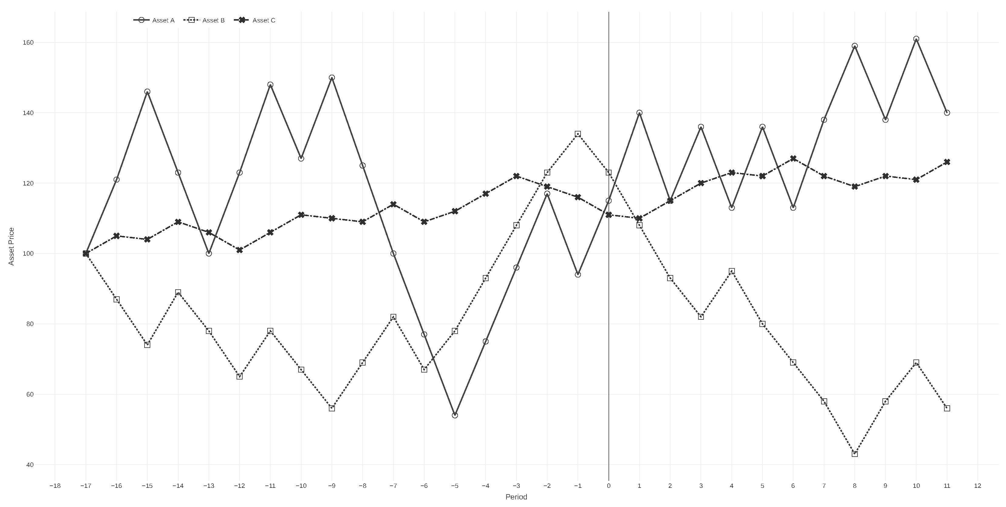
Figure 2.
Portfolio composition by asset and price trend, grouped by blocks of rounds
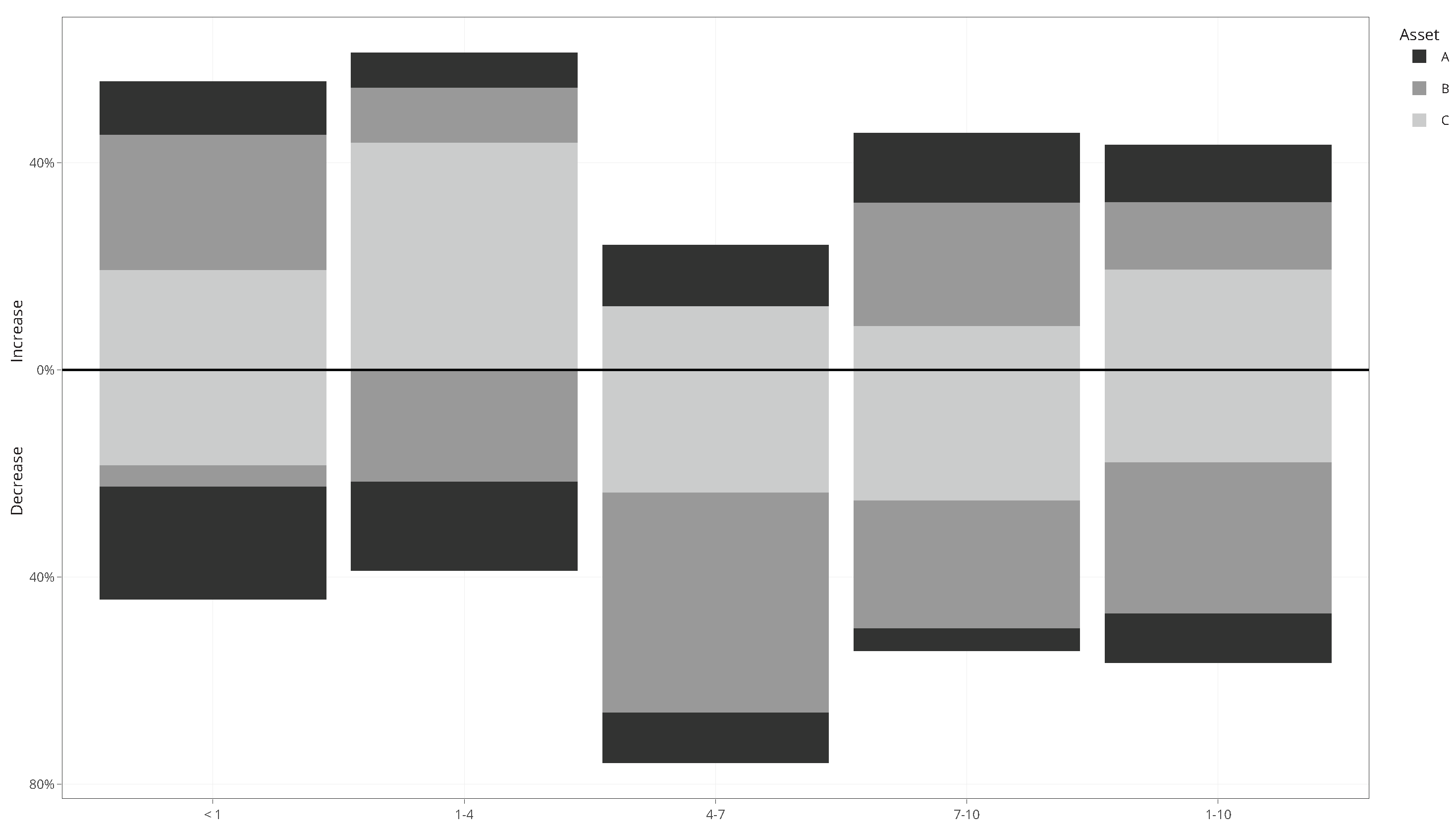

Table 1.
Probability distribution of price changes for each asset (from the initial price of R$ 100)
Table 1.
Probability distribution of price changes for each asset (from the initial price of R$ 100)
| Asset | Increase (+) | Decrease (−) | Possible variation values (R$) |
|---|---|---|---|
| A | 0.5 | 0.5 | 21, 23, 25 |
| B | 0.5 | 0.5 | 11, 13, 15 |
| C | 0.5 | 0.5 | 1, 3, 5 |
Note: Each value has the same probability and is drawn independently (i.i.d.).
Table 2.
Wilcoxon signed-rank test for the average values of both indices
| Rounds | ||
|---|---|---|
| < 1 | 0.27*** | 0.28*** |
| (0.73) | (0.73) | |
| 1-4 | 0.28*** | 0.32*** |
| (0.58) | (0.59) | |
| 4-7 | -0.42*** | -0.41*** |
| (0.57) | (0.60) | |
| 7-10 | 0.14*** | 0.11*** |
| (0.66) | (0.70) | |
| 1-10 | -0.001 | -0.007 |
| (0.68) | (0.70) |
Note: ***, **, *; standard deviation in parentheses.
Table 3.
Number and percentage of assets repurchased after gains and losses, by asset and round
| Rounds | A | B | C | Overall | |||||
|---|---|---|---|---|---|---|---|---|---|
| Total | % | Total | % | Total | % | Total | % | ||
| Gain | <1 | 3522 | 40 | 4095 | 48 | 9475 | 89 | 17092 | 61 |
| 1-4 | 969 | 30 | 1522 | 32 | 7037 | 100 | 9528 | 64 | |
| 4-7 | 1807 | 61 | 0 | 0 | 2117 | 35 | 3924 | 24 | |
| 7-10 | 1846 | 66 | 5765 | 57 | 1823 | 34 | 9434 | 52 | |
| 1-10 | 4622 | 51 | 7287 | 33 | 10977 | 59 | 22886 | 46 | |
| Loss | <1 | 5192 | 60 | 4354 | 52 | 1203 | 11 | 10749 | 39 |
| 1-4 | 2247 | 70 | 3185 | 68 | 0 | 0 | 5432 | 36 | |
| 4-7 | 1151 | 39 | 7107 | 100 | 3973 | 65 | 12231 | 76 | |
| 7-10 | 958 | 34 | 4349 | 43 | 3515 | 66 | 8822 | 48 | |
| 1-10 | 4356 | 49 | 14641 | 67 | 7488 | 41 | 26485 | 54 | |
Table 4.
Number and percentage of assets purchased after price increases and decreases, by asset and round
Table 4.
Number and percentage of assets purchased after price increases and decreases, by asset and round
| Trend | Rounds | A | B | C | Overall | ||||
|---|---|---|---|---|---|---|---|---|---|
| Total | % | Total | % | Total | % | Total | % | ||
| + | <1 | 3704 | 38 | 4384 | 48 | 10133 | 89 | 18221 | 60 |
| 1–4 | 1126 | 28 | 1783 | 33 | 7312 | 100 | 10221 | 61 | |
| 4–7 | 2161 | 55 | 0 | 0 | 2243 | 34 | 4404 | 24 | |
| 7–10 | 2287 | 67 | 6058 | 56 | 2141 | 36 | 10486 | 52 | |
| 1–10 | 5574 | 49 | 7841 | 33 | 11696 | 59 | 25111 | 45 | |
| − | <1 | 6039 | 62 | 4832 | 52 | 1267 | 11 | 12138 | 40 |
| 1–4 | 2869 | 72 | 3600 | 67 | 0 | 0 | 6469 | 39 | |
| 4–7 | 1781 | 45 | 7776 | 100 | 4314 | 66 | 13871 | 76 | |
| 7–10 | 1103 | 33 | 4823 | 44 | 3880 | 64 | 9806 | 48 | |
| 1–10 | 5753 | 51 | 16199 | 67 | 8194 | 41 | 30146 | 55 | |
Table 5.
Average profit of assets sold at any point and of assets kept until the end, by asset and round
Table 5.
Average profit of assets sold at any point and of assets kept until the end, by asset and round
| Rounds | A (R$) | B (R$) | C (R$) | Overall (R$) | |
|---|---|---|---|---|---|
| Kept | <1 | −20.9 | 14 | 13.6 | 7.7 |
| 1–4 | −35.0 | −17 | 21.2 | −12.4 | |
| 4–7 | 32.4 | −50 | −1.6 | −12.9 | |
| 7–10 | 1.9 | −2 | 4.9 | 3.9 | |
| 1–10 | 0.0 | −21 | 7.8 | −6.0 | |
| Sold | <1 | −171.3 | 47 | 15.9 | −54.1 |
| 1–4 | 10.6 | −51 | 18.0 | −7.5 | |
| 4–7 | 38.0 | −87 | −10.8 | −18.3 | |
| 7–10 | −28.9 | 84 | 21.0 | 37.9 | |
| 1–10 | 9.3 | −12 | 9.0 | 3.6 |
Table 6.
Number of sales in period t, conditional on price changes in the two previous periods
| Rounds | Price Trend | Sales | Units Sold | % | |
|---|---|---|---|---|---|
| <1 | U | U | 255 | 3294 | 32.39 |
| D | U | 514 | 3916 | 38.50 | |
| – | U | 769 | 7210 | 70.89 | |
| U | D | 227 | 1571 | 15.45 | |
| D | D | 205 | 1390 | 13.67 | |
| – | D | 432 | 2961 | 29.11 | |
| 1–4 | U | U | 169 | 1235 | 24.92 |
| D | U | 220 | 2122 | 42.83 | |
| – | U | 389 | 3357 | 67.75 | |
| U | D | 147 | 773 | 15.60 | |
| D | D | 141 | 825 | 16.65 | |
| – | D | 288 | 1598 | 32.25 | |
| 4–7 | U | U | 0 | 0 | 0.00 |
| D | U | 282 | 2454 | 44.55 | |
| – | U | 282 | 2454 | 44.55 | |
| U | D | 305 | 2207 | 40.06 | |
| D | D | 109 | 848 | 15.39 | |
| – | D | 414 | 3055 | 55.45 | |
| 7–10 | U | U | 125 | 1430 | 21.22 |
| D | U | 212 | 2901 | 43.04 | |
| – | U | 337 | 4331 | 64.26 | |
| U | D | 157 | 1056 | 15.67 | |
| D | D | 164 | 1353 | 20.07 | |
| – | D | 321 | 2409 | 35.74 | |
| 1–10 | U | U | 294 | 2665 | 15.49 |
| D | U | 714 | 7477 | 43.46 | |
| – | U | 1008 | 10142 | 58.95 | |
| U | D | 609 | 4036 | 23.46 | |
| D | D | 414 | 3026 | 17.59 | |
| – | D | 1023 | 7062 | 41.05 | |
Table 7.
Sales in period t, by whether the current price is above or below the average or maximum observed until
Table 7.
Sales in period t, by whether the current price is above or below the average or maximum observed until
| Rounds | Price Trend | Average | Maximum | ||||
|---|---|---|---|---|---|---|---|
| Sales | Units Sold | % | Sales | Units Sold | % | ||
| <1 | U | 800 | 7341 | 72.18 | 153 | 926 | 10.47 |
| D | 401 | 2830 | 27.82 | 884 | 7920 | 89.53 | |
| 1–4 | U | 389 | 3357 | 67.75 | 26 | 209 | 4.71 |
| D | 288 | 1598 | 32.25 | 580 | 4230 | 95.29 | |
| 4–7 | U | 449 | 3762 | 68.29 | 21 | 219 | 4.35 |
| D | 247 | 1747 | 31.71 | 617 | 4821 | 95.65 | |
| 7–10 | U | 426 | 2962 | 43.95 | 31 | 250 | 4.31 |
| D | 232 | 3778 | 56.05 | 483 | 5556 | 95.69 | |
| 1–10 | U | 1264 | 10081 | 58.60 | 78 | 678 | 4.44 |
| D | 767 | 7123 | 41.40 | 1680 | 14607 | 95.56 | |
Note: The trend is defined relative to the reference values accumulated up to period .
Disclaimer/Publisher’s Note: The statements, opinions and data contained in all publications are solely those of the individual author(s) and contributor(s) and not of MDPI and/or the editor(s). MDPI and/or the editor(s) disclaim responsibility for any injury to people or property resulting from any ideas, methods, instructions or products referred to in the content. |
© 2025 by the authors. Licensee MDPI, Basel, Switzerland. This article is an open access article distributed under the terms and conditions of the Creative Commons Attribution (CC BY) license (http://creativecommons.org/licenses/by/4.0/).
Copyright: This open access article is published under a Creative Commons CC BY 4.0 license, which permit the free download, distribution, and reuse, provided that the author and preprint are cited in any reuse.


