Submitted:
06 May 2025
Posted:
12 May 2025
You are already at the latest version
Abstract
This paper presents methodological advancements to enhance the moving linear (ML)
model approach for time series analysis, with a particular focus on improving model eval-
uation and outlier detection. The ML model decomposes time series data into constrained
and remaining components, allowing for
exible and effective analysis of economic
uctua-
tions. Building on this framework, the extended moving linear (EML) model introduces a
mechanism for outlier detection by treating outliers as parameters estimated via maximum
likelihood. However, challenges remain in providing theoretical support for parameter esti-
mation and ensuring the stable identication of outlier locations. To address these issues,
we rst develop a theoretically grounded evaluation criterion that enables coherent com-
parison of model outcomes. Second, we propose a new outlier detection method based
on maximizing the AIC reduction maximization method, offering a more systematic and
effective approach. Empirical analyses using economic time series data demonstrate the
improved performance and practical utility of the proposed enhancements.
Keywords:
moving linear model approach
; evaluation of model results
; time series component decomposition
; outlier detection
; economic time series
1. Introduction
In [1], a moving linear (ML) model approach was proposed for decomposing time series data into two distinct components. Aimed specifically at business cycle analysis, this approach introduces a novel framework called the constrained-remaining components decomposition. In this framework, the time series is separated into two parts: the constrained component, which is governed by local linear model restrictions and primarily captures the underlying trend, and the remaining component, which is subject to minimal constraints and reflects cyclical movements, irregular fluctuations, and other disturbances in the data.
This separation under mild constraints represents a significant advancement in time series decomposition. While traditional methods typically focus on extracting basic patterns such as trends and cycles, the ML model approach provides a more flexible framework that can be applied across various fields. By employing simple model structures, the ML model achieves both broader applicability and effective handling of diverse data types and analytical objectives. Its ability to decompose time series into constrained and remaining components under flexible restrictions enhances its utility not only in economics but also in other disciplines dealing with temporal data.
A key parameter in the ML model approach is the width of time interval (WTI), which governs the degree of local linearity captured by the constrained component. In [1], WTI is estimated using the maximum likelihood method within a state-space modeling framework, allowing the model to adapt efficiently to local variations in the time series. Accurate estimation of WTI is essential for capturing both short-term fluctuations and long-term trends. In addition, [2] introduced an intuitive, albeit somewhat ad hoc, measure called overall stability to evaluate the performance of the ML model approach, though this measure currently lacks solid theoretical grounding.
Alongside developments in decomposition methods, anomaly detection has recently garnered increasing attention in various research fields, especially in time series analysis (see, [3]). In business cycle analysis in particular, identifying unexpected values or abrupt fluctuations is crucial. Numerous detection methods have been proposed (see e.g., [4]; also references therein), but many are highly specialized. For example, [5] evaluated three statistical outlier detection algorithms for water surface temperature using an unsupervised method. While valuable, these methods often lack general applicability. In the context of ML modeling, [6] proposed a two-step approach combining time series decomposition and anomaly detection. However, this procedure remains somewhat ad hoc and complex.
Building upon the ML model framework, [7] proposed an extension known as the extended moving linear (EML) model, which incorporates a robust method for outlier detection and estimation. In this extended framework, outliers are treated as parameters, with both their number and locations simultaneously estimated using the maximum likelihood method. Model selection is guided by the Akaike Information Criterion (AIC), enhancing the precision of outlier identification. To improve the search for outlier locations, [7] introduced a heuristic but practical procedure, addressing the challenge of accurately identifying irregular points in time series data. This extension significantly improves applicability to real-world economic data, where outliers – such as those from financial crises or global pandemics – can distort analytical results. Nevertheless, while the EML approach provides a well-structured detection method, it remains somewhat ad hoc, and its performance may be unstable due to the neglect of interrelationships among outliers.
The aim of the present chapter is twofold. First, we focus on reinforcing the ML model approach. While the use of maximum likelihood estimation for determining the WTI presents no particular difficulties, it is inherently model-dependent. Our goal is not merely to justify this approach, but to provide theoretical support for both the modeling framework and its estimation method through a logical and systematic discussion. We also propose a new evaluation criterion that offers a theoretically coherent and practically useful basis for assessing model performance. Second, we aim to refine the EML model approach for outlier detection by proposing a new method based on the maximization of AIC reduction. This approach identifies outliers based on their contribution to AIC improvement, offering a more systematic and effective detection framework.
Through these developments, we seek to enhance the robustness and practical utility of both the ML and EML model approaches. In particular, we aim to improve their performance in analyzing economic time series, where business cycles and outlier events pose significant analytical challenges. By introducing refined methods for model evaluation and anomaly detection, we aim to enable more reliable application of these models to real-world data. To support these methodological advancements, the state-space model-based decomposition approach proposed by [8] serves as a valuable reference point.
The remainder of this paper is organized as follows. Section 2 reviews the ML and EML model approaches. Section 3 introduces new developments aimed at reinforcing these approaches. Section 4 presents empirical examples to illustrate the analytical procedures and demonstrate the effectiveness of the proposed enhancements. Finally, Section 5 provides a summary and discussion.
2. A Review of the ML and EML Model Approaches
This section provides a comprehensive review of the Moving Linear (ML) model approach proposed by [1] and its extension, the Extended Moving Linear (EML) model approach introduced by [7]. These approaches serve as the theoretical foundation for the methodology developed in the present study.
2.1. The ML Model Approach
We begin by reviewing the ML model approach as presented in [1].
2.1.1. The Basic Model
We consider decomposing a time series into two unobserved components as follows:
where and represent the constrained and remaining components, respectively. Here, t is the time index, and N is the sample size. The constrained component reflects long-term variation, typically smooth, while the remaining component captures short-term variations, such as cyclical fluctuations.
To ensure smoothness for the constrained component, we use a linear model of time t:
Here, k is the width of the time interval (WTI), and and are the coefficients in this interval. The n-th time interval is defined as for . A centered time variable within the n-th interval is introduced as follows:
where is the midpoint of the time interval.
Substituting into the model in Eq. (2) gives:
where . The model in Eq. (1) then becomes:
which is referred to as the moving linear model (ML model).
2.1.2. State Space Presentation of the ML Model
In the ML model in Eq. (3), the quantities , , and are treated as parameters. To achieve stable parameter estimates, we introduce the following priors for these parameters.
Firstly, it is assumed that and vary smoothly with respect to n as follows:
under diffuse priors for and . Specifically, it is assumed that and , where the variance is set to a sufficiently large value.
Moreover, to uniquely identify the remaining component locally, the following prior distribution for and is introduced to probabilistically maintain the orthogonality relationships between and , as well as between and in the n-th time interval:
To express the transition relationships, the priors for the other remaining component terms are given as:
In these equations, represent a set of system noises, where it is assumed that i.i.d., with , and is an unknown parameter.
Bayesian form of the ML model was constructed based on the above settings.
Then, under the settings
a state-space representation for the moving linear model can be defined as
with , where .
Therefore, given the initial conditions and , and the observations , we can compute the mean vectors and covariance matrices of the state variable for using the Kalman filter and fixed-interval smoothing algorithms, as described below (for details, see [1,9]):
[Kalman filter]
[Fixed-interval smoothing]
Using the above procedure, component decomposition can be performed. In particular, by incorporating for into the state vector (for ), the remaining component can be estimated within this model framework. The posterior distribution of the state vector obtained from fixed-interval smoothing is Gaussian, with mean and covariance matrix . Accordingly, the estimate of can be extracted from for , and the estimate of the constrained component is obtained as .
2.1.3. Method for Estimating the Parameters
In the setup described above, the WTI, k, and the variance of the system noise are the key parameters that characterize the ML model.
According to [8], based on the Kalman filter, the density function of the predictive distribution of is expressed in the form of a normal distribution:
with
where and are the mean and covariance matrix of the predictive distribution of , given by:
Here, and are the mean and covariance matrix of the state in the prediction step of the Kalman filter.
To define the likelihood as the product of conditional probability distributions, it is necessary to structure the vectors and matrices related to the observation vector as follows. Specifically, , , , and are expressed as:
with a being a scalar and a vector of appropriate dimension.
In this case, the density function of is expressed as:
with
where
Thus, for , the joint density function of is given by . For , the conditional density function of given is expressed as:
Moreover, the joint density function of is expressed as:
When the observed values of are given, the function becomes the likelihood function for and k. Thus, the log-likelihood function is given by:
Therefore, when k is given, the log-likelihood function defined in Eq. (11) can be maximized to obtain the estimate of . However, this optimization problem is difficult to solve analytically and generally requires numerical optimization methods.
Further, if is temporarily set to 1 in the Kalman filter, the maximum likelihood estimate of can be obtained analytically as:
Finally, the conditional log-likelihood function with respect to k, denoted as , is a function of k alone. Therefore, the estimate of k can be obtained by maximizing .
2.2. The EML Model Approach for Outlier Detection
Below, we provide another review of the EML model approach, based on [7].
2.2.1. The Basic Model
Within the framework of the ML model approach, the following model is introduced to handle cases in which the time series contains outliers:
where represents the unusually varying component of the time series, which may include outliers. The other variables and associated assumptions in Eq. (12) are consistent with those in Eq. (1).
As a basic assumption, we suppose that the full dataset contains m outliers, denoted by , with . If an outlier is present at time t, the corresponding unusually varying component is assigned one of the values from . If no outlier is present at time t, is set to zero. In other words, within the set , exactly m elements correspond one-to-one to the elements in the outlier set , while the remaining elements are zero.
Therefore, a simple setting for handling outliers can be employed (see [7]). Specifically, let denote the vector of outliers. We consider as a set of functions of the outliers , where each is treated as an unknown constant. By defining , the transformed dataset becomes a version of the data with outliers removed. Applying in place of to the ML model approach, the log-likelihood defined in Eq. (11) becomes a function of , enabling estimation via the maximum likelihood method.
While this setting is simple and intuitive, when m is large, it leads to high computational costs and may compromise the reliability of the estimation results.
2.2.2. Bayesian Approach to Outlier Estimation
To address the presence of multiple outliers in a more general framework, a Bayesian approach is introduced as follows.
In this framework, outliers are formally treated as time-varying random variables. Specifically, each outlier is represented as , and a transition equation is defined as
which assumes that each outlier remains constant over time at step n.
By incorporating Eq.(4), (5), and (6), a Bayesian model is constructed for the EML model, with Eq.(7) and (8) are redefined as follows:
where denotes an m-dimensional identity matrix, denotes a zero matrix with appropriate dimensions, and is a concatenation function defined such that if for some , and otherwise, for .
Then, under the setting , the state space presentation for the Bayesian EML model can be expressed using Eqs. (9) and (10).
Based on the above formulation and by applying in both the Kalman filter and fixed-interval smoothing algorithms, estimates of the state vector can be obtained. Consequently, the estimates for the outliers, as well as the estimates of the remaining components, can be extracted from for . Specifically, corresponds to the elements from the -th to the -th entries in the vector , which depend only on the smoothing result at . The corresponding variances of the outlier estimates are given by the diagonal elements of the covariance matrix from the -th to the -th rows.
2.2.3. Outlier Detection and Estimation
The key steps for identifying the positions of outliers and estimating their values are as follows. First, ignoring the presence of outliers, the time series is decomposed into constrained and remaining components using the ML model approach. The initial outlier positions are then set as the time points corresponding to the top m values of the remaining component in terms of their squared magnitudes.
Next, the EML model provides Bayesian-type estimates of the outliers, which approximate maximum likelihood estimates. These estimates enable the computation of an approximate maximum log-likelihood, which in turn allows the number of outliers to be determined using the minimum AIC criterion.
Subsequently, the estimated values of the outliers are normalized by their standard deviations. By ranking the normalized squared estimates, a new set of outlier positions is obtained. This update distinguishes the revised positions from the initial setting and enables more accurate estimation based on the updated locations. The procedure for updating outlier positions is repeated iteratively until the estimation results converge.
Although the final step is well-structured, it remains somewhat ad hoc, and its performance in detecting outliers is unstable due to the lack of consideration for interrelationships among outliers. Revising this step is a central objective of the present study.
3. New Development to Reinforce Previous Findings
3.1. The Aims
In the current ML model approach, the WTI is estimated using the maximum likelihood method. From the perspective of statistical analysis, the use of maximum likelihood itself poses no particular issues. However, as maximum likelihood estimation is inherently model-dependent, our aim is not merely to justify its application but to provide theoretical support for both the model and the estimation method through logical and systematic discussion. In particular, we seek to develop a theoretical understanding of the critical role that WTI plays in improving the model’s overall performance.
Although WTI was originally introduced as a practical device, we endeavor to clarify, from a theoretical standpoint, how it facilitates the effective separation of constrained and remaining components and contributes to the stabilization of subsequent estimation procedures. This theoretical elaboration is essential for reinforcing the model’s interpretability and robustness.
In addition, when comparing different estimation methods, likelihood values are not always a reliable basis due to fundamental differences in model structure. To address this issue, another key objective is to propose new evaluation metrics based on the variance-covariance structures of the decomposed components. These metrics are intended to enable a more holistic assessment of the decomposition results and thereby enhance the credibility of the ML model approach. Unlike existing methods that rely narrowly on likelihood, the proposed metrics capture a wider range of estimation characteristics and offer a theoretically sound and practically useful basis for model comparison and evaluation.
Furthermore, as noted in Section 2.2.3, while the existing EML approach for identifying outlier positions is well-designed, it remains somewhat ad hoc and can exhibit unstable performance due to its neglect of the interrelationships among outliers. To address these limitations, we propose a method based on the maximization of AIC reduction, which identifies outliers by evaluating their individual contributions to the decrease in the AIC. This approach selects outlier positions that most significantly enhance model fit. By introducing this theoretically grounded and computationally efficient method, the outlier detection process becomes more stable, systematic, and reliable.
Collectively, these enhancements-clarifying the theoretical role of the ML approach, proposing additional evaluation metrics, and refining the outlier detection process-represent significant steps toward completing and strengthening the ML and EML model approaches as a coherent and reliable framework for time series analysis.
3.2. Reinforcing the ML Model Approach
In this section, we aim to reinforce the ML model approach by offering theoretical insights into the evaluation of results and by proposing additional evaluation metrics.
3.2.1. Variance-Preserving Adjustment of the Decomposed Components
Within the context of the ML model approach, the constrained-remaining decomposition yields and as the decomposed constrained and remaining components, respectively, such that the original time series can be represented as:
Obviously, the decomposition in Eq. (13) is average-invariant, ensuring that the equality holds, where
denotes the average of the time series , and and denote the averages of the constrained and remaining components, respectively. Note that in the ML model approach, the remaining component is adjusted so that becomes zero. As a result, is equal to the average . This implies that the average level of the constrained component matches that of the original time series.
In addition to the average-invariance of the decomposition in Eq. (13), variance-invariance is also desirable; however, it cannot be consistently maintained by the ML model approach. Let denote the sample variance of , while and denote the sample variances of and , respectively, and let denote their sample covariance. Then, the following relationship holds:
If , indicating no correlation between the decomposed components, then we have
Thus, the decomposition becomes variance-invariant, meaning that the total variance of the original time series equals the sum of the variances of the decomposed components without any covariance term.
In the ML model approach, the decomposed components are generally uncorrelated due to the model specification. However, this property may vary depending on the parameter settings and the characteristics of the data. When a correlation exists between the components, an adjustment can be made to restore variance-invariance by introducing the following regression model:
where is the centered constrained component, is the regression coefficient, and is the residual term.
Based on the least squares estimate of , the remaining component can be adjusted as follows:
where represents the adjusted remaining component, which can be used as the final decomposed result.
By the orthogonality property of least squares estimation, is uncorrelated with , thereby ensuring that variance-invariance is preserved when is used as the final decomposed result in place of . This adjustment, which renders the decomposed components uncorrelated, is referred to as a variance-preserving adjustment.
Incidentally, as shown in Eqs. (15) and (16), the variance-preserving adjustment effectively eliminates the portion of the remaining component that is correlated with the constrained component, while maintaining the smoothness of the latter. Although an alternative method of achieving variance preservation – namely, adjusting the constrained component based on the remaining component – is theoretically possible, it is not recommended because it may compromise the smoothness of the trend.
Through the variance-preserving adjustment, the ML model approach can maintain the invariance properties of the constrained-remaining decomposition, namely, both average-invariance and variance-invariance. In statistical data, information is primarily conveyed through variance; thus, ensuring variance-invariance guarantees the preservation of information content before and after decomposition.
3.2.2. Structural Examination of Variances for the Decomposed Components
As discussed in the previous section, the variance-preserving adjustment ensures the maintenance of the variance-invariance property in the constrained-remaining decomposition, as shown in Eq. (14). As a result, for a given time series , the total variance of the two decomposed components remains constant, as expressed by the following equation:
To further investigate the relationship between the decomposed components, define the product of their variances as
It can be confirmed that PV reaches its maximum when the variances of the decomposed components are equal, that is, when . In this case, by also referring to Equation (17), it becomes clear that , and the maximum value of PV is given by .
On the other hand, when the WTI, k, is small, the constrained component absorbs a large part of the fluctuations of the time series, exhibiting large variability. As a result, the remaining component contains relatively small fluctuations, leading to
As k increases, decreases and increases, so that gradually becomes smaller. Thus, the product of variances, PV, behaves as a monotonically non-decreasing function with respect to k.
When k continues to increase, and eventually become equal, so that PV reaches its maximum value. Beyond this point, as k increases further, PV becomes a monotonically non-increasing function of k.
When attempting to extract information related to business cycle fluctuations from time series data, such information is often captured by the variations of the remaining component. Therefore, it is natural to expect that the variance of the remaining component will be large in such contexts. Based on this expectation, one might consider choosing a larger value of the parameter k – particularly when starting from a small k – in order to achieve a higher value of PV and thereby better capture cyclical variations.
However, such an approach cannot be adopted indiscriminately. The structure of the model imposes constraints that must be respected. Simply increasing k in an attempt to maximize PV without regard to these structural constraints may lead to decompositions that are inconsistent with the fundamental assumptions of the model.
In summary, the absolute value of PV itself cannot be directly used as a criterion for evaluating the quality of a decomposition result. Nevertheless, PV serves as an important indicator of the relationship between the characteristics of the time series data and the parameter k. Therefore, for a given dataset, rather than focusing on the absolute magnitude of PV, it is more meaningful to observe how PV varies with k.
3.2.3. Assessing the Stability of Structural Changes in Decomposed Components
While the previously introduced indicator PV captures the relative changes in the variances of the two components as the parameter k varies, it does not reflect the internal stability or continuity of each component across successive values of k. In other words, PV illustrates how the variances of the constrained and remaining components, and , change in relation to each other, but it does not indicate whether the structural changes within each decomposed component occur gradually or abruptly as k increases.
To address this limitation, we consider an alternative approach that evaluates the similarity of each component’s decomposed results with respect to a unit change in the successive value of k. This similarity can be quantified using the covariance between the decomposed results at the two settings. Specifically, for the constrained component, let and denote the decomposed results obtained at and k, respectively. Instead of using the variance , we introduce the covariance between and as an alternative indicator. If the decomposed results change only slightly with respect to k, the covariance will be close to , suggesting that the component remains stable as k increases.
A similar argument applies to the remaining component. Instead of using the variance , we apply the covariance between and , which denote the decomposed remaining components obtained at and k, respectively.
Building upon this idea, we propose an extended measure analogous to PV that incorporates both the relative changes in variance between the two components and the degree of continuity within each component across successive values of k. Specifically, by replacing and with and , respectively, we define an extended indicator that simultaneously captures both the inter-component variance relationship and the intra-component consistency with respect to k. This combined measure provides a more comprehensive understanding of the decomposition behavior, particularly in applications where both smooth transitions and balanced variance allocation are critical considerations.
Moreover, for the constrained component, let denote a decomposed result obtained using a different method, and let denote the result obtained using the ML model approach with a fixed value of k. We use the covariance between and as a measure of similarity between these two results. A similar approach can be applied to the remaining component. Therefore, by integrating both aspects, we can compare the similarity between the decomposition results obtained by a different method and those from the ML model approach, with reference to the values of k.
The above concept serves as a useful basis for constructing indicators to evaluate decomposition results. From this perspective, a set of decomposed results obtained at a value of k that induces smaller fluctuations in the indicator can be regarded as reflecting a more stable underlying structure. Accordingly, it is preferable to adopt the decomposition corresponding to such a value of k, as it is likely to provide a more reliable representation of the time series structure. Furthermore, similar indicators can be developed to facilitate comparisons with alternative decomposition methods.
3.2.4. Evaluation Metrics for Assessing Decomposition Stability
In the constrained-remaining decomposition, evaluating the stability of the results is essential for understanding the underlying structure of a time series. One type of indicator for such evaluation is an extension of the product of variances. Since this indicator varies with the parameter k, it potentially reflects the structure of the decomposed results. However, it may exhibit unstable behavior depending on the characteristics of the time series and the chosen decomposition framework. This section discusses a more robust evaluation strategy based on the extended product of variances and explores its relationship to both likelihood-based estimation and alternative decomposition methods.
Building on the previous discussion, we define the Index of Structural Similarity (ISS) by extending the product of variances (PV) as follows:
where k is the parameter of interest, and all terms are defined in the previous sections. This formula incorporates dimensional adjustment and is based on the observation that the maximum of can approach , so the ISS may take values close to 1.
The measures the overall similarity of the decomposition results before and after an increase in k. A decrease in ISS suggests that the decomposition results change abruptly as k increases.
Furthermore, for a given value of k, the similarity between the components obtained by a different method — namely, and — and those from the ML model approach can be evaluated by replacing and with and in the ISS formula in Eq. (18). We refer to this kind of index of structural similarity as the mutual index of structural similarity (MISS).
However, may exhibit unstable behavior depending on the characteristics of the time series. Thus, based on , we define an index of instability (IOI) as
As shown in Equation (19), is defined as the difference in the logarithm of with respect to k, and thus serves as a measure corresponding to the rate of increase of with respect to k. A small indicates that changes gradually as k increases. This suggests that the decomposition structure is relatively invariant with respect to k. Hence, the value of k corresponding to a small magnitude of may be selected as the most structurally stable decomposition point. Therefore, can be used, along with the likelihood, as a reference indicator for determining the value of k and evaluating the estimation method.
3.2.5. Bidirectional Processing and Recursive Decomposition Strategies
The original ML model approach is processed in the order of , and the component decomposition is conducted according to this order. This is referred to as forward processing. On the other hand, it is referred to as backward processing if the same model is configured with the component decomposition proceeding in reverse order, that is, . Since the correspondence between decomposed results and observations differs between the forward and backward processings, the results of component decomposition may also differ.
By averaging the estimation results at the same time point obtained from these two processings, a more stable and accurate component decomposition can be achieved. In other words, integrating the results obtained through bidirectional estimation – namely, the forward and backward processings – can provide more reliable and robust outcomes compared to estimation based solely on forward processing.
It should be noted that the constrained-remaining components decomposition is not necessarily completed in a single step. If necessary, the ML model approach can be repeatedly applied to the resulting components to further decompose a given component into two or more subcomponents. However, the interpretation and utilization of such decomposition results should be carefully determined in accordance with the characteristics of the data under analysis and the objectives and context of the application.
Moreover, [1] proposed an orthogonalization method to transform the resulting components into mutually uncorrelated time series when multiple components are obtained.
3.3. Reinforce the EML Model Approach
In this section, we aim to refine the method for determining the locations of outliers to reinforce the EML model approach.
3.3.1. Outlier Detection and Estimation
The original problem involves identifying and estimating m outliers within a sample dataset of size N, where m is much smaller than N. This task presents a combinatorial challenge and is therefore considered a significant endeavor. To address this issue, it is crucial to obtain some indication of the potential positions of the outliers.
For the sake of completeness, the full system enhanced in this study is presented below. Notably, the third step constitutes a novel contribution of this work.
- (1)
- Determining the potential Positions of Outliers
When we do constrained-remaining decomposition using the ML model approach with a large WTI , most of the outliers become assimilated into the estimate of the remaining component. Thus, the estimates for the remaining component can be used as references. That is, we can assume that
Let represent an observation from the random process , and let be the realized value for a random process , where , and is assumed to contain a potential outlier. It is further assumed that and . The expected value can be expressed as follows:
Thus, we have
This suggests that becomes particularly large when may contain an outlier. Additionally, when , provides an unbiased estimation of .
In summary, a large is likely to contain . When considering the number of potential outliers as m, if , it is reasonable to infer that contains the largest outlier in amplitude, contains the second-largest outlier, and so on. In other words, one can establish the order for searching potential outlier positions as . Subsequently, the positions of the outliers can be determined based on this order.
- (2)
- Estimation of Outliers and Their Number
Assume that for a given integer M and a vector of potential outliers , a subvector consisting of m elements selected from is incorporated into the model for . When the positions of outliers are determined (though they may be tentative), applying the extended ML model approach yields a Bayesian-type estimate for the outliers. This estimate is a form of maximum a posteriori probability, closely approximating the maximum likelihood estimate. Therefore, the estimates can be substituted into in as an approximation of the maximum likelihood , which is defined in Eq. (11).
This allows for an approximate calculation of the maximum log-likelihood, and based on that, the defined by
which depends on the value of m. Thus, the estimation of the number m of outliers using the minimum AIC method (see [10]).
- (3)
- Updating the Outlier Positions
Based on the potential setting of outlier locations in sequential order, we estimate the parameters for each model corresponding to the number of outliers , and compute the corresponding values of using Eq. (20). Specifically, the case of assumes that no outliers are present; assumes that a single outlier exists at time ; assumes that outliers exist at times and ; and so forth. In this manner, we obtain the following sequence of AIC values:
Next, based on the AIC sequence in Eq. (21), we construct the sequence of AIC differences defined by , as follows:
Within the sequence of AIC differences given in Eq. (22), any time point associated with an index i such that can be considered to have special significance. That is, incorporating an additional outlier at time , on top of the outliers already introduced at , leads to a decrease in the AIC value, which implies an improvement in model fit. Therefore, such an outlier can be regarded as the i-th outlier that should be included in the model.
This reasoning allows us to update the outlier locations. Specifically, we examine the sequence of in Eq. (22) in ascending order. For instance, if the AIC difference corresponding to outlier number is the smallest, we update the location of the -th outlier to the corresponding time point . Similarly, if is the second smallest, we update the location of the -th outlier to the corresponding time point . In this way, we update the previous setting of outlier locations to the following:
We refer to the sequence in Eq. (23) as the updated outlier locations.
Once this update of outlier locations is performed, the updated set is used as a new setting, and the procedure of replacing outlier positions is repeated. In theory, this iterative process continues until the updated outlier locations coincide with the previous setting. However, from a practical perspective, it is generally sufficient if the elements contributing to negative DAIC can be identified in a stable manner before and after the update.
Ultimately, including outliers in the model that lead to negative DAIC differences results in a lower AIC value and, consequently, a better-fitting model. Thus, through this process, the number of outliers to be included in the model is determined automatically. Specifically, if the first outliers in the updated sequence of Eq. (23), up to , all result in negative values of , then the outliers at the corresponding time points should be incorporated into the model. In doing so, we obtain the optimal model corresponding to the minimum AIC.
We shall refer to the aforementioned method of determining the locations and number of outliers as the AIC reduction maximization method. This method takes into account the dependencies among outliers and constitutes the next significant contribution of this study.
4. Empirical Examples
4.1. Empirical Analysis of Capital Investment in Japan
The first empirical example analyzes business expenditures for new plant and equipment (BE) in Japan. The goal of this example is to demonstrate the analytical procedure and highlight the effectiveness of the reinforcement in the ML model approach.
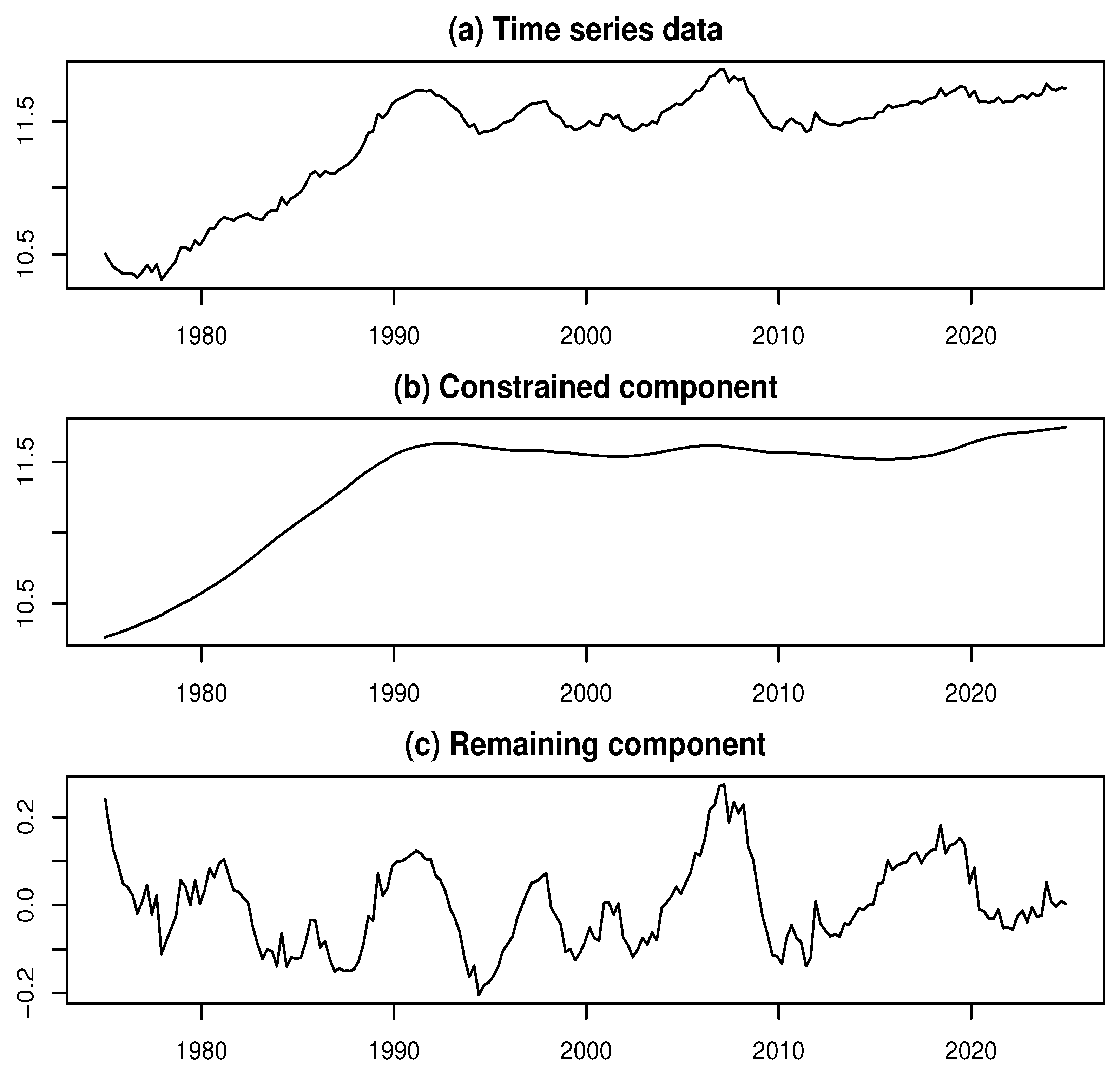
The time series of BE reflects levels of capital investment and is known for exhibiting distinct structural characteristics. The original BE data were obtained from the website of the Japanese Cabinet Office (see [11]). The data constitute a monthly time series spanning from January 1975 to December 2024, amounting to observations. Figure 2a displays a plot of the logarithmically transformed BE series (log-BE).
We applied the ML model approach to decompose the log-BE time series, performing the decomposition for each value of k ranging from 3 to 202. As shown in Figure 1a, the log-likelihood (LL) exhibits local maxima at three values of k: 47, 111, and 152, corresponding to LL values of 3867.97, 3905.51, and 3936.1, respectively. Among these, the highest LL is achieved at , which is adopted as the estimate of k. Furthermore, Figure 1b indicates that the IOI reaches its minimum around . These findings suggest that the maximum likelihood estimate of k effectively captures a stable underlying structure.
Figure 2b,c illustrate the decomposed results for the log-BE time series, with Figure 2b depicting the constrained component and Figure 2c representing the remaining component.
Figure 2.
Data and decomposed results for the log-BE time series
Incidentally, to validate the results of this study, we refer to the state-space modeling approach introduced in [8]. In that work, the R function season is employed to decompose a time series into three components: a trend component, an AR component, and observation noise. When this function was applied to the log-BE series, the order of the trend component was estimated to be 2, and that of the AR component was estimated to be 4. Based on these estimates, the time series was decomposed accordingly.
To align with the ML model framework, we treated the trend component as the constrained component and considered the combined AR component and observation noise as the remaining component. For each value of k, we computed the MISS values by comparing the decomposition results from the ML model approach with those obtained using the season function. The MISS reached its minimum around , suggesting that the conventional state-space-based decomposition closely corresponds to the ML model approach at this value of k. Notably, around , the IOI value is approximately 0.08, which is near its maximum. This implies that the conventional component decomposition using the state-space model lacks stability.
These findings suggest that the constrained component produces a highly smooth time series, effectively capturing the long-term trend in log-BE. Consequently, most short-term fluctuations are absorbed into the remaining component, which exhibits complex and irregular behavior. This observation provides a strong rationale for reapplying the ML model approach to further decompose the (first) remaining component.
Thus, we further decomposed the log-BE time series for each value of k ranging from 3 to 182. As shown in Figure 3a, similar to the first component decomposition, the LL exhibits local maxima at three values of k: 47, 111, and 155, corresponding to LL values of 3853.70, 3814.70, and 3937.52, respectively. Among these, the highest LL is achieved at .
However, as shown in Figure 3b, the IOI values at these k points are elevated compared to their surroundings, suggesting that the most stable decomposition may not be achieved at these values. A closer examination of Figure 3b reveals a noticeable dip in the IOI at . Although the LL value at this point, 3719.58, is not exceptionally high, the LL values in its vicinity remain relatively stable at a high level. Therefore, is adopted as the estimate of k for the second component decomposition.
Figure 4 displays the results of the second decomposition applied to the remaining component obtained from the first decomposition. Figure 4a,b show the constrained and remaining components, respectively.
The constrained component in the second decomposition, shown in Figure 4a, exhibits cyclical behavior with a period of over a decade, aligning with the Juglar cycle. This point deserves emphasis: in this case, the time series subject to decomposition is itself a remaining component containing cyclical fluctuations of varying periods. Consequently, the constrained component extracted through this process captures a long-period, highly smooth cyclical fluctuation.
Furthermore, the remaining component in the second decomposition, shown in Figure 4b, is characterized by short-term cyclical fluctuations. These findings reinforce the consistency of the results with business cycle theory and underscore the effectiveness of the proposed approach in identifying and analyzing economic cycles (see [1]).
The results presented above suggest the following: by incorporating additional metrics and estimation methods alongside the conventional maximum likelihood approach, more stable decomposition results can be achieved. Naturally, different decomposition outcomes may arise depending on the number of components extracted and the choice of k values. This underscores the fact that data analysis is inherently both data-driven and purpose-driven; thus, trial and error, guided by the analytical objectives of the data under investigation, is essential.
4.2. Empirical Analysis of Industrial Production in Japan
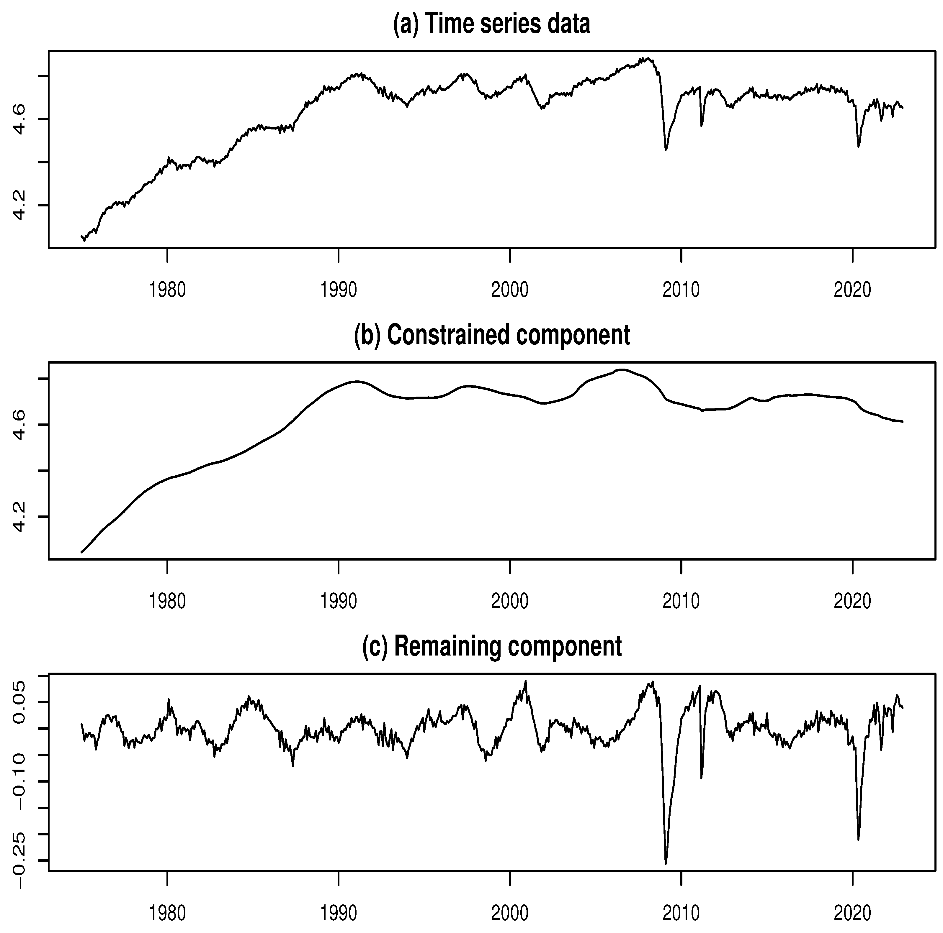
In this section, we present an empirical analysis of the seasonally adjusted index of industrial production (SAIIP) in Japan as a second example. This example demonstrates the effectiveness of the reinforced EML model approach in detecting and estimating outliers in time series data.
The SAIIP data were obtained from the same source as the BE data. As SAIIP serves as a principal indicator for analyzing economic trends, it is frequently used in empirical studies. Due to its sensitivity to sudden changes in economic conditions, outliers tend to appear frequently.
To facilitate comparison with the empirical example in [7], we use the data as a monthly time series from January 1975 to December 2022, comprising a total of months. A logarithmic transformation is applied to the SAIIP time series, which we refer to as log-SAIIP. The objective is to analyze the time series behavior of log-SAIIP.
Figure 6a presents the time series plot of log-SAIIP. Two prominent declines are clearly observable in the series. The first, occurring around February 2009, is attributable to the aftermath of the 2007–2008 global financial crisis. The second, around May 2020, reflects the impact of the COVID-19 pandemic. These sharp drops are likely to be associated with the presence of multiple outliers.
We applied the ML model approach to decompose the log-SAIIP time series, performing the decomposition for each value of k ranging from 3 to 202. As shown in Figure 5a, the log-likelihood (LL) exhibits three prominent local maxima at , , and , corresponding to LL values of 4285.37, 4555.44, and 4601.83, respectively. Furthermore, at , the LL shows a spike-like surge, reaching a peak value of 4453.67. A closer examination of Figure 5b reveals a noticeable dip in the IOI at , which corresponds to the first local maximum of the LL. Although the LL at this point is not the global maximum, the surrounding LL values remain relatively stable at a high level. Therefore, for the purpose of comparison with the findings of Kyo (2025b), and based on the above observation, we adopt as the estimated value of k for the second component decomposition.
Figure 6b,c present the results of the constrained-remaining component decomposition using the ML model approach with . In Figure 6b, the constrained component exhibits a smooth trend, while Figure 6c shows that the remaining component displays cyclical variations, indicating the presence of business cycles in Japan. Notably, a substantial portion of the sharp declines observed around February 2009 and May 2020 can be attributed to the remaining component. These abrupt drops in the time series are likely to reflect the influence of outliers caused by sudden economic shocks. Therefore, the elements associated with these variations should be identified and treated as outliers, as they may distort the analysis of business cycles.
Figure 6.
Data and decomposed results for the log-SAIIP time series
The upper bound for the number of potential outliers was set to , and the potential locations of the outliers were determined based on large squared values in the decomposed remaining component time series.
Furthermore, based on the AIC reduction maximization method, the number of outliers was estimated as , with the minimum AIC value being . The estimated outlier positions are at time points 410, 411, 545, 412, 413, 409, 414, 546, 547, 415, 416, 436, 435, 548, 544, 408, 149, 398, 401, 399, 397, 394, 400, and 403. Arranged in chronological order, these positions mainly correspond to the periods from December 2008 to August 2009 and from April 2020 to July 2020.
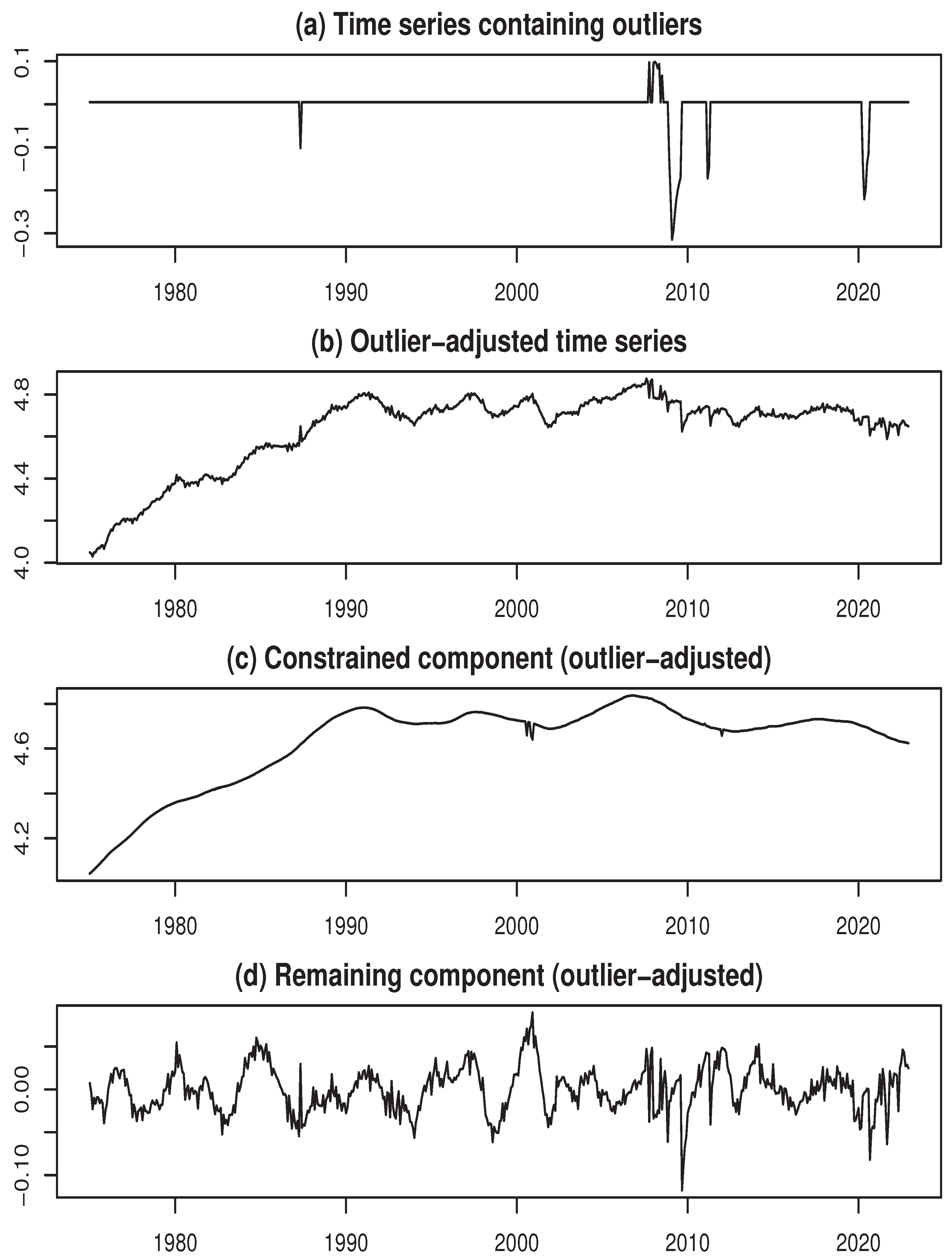
Finally, we performed the estimation of outliers using . Figure 7a depicts the time series containing outliers, Figure 7b displays the final outlier-adjusted time series, while Figure 7c,d show the estimates of the constrained and remaining components for the outlier-adjusted time series. It can be confirmed that, compared to the initial estimate of the remaining component in Figure 6c, the estimation results with the outlier-adjusted data in Figure 7d show a significant improvement in uniformity.
As a reference for comparison, we again present the main results obtained in [7]. In [7], we used an EML model approach, which is reviewed in Section 3.3, for detecting and estimating outliers. The number of outliers was estimated as based on the method of determining outlier locations according to the order of the squared standardized outliers, resulting in a minimum AIC value of . The outlier positions were estimated at the following time points: 410, 411, 412, 413, 409, 414, 415, 435, 416, 545, 436, 546, 408, 149, 547, 544, 398, 394, 397, 399, 401, and 548.
Thus, by updating the method for detecting outliers, the AIC decreased by 789.62, thereby improving the reliability of the estimation results. As a result, two additional outliers were detected. These newly added outliers are active at time points 400 and 403, corresponding to April and July of 2008, respectively. The marginal contributions to the AIC reduction for each are 13.43 and 17.53, respectively. The difference between the component decomposition results obtained in [7] and those shown in Figure 7 is not easily visually discernible in the graph, so it will be omitted. However, as described below, a comparison based on the numerical values of the evaluation metrics is possible.
Therefore, we evaluate the decomposition results using the index of symmetry and uniformity (ISU), proposed by [12], as a benchmark. For a given time series, the ISU is defined as the logarithmic ratio of the standard deviation of the series’ absolute values to the standard deviation of the original series. For the outlier-adjusted remaining component, a larger standard deviation of the absolute values indicates a smoother outlier-adjusted constrained component. This suggests that the influence of outliers on the decomposition result is weaker, leading to greater stability, which is desirable. Conversely, a smaller standard deviation of the absolute values implies greater symmetry around the mean and also a weaker influence of outliers on the remaining component – another desirable outcome. Therefore, the decomposition results can be evaluated using the minimum ISU criterion applied to the outlier-adjusted remaining component.
The following results were obtained based on the above findings. For the result derived from the method proposed by [7], the ISU was , whereas for the result based on the present AIC reduction maximization method, the ISU decreased to . This demonstrates the advantage of the AIC reduction maximization method in updating conditions, as evaluated by the minimum ISU principle.
Considering these outcomes, a key feature of the proposed method is its thorough implementation of the ML model approach, which makes it particularly promising for handling outliers in the decomposition of constrained and remaining components.
5. Summary and Discussion
We began by reviewing the moving linear (ML) model approach proposed by [1], along with its extension, the extended moving linear (EML) model introduced by [7], which together form the theoretical foundation of this study. Building on these frameworks, we introduced several methodological advancements, particularly focusing on improving outlier detection and estimation.
Although WTI was initially developed as a practical tool, we clarified its theoretical significance in separating constrained and remaining components, thereby contributing to the stability of estimation and enhancing both the interpretability and robustness of the model. To support model evaluation, we also proposed new metrics that offer a broader perspective than traditional likelihood-based methods. A core contribution is the index of instability (IOI), constructed from the index of structural similarity (ISS), which serves as a powerful supplementary criterion to the log-likelihood and reinforces the validity of maximum likelihood estimation results.
Other key methodological developments include bidirectional processing strategies that integrate forward and backward decompositions. Averaging the results from both directions leads to more stable and reliable component estimates. We also proposed a novel three-step approach for outlier detection: identifying potential outlier positions, estimating the number and values of outliers, and updating their positions systematically. This process employs the Akaike information criterion (AIC) to iteratively refine the model by selecting positions that reduce AIC and improve model fit.
A major contribution in this regard is the AIC reduction maximization method, which accounts for interdependencies among outliers and automatically determines their optimal number and locations. This approach significantly enhances the model’s explanatory and predictive performance, strengthening its ability to handle outliers in time series data.
We demonstrated the effectiveness of the reinforced EML model through two empirical examples. The first used Business Cycle Indicator (BE) data from January 1975 to December 2022. After logarithmic transformation, notable outliers were detected, particularly around the global financial crises and the COVID-19 pandemic. The application of the ML model improved business cycle analysis by adjusting for these outliers, achieving a lower AIC and identifying additional structural shifts. This example also illustrated the utility of the IOI-based parameter estimation.
The second example analyzed the seasonally adjusted index of industrial production (SAIIP) over the same period. As with the first case, economic shocks resulted in discernible outliers. The AIC reduction maximization method estimated 24 such outliers, leading to significantly improved decomposition. Evaluation metrics, including the index of symmetry and uniformity (ISU), confirmed that the proposed method was more reliable than prior approaches. This case highlighted the effectiveness of our method for outlier detection and estimation based on AIC reduction.
Together, these empirical findings underscore the robustness of the reinforced EML model in addressing outliers, enabling more accurate and insightful analyses of business cycles and economic dynamics.
Institutional Review Board Statement
Not applicable.
Funding
Not applicable.
Data Availability Statement
All the data used in this paper are publicly available. The authors possess these data and can provide them upon a reasonable request.
Conflicts of Interest
The authors declare no competing interests.
References
- Kyo, K.; Kitagawa, G. A moving linear model approach for extracting cyclical variation from time series data. J. Bus. Cycle Res. 2023, 19, 373–397. [Google Scholar] [CrossRef]
- Kyo, K.; Noda, H.; Fang, F. An integrated approach for decomposing time series data into trend, cycle and seasonal components. Math. Comput. Model. of Dyn. Syst. 2024, 30, 792–813. [Google Scholar] [CrossRef]
- Ren, H.; Xu, B.; Wang, Y.; Yi, C.; Huang, C.; Kou, X.; Xing, T.; Yang, M.; Tong, J.; Zhang, Q. Time-series anomaly detection service at Microsoft. [CrossRef]
- Vishwakarma, G.K.; Paul, C.; Elsawah, A.M. An algorithm for outlier detection in a time series model using backpropagation neural network. Journal of King Saud University - Science 2020, 32, 3328–3336. [Google Scholar] [CrossRef]
- Jamshidi, E.J.; Yusup, Y.; Kayode, J.S.; Kamaruddin, M.A. Detecting outliers in a univariate time series dataset using unsupervised combined statistical methods: A case study on surface water temperature. Ecological Informatics 2022, 69, 101672. [Google Scholar] [CrossRef]
- Kyo, K. An approach for the identification and estimation of outliers in a time series with a nonstationary mean. In Proceedings of the 2023 World Congress in Computer Science, Computer Engineering, & Applied Computing (CSCE’23); IEEE Computer Society; pp. 1477–1482.
- Kyo, K. Enhancing business cycle analysis by integrating anomaly detection and components decomposition of time series data. Statistical Methods & Applications 2025. [Google Scholar] [CrossRef]
- Kitagawa, G. Introduction to Time Series Modeling with Application in R, 2nd ed.; CRC Press: Boca Raton, FL, USA, 2020. [Google Scholar]
- Kitagawa, G.; Gersch, W. A smoothness priors state space modeling of time series with trend and seasonality. Journal of the American Statistical Association 1984, 79, 378–389. [Google Scholar]
- Akaike, H. A new look at the statistical model identification. IEEE Trans. Autom. Control. 1974, AC-19, 716–723. [Google Scholar] [CrossRef]
- Japanese Cabinet Office. Coincident index. 2025. Available online: https://www.esri.cao.go.jp/en/stat/ di/di-e.html.
- Kyo, K. Identifying and estimating outliers in time series with nonstationary mean through multi-objective optimization method. In Big Data, Data Mining and Data Science: Algorithms, Infrastructures, Management and Security; 2025; De Gruyter. [Google Scholar]
Figure 1.
Log-likelihood and IOI vs. k for the log-BE time series
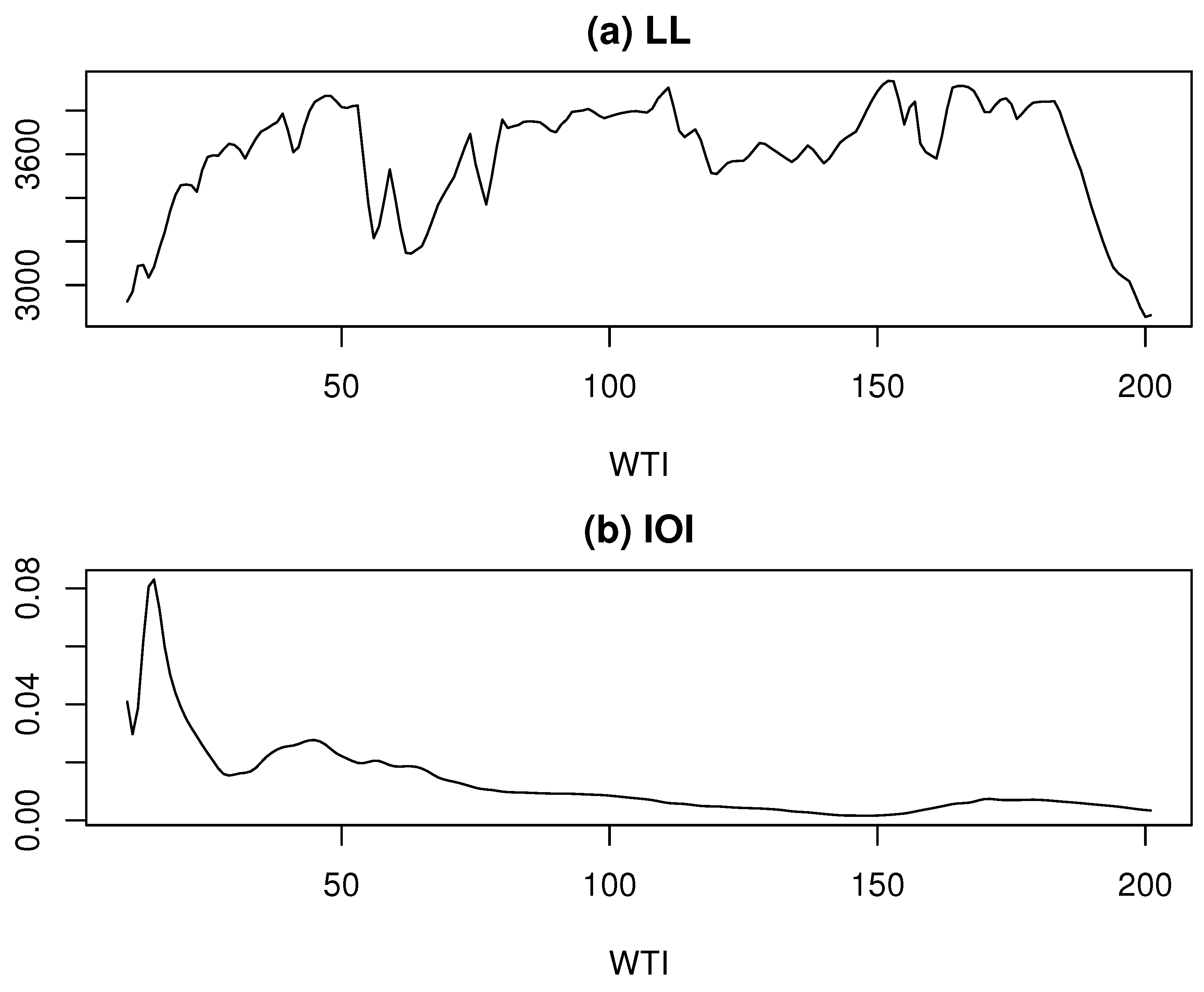
Figure 3.
Log-likelihood and IOI vs. k for the second component decomposition
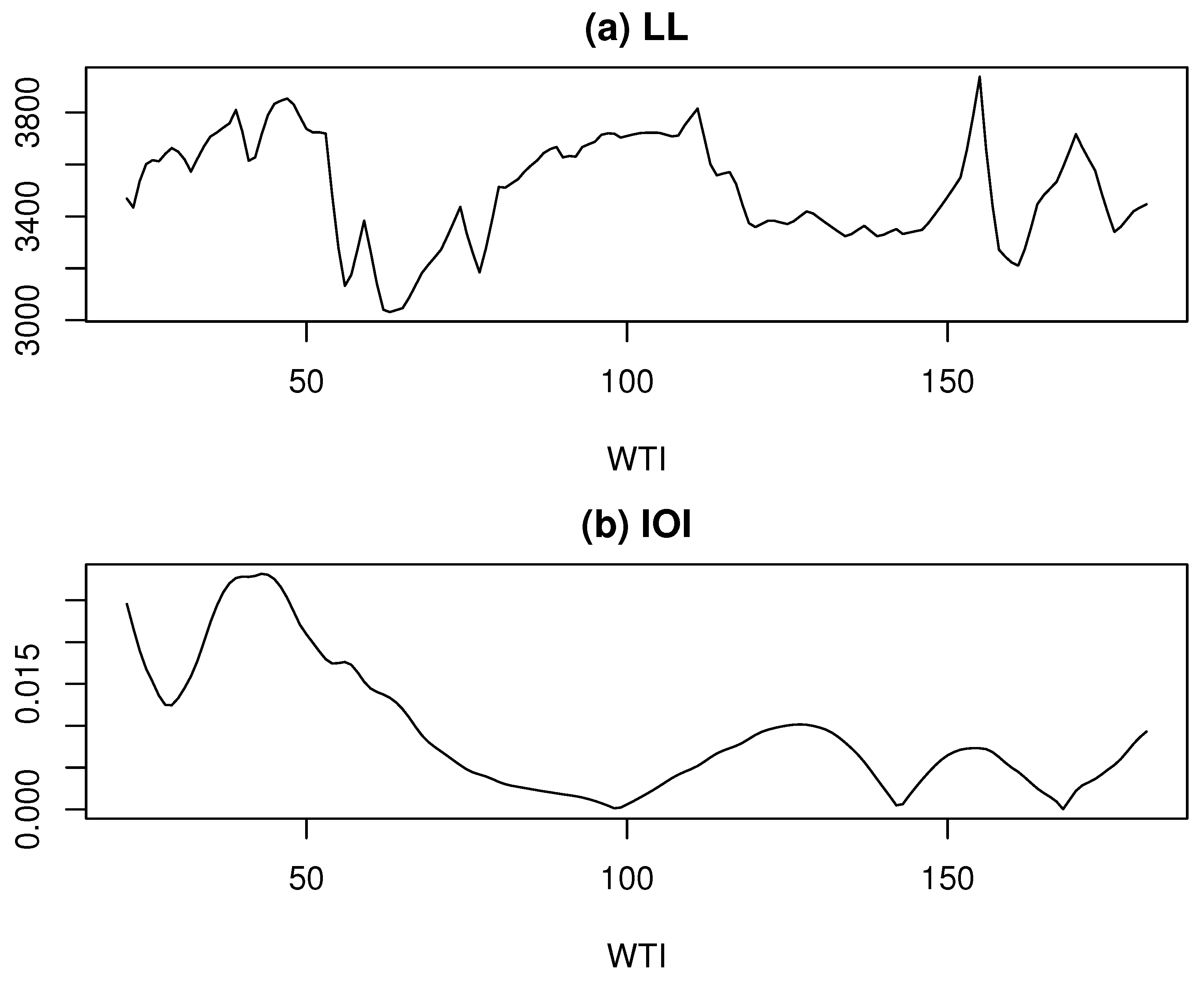
Figure 4.
Results of the second component decomposition
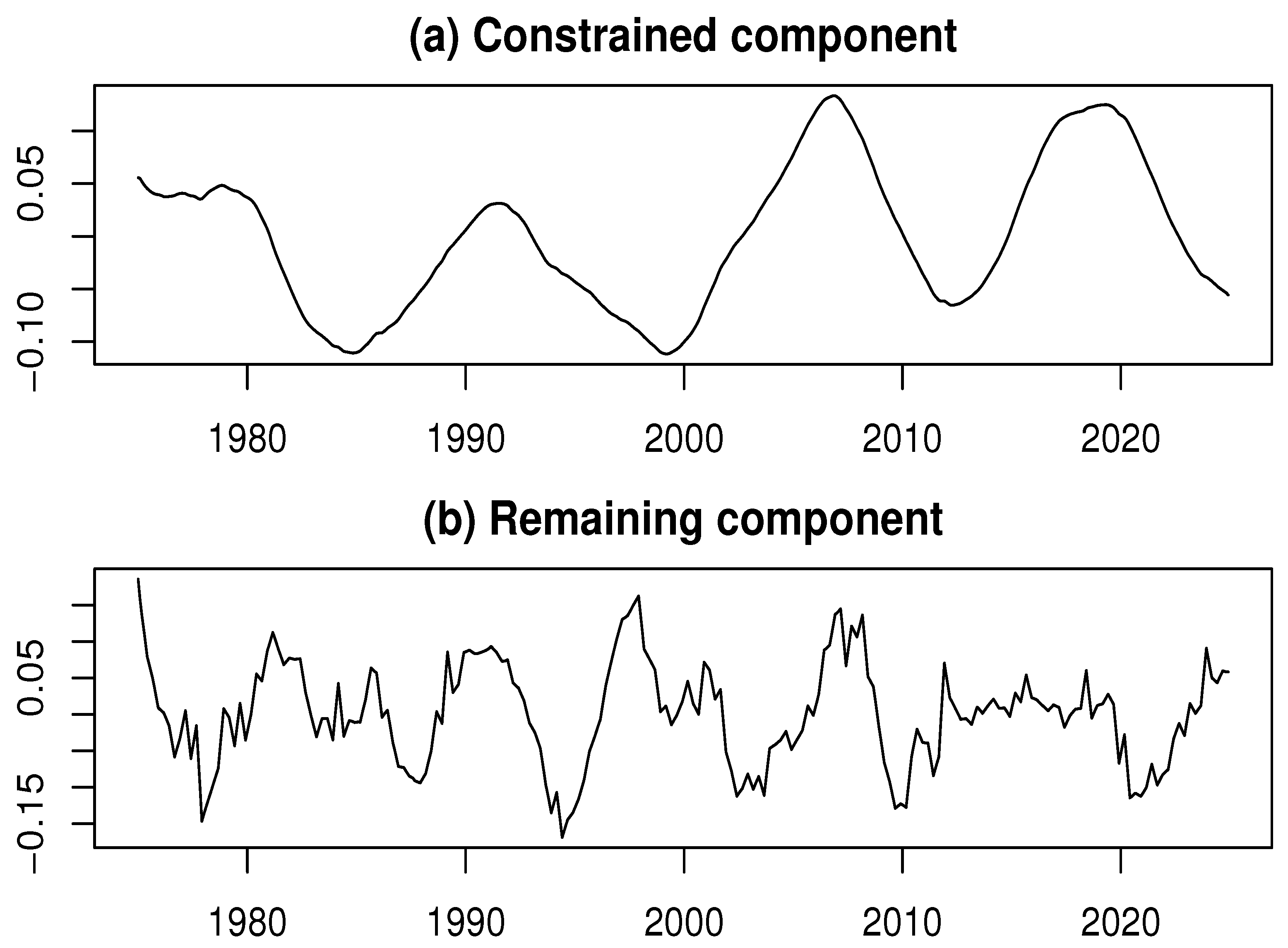
Figure 5.
Log-likelihood and IOI vs. k for the log-SAIIP time series
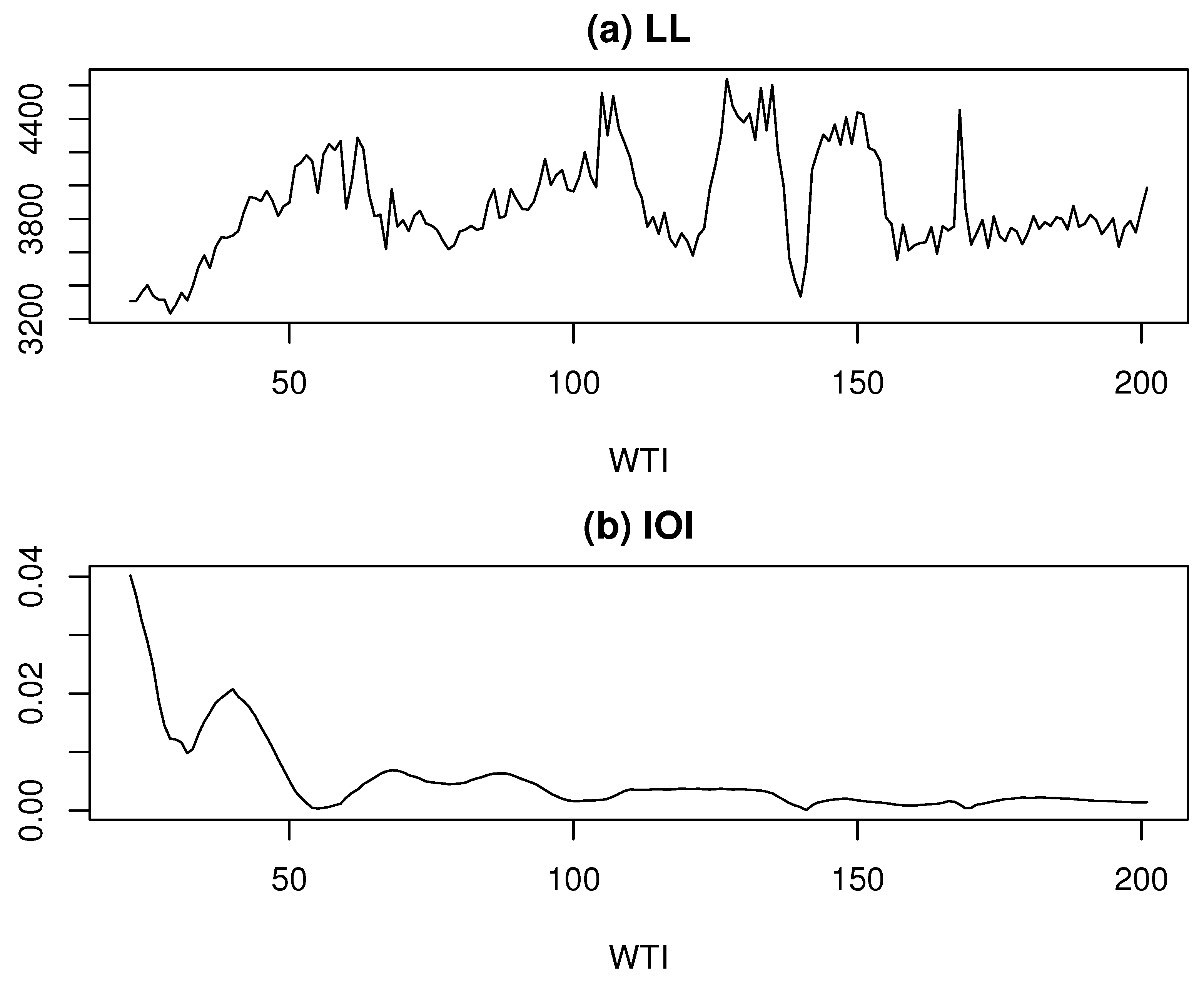
Figure 7.
Final results of decomposition for the log-SAIIP time series
Disclaimer/Publisher’s Note: The statements, opinions and data contained in all publications are solely those of the individual author(s) and contributor(s) and not of MDPI and/or the editor(s). MDPI and/or the editor(s) disclaim responsibility for any injury to people or property resulting from any ideas, methods, instructions or products referred to in the content. |
© 2025 by the authors. Licensee MDPI, Basel, Switzerland. This article is an open access article distributed under the terms and conditions of the Creative Commons Attribution (CC BY) license (http://creativecommons.org/licenses/by/4.0/).
Copyright: This open access article is published under a Creative Commons CC BY 4.0 license, which permit the free download, distribution, and reuse, provided that the author and preprint are cited in any reuse.


