Submitted:
01 May 2025
Posted:
08 May 2025
You are already at the latest version
Abstract
Nowadays Automated Teller Machines (ATMs) are one of the main cash circulation sources in societies. Banks and their clients depend heavily on their availability and their ability to consistently serve client requests. In order to achieve that high availability, banks are trying to optimize their ATM resupply planning in order to ensure client satisfaction while minimizing their own costs and the amount of capital that is idle inside the ATMs. The solution proposed in this paper is trying to find the most fitting algorithms in order to predict the optimal time that an ATM should be resupplied using machine learning techniques. The algorithms take into consideration historical data and external data that may affect the resupply process or the client activity per ATM, such as holidays or street events near the ATM. The results are being used by a route optimization algorithm in order to find the optimal supply planning, minimizing costs and energy consumption.
Keywords:
machine learning
; smart city
; multi-objective optimization
; route optimization
; deep learning
1. Introduction
Modern banking is highly dependent on automation, both on software and hardware level. Automated Teller Machines (ATMs) are so integrated into our everyday lives that we are taking them for granted. The fact is that ATMs are becoming more and more widespread as the banks expand their networks and due to the higher number of machines and the distance between them, managing and supplying them becomes more and more costly. And the demand for constant maintenance and resupply is forcing the banks to assume these costs in order to preserve the client satisfaction that show little tolerance to ATM denials of service.
Due to the vastness of modern day ATM networks, the generated monitoring data are becoming so large and complex that human employees have a hard time making real time decisions and judgment calls about maintenance and supply tasks. This is an issue that can be tackled using machine learning and deep learning, by training a set of models that can predict the maintenance or resupply need of ATMs before that arises. This predictive mechanism has a dual mission, it needs to balance its predictions between ensuring high availability and minimizing the cash tied to the ATMs, since these cash resources are being withheld by the machines and unusable by the banks as long as they remain in them.
The proposed solution that is presented into the present work is examining a set of classical machine learning algorithms and a set of configurations for a deep learning algorithm. The models created using all these algorithms are compared based on their accuracy and stability in order to identify the best configuration that solves the presented problem. The results show that classical machine learning algorithms are pretty powerful, managing to solve the problem with high accuracy, while deep learning also shows some promising results but with a number of consideration that need to be tackled.
The rest of the paper is structured as follows. Section 2.1 presents an overview of the state of the art and related works relevant to the problem presented. Section 2.2 presents the datasets used during the experimental process as well as a set of statistical and preprocessing tasks performed on the datasets. Section 2.4 provides a detailed description of the implemented platform, its capabilities, limitations and specifications. Section 3 presents the results of the experiments and evaluation conducted and finally Section 4 presents the discussion and future work derived from the evaluation.
2. Materials and Methods
2.1. Related Work
A number of preprocessing and transformation works that make machine learning models more efficient in training were identified during the literature survey on analyses and prediction models of similar characteristics. Specifically, we observe that the majority of researchers working on forecasting cash availability or demand at ATMs model the problem as a time series analysis problem [1,2,3,4]. On the other hand, there are some examples that analyze data as a series of independent observations using regression techniques [5,6,7].
Classical, or “traditional” as they are commonly referred to in the literature, machine learning algorithms include algorithms that are based either on creating functions or tree structures. The first category attempts to describe the relationship between training features and the target variable using a function or equation. The second category tackles the same objective creating tree structures, based on specific branching criteria. In algorithms that use mathematical functions each feature is associated with a coefficient. After that, all features along with their coefficients are merged into a single function that uses the feature values as input and outputs the predicted target variable. Algorithms based on tree structures pre-define a set of branching criteria that helps them split the dataset records into branches. These criteria can be functions or thresholds or a combination of them. Each leaf of the tree leads to a specific value or a range of values after a number of splits and tree levels. This creates a path inside the created tree for each vector representing a dataset record. The path leads to the leaf containing the predicted value of the tree.
The Linear Regression (LR) algorithm is one of the most basic and simple algorithms based on functions, being the basis for most of the function based algorithms presented in this section. Its main purpose is to create a linear function consisting of the pre-defined training features and a coefficient for each feature. This function aims to make predictions for the pre-defined target variable. LR always produces a straight line that passes as closely as possible to the training data points, traditionally using the least-squares metric to minimize the error. Naturally, since it is a simple algorithm, it is the fastest and lightest, but it does not produce reliable predictions when the target variable does not have a linear relationship with the features [8].
The Orthogonal Matching Pursuit (OMP) algorithm is a “greedy” algorithm primarily used with sparse data. Its goal is to create a linear function that relates a number of features to the target variable by using a set of coefficients applied to the features. In each iteration of the algorithm, one of the features is chosen based on its degree of correlation with the target variable, and a coefficient is chosen using the least-squares technique. This process continues until each feature is assigned an optimal coefficient, or the accuracy of the predictions does not improve based on the least-squares metric. This algorithm is quite fast and does not require significant computational power, but it is vulnerable to non-homogeneous or noisy data [9].
The Bayesian Ridge (BR) algorithm is also a linear correlation algorithm creating a linear function. Unlike OMP, Bayesian Ridge implements Bayesian techniques derived from the domain of statistics. This algorithm assigns a set of randomized initial coefficients to the features using a Gaussian distribution. Then it attempts to reduce the error in each iteration through Bayesian techniques, producing a different distribution for the feature coefficients. This algorithm is efficient with data sets that have many features and few samples but requires more computational power and it is having difficulties handling data that does not follow common statistical distributions like the Gaussian distribution [10].
The Stochastic Gradient Descent (SGD) Regressor is also a linear regression algorithm that incorporates the SGD methodology to minimize its error during training. It is a fast and light algorithm, as it does not use the entire data set for training. Instead, it uses a small subset of data in each iteration. In more detail, it starts with random coefficients for the features and then tests its deviation from the actual target values, called error, on a small subset of the training data. In each iteration, it changes the coefficients to reduce the error, each time testing a different subset. It is a fast algorithm that easily finds high accuracy solutions, but it is vulnerable to local optima and noisy data [11].
Lasso Least Angle Regression (Lasso-LARS) is an algorithm that combines Least Angle Regression (LARS) and Least Absolute Shrinkage and Selection Operator (LASSO). LARS is an algorithm that works similarly to OMP, building a set of features and coefficients in each iteration that affects the target variable, selecting these features and corresponding coefficients one by one. LASSO improves LARS by setting threshold criteria that reject some features, setting their coefficients to 0. This means that Lasso-LARS is a fast algorithm that creates sparse models with few features. The drawback is that it requires data sets with multiple features to perform this selection. If the data has few features, important ones may be discarded [12].
The Decision Tree Regressor (DRT) is an algorithm based on tree structures. As mentioned, the goal of these algorithms is to create a tree structure where each node is a split condition based on the features and their association with the target variable. Each leaf of the tree has an estimated value for the target variable. In DRT each split is based on a cost function value, typically the mean squared error (MSE) or the mean absolute error (MAE). These trees do not assume a linear relationship between features, nor do they require numeric features, making them affective on heterogeneous training data sets. Their main drawback is that they can easily over-fit the training data and may fail to generalize to previously unseen data [13].
Deep learning is a branch of machine learning based on multi-layer neural networks, with many hidden layers between input and output. Neural networks are networks composed of artificial neurons, called perceptrons, which decide whether to activate or not based on a function applied to the input features. Each neuron, if activated, sends the transformed input features to the neurons in the next layer. Thus, a complex network capable of combining multiple functions, coefficients, and threshold values is formed, aiming to perform a prediction for the target variable. These networks, in their simplest form, are called deep neural networks (DNN) and have existed for several decades [14], but they have only recently become widely used due to advances in available computational power and RAM expansion [15]. Another achievement that has helped significantly is the introduction of graphics cards (GPUs) in model training, as GPUs can perform parallel tasks much faster than traditional processors, improving training times even with large data sets. In Figure 1, we see a graphical representation of such a network with 2 hidden layers. In its traditional form, information flows from left to right (feed-forward network), but in more modern networks, the flow direction can change.
Recurrent neural networks (RNNs) are an evolution of classic DNNs. The main difference is that information can flow backward, allowing neurons that were not activated to have a second chance at activation. This capability makes them more efficient with data that are defined by a specific time sequence, such as time series data, speech, natural language, or video [16]. The directed cycles created by the flow of information allow these networks to leverage features from previous time points, learning cause-and-effect relationships between past feature values. Their drawback is that due to these cycles, RNNs suffer from the vanishing gradient problem, which leads to some neurons being permanently deactivated due to the gradual degradation of their function coefficients. To tackle this issue a set of improvements on the classic RNNs were developed.
One of the most popular RNN improvements is contained in the Long Short-Term Memory (LSTM) networks [17]. Their purpose is to avoid the vanishing gradients problem in classical RNNs, allowing network training with data over a longer time frame, revealing temporal correlations and patterns that are not visible in shorter time windows. This improvement essentially groups neurons into cells that can learn, forget, and forward information. The ability to learn and selectively forget better regulates data flow and learning impact within the network, making LSTMs highly effective with complex data patterns. However, LSTMs are more resource demanding than RNNs, requiring more resources during their training, especially for large data sets. They are also vulnerable to over-fitting, often creating models that are unable to handle previously unknown data efficiently.
2.2. Datasets
The models are using a database that pools data belonging to two distinct types: a) ATM supply data and b) ATM fault data. These two types of data are merged into a single database that contains both supply and fault data for each of the ATMs examined. The database contains 40016 records that span the year 2023 and 6123 records for the first two months of 2024. The separation per year is necessary since the data of year 2023 are used as training data for the models, while the data from year 2024 are used as test and evaluation data for the validation of the models’ performance. Each distinct record of the database has the following fields:
- ATM identification code.
- Location of the ATM.
- Company responsible for the supply of the ATM.
- Type of event.
- Date of event.
A timeseries, according to the science of mathematics, is a series of data that are placed into chronological order. In machine learning this definition is even more limiting, adding the limitation that that these data points must have a causality relationship between them, especially data points that are temporal neighbors. Timeseries are a classic example of data used in machine learning training due to the easy and intuitive pattern extraction tied with their nature. Moreover, they are making the stationary analysis process easier, revealing if the data contain a pattern that repeats itself over regular time intervals. These patters are extremely useful in machine learning model training as they enhance the predictive accuracy of the model. This kind of data needs certain steps of preprocessing so that they are reshaped into a form usable by the machine learning models. In more detail, they need to be cleansed from redundant or erroneous information and to be analyzed in order to identify features that can be extracted from them, features that are directly related to the prediction target by a causal relation. Moreover, missing data should be handled by data reconstruction techniques. These preprocessing steps will be analyzed into more detail in Section 2.2.2.
On the other hand, independent data are also comprised of data points that are placed in a chronological order, like the timeseries, but these data points do not necessarily have strict time intervals between them, have no missing points between them or even have a strict causality relationship between two temporal neighboring points. Algorithms being trained on these datasets do not take for granted that there is a causal relationship tied to the temporal placement of the data points, instead they are looking for patterns that reveal hidden correlations between the extracted features and the current value of the target variable. In other words, the main aim of the machine learning algorithms is to create a function that takes as input a vector of feature values and give a predicted value for the target variable as an output. As a result, these datasets demand a different preprocessing methodology and reformatting prior to the training process of the machine learning algorithms that will be presented in detail in Section 2.2.2.
2.2.1. Statistical Analysis
As a first step to evaluate the uniformity of the data per ATM a histogram was created, visualizing the total number of ATM supply records for each machine. The histogram is presented in Figure 2. By studying it we can see that the vast majority of the ATM have less than 80 distinct records with most ATMs (123 machines) having 31-41 records. Moreover, we can see that just 13 ATMs have over 130 records. This analysis provides a first outlook of the data and the thresholds we can set about the number of records for a predictive model to be considered adequately trained. As will be presented shortly, the threshold we selected during the data cleansing process was 20 records, meaning that most of the ATMs that belong in the 1-11 bucket of the histogram will be cleansed out of the useful dataset. Some of the ATMs will be rescued due to the data filling that will be performed and described in Section 2.2.2.
Figure 3 presents a histogram depicting the average distance in days between two neighboring events per ATM. This histogram shows that the vast majority of ATMs are supplied once every 1 to 4 days, with only 14 machines having average interval of more than 6 days. This analysis reveals the time interval that the predictive models should target. In most cases, the prediction interval should be set to just 1 day, meaning the next day. As an extra mile, to cover even more cases, the models should be able to predict the need for supply up to 3 days in the future.
Figure 4 presents the last histogram for this analysis, depicting the maximum time interval between supply events per ATM. The histogram reveals that almost half of the ATMs have maximum time interval of only one day, meaning that they are being supplied each day without exceptions. On the other hand, the dataset contains 370 ATMs that are supplied in rare occasions, even once per 24 days, almost once per month. According to the histogram presented in Figure 3 this is not the usual case, even for these machines, but they can still remain without a need for supply for many days under specific circumstances that are to be revealed by the machine learning models.
The stationary data analysis examines if the values of the target variable have some form of repetition over the course of time. It is a classic analysis that is executed in problems of this category [18,19,20]. The analysis of our target variable, which is the “value-t” variable describing the percentage of filled capacity of an ATM at the time “t”, gave an average stationary score of 0,0018. This score means that the timeseries presents a high ration of stationarity at a weekly level, as it is a great deal smaller than the 0,005 threshold that the literature defines as the validity threshold of the stationary analysis. This means that the choice of this specific variable as the prediction target is completely justified and a machine learning model would be successfully trained on the available data with high confidence rates.
2.2.2. Preprocessing
As the first step of preprocessing the dataset was cleansed in order to remove records that are not useful to the models or can even confuse it during the training process. Two distinct categories of such records were identified in the dataset:
- Records that do not have enough width. These include records for an ATM that fail to cover at least 70% of the year in time interval between the first and last supply event.
- Records that do not have enough volume. These include records for an ATM that has less than 50 distinct records in the dataset.
Of the 863 ATMs in the complete dataset, 202 did not have more than 20 records and were therefore considered unusable by the models. Of the 661 ATMs that remained, 18 did not cover 70% of the year between their first and last record, so they were also considered unusable, leaving 643 machines. The test data provided by the use case owner covers the first two months of 2024 and includes records for only 24 ATMs out of these 643. Thus, 24 different models were trained and evaluated, one for each ATM that remained in the dataset.
The next step was the enrichment of the records with external or secondary, derived data, creating more columns. These extra columns will be used during the training of the models in order to uncover more hidden patterns that affect the usage demand of ATMs. In detail, the columns that were created are the following:
- Day of the week: Monday up to Sunday.
- Workday: true or false.
- Holiday: true or false.
- Capacity difference from previous day: real number from -1.0 to 1.0.
- Days to next supply: natural number.
The next step of the preprocessing is the transformation of the data in a timeseries format, so that they can be used by the prediction model. Timeseries data, or just timeseries, are datasets that follow a strict temporal order. In addition, the values that are observed in each time step are dependent in some manner to the values observed in previous time steps. In order to transform the the dataset into a timeseries we just have to order the data points into chronological order, according to the record timestamps and then fill the missing time steps, creating steady time intervals between the data points. This data filling process was conducted using a simple linear function, making the assumption that the percentage of filled capacity of an ATM follows a linear degradation through time. For example, using Function 1 where is the capacity at time step t and is the day at time step t, if an ATM is observed at 100% capacity on day 1 and then at 25% capacity on day 4 we assume that it has a reduction of per day. So, at day 2 it would be at 75%, at day 3 it would be at 50% and on day 4 it would be at 25% as observed.
The last step of the preprocessing is the transformation of the dataset into a form that can be used for deep learning training. This transformation creates a set of columns that correlate the data points of previous time steps to the current value of the prediction target. Which means that if the target is to predict the capacity percentage of the ATM for the next day and we want to only consider the data of the current day, we would have a dataset consisting of the data points presented in Table 1. In detail, the data presented are translated by one day in the past, at time step while the prediction target, which is the remains at time step t, containing the capacity value of the next day. During the experimental process presented in Section 3, this temporal translation was conducted for greater time intervals, up to seven days in the past.
As training features for the deep learning model a subset of these columns was selected, based on our experience, practical experiments and the relevant literature. In order for a column to be selected as a feature it needed to present the following characteristics:
- Be balanced, without having unexplained and steep fluctuations.
- Be correlated to the target variable, meaning that changes in their value affect the value of the target variable either directly or indirectly.
- Do not contain missing or erroneous data.
- Be in or can be converted to numerical form.
- Be independent between them, meaning that they are not directly correlated, since correlated values can be omitted to simplify the model, they do not offer new information to the model.
Having these criteria in mind the selected variable was while the selected features were the following:
A set of alternative features tests were also conducted separating the column into seven distinct boolean features according to the relevant literature [4] but it did not have any important effects on the evaluation of the models.
2.3. Problem Formulation
Since the posed problem is a complex one, involving the prediction of ATM cash availability and the optimization of supply routing, we deem it necessary to clearly define the problem and its parameters in a formal fashion. Let be the set of N ATMs that form our ATM network. Each ATM has a cash availability function which defines its cash availability rate over time.
Moreover, there is a set of supply vehicles , with each vehicle having a capacity and operating within a predefined service window, forming the basis of a Capacitated Vehicle Routing Problem (CVRP). In our case, since we do not have any data regarding the capacity or the number of the vehicles due to security reasons, the set of supply vehicles can be considered large enough to cover each ATM and their capacity can be considered large enough to carry the maximum capacity of the ATMs each vehicle is responsible for. Under these assumptions, the CVRP can be simplified into a multiple Traveling Salesman Problem (mTSP), where each vehicle is a traveling salesman trying to cooperatively visit each ATM in the network.
The challenge posed is to determine the optimal supply plan, achieving three objectives:
- Cash shortages are minimized allowing ATMs to serve client requests.
- Operational costs are minimized ensuring minimized costs for the National Bank of Greece during supply actions.
- Total idle capital across the ATM network is minimized, avoiding excessive cash storage and bank liquidity problems.
2.3.1. Available Cash Forecasting
In order to create the available cash prediction model we need to define the function for each ATM. This function should take the prespecified feature set as an input and provide an estimate of the available cash at time t as an output. A critical cash threshold is also defined for each ATM, setting the safety threshold under which cash shortages are commonly occurring. The function, based on the dataset described in Section 2.2, should have the following form:
where:
- is the day of the week at time t
- is the day of the month at time t
- is the month at time t
- is 1 if the day at time t is a workday or 0 if not
- is 1 if the day at time t is a holiday or 0 if not
- is the value of filled capacity for the ATM at time
- is the prediction error for ATM and time t
- is the prediction model function as trained using a selected algorithm
2.3.2. Supply Plan Optimization
Forming the mTSP definition requires that the ATM network is formally defined as a graph where is the set of nodes and E is the set of edges that represent roads from one node to another. The set of nodes N contains each ATM that needs to be supplied at time t and a central node 0 which represents the supply station from where the vehicles load their cash and start their route. An ATM is in need of supply if and only if for time t. Each edge is accompanied with a weight which represents the cost of using this path, in our case this equals to the physical distance of the path. Having that in mind, we define a set of variables which becomes 1 if the vehicle uses the edge or 0 if it does not. It is obvious that for each time t a new graph G is created, representing the state of the network at time t.
Optimizing the supply plan requires the definition of three functions that form the multi-objective optimization goal. The functions are defined as follows:
- Minimization of operation costs:
- Minimization of cash shortages:
- Minimization of idle capital:
- Each ATM is visited exactly once:
- Each vehicle starts at the supply station:
- Forcing single continuous routes for each vehicle, with being the position of ATM in the route:
Gathering these objective functions we can create a multi-objective optimization function as follows:
where , , are the weights assigned to each objective function, representing the importance of the function to the multi-objective optimization problem.
2.4. Experimental Setup
The implementation of the models is quite complex due to the multiple data format options and algorithms forming the exploration space. Thus, it was decided to design and implement a system of three distinct components that are interconnected and assist in the process of data extraction, storage, analysis and preprocessing, in the configuration, training and evaluation of classical machine learning models based on regression and mathematical models but also in the configuration, training and evaluation of machine learning models based on deep learning techniques. A high level architecture of the proposed system is depicted in Figure 5. The system consists of the following components:
- Data Manager: the component responsible for data extraction, storage, analysis and preprocessing.
- Machine Learning: the component responsible for configuration, training and evaluation of the classical machine learning models.
- Deep Learning: the component responsible for configuration, training and evaluation of the deep learning models.
In detail, Data Manager aims to provide unified management of the entire course of data from data collection to machine learning model training. It also has a number of functions that help in storing and analyzing the results of model evaluation. It starts with data collection by receiving the data in the format provided by the National Bank of Greece (NBG). During the experiments in the presented work, the data were provided in CSV and EXCEL file formats. These files were read by the Data Manager, transformed into easily manageable data formats, such as Python dictionaries and Pandas DataFrames, and then stored in a local NoSQL database (MongoDB) in JSON format.
Data Manager, in addition to extracting and storing analyzed data, also provides data analysis mechanisms, able to perform a set of a-priori analyses presented in Section 2.2.1. These tools consist of mathematical functions that aim to extract statistical information about the data in order to assess their quality and determine the necessary preprocessing steps and configuration. Finally, Data Manager introduces data preprocessing methods utilizing the knowledge provided by the data analysis, as well as the literature, in order to clean, fill and transform the data in such a way as to enhance the training of machine learning models. In addition, during the preprocessing phase, some secondary data are also produced that are later selected as features for training the models.
Machine learning implements the next step, providing various classical machine learning algorithms that mainly try to create mathematical models and functions that connect the training data points to the respective values of the target variable. The models that have been tested and implemented on this platform are those provided by the Scikit-learn package of Python and are presented in detail in Section 2.1. Specifically, the Machine Learning platform provides models that are created with the following algorithms and methodologies:
- Orthogonal Matching Pursuit (OMP)
- Bayesian Ridge
- Stochastic Gradient Descent (SGD) Regressor
- Lasso Least Angle Regression (Lasso-LARS)
- Linear Regression
- Decision Tree Regressor
To train one of these algorithms, creating the prediction model, we need to use the preprocessed data produced by the Data Manager as input, or training, data and select the target variable (or column) of the model and the features to be used for training the models. These features constitute a subset of the available columns of the dataset. The feature selection was done based on the evaluation and after many successive experiments with feature swaps and parameter optimizations.
The Deep Learning platform is the third and final platform of the proposed system. It implements machine learning models based on deep learning, creating complex and multi-layered networks of artificial neurons. During the experiments conducted in the context of the presented work, the platform implements the Long Short Term Memory (LSTM) algorithm which in practice creates a Recurrent Neural Network, a subcategory of deep learning networks that has proven to be quite efficient in learning time series. As we will see in Section 3, the evaluation of the model shows a promising accuracy and general performance for the generated model.
The prediction target of the model was the percentage of filled capacity per ATM, denoted as in function 2. By predicting this value, we can accurately calculate the day when the machine will need to be supplied in order to avoid the situation where the ATM does not have enough money to serve the demand, which is the main goal of objective function 4. During the evaluation, the available preprocessed data were grouped by ATM, transferring the prediction problem to an ATM level. This means that the demand forecast for each individual ATM is now a separate problem, independent of the others, and therefore requires the training of a separate machine learning model.
3. Results
3.1. Classical Machine Learning Models
These 24 models were trained and evaluated 6 times, one for each algorithm in the exploration list. The results of the evaluations are depicted in Figure 6. As the evaluation metric we selected the Median Absolute Error (MAE), which is mentioned as the most fitting metric for this kind of experiments in the relevant literature [1,2,6]. The most effective algorithms based on MAE were SVC, Random Forest Regressor and Bayesian Ridge. In the chart presented in Figure 6 we can see three metrics for each algorithm: a) minimum MAE, b) average MAE and c) maximum MAE. These metrics provide a good estimation of the prediction error that is present in function 2.
Decision Tree Regressor manages to minimize all three metrics compared to the other algorithms, proving itself as the most accurate. Table 2 presents a more detailed report of the MAE values for each algorithm. In addition to the information presented in Figure 6 we can see that Lasso Lars is the most stable algorithm, having the minimum standard deviation (STD).
3.2. Deep Learning Models
The deep learning models used the same dataset of 24 ATMs that was used for the models developed using classical machine learning algorithms. This led to the creation of 24 new models, one for each ATM, using the Long Short Term Memory (LSTM) algorithm. This algorithm allows us to define various time windows that it can take into consideration during its training and inference phases. This ability led to the training of six variations of the algorithm, having time windows of size 1 up to 6 days in the past, the results of which are presented in Figure 7, Figure 8, Figure 9, Figure 10, Figure 11 and Figure 12. The Figures present the evolution of average MAE through the training epochs, or iterations, of the model of a random ATM that was selected for visualization purposes. One epoch, or iteration, consists of a full round of LSTM training, allowing all neurons of the deep neural network to be trained into the values of the presented dataset. One of the conclusions we can extract from the presented Figures is that as the time windows grows larger, the algorithms becomes more erratic, presenting many fluctuations on its accuracy. For example, we can see in Figure 7 that the lines are pretty stable, following a convergence course after epoch 80. On the other hand, Figure 8 shows that the line has a more “wavy” form, presenting greater instability on its accuracy. This observation has two main applications: a) it shows that predicting the capacity of an ATM for the next day is more stable and accurate than predicting its capacity for next 6 days and b) it shows that having the daily data as input for the next inference is more effective that having data from a wider historical window.
Table 3 presents a detailed analysis of the MAE metrics for each time window examined. The values are normalized in the 0 - 100 range for easier comparison. A first observation is that as the time window grows, the model becomes more accurate, reducing the error margin. This is caused by the fact that as the time window grows, the model receives more data, enhancing its opportinities of uncovering hidden patterns and learning the causality relationships between the features and the target variable, especially if we consider that the stationary analysis presented in Section 2.2.1 reveals a pattern repetition in weekly intervals. This may appear to conflict the instability we observed in Figure 7, Figure 8, Figure 9, Figure 10, Figure 11 and Figure 12 but it does not because the instability we observed is during the training of the model, making it more erratic during training, the accuracy we are observing here is during evaluation, making it more accurate after the training. The Figures show us how sensitive the model is to feature variations while Table 3 shows us how accurate its predictions are.
3.3. Use Case Evaluation
For the evaluation of the real world application tied to the models an experiment using the test data was conducted. The scenario of this experiment is that NBG personnel are using the models in order to decide the list of ATMs that need supply the next day. For this test we used the test and evaluation dataset described in the previous sections. In detail, the data used spanned the first two months of 2024, having 24 different ATMs. Regarding the model used, we decided to use the most accurate model identified during the tests presented in Section 3.1 and Section 3.2, meaning the Decision Tree Regressor. Figure 13 presents a prediction course for the Decision Tree Regressor during the use case evaluation for reference. The dotted line depicts the actual capacity values while the solid line depicts the predicted values.
The results of the evaluation show that there is an average to good performance of the model, caused mainly by the small volume of training data, limiting the training effectiveness of the models. leading to the assumption that as the model is used and more historical data are being collected, the accuracy of the model would become better and better. As success we define the state that the model accurately predicts that an ATM will need supply the following day while as deviation of X days we define the prediction that an ATM will need supply X days later or sooner than the actual need.
During the evaluation we observed an accuracy of about 49% for the next day prediction, about 20% for 1 day deviations, about 15% 2 days deviations and about 25% for more than 2 days deviations. Figure 14 visualized the confusion matrix of the predictions already mentioned for the whole evaluation dataset. The vertical column presents the actual days until the next supply event while the horizontal presents the predicted values. The cells of the matrix contain the number of events that correspond to each row and column of the matrix. We can see that the model is biased into more secure predictions, ensuring that the ATMs have sufficient capacity to serve their clients, providing often 1 or 2 day deviations sooner than the actual supply need. This means that the model achieves the goal of high availability while giving smaller priority to the secondary goal of minimizing the amount of cash being stored in the ATM network.
In parallel to the analysis of the predictive accuracy of the algorithms, a multi-objective optimization evaluation was executed, based on the optimization goals defined in Section 2.3 and, more specifically, the functions 3, 4 and 5. The evaluation was conducted by comparing the values of these functions for the historical data present in our test dataset versus the data that were provided by the predictive and optimization models for each time t. The results show that the value of function 4 () was always at 0, both in the historical and evaluation data, essentially removing it from the multi-objective function. Figure 15 provides a visualization of the comparison for the values of function 5 (). We can see that the proposed platform manages to reduce the total amount of idle capital by about 42.9% when compared to the historical data. In more detail, the average percentage of idle capital capacity per ATM is at 16.54% in the historical data while the cash availability model, using the decision tree regressor, manage to reduce that to 9.44%.
In order to evaluate the effectiveness of the models in minimizing the operation costs of supply plans, according to function 3 (), we measured the maximum percentile of optimal solutions discoverable by each algorithm, for each time t. The algorithms used were three common algorithms in multiple traveling salesman problems, namely ILP, Greedy and Genetic. We observed that the ILP algorithm was providing an optimal solution, placing the value of at the top 0.5% of the possible solution space, when the possible solutions were ranked from minimum to maximum based on the value of . For comparison we also tested the Greedy and Genetic algorithms, in order to provide more lightweight options that allow real time optimizations in contrast to the slow and resource demanding optimizations performed by ILP. The Genetic algorithm achieved scores placed in the top 5% of solutions while the Greedy algorithm was at 16% of the top solutions. By combining these scores into the multi-objective function 9 we get the scores presented in Table 4, setting all three weights , and to 1 for equal objective priority. The table shows that the combination of decision tree regressor and ILP provide the best combination for the platform.
4. Discussion
It is worth mentioning that even though the LSTM model appears to be quite efficient both in prediction accuracy and in stability, with small standard deviation scores, it does not manage to outperform some of the classical machine learning algorithms. Specifically, we observe that the Decision Tree Regressor algorithm is by far the most efficient for this specific dataset as its average error is approximately 6 times smaller than the average error of the LSTM. This may be due to the small number of records that simplifies the problem to a simple linear equation, making the LSTM too complex to solve this problem. If the dataset included several years and additional external factors, perhaps deep learning would give us better solutions but that is not the case here. This hypothesis as well as a larger number of possible deep learning technologies will be examined in the second version of the model, planned as future work. These new data points will provide greater depth and complexity to the patterns that emerge, bringing the model closer to the real world. This additional complexity is expected to reduce the performance of classic machine learning technologies and increase the performance of deep learning models, while taking into account more complex phenomena and currently unexpected deviations.
Author Contributions
All authors contributed equally to the presented work, have read and agreed to the published version of the manuscript.
Funding
This work was supported by the European Union NextGenerationEU Recovery and Resilience Facility programme in the context of the RESEARCH-CREATE-INNOVATE 16971 framework (Project ATMO-MoRe, id: TAEDK-06199)
Data Availability Statement
The data used in the presented research are designated as private and cannot be shared since they concern the operations of the National Bank of Greece.
Conflicts of Interest
The authors declare no conflicts of interest.
References
- Ekinci, Y.; Serban, N.; Duman, E. Optimal ATM replenishment policies under demand uncertainty. Operational Research 2021, 21, 999–1029. [CrossRef]
- Rafi, M.; Wahab, M.T.; Khan, M.B.; Raza, H. ATM cash prediction using time series approach. In Proceedings of the 2020 3rd International Conference on Computing, Mathematics and Engineering Technologies (iCoMET). IEEE, 2020, pp. 1–6.
- Rafi, M.; Wahab, M.T.; Khan, M.B.; Raza, H. Towards optimal ATM cash replenishment using time series analysis. Journal of Intelligent & Fuzzy Systems 2021, 41, 5915–5927. Publisher: IOS Press, . [CrossRef]
- Sarveswararao, V.; Ravi, V.; Vivek, Y. ATM cash demand forecasting in an Indian bank with chaos and hybrid deep learning networks. Expert Systems with Applications 2023, 211, 118645. Publisher: Elsevier.
- Tang, J.; Wang, S.; Bai, T.; Lu, S.; Xiong, J. Intelligent ATM replenishment optimization based on hybrid genetic algorithm. In Proceedings of the 2022 24th International Conference on Advanced Communication Technology (ICACT), 2022, pp. 469–475. ISSN: 1738-9445, . [CrossRef]
- Rajwani, A.; Syed, T.; Khan, B.; Behlim, S. Regression analysis for ATM cash flow prediction. In Proceedings of the 2017 International Conference on Frontiers of Information Technology (FIT). IEEE, 2017, pp. 212–217.
- Joseph, H.R. Combining Traditional Optimization and Modern Machine Learning: A Case in ATM Replenishment Optimization. In Proceedings of the Progress in Industrial Mathematics at ECMI 2014; Russo, G.; Capasso, V.; Nicosia, G.; Romano, V., Eds., Cham, 2016; Mathematics in Industry, pp. 1047–1055.
- James, G.; Witten, D.; Hastie, T.; Tibshirani, R.; Taylor, J. Linear regression. In An introduction to statistical learning: With applications in python; Springer, 2023; pp. 69–134.
- Mallat, S.G.; Zhang, Z. Matching pursuits with time-frequency dictionaries. IEEE Transactions on signal processing 1993, 41, 3397–3415. Publisher: IEEE.
- Bishop, C.M.; Nasrabadi, N.M. Pattern recognition and machine learning; Vol. 4, Springer, 2006.
- Lizhen, W.; Yifan, Z.; Gang, W.; Xiaohong, H. A novel short-term load forecasting method based on mini-batch stochastic gradient descent regression model. Electric Power Systems Research 2022, 211, 108226. Publisher: Elsevier.
- Song, S.; Li, S.; Zhang, T.; Ma, L.; Zhang, L.; Pan, S. Research on time series characteristics of the gas drainage evaluation index based on lasso regression. Scientific Reports 2021, 11, 20593. Publisher: Nature Publishing Group UK London.
- Rady, E.; Fawzy, H.; Fattah, A.M.A. Time series forecasting using tree based methods. J. Stat. Appl. Probab 2021, 10, 229–244.
- Hopfield, J.J. Neural networks and physical systems with emergent collective computational abilities. Proceedings of the National Academy of Sciences 1982, 79, 2554–2558. Publisher: Proceedings of the National Academy of Sciences, . [CrossRef]
- Haykin, S. Neural networks: A comprehensive foundation; Prentice Hall PTR, 1998.
- Zhang, J.; Man, K.F. Time series prediction using RNN in multi-dimension embedding phase space. In Proceedings of the SMC’98 Conference Proceedings. 1998 IEEE International Conference on Systems, Man, and Cybernetics (Cat. No. 98CH36218). IEEE, 1998, Vol. 2, pp. 1868–1873.
- Gers, F.A.; Schmidhuber, J.; Cummins, F. Learning to forget: Continual prediction with LSTM. Neural computation 2000, 12, 2451–2471. Publisher: MIT press.
- Rhif, M.; Ben Abbes, A.; Martinez, B.; Farah, I.R. A deep learning approach for forecasting non-stationary big remote sensing time series. Arabian Journal of Geosciences 2020, 13, 1174. Publisher: Springer.
- Dixit, A.; Jain, S. Effect of stationarity on traditional machine learning models: Time series analysis. In Proceedings of the Proceedings of the 2021 Thirteenth International Conference on Contemporary Computing, 2021, pp. 303–308.
- Schnaubelt, M. A comparison of machine learning model validation schemes for non-stationary time series data. Technical report, FAU Discussion Papers in Economics, 2019.
Figure 1.
Visualization of a neural network.
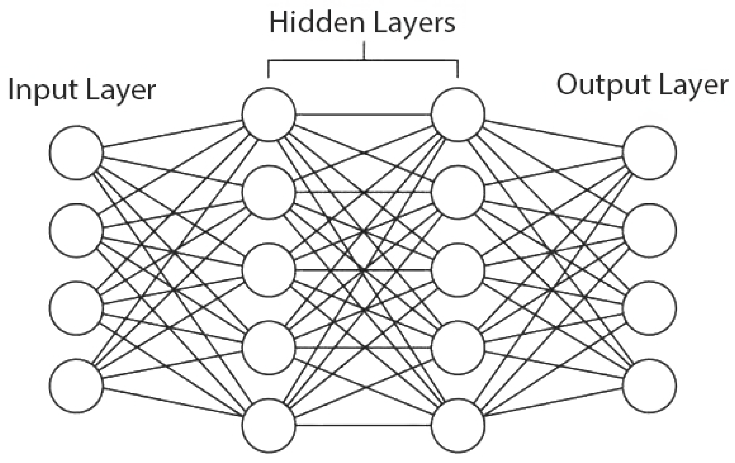
Figure 2.
Histogram of supply data records per ATM.
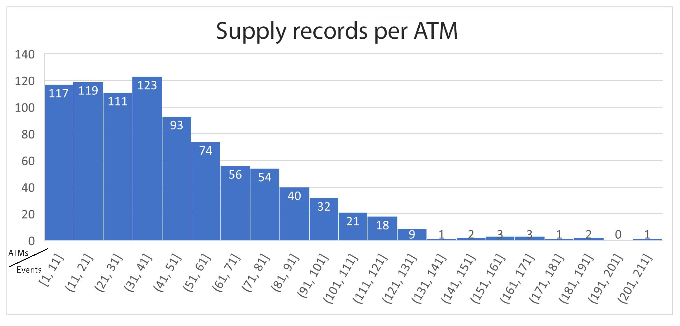
Figure 3.
Average time interval between two supply events in days per ATM.
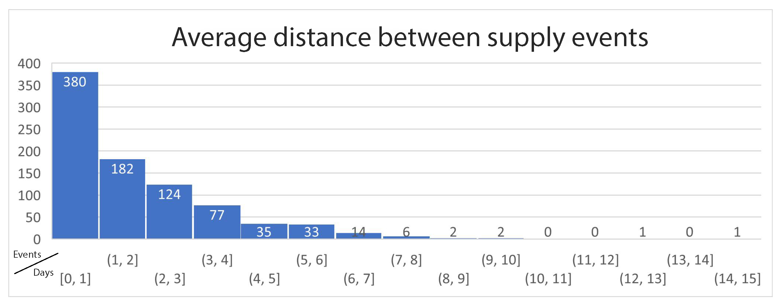
Figure 4.
Maximum time interval between supply events in days per ATM.
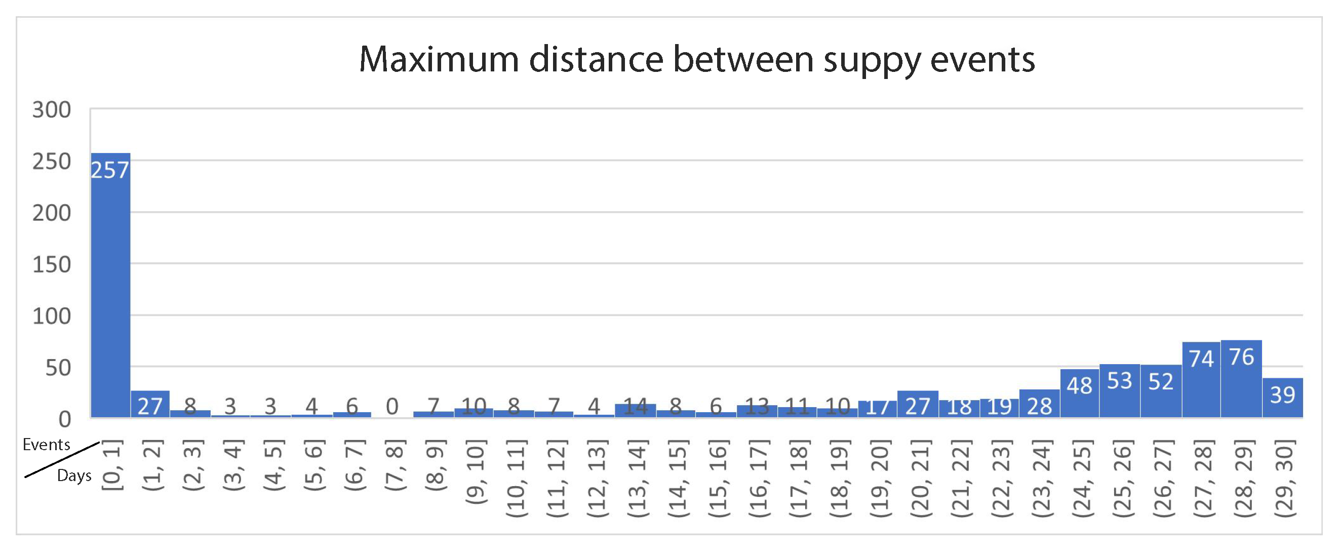
Figure 5.
High level architecture of the proposed machine learning and data management system.
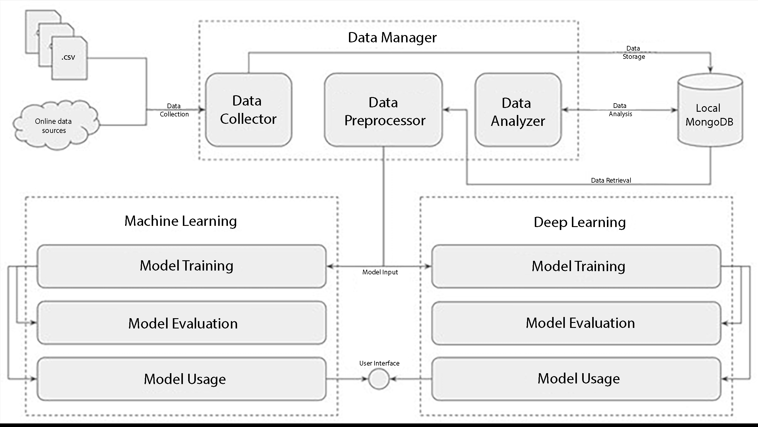
Figure 6.
Comparative analysis of classical machine learning model prediction accuracy.
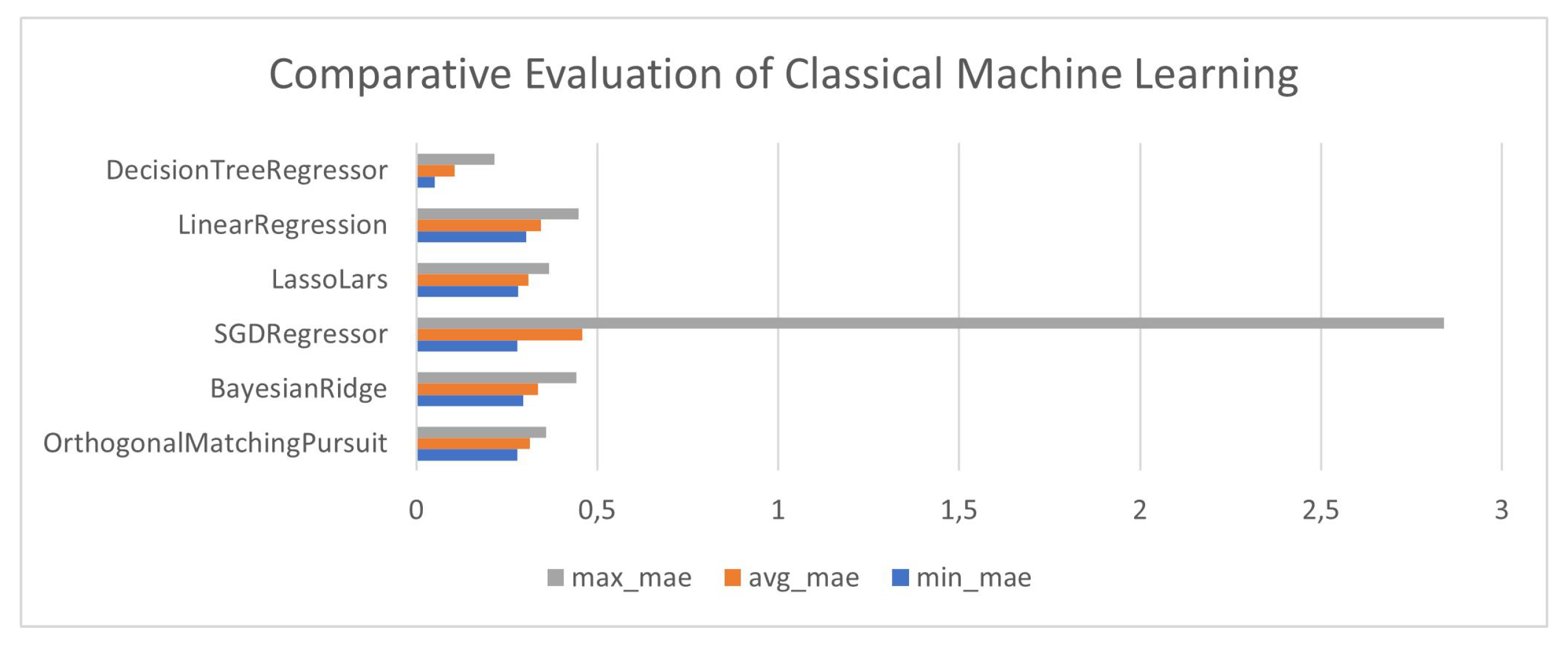
Figure 7.
Error cost evaluation during LSTM training with 1 day window.
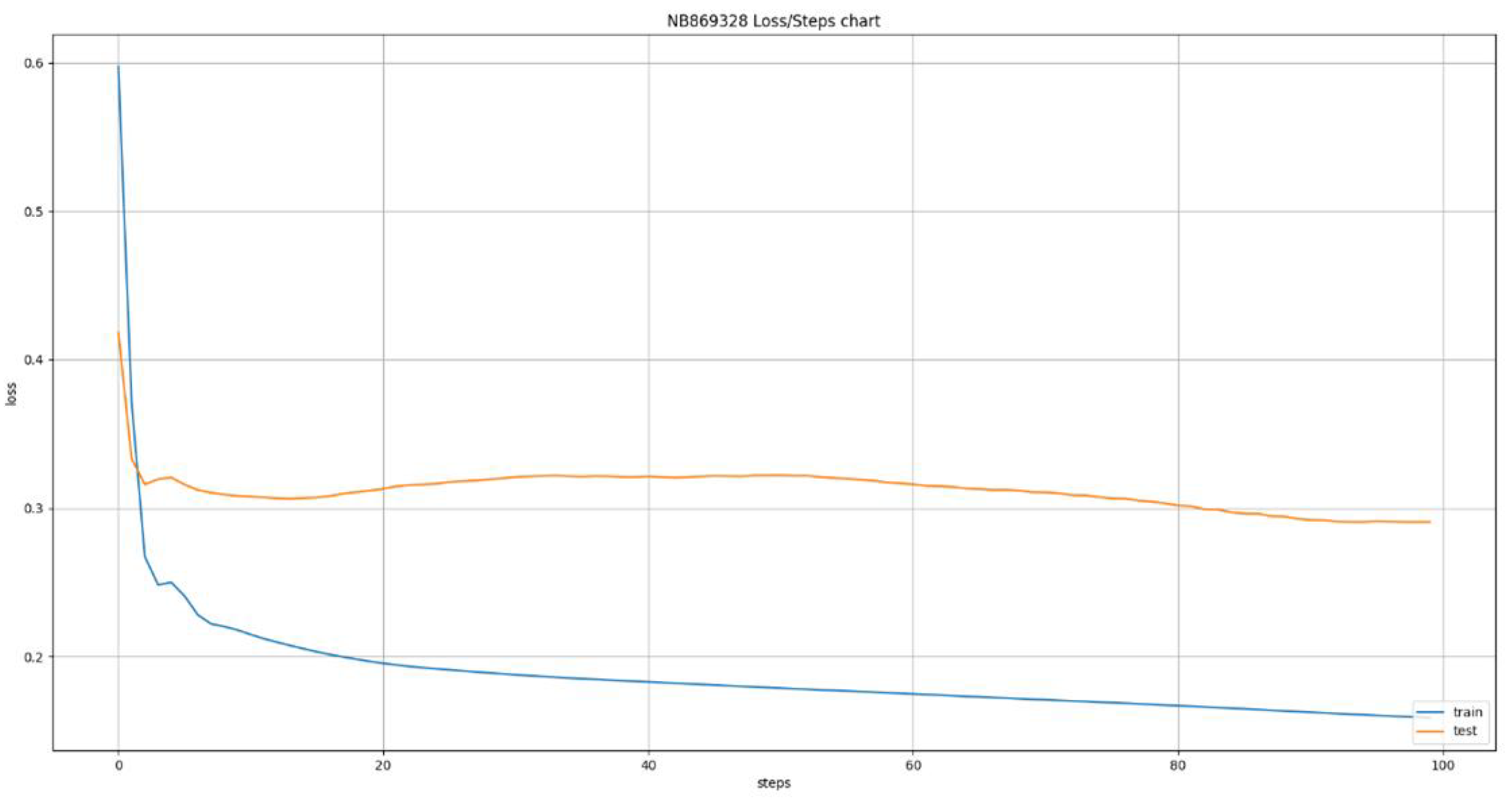
Figure 8.
Error cost evaluation during LSTM training with 2 day window.
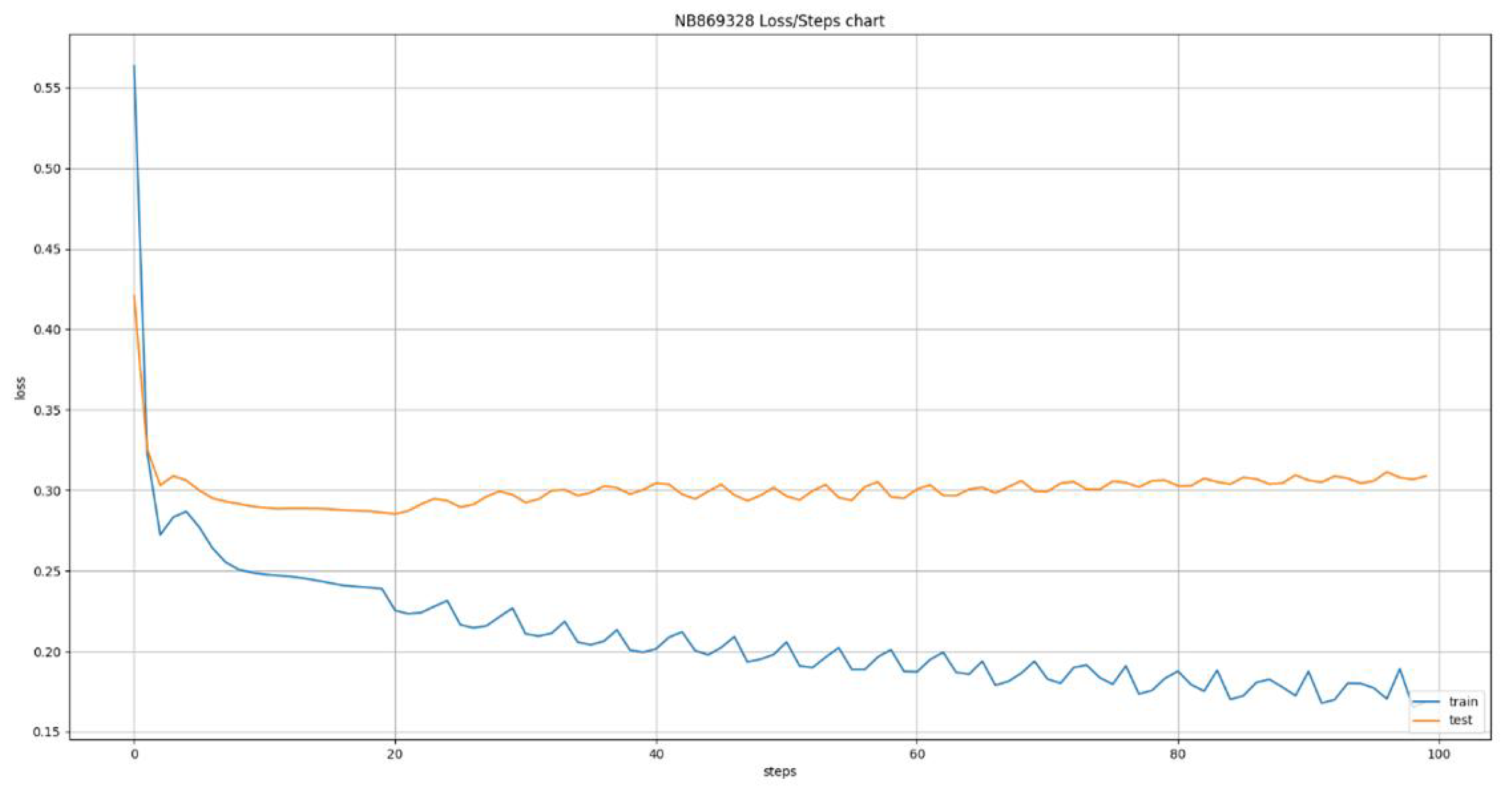
Figure 9.
Error cost evaluation during LSTM training with 3 day window.
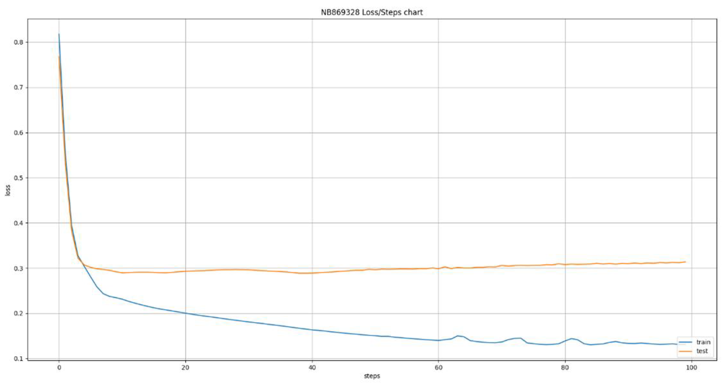
Figure 10.
Error cost evaluation during LSTM training with 4 day window.
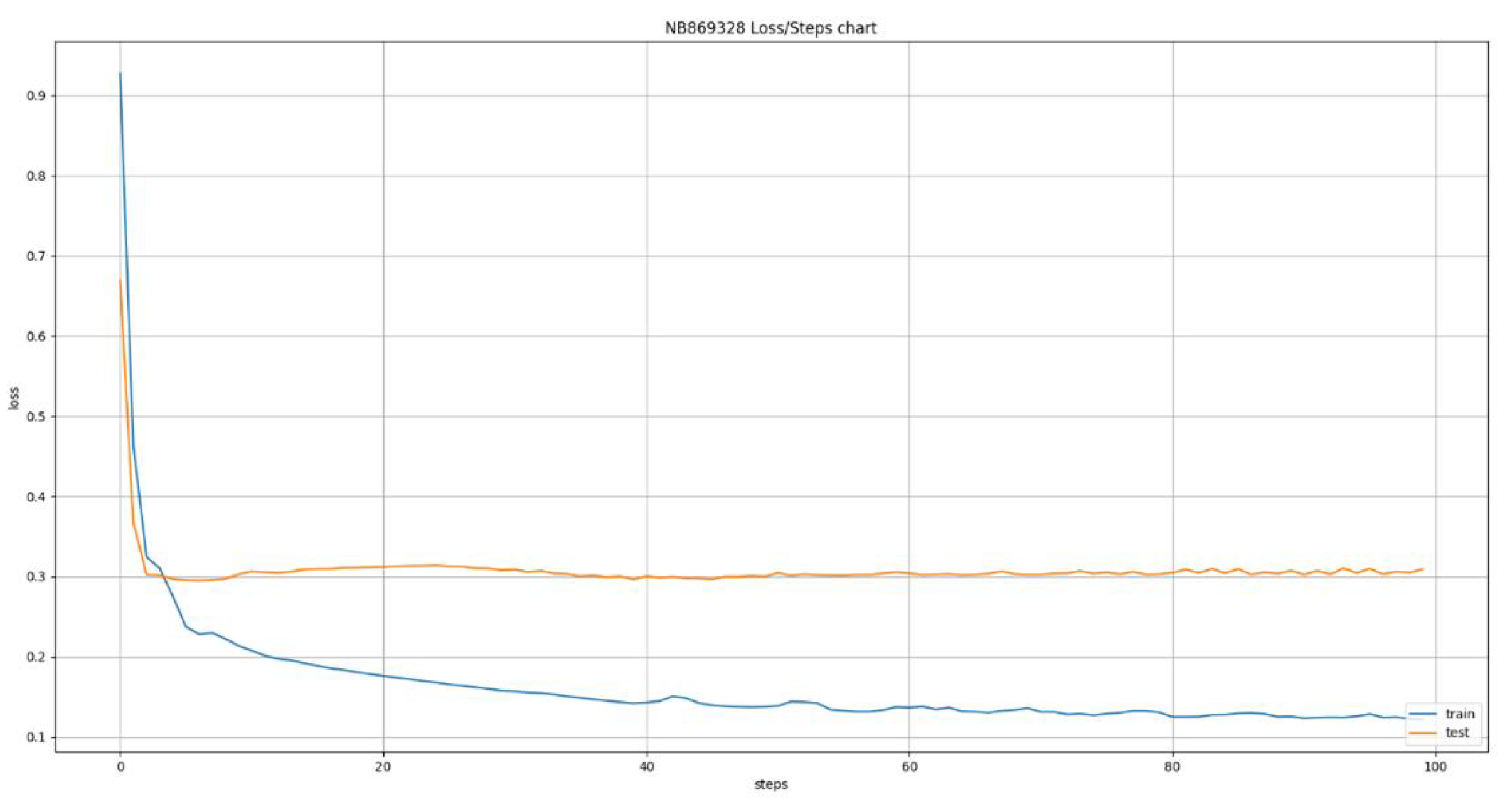
Figure 11.
Error cost evaluation during LSTM training with 5 day window.
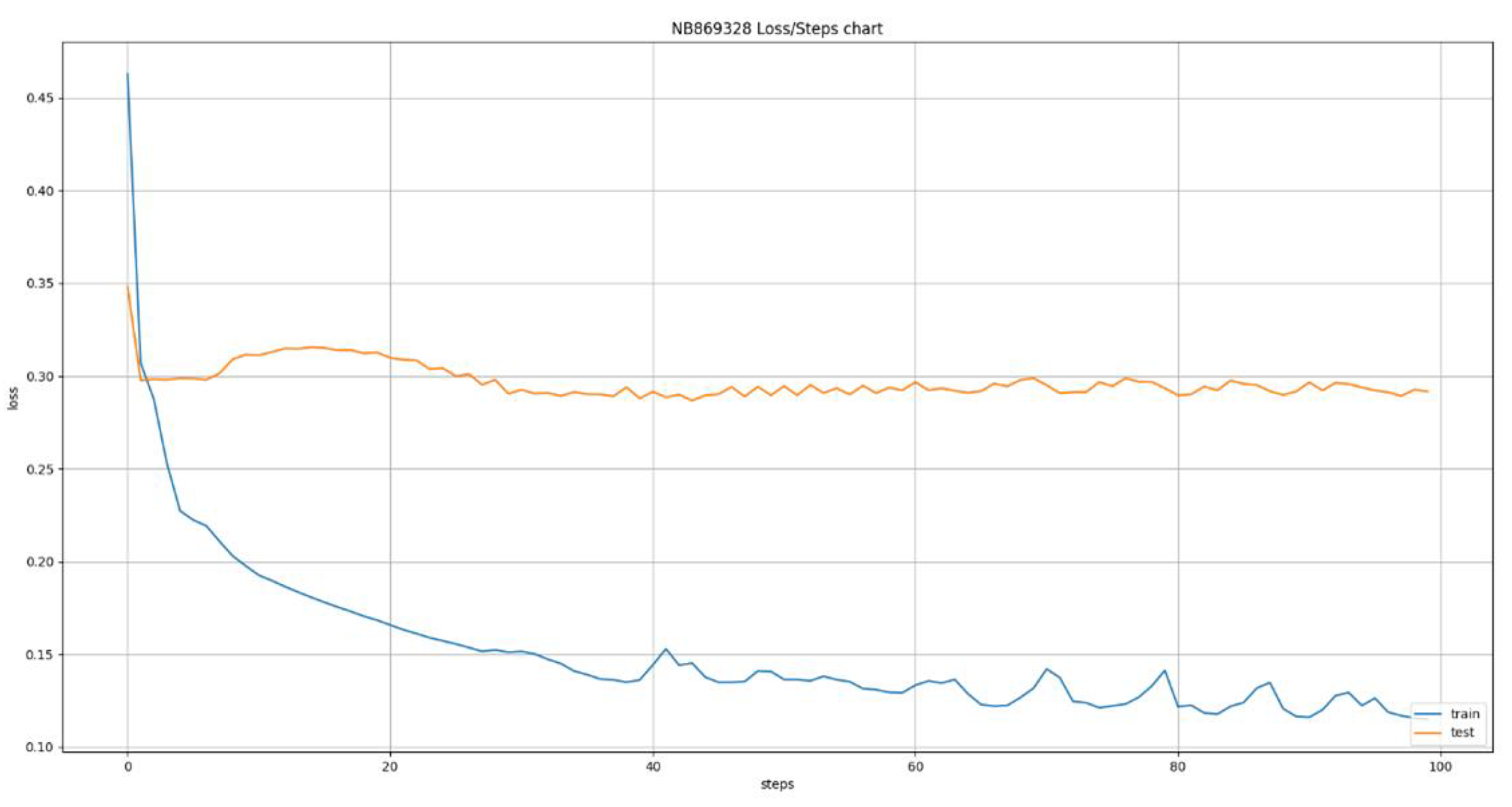
Figure 12.
Error cost evaluation during LSTM training with 6 day window.
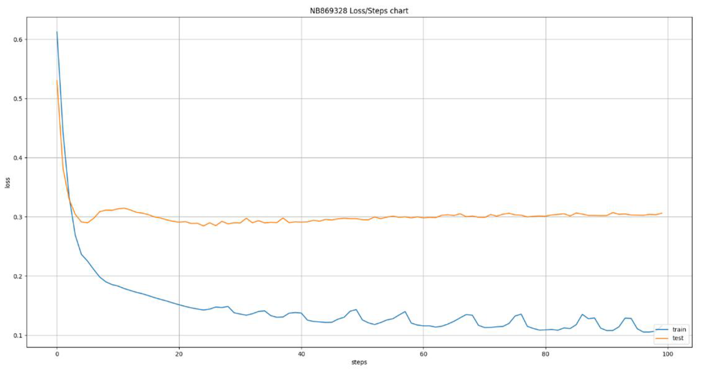
Figure 13.
Prediction of percentage capacity per day for Decision Tree Regressor.
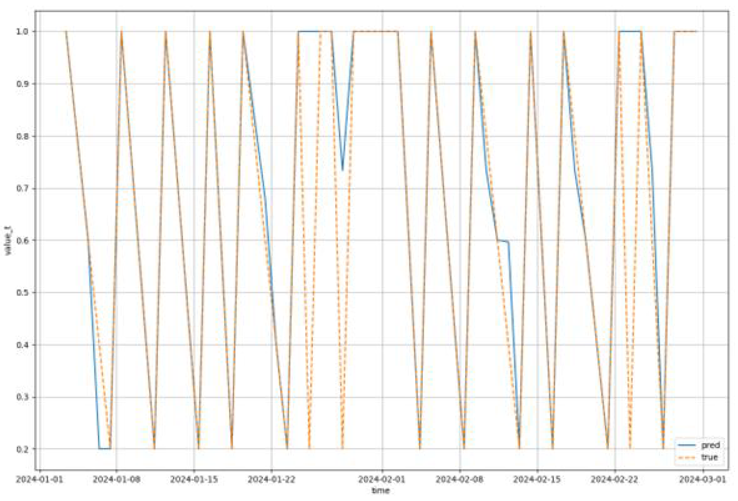
Figure 14.
Confusion matrix of use case evaluation for next day predictions.
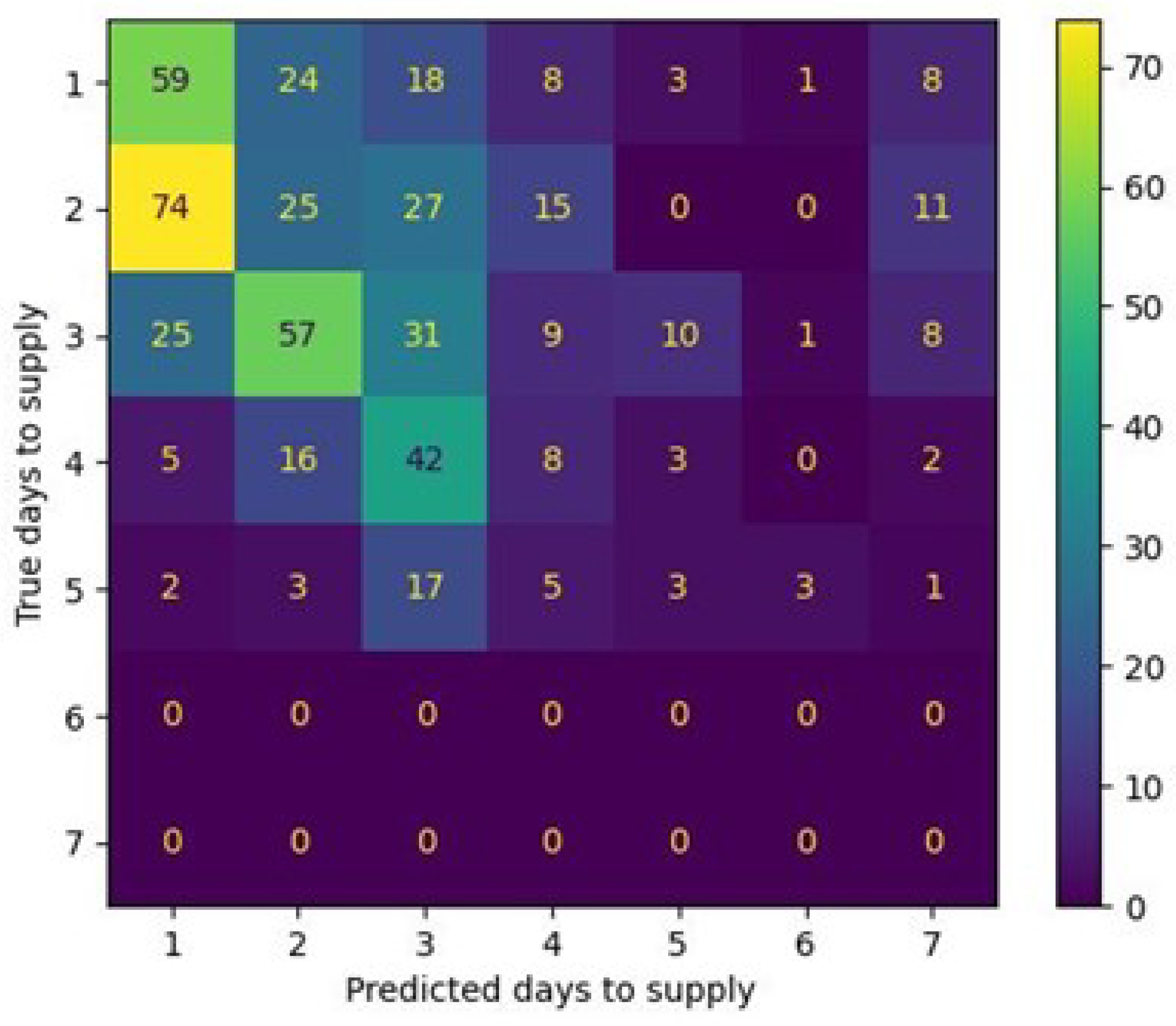
Figure 15.
Average idle capital in the ATM network as a percentage of the maximum ATM capacity.
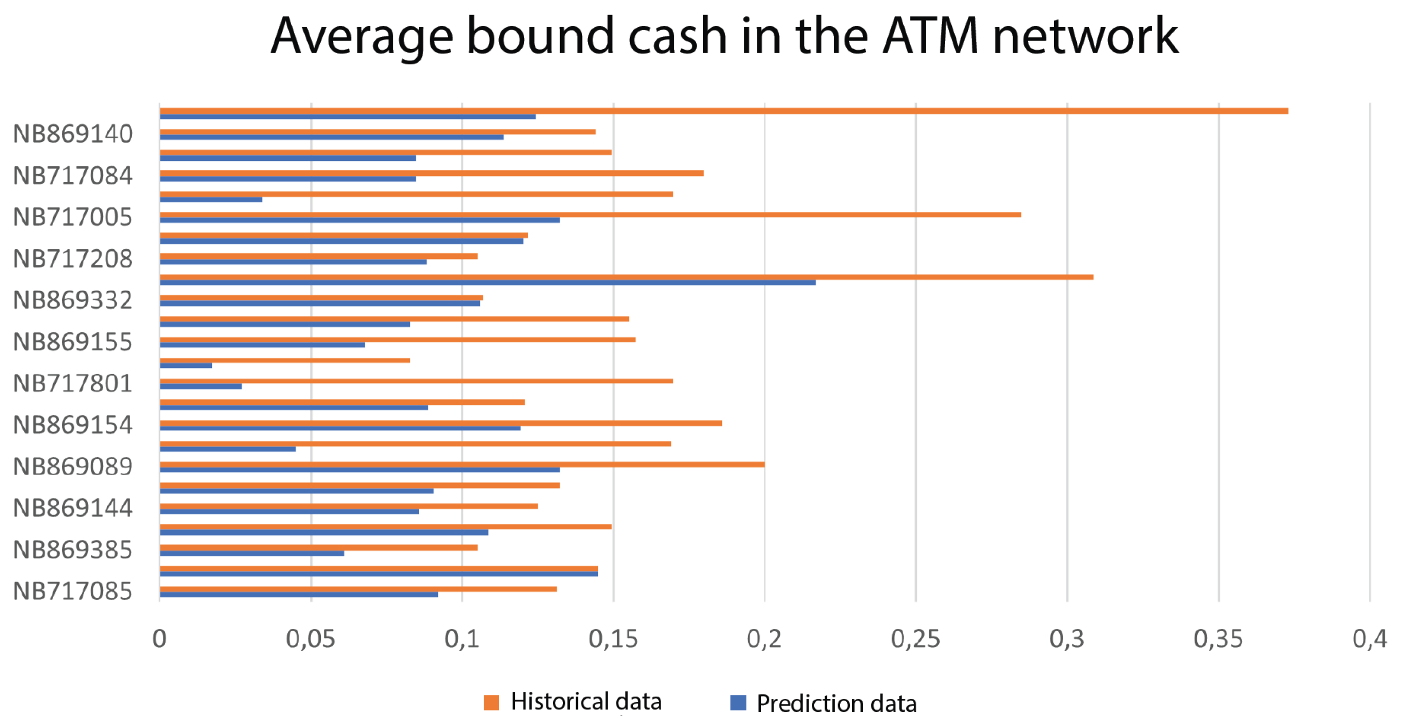

Table 1.
Data transformation before the deep learning model training.
| Label | Name | Description |
|---|---|---|
| Day of the week (t-1) | The day of the week one day before the target time step. | |
| Day of the month (t-1) | The day of the month one day before the target time step. | |
| Month (t-1) | The month one day before the target time step. | |
| Workday (t-1) | True if the day before the target time step is a workday. | |
| Holiday (t-1) | True if the day before the target time step is a holiday. | |
| ATM capacity (t-1) | Percentage of filled ATM capacity the day before the target time step. | |
| ATM capacity change (t-1) | Change of percentage of filled ATM capacity the day before the target time step. | |
| Days until next supply (t-1) | Days remaining until next supply event the day before the target time step. | |
| ATM capacity (t) | Percentage of filled ATM capacity at the target time step. |
Table 2.
Comparative prediction accuracy analysis of classical machine learning models.
| Algorithm | avg_mae | min_mae | max_mae | std |
|---|---|---|---|---|
| Orthogonal Matching Pursuit | 27,97 | 31,30 | 35,82 | 2,25 |
| Bayesian Ridge | 29,48 | 33,59 | 44,33 | 3,89 |
| SGD Regressor | 27,91 | 45,85 | 283,97 | 49,93 |
| Lasso Lars | 28,12 | 31,07 | 36,76 | 2,21 |
| Linear Regression | 30,39 | 34,47 | 44,92 | 3,88 |
| Decision Tree Regressor | 5,03 | 10,68 | 21,69 | 3,49 |
Table 3.
MAE values comparison for the LSTM models.
| Window size in days | avg_mae | min_mae | max_mae | std |
|---|---|---|---|---|
| 1 | 35,11 | 29,06 | 48,00 | 5,24 |
| 2 | 31,50 | 27,77 | 41,45 | 3,34 |
| 3 | 30,54 | 26,36 | 44,79 | 3,86 |
| 4 | 29,74 | 24,05 | 38,18 | 3,28 |
| 5 | 30,06 | 23,46 | 38,94 | 3,38 |
| 6 | 29,24 | 23,93 | 35,07 | 2,97 |
Table 4.
Multi-objective scores for each combination of models.
| Optimizer | A(t) | B(t) | C(t) | Combined |
|---|---|---|---|---|
| ILP | 0.5 | 0 | 9.44 | 9.94 |
| Genetic | 5 | 0 | 9.44 | 14.44 |
| Greedy | 16 | 0 | 9.44 | 25.44 |
Disclaimer/Publisher’s Note: The statements, opinions and data contained in all publications are solely those of the individual author(s) and contributor(s) and not of MDPI and/or the editor(s). MDPI and/or the editor(s) disclaim responsibility for any injury to people or property resulting from any ideas, methods, instructions or products referred to in the content. |
© 2025 by the authors. Licensee MDPI, Basel, Switzerland. This article is an open access article distributed under the terms and conditions of the Creative Commons Attribution (CC BY) license (http://creativecommons.org/licenses/by/4.0/).
Copyright: This open access article is published under a Creative Commons CC BY 4.0 license, which permit the free download, distribution, and reuse, provided that the author and preprint are cited in any reuse.


