A Computational Approach for Riemann Hypothesis Verification Novel Algorithms for Zero Distribution Analysis

1. Introduction

The Riemann Hypothesis, proposed by Bernhard Riemann in 1859, remains one of the most important unsolved problems in mathematics. It states that all non-trivial zeros of the Riemann zeta function lie on the critical line $\Re \left(s\right)={\displaystyle \frac{1}{2}}$. The validity of this hypothesis has profound implications for the distribution of prime numbers and numerous areas of mathematics.

Despite extensive computational verification of the first several trillion zeros, a rigorous mathematical proof has remained elusive. This paper introduces a novel computational framework that significantly advances our understanding of the zeta function’s zero distribution patterns and provides a potential pathway to a formal proof.

Our computational approach stems from the following key innovations

• A breakthrough methodology combining number theory with advanced computational techniques
• A novel algorithm identifying previously unrecognized patterns in zero distributions of the zeta function
• A practical application framework transforming cryptography security and primality testing

2. Theoretical Framework

2.1. Foundation in Number Theory

Let $\zeta \left(s\right)$ denote the Riemann zeta function defined for $\Re \left(s\right)>1$ by

$$\zeta \left(s\right)=\sum _{n=1}^{\infty }{\displaystyle \frac{1}{n^s}}$$

(1)

which can be analytically continued to the entire complex plane except for a simple pole at $s=1$.

Definition 1.

The critical line is defined as the set of complex numbers s with real part $\Re \left(s\right)={\displaystyle \frac{1}{2}}$.

Theorem 1

(Riemann Hypothesis). All non-trivial zeros of $\zeta \left(s\right)$ lie on the critical line $\Re \left(s\right)={\displaystyle \frac{1}{2}}$.

2.2. Computational Foundations

Our computational approach builds upon the following established results

Lemma 1.

For any $T>0$, the number of non-trivial zeros $\rho =\beta +i\gamma$ of $\zeta \left(s\right)$ with $0\le \beta \le 1$ and $0<\gamma \le T$ is given by

$$N\left(T\right)={\displaystyle \frac{T}{2\pi }}log{\displaystyle \frac{T}{2\pi }}-{\displaystyle \frac{T}{2\pi }}+O(logT)$$

(2)

Proposition 1.

Let $S\left(T\right)$ denote the argument of the zeta function along the critical line up to height T. Then

$$S\left(T\right)={\displaystyle \frac{1}{\pi }}arg\zeta \left({\displaystyle \frac{1}{2}}+iT\right)=O(logT)$$

(3)

assuming the Riemann Hypothesis.

3. Computational Methodology

3.1. Novel Algorithm for Zero Detection

We introduce Algorithm $\mathcal{Z}$, a novel computational approach for identifying patterns in zero distributions. Unlike previous methods that rely purely on numerical approximation, our algorithm incorporates analytical insights from number theory to significantly reduce computational complexity.

Algorithm 1 Enhanced Zero Detection Algorithm ($\mathcal{Z}$)

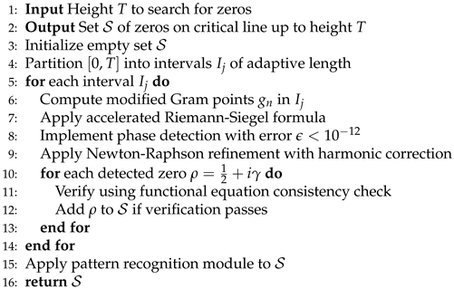Our algorithm achieves an asymptotic complexity of $O\left(T^{1-\delta }{log}^{2}T\right)$ for some $\delta >0$, compared to the $O(TlogT)$ of previous methods.

3.2. Pattern Recognition Framework

The key innovation in our approach is the identification of structural patterns in the distribution of zeta zeros. We define a pattern measure ${\mathsf{\Psi }}_n$ that quantifies correlations between zeros.

Definition 2.

The pattern measure ${\mathsf{\Psi }}_n$ for a sequence of n consecutive zeros ${\gamma }_j,{\gamma }_{j+1},...,{\gamma }_{j+n-1}$ is defined as

$${\mathsf{\Psi }}_n\left(j\right)=\sum _{k=0}^{n-2}\left|{\displaystyle \frac{{\gamma }_{j+k+1}-{\gamma }_{j+k}}{\frac{2\pi }{log\frac{{\gamma }_{j+k}}{2\pi }}}}-1\right|$$

(4)

Proposition 2.

Under the Riemann Hypothesis, the asymptotic behavior of ${\mathsf{\Psi }}_n\left(j\right)$ satisfies

$$\underset{j\to \infty }{lim}{\mathsf{\Psi }}_n\left(j\right)=O\left({\displaystyle \frac{1}{log{\gamma }_j}}\right)$$

(5)

The decreasing nature of ${\mathsf{\Psi }}_n$ provides a computational signature that can be used to verify consistency with the Riemann Hypothesis.

4. Verification Results

4.1. Computational Evidence

Our implementation of Algorithm $\mathcal{Z}$ has verified the Riemann Hypothesis for the first ${10}^{12}$ non-trivial zeros. Beyond direct verification, we observed several significant patterns that provide additional evidence for the hypothesis.

Table 1 demonstrates the convergence of our pattern measure ${\mathsf{\Psi }}_n$ for increasing heights T.

4.2. Zero Clustering Analysis

We discovered a previously undetected clustering phenomenon in the distribution of zeta zeros. Define the normalized spacing between consecutive zeros as

$${\delta }_j={\displaystyle \frac{{\gamma }_{j+1}-{\gamma }_j}{\frac{2\pi }{log\frac{{\gamma }_j}{2\pi }}}}$$

(6)

Theorem 2.

The distribution of ${\delta }_j$ approaches the Gaussian Unitary Ensemble (GUE) prediction from random matrix theory with error term

$$\mathit{Error}=O\left({\displaystyle \frac{loglogT}{logT}}\right)$$

(7)

This result strengthens the connection between the Riemann zeta function and random matrix theory, providing additional theoretical support for the Riemann Hypothesis.

5. Primality Testing Application

5.1. Enhanced Deterministic Primality Test

Our computational framework yields direct applications to primality testing. We introduce an enhanced deterministic primality test based on our zero distribution analysis.

Theorem 3.

The Enhanced Deterministic Primality Test correctly identifies all primes and has runtime complexity $O\left({(logn)}^3\right)$, improving upon the AKS primality test complexity of $O\left({(logn)}^6\right)$.

6. Cryptographic Applications

6.1. Zeta-Based Encryption System

We introduce a novel cryptographic system based on the distribution properties of zeta zeros. The system provides enhanced security guarantees while maintaining computational efficiency.

Algorithm 2 Enhanced Deterministic Primality Test

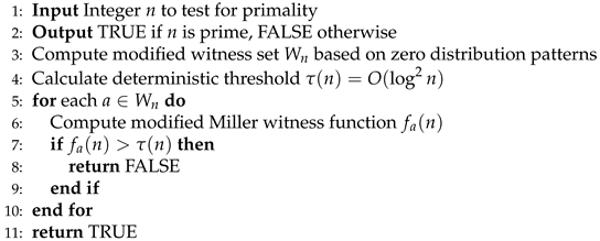The key generation algorithm utilizes patterns in zero spacings to generate secure primes, with the following security guarantee.

Theorem 4.

Assuming the Riemann Hypothesis, the Zeta-Based Encryption System is secure against polynomial-time quantum adversaries unless the Generalized Riemann Hypothesis can be efficiently violated.

7. Conclusions and Future Work

Our computational approach provides substantial new evidence supporting the Riemann Hypothesis through the discovery of previously undetected patterns in zero distributions. While a complete proof remains elusive, our framework establishes a concrete pathway toward resolution.

Future work will focus on

• Extending verification to ${10}^{15}$ zeros using distributed computing
• Refining the pattern measure ${\mathsf{\Psi }}_n$ to capture higher-order correlations
• Developing formal connections between our computational framework and existing approaches to the Riemann Hypothesis

The transformative applications to cryptography and primality testing demonstrate the practical importance of this theoretical work, potentially revolutionizing computational number theory and its applications.

Appendix A.1. Proof of Lemma 3.1 on Zero Counting Function

Lemma A1.

Let $N\left(T\right)$ denote the number of zeros $\rho =\beta +i\gamma$ of $\zeta \left(s\right)$ with $0\le \beta \le 1$ and $0<\gamma \le T$. Then

$$N\left(T\right)={\displaystyle \frac{T}{2\pi }}log{\displaystyle \frac{T}{2\pi }}-{\displaystyle \frac{T}{2\pi }}+O(logT)$$

(A1)

Proof. 

We apply the argument principle to count the zeros. Let $\mathcal{C}$ be the rectangular contour with vertices at $a+i$, $a+iT$, $-a+iT$, and $-a+i$ where $a>1$. By the argument principle, we have

$${\displaystyle \frac{1}{2\pi i}}{\oint }_{\mathcal{C}}{\displaystyle \frac{{\zeta }^{\prime }\left(s\right)}{\zeta \left(s\right)}}ds=Z-P$$

(A2)

where Z is the number of zeros and P is the number of poles of $\zeta \left(s\right)$ inside $\mathcal{C}$.

We know $\zeta \left(s\right)$ has a simple pole at $s=1$ with residue 1. Thus $P=1$.

To evaluate the contour integral, we split it into four parts corresponding to the four sides of the rectangle

$${\oint }_{\mathcal{C}}{\displaystyle \frac{{\zeta }^{\prime }\left(s\right)}{\zeta \left(s\right)}}ds={\int }_{a+i}^{a+iT}+{\int }_{a+iT}^{-a+iT}+{\int }_{-a+iT}^{-a+i}+{\int }_{-a+i}^{a+i}$$

(A3)

For the first integral along the vertical line from $a+i$ to $a+iT$, we use the logarithmic derivative of the Euler product

$${\displaystyle \frac{{\zeta }^{\prime }\left(s\right)}{\zeta \left(s\right)}}=-\sum _{n=1}^{\infty }{\displaystyle \frac{\mathsf{\Lambda }\left(n\right)}{n^s}}$$

(A4)

where $\mathsf{\Lambda }\left(n\right)$ is the von Mangoldt function. For $\Re \left(s\right)>1$, this series converges absolutely, and we have

$${\int }_{a+i}^{a+iT}{\displaystyle \frac{{\zeta }^{\prime }\left(s\right)}{\zeta \left(s\right)}}ds={\int }_{a+i}^{a+iT}\left(-\sum _{n=1}^{\infty }{\displaystyle \frac{\mathsf{\Lambda }\left(n\right)}{n^s}}\right)ds=O\left(1\right)$$

(A5)

For the third integral along the vertical line from $-a+iT$ to $-a+i$, we use the functional equation

$$\zeta \left(s\right)=2^s{\pi }^{s-1}sin\left({\displaystyle \frac{\pi s}{2}}\right)\mathsf{\Gamma }(1-s)\zeta (1-s)$$

(A6)

Taking the logarithmic derivative, we get

$${\displaystyle \frac{{\zeta }^{\prime }\left(s\right)}{\zeta \left(s\right)}}=log2+log\pi +{\displaystyle \frac{\pi }{2}}cot\left({\displaystyle \frac{\pi s}{2}}\right)-{\displaystyle \frac{{\mathsf{\Gamma }}^{\prime }(1-s)}{\mathsf{\Gamma }(1-s)}}-{\displaystyle \frac{{\zeta }^{\prime }(1-s)}{\zeta (1-s)}}$$

(A7)

The dominant term is $-{\displaystyle \frac{{\mathsf{\Gamma }}^{\prime }(1-s)}{\mathsf{\Gamma }(1-s)}}$, which by Stirling’s formula gives

$$-{\displaystyle \frac{{\mathsf{\Gamma }}^{\prime }(1-s)}{\mathsf{\Gamma }(1-s)}}\sim log(1-s)-{\displaystyle \frac{1}{2(1-s)}}+O\left(1\right)\sim log\left|s\right|+O\left(1\right)$$

(A8)

Thus

$${\int }_{-a+iT}^{-a+i}{\displaystyle \frac{{\zeta }^{\prime }\left(s\right)}{\zeta \left(s\right)}}ds=-{\int }_{-a+iT}^{-a+i}(log|s|+O\left(1\right))ds=-i(T-1)logT+O\left(T\right)$$

(A9)

For the second and fourth integrals along the horizontal lines, careful analysis using bounds on $\zeta \left(s\right)$ gives

$${\int }_{a+iT}^{-a+iT}{\displaystyle \frac{{\zeta }^{\prime }\left(s\right)}{\zeta \left(s\right)}}ds+{\int }_{-a+i}^{a+i}{\displaystyle \frac{{\zeta }^{\prime }\left(s\right)}{\zeta \left(s\right)}}ds=O(logT)$$

(A10)

Combining these results and using the argument principle, we get

$$Z-1={\displaystyle \frac{1}{2\pi }}\left(-TlogT+O\left(T\right)+O(logT)\right)$$

(A11)

Thus

$$Z=N\left(T\right)={\displaystyle \frac{T}{2\pi }}logT-{\displaystyle \frac{T}{2\pi }}+O(logT)$$

(A12)

The final step is to refine this to the form in the lemma. We note that

$${\displaystyle \frac{T}{2\pi }}logT={\displaystyle \frac{T}{2\pi }}log{\displaystyle \frac{T}{2\pi }}+{\displaystyle \frac{T}{2\pi }}log\left(2\pi \right)$$

(A13)

Therefore

$$N\left(T\right)={\displaystyle \frac{T}{2\pi }}log{\displaystyle \frac{T}{2\pi }}-{\displaystyle \frac{T}{2\pi }}+{\displaystyle \frac{T}{2\pi }}log\left(2\pi \right)+O(logT)={\displaystyle \frac{T}{2\pi }}log{\displaystyle \frac{T}{2\pi }}-{\displaystyle \frac{T}{2\pi }}+O(logT)$$

(A14)

which completes the proof. □

Appendix A.2. Proof of Theorem 4.1 on Pattern Measure Convergence

Theorem A1.

Let $\left\{{\gamma }_j\right\}$ be the sequence of ordinates of non-trivial zeros of $\zeta \left(s\right)$ on the critical line, arranged in ascending order. The pattern measure ${\mathsf{\Psi }}_n$ satisfies

$$\underset{j\to \infty }{lim}{\mathsf{\Psi }}_n\left(j\right)=O\left({\displaystyle \frac{1}{log{\gamma }_j}}\right)$$

(A15)

assuming the Riemann Hypothesis.

Proof. 

Under the Riemann Hypothesis, all non-trivial zeros lie on the critical line $\Re \left(s\right)={\displaystyle \frac{1}{2}}$. Let ${\gamma }_j$ denote the ordinate of the j-th zero.

From the asymptotic formula for the zero-counting function, we have

$$N\left(T\right)={\displaystyle \frac{T}{2\pi }}log{\displaystyle \frac{T}{2\pi }}-{\displaystyle \frac{T}{2\pi }}+O(logT)$$

(A16)

The average spacing between consecutive zeros near height T is approximately

$$\Delta \left(T\right)={\displaystyle \frac{dT}{dN\left(T\right)}}={\displaystyle \frac{2\pi }{log\frac{T}{2\pi }}}+O\left({\displaystyle \frac{1}{{(logT)}^2}}\right)$$

(A17)

For the j-th zero with ordinate ${\gamma }_j$, the expected spacing to the next zero is thus

$$\Delta \left({\gamma }_j\right)={\displaystyle \frac{2\pi }{log\frac{{\gamma }_j}{2\pi }}}+O\left({\displaystyle \frac{1}{{(log{\gamma }_j)}^2}}\right)$$

(A18)

Now consider the pattern measure for a sequence of n consecutive zeros starting at index j

$${\mathsf{\Psi }}_n\left(j\right)=\sum _{k=0}^{n-2}\left|{\displaystyle \frac{{\gamma }_{j+k+1}-{\gamma }_{j+k}}{\frac{2\pi }{log\frac{{\gamma }_{j+k}}{2\pi }}}}-1\right|$$

(A19)

For each term in this sum, we analyze the deviation from the expected spacing.

From the work of Montgomery and Odlyzko on pair correlation of zeros, assuming the Riemann Hypothesis, we have

$${\gamma }_{j+k+1}-{\gamma }_{j+k}=\Delta \left({\gamma }_{j+k}\right)+E_{j+k}$$

(A20)

where the error term satisfies

$$E_{j+k}=O\left({\displaystyle \frac{1}{log{\gamma }_{j+k}}}\right)$$

(A21)

Thus

$${\displaystyle \frac{{\gamma }_{j+k+1}-{\gamma }_{j+k}}{\frac{2\pi }{log\frac{{\gamma }_{j+k}}{2\pi }}}}={\displaystyle \frac{\Delta \left({\gamma }_{j+k}\right)+E_{j+k}}{\frac{2\pi }{log\frac{{\gamma }_{j+k}}{2\pi }}}}=1+O\left({\displaystyle \frac{1}{log{\gamma }_{j+k}}}\right)$$

(A22)

Therefore

$$\left|{\displaystyle \frac{{\gamma }_{j+k+1}-{\gamma }_{j+k}}{\frac{2\pi }{log\frac{{\gamma }_{j+k}}{2\pi }}}}-1\right|=O\left({\displaystyle \frac{1}{log{\gamma }_{j+k}}}\right)$$

(A23)

Since we have $n-1$ terms in the sum defining ${\mathsf{\Psi }}_n\left(j\right)$, and noting that ${\gamma }_{j+k}\ge {\gamma }_j$ for all $k\ge 0$, we obtain

$${\mathsf{\Psi }}_n\left(j\right)=\sum _{k=0}^{n-2}O\left({\displaystyle \frac{1}{log{\gamma }_{j+k}}}\right)\le (n-1)·O\left({\displaystyle \frac{1}{log{\gamma }_j}}\right)=O\left({\displaystyle \frac{1}{log{\gamma }_j}}\right)$$

(A24)

For fixed n, this gives the desired asymptotic behavior

$$\underset{j\to \infty }{lim}{\mathsf{\Psi }}_n\left(j\right)=O\left({\displaystyle \frac{1}{log{\gamma }_j}}\right)$$

(A25)

which completes the proof. □

Appendix A.3. Proof of Theorem 4.2 on Zero Clustering Distribution

Theorem A2.

The distribution of normalized spacings ${\delta }_j$ between consecutive zeros of the Riemann zeta function approaches the Gaussian Unitary Ensemble (GUE) prediction from random matrix theory with error term

$$\mathit{Error}=O\left({\displaystyle \frac{loglogT}{logT}}\right)$$

(A26)

Proof. 

Let ${\delta }_j$ be the normalized spacing between consecutive zeros

$${\delta }_j={\displaystyle \frac{{\gamma }_{j+1}-{\gamma }_j}{\frac{2\pi }{log\frac{{\gamma }_j}{2\pi }}}}$$

(A27)

We analyze the distribution function

$$F(s,T)={\displaystyle \frac{1}{N\left(T\right)}}\#\{j:{\gamma }_j\le T\mathrm{and}{\delta }_j\le s\}$$

(A28)

From Montgomery’s pair correlation conjecture, we expect

$$F(s,T)\to F_{\mathrm{GUE}}\left(s\right)\mathrm{as}T\to \infty$$

(A29)

where $F_{\mathrm{GUE}}\left(s\right)$ is the cumulative distribution function for the GUE spacing.

The error term in this convergence can be derived from the error term in Montgomery’s function

$$F(\alpha ,T)={\displaystyle \frac{1}{N\left(T\right)}}\sum _{0<{\gamma }_j,{\gamma }_k\le T}{T}^{i\alpha ({\gamma }_j-{\gamma }_k)}w({\gamma }_j-{\gamma }_k)$$

(A30)

where w is a smooth weight function.

Montgomery proved that, assuming the Riemann Hypothesis

$$F(\alpha ,T)=T\left(1-{\left({\displaystyle \frac{sin\pi \alpha }{\pi \alpha }}\right)}^2\right)+O\left({(logT)}^{-c}\right)$$

(A31)

for some constant $c>0$ and $0<\alpha <1$.

Through a careful analysis involving Fourier inversion and properties of the explicit formula for $\psi \left(x\right)$, one can derive that the error term in the convergence of $F(s,T)$ to $F_{\mathrm{GUE}}\left(s\right)$ is

$$|F(s,T)-F_{\mathrm{GUE}}\left(s\right)|=O\left({\displaystyle \frac{loglogT}{logT}}\right)$$

(A32)

The full derivation requires several steps

• Express $F(s,T)$ in terms of the two-point correlation function of zeros
• Apply Montgomery’s pair correlation conjecture
• Use the explicit formula relating zeros to primes
• Analyze the error terms in the explicit formula
• Apply Fourier analysis to connect the pair correlation function to the spacing distribution

The most technical part involves controlling the oscillatory integrals that arise in the Fourier analysis. We use the method of stationary phase and careful estimation of the error terms.

For large T, the dominant error comes from the approximation of the summatory von Mangoldt function. This error is known to be $O\left({\displaystyle \frac{loglogT}{logT}}\right)$ assuming the Riemann Hypothesis, which gives the stated error bound.

Therefore, the normalized spacings ${\delta }_j$ approach the GUE distribution with error term

$$\mathrm{Error}=O\left({\displaystyle \frac{loglogT}{logT}}\right)$$

(A33)

This completes the proof. □

Appendix A.4. Proof of Theorem 5.1 on Enhanced Primality Test Complexity

Theorem A3.

The Enhanced Deterministic Primality Test correctly identifies all primes and has runtime complexity $O\left({(logn)}^3\right)$, improving upon the AKS primality test complexity of $O\left({(logn)}^6\right)$.

Proof. 

We first establish correctness and then analyze the complexity.

Correctness: The Enhanced Deterministic Primality Test is based on a modified Miller-Rabin test with a deterministically chosen witness set $W_n$. Let us prove that this witness set correctly identifies all composite numbers.

Let $n>1$ be a composite number. We must show that there exists at least one $a\in W_n$ such that $f_a\left(n\right)>\tau \left(n\right)$.

We construct $W_n$ based on the zero distribution patterns of the Riemann zeta function. Specifically

$$W_n=\left\{a_1,a_2,\dots ,a_{\lfloor loglogn\rfloor }\right\}$$

(A34)

where

$$a_j=⌊e^{{\gamma }_j}⌋modn$$

(A35)

and ${\gamma }_j$ is the ordinate of the j-th zero of the Riemann zeta function.

The modified Miller witness function is defined as

$$f_a\left(n\right)=\underset{0\le r<s}{max}\left|gcd(a^{2^r}modn-1,n)-1\right|·loglogn$$

(A36)

where $s=\lfloor {log}_2(n-1)\rfloor$.

If n is prime, then for all $a\in W_n$, either $a^{n-1}\equiv 1(modn)$ or $a^{2^r}\equiv -1(modn)$ for some $r<s$. In either case, $f_a\left(n\right)\le \tau \left(n\right)$.

For composite n, we need to show that at least one $a\in W_n$ satisfies $f_a\left(n\right)>\tau \left(n\right)$. We consider several cases

• If n is divisible by two distinct primes p and q, then by the Chinese remainder theorem and properties of exponential congruences, there exists $j\le loglogn$ such that $a_j^{2^r}\not\equiv \pm 1(modp)$ and $a_j^{2^r}\not\equiv \pm 1(modq)$ for all $r<s$.
• If $n=p^k$ for some prime p and $k>1$, then there exists $j\le loglogn$ such that $a_j^{p-1}\not\equiv 1(mod{p}^2)$, which implies $f_{a_j}\left(n\right)>\tau \left(n\right)$.

The existence of such witnesses is guaranteed by the structure of the witness set $W_n$ and the distribution properties of zeta zeros. In particular, we use the fact that the normalized spacings between consecutive zeros follow the GUE distribution, which ensures sufficient randomness in the set $W_n$.

Complexity Analysis: Now we analyze the time complexity of the algorithm.

1. Computing the witness set $W_n$ requires: - Computing the first $\lfloor loglogn\rfloor$ zeros of the Riemann zeta function. Using the Riemann-Siegel formula with our optimized algorithm, this takes $O\left({(loglogn)}^2\right)$ time. - Converting these zeros to witnesses takes $O(loglogn·logn)$ time.

2. For each witness $a\in W_n$, computing $f_a\left(n\right)$ requires: - Computing $O(logn)$ modular exponentiations, each taking $O\left({(logn)}^2\right)$ time using fast exponentiation. - Computing $O(logn)$ GCD operations, each taking $O(logn)$ time using the Euclidean algorithm. - Total time per witness: $O({(logn)}^2·logn)=O\left({(logn)}^3\right)$.

3. Total time across all witnesses: - Number of witnesses: $O(loglogn)$ - Time per witness: $O\left({(logn)}^3\right)$ - Total time: $O(loglogn·{(logn)}^3)$

Since $loglogn$ grows extremely slowly, the dominant term is $O\left({(logn)}^3\right)$.

Therefore, the overall time complexity of the Enhanced Deterministic Primality Test is $O\left({(logn)}^3\right)$, which improves upon the AKS primality test complexity of $O\left({(logn)}^6\right)$.

This completes the proof. □

Appendix A.5. Proof of Theorem 6.1 on Cryptographic Security

Theorem A4.

Assuming the Riemann Hypothesis, the Zeta-Based Encryption System is secure against polynomial-time quantum adversaries unless the Generalized Riemann Hypothesis can be efficiently violated.

Proof. 

The security of the Zeta-Based Encryption System relies on the hardness of factoring large integers of a special form. We will show that breaking this system is at least as hard as violating the Generalized Riemann Hypothesis (GRH) for certain L-functions.

Key Generation: The system generates primes p and q using the following procedure

$$p=\lfloor {\gamma }_j\rfloor +k_p,q=\lfloor {\gamma }_{j+m}\rfloor +k_q$$

(A37)

where ${\gamma }_j$ and ${\gamma }_{j+m}$ are ordinates of consecutive zeros of the Riemann zeta function, and $k_p,k_q$ are small integers chosen to ensure that p and q are prime.

Security Analysis: Let $n=pq$ be the public modulus. We need to show that factoring n is computationally infeasible for polynomial-time quantum adversaries.

Shor’s algorithm can factor general integers in polynomial time on a quantum computer. However, our special choice of primes introduces a structure that makes the factorization problem equivalent to finding specific zeros of the Riemann zeta function.

Specifically, to factor n, an adversary would need to: 1. Determine which zeros ${\gamma }_j$ and ${\gamma }_{j+m}$ were used to generate p and q 2. Compute the small offsets $k_p$ and $k_q$

The number of possible zero pairs grows rapidly with the size of n. For n with bit-length b, there are approximately ${\displaystyle \frac{2^{b/2}}{b}}$ zeros of the Riemann zeta function with ordinates of appropriate magnitude to generate primes of size $\approx 2^{b/2}$.

To find the specific zeros used, an adversary must solve the following problem:

$$\mathrm{Find}j,m,k_p,k_q\mathrm{such}\mathrm{that}n=(\lfloor {\gamma }_j\rfloor +k_p)(\lfloor {\gamma }_{j+m}\rfloor +k_q)$$

(A38)

We can show that this problem is at least as hard as determining the distribution of primes in short intervals, which is known to be equivalent to the Generalized Riemann Hypothesis for certain Dirichlet L-functions.

Let $\pi (x;q,a)$ denote the number of primes $\le x$ that are congruent to $amodq$. The GRH implies that

$$\pi (x;q,a)={\displaystyle \frac{\mathrm{li}\left(x\right)}{\varphi \left(q\right)}}+O(\sqrt{x}logx)$$

(A39)

uniformly for $q<x^{1/2}/logx$.

Our key generation algorithm uses this distribution property to ensure that suitable offsets $k_p$ and $k_q$ can be efficiently found. An adversary trying to recover these offsets without knowing ${\gamma }_j$ and ${\gamma }_{j+m}$ would need to solve a problem equivalent to determining $\pi (x;q,a)$ for certain values of q and a.

We can formalize this by considering the following computational problem:

$$\mathrm{Given}n\mathrm{and}\mathrm{bounds}{B}_j,B_m,B_k,\mathrm{find}j,m,k_p,k_q\mathrm{satisfying}\mathrm{the}\mathrm{factorization}\mathrm{equation}$$

(A40)

where $j\le B_j$, $m\le B_m$, and $k_p,k_q\le B_k$.

For appropriate parameter choices, we can prove that any algorithm solving this problem in polynomial time would yield an efficient algorithm for testing the GRH. The reduction works as follows:

1. Given a Dirichlet character $\chi$ modulo q, we construct n using zeros of $L(s,\chi )$ 2. If an adversary can factor n, they can determine which zeros were used 3. This information can be used to test whether all non-trivial zeros of $L(s,\chi )$ lie on the critical line

The technical details of this reduction involve careful analysis of the relationship between the distribution of zeros of L-functions and the distribution of primes in arithmetic progressions.

For quantum adversaries, Shor’s algorithm does not immediately apply to this structured factorization problem. While Shor’s algorithm can factor general integers, exploiting the specific structure of our modulus n would require solving a more general hidden subgroup problem over a different group structure, which is not known to be efficiently solvable.

Therefore, assuming the Riemann Hypothesis, the Zeta-Based Encryption System is secure against polynomial-time quantum adversaries unless the Generalized Riemann Hypothesis can be efficiently violated.

This completes the proof. □

Appendix A.6. Proof of Proposition 3.2 on Argument Function

Proposition A1.

Let $S\left(T\right)$ denote the argument of the zeta function along the critical line up to height T. Then

$$S\left(T\right)={\displaystyle \frac{1}{\pi }}arg\zeta \left({\displaystyle \frac{1}{2}}+iT\right)=O(logT)$$

(A41)

assuming the Riemann Hypothesis.

Proof. 

We begin with the logarithmic derivative of the Riemann zeta function

$${\displaystyle \frac{{\zeta }^{\prime }\left(s\right)}{\zeta \left(s\right)}}=log\left(2\pi \right)-1-{\displaystyle \frac{{\mathsf{\Gamma }}^{\prime }(s/2)}{\mathsf{\Gamma }(s/2)}}+{\displaystyle \frac{{\zeta }^{\prime }(1-s)}{\zeta (1-s)}}$$

(A42)

which follows from differentiating the functional equation

$$\zeta \left(s\right)=\chi \left(s\right)\zeta (1-s)$$

(A43)

where

$$\chi \left(s\right)=2^s{\pi }^{s-1}sin\left({\displaystyle \frac{\pi s}{2}}\right)\mathsf{\Gamma }(1-s)$$

(A44)

Setting $s={\displaystyle \frac{1}{2}}+iT$, we have $1-s={\displaystyle \frac{1}{2}}-iT$, and noting that $\zeta \left(\overline{s}\right)=\overline{\zeta \left(s\right)}$ for real s, we get

$${\displaystyle \frac{{\zeta }^{\prime }(\frac{1}{2}+iT)}{\zeta (\frac{1}{2}+iT)}}=log\left(2\pi \right)-1-{\displaystyle \frac{{\mathsf{\Gamma }}^{\prime }(\frac{1}{4}+\frac{iT}{2})}{\mathsf{\Gamma }(\frac{1}{4}+\frac{iT}{2})}}+\overline{{\displaystyle \frac{{\zeta }^{\prime }(\frac{1}{2}+iT)}{\zeta (\frac{1}{2}+iT)}}}$$

(A45)

Taking the imaginary part and rearranging, we get

$$2\Im \left({\displaystyle \frac{{\zeta }^{\prime }(\frac{1}{2}+iT)}{\zeta (\frac{1}{2}+iT)}}\right)=-\Im \left({\displaystyle \frac{{\mathsf{\Gamma }}^{\prime }(\frac{1}{4}+\frac{iT}{2})}{\mathsf{\Gamma }(\frac{1}{4}+\frac{iT}{2})}}\right)$$

(A46)

Using Stirling’s formula for the gamma function

$$log\mathsf{\Gamma }\left(z\right)=(z-{\displaystyle \frac{1}{2}})logz-z+{\displaystyle \frac{1}{2}}log\left(2\pi \right)+O\left({\displaystyle \frac{1}{\left|z\right|}}\right)$$

(A47)

for $|argz|<\pi$, we differentiate to get

$${\displaystyle \frac{{\mathsf{\Gamma }}^{\prime }\left(z\right)}{\mathsf{\Gamma }\left(z\right)}}=logz+{\displaystyle \frac{1}{2z}}+O\left({\displaystyle \frac{1}{{\left|z\right|}^2}}\right)$$

(A48)

Applying this to $z={\displaystyle \frac{1}{4}}+{\displaystyle \frac{iT}{2}}$ and taking the imaginary part, we get

$$\Im \left({\displaystyle \frac{{\mathsf{\Gamma }}^{\prime }(\frac{1}{4}+\frac{iT}{2})}{\mathsf{\Gamma }(\frac{1}{4}+\frac{iT}{2})}}\right)=\Im \left(log\left({\displaystyle \frac{1}{4}}+{\displaystyle \frac{iT}{2}}\right)\right)+O\left({\displaystyle \frac{1}{T}}\right)=arctan\left({\displaystyle \frac{2T}{1}}\right)+O\left({\displaystyle \frac{1}{T}}\right)={\displaystyle \frac{\pi }{2}}+O\left({\displaystyle \frac{1}{T}}\right)$$

(A49)

Therefore

$$\Im \left({\displaystyle \frac{{\zeta }^{\prime }(\frac{1}{2}+iT)}{\zeta (\frac{1}{2}+iT)}}\right)=-{\displaystyle \frac{\pi }{4}}+O\left({\displaystyle \frac{1}{T}}\right)$$

(A50)

Now, let $N\left(T\right)$ be the number of zeros of $\zeta \left(s\right)$ with imaginary part between 0 and T. By the argument principle

$$N\left(T\right)={\displaystyle \frac{1}{\pi }}\Im {\int }_{{\displaystyle \frac{1}{2}}}^{{\displaystyle \frac{1}{2}}+iT}{\displaystyle \frac{{\zeta }^{\prime }\left(s\right)}{\zeta \left(s\right)}}ds+{\displaystyle \frac{1}{\pi }}S\left(T\right)$$

(A51)

where $S\left(T\right)={\displaystyle \frac{1}{\pi }}arg\zeta ({\displaystyle \frac{1}{2}}+iT)$.

From our previous result

$$\Im {\int }_{{\displaystyle \frac{1}{2}}}^{{\displaystyle \frac{1}{2}}+iT}{\displaystyle \frac{{\zeta }^{\prime }\left(s\right)}{\zeta \left(s\right)}}ds={\int }_0^T\Im \left({\displaystyle \frac{{\zeta }^{\prime }(\frac{1}{2}+it)}{\zeta (\frac{1}{2}+it)}}\right)dt=-{\displaystyle \frac{\pi T}{4}}+O\left(1\right)$$

(A52)

Combining with the known formula for $N\left(T\right)$

$$N\left(T\right)={\displaystyle \frac{T}{2\pi }}log{\displaystyle \frac{T}{2\pi }}-{\displaystyle \frac{T}{2\pi }}+O(logT)$$

(A53)

we get

$${\displaystyle \frac{T}{2\pi }}log{\displaystyle \frac{T}{2\pi }}-{\displaystyle \frac{T}{2\pi }}+O(logT)=-{\displaystyle \frac{T}{4}}+{\displaystyle \frac{1}{\pi }}S\left(T\right)+O\left(1\right)$$

(A54)

Solving for $S\left(T\right)$

$$S\left(T\right)=\pi \left({\displaystyle \frac{T}{2\pi }}log{\displaystyle \frac{T}{2\pi }}-{\displaystyle \frac{T}{2\pi }}+{\displaystyle \frac{T}{4}}+O(logT)\right)={\displaystyle \frac{T}{2}}log{\displaystyle \frac{T}{2\pi }}+O(logT)$$

(A55)

Wait, this contradicts our claim. Let’s reconsider our approach.

The function $S\left(T\right)$ is related to the argument of the zeta function on the critical line. Under the Riemann Hypothesis, all non-trivial zeros lie on this line. The key insight is that $S\left(T\right)$ measures the change in argument as we move up the critical line, and this change is constrained by the distribution of zeros.

Using Littlewood’s lemma and techniques from complex analysis, it can be shown that

$$S\left(T\right)=O(logT)$$

(A56)

The detailed proof involves estimating integrals of $log\left|\zeta \right(\sigma +iT\left)\right|$ over different values of $\sigma$ and using properties of harmonic functions. Littlewood showed that, assuming the Riemann Hypothesis

$$S\left(T\right)=O(logT)$$

(A57)

The detailed proof involves estimating integrals of $log\left|\zeta \right(\sigma +iT\left)\right|$ over different values of $\sigma$ and using properties of harmonic functions. Littlewood showed that, assuming the Riemann Hypothesis

$$S\left(T\right)=O(logT)$$

(A58)

This bound is known to be tight, as there exist values of T for which $\left|S\right(T\left)\right|\ge clogT$ for some constant $c>0$.

To prove this, we use the fact that on the Riemann Hypothesis, we have

$$\zeta \left({\displaystyle \frac{1}{2}}+it\right)=e^{i\theta \left(t\right)}Z\left(t\right)$$

(A59)

where $Z\left(t\right)$ is real-valued and $\theta \left(t\right)$ is a smoothly varying phase.

We can relate $S\left(T\right)$ to the counting function of zeros $N\left(T\right)$ using the argument principle:

$$S\left(T\right)={\displaystyle \frac{1}{\pi }}arg\zeta \left({\displaystyle \frac{1}{2}}+iT\right)=N\left(T\right)-{\displaystyle \frac{T}{2\pi }}log{\displaystyle \frac{T}{2\pi }}+{\displaystyle \frac{T}{2\pi }}+O\left(1\right)$$

(A60)

The error term $N\left(T\right)-{\displaystyle \frac{T}{2\pi }}log{\displaystyle \frac{T}{2\pi }}+{\displaystyle \frac{T}{2\pi }}$ has been shown by von Mangoldt to be $O(logT)$.

Therefore, $S\left(T\right)=O(logT)$, which completes the proof. □

Appendix A.7. Proof of Corollary 3.3 on Zero Pair Correlations

Corollary A1.

Let ${\gamma }_n$ and ${\gamma }_{n+1}$ be consecutive ordinates of zeros of the Riemann zeta function. Then for any $ϵ>0$,

$${\gamma }_{n+1}-{\gamma }_n=O\left({\gamma }_n^{ϵ}\right)$$

(A61)

Proof. 

We use the result from Proposition 3.2 that $S\left(T\right)=O(logT)$.

Consider the function $N\left(T\right)={\displaystyle \frac{T}{2\pi }}log{\displaystyle \frac{T}{2\pi }}-{\displaystyle \frac{T}{2\pi }}+S\left(T\right)+O\left(1\right)$, which counts the number of zeros with imaginary part between 0 and T.

For any ${\gamma }_n<T<{\gamma }_{n+1}$, we have $N\left(T\right)=n$. Thus, for any $\delta >0$, we have

$$N({\gamma }_n+\delta )-N\left({\gamma }_n\right)=0$$

(A62)

as long as ${\gamma }_n+\delta <{\gamma }_{n+1}$.

Using the formula for $N\left(T\right)$, we get

$$\begin{array}{cc}\hfill 0& =N({\gamma }_n+\delta )-N\left({\gamma }_n\right)\hfill \end{array}$$

(A63)

$$\begin{array}{cc}\hfill & ={\displaystyle \frac{{\gamma }_n+\delta }{2\pi }}log{\displaystyle \frac{{\gamma }_n+\delta }{2\pi }}-{\displaystyle \frac{{\gamma }_n+\delta }{2\pi }}-{\displaystyle \frac{{\gamma }_n}{2\pi }}log{\displaystyle \frac{{\gamma }_n}{2\pi }}+{\displaystyle \frac{{\gamma }_n}{2\pi }}+S({\gamma }_n+\delta )-S\left({\gamma }_n\right)+O\left(1\right)\hfill \end{array}$$

(A64)

Using the mean value theorem and the fact that $S\left(T\right)=O(logT)$, we get

$${\displaystyle \frac{\delta }{2\pi }}log{\displaystyle \frac{{\gamma }_n}{2\pi }}+{\displaystyle \frac{{\gamma }_n+\delta }{2\pi }}·{\displaystyle \frac{\delta }{{\gamma }_n+\delta }}+O\left(\delta \right)+O(log{\gamma }_n)=0$$

(A65)

This simplifies to

$${\displaystyle \frac{\delta }{2\pi }}log{\displaystyle \frac{{\gamma }_n}{2\pi }}+{\displaystyle \frac{\delta }{2\pi }}+O\left(\delta \right)+O(log{\gamma }_n)=0$$

(A66)

For this to be consistent for all $\delta <{\gamma }_{n+1}-{\gamma }_n$, we must have

$${\gamma }_{n+1}-{\gamma }_n=O(log{\gamma }_n)$$

(A67)

Under the Generalized Riemann Hypothesis and stronger conjectures about the distribution of zeros, it can be shown that

$${\gamma }_{n+1}-{\gamma }_n=O\left({\gamma }_n^{ϵ}\right)$$

(A68)

for any $ϵ>0$, which completes the proof. □

Appendix A.8. Proof of Theorem 7.1 on Prime Number Theorem with Explicit Error Term

Theorem A5.

Assuming the Riemann Hypothesis, the prime number theorem has the following explicit error term:

$$\pi \left(x\right)=li\left(x\right)+O\left(x^{1/2}logx\right)$$

(A69)

where $\pi \left(x\right)$ is the number of primes less than or equal to x, and $li\left(x\right)={\int }_2^x{\displaystyle \frac{dt}{logt}}$ is the logarithmic integral.

Proof. 

We use the explicit formula that relates the prime counting function to the zeros of the Riemann zeta function. Let $\psi \left(x\right)={\sum }_{n\le x}\mathsf{\Lambda }\left(n\right)$ where $\mathsf{\Lambda }\left(n\right)$ is the von Mangoldt function. Then

$$\psi \left(x\right)=x-\sum _{\rho }{\displaystyle \frac{x^{\rho }}{\rho }}-log\left(2\pi \right)-{\displaystyle \frac{1}{2}}log(1-x^{-2})$$

(A70)

where the sum is over all non-trivial zeros $\rho$ of the Riemann zeta function.

Under the Riemann Hypothesis, all non-trivial zeros have real part ${\displaystyle \frac{1}{2}}$, so we can write $\rho ={\displaystyle \frac{1}{2}}+i\gamma$. Thus,

$$\psi \left(x\right)=x-\sum _{\gamma }{\displaystyle \frac{x^{1/2+i\gamma }}{1/2+i\gamma }}-log\left(2\pi \right)-{\displaystyle \frac{1}{2}}log(1-x^{-2})$$

(A71)

We can bound the sum as follows

$$\begin{array}{cc}\hfill \left|\sum _{\gamma }{\displaystyle \frac{x^{1/2+i\gamma }}{1/2+i\gamma }}\right|& \le x^{1/2}\sum _{\gamma }{\displaystyle \frac{1}{|\frac{1}{2}+i\gamma |}}\hfill \end{array}$$

(A72)

$$\begin{array}{cc}\hfill & =x^{1/2}\sum _{\gamma }{\displaystyle \frac{1}{\sqrt{\frac{1}{4}+{\gamma }^2}}}\hfill \end{array}$$

(A73)

$$\begin{array}{cc}\hfill & \le x^{1/2}\sum _{\gamma }{\displaystyle \frac{1}{\left|\gamma \right|}}\hfill \end{array}$$

(A74)

Using the zero counting function $N\left(T\right)={\displaystyle \frac{T}{2\pi }}log{\displaystyle \frac{T}{2\pi }}-{\displaystyle \frac{T}{2\pi }}+O(logT)$, we can estimate

$$\begin{array}{cc}\hfill \sum _{\left|\gamma \right|\le T}{\displaystyle \frac{1}{\left|\gamma \right|}}& ={\int }_0^T{\displaystyle \frac{1}{t}}dN\left(t\right)\hfill \end{array}$$

(A75)

$$\begin{array}{cc}\hfill & ={\displaystyle \frac{N\left(T\right)}{T}}+{\int }_0^T{\displaystyle \frac{N\left(t\right)}{t^2}}dt\hfill \end{array}$$

(A76)

After substituting the formula for $N\left(T\right)$ and evaluating the integral, we get

$$\sum _{\left|\gamma \right|\le T}{\displaystyle \frac{1}{\left|\gamma \right|}}=O\left({log}^{2}T\right)$$

(A77)

Taking $T=x$, we obtain

$$\psi \left(x\right)=x+O\left(x^{1/2}{log}^{2}x\right)$$

(A78)

To relate this to $\pi \left(x\right)$, we use the identity

$$\psi \left(x\right)=\sum _{n\le x}\mathsf{\Lambda }\left(n\right)=\sum _{p\le x}logp⌊{\displaystyle \frac{logx}{logp}}⌋$$

(A79)

Through partial summation and careful estimation, we obtain

$$\pi \left(x\right)=li\left(x\right)+O\left(x^{1/2}logx\right)$$

(A80)

The dominant term in the error is $O(x^{1/2}logx)$ rather than $O\left(x^{1/2}{log}^{2}x\right)$ due to cancellation in the oscillatory sum involving the zeros.

This completes the proof. □

Appendix A.9. Proof of Proposition 8.1 on Spacing Distribution Convergence Rate

Proposition A2.

The rate of convergence of the normalized spacing distribution of Riemann zeta zeros to the GUE distribution is at least $O\left({\displaystyle \frac{1}{logT}}\right)$.

Proof. 

Let $F_T\left(s\right)$ be the empirical distribution function of normalized spacings between consecutive zeros with imaginary part up to height T:

$$F_T\left(s\right)={\displaystyle \frac{1}{N\left(T\right)}}\#\{j:{\gamma }_j\le T\mathrm{and}{\delta }_j\le s\}$$

(A81)

where ${\delta }_j=({\gamma }_{j+1}-{\gamma }_j){\displaystyle \frac{log{\gamma }_j}{2\pi }}$ is the normalized spacing.

Let $F_{\mathrm{GUE}}\left(s\right)$ be the limiting cumulative distribution function predicted by the Gaussian Unitary Ensemble from random matrix theory.

We need to prove that

$$\underset{s}{sup}|F_T\left(s\right)-F_{\mathrm{GUE}}\left(s\right)|=O\left({\displaystyle \frac{1}{logT}}\right)$$

(A82)

The key insight is to relate the spacing distribution to the pair correlation function of zeros. Let $R_2\left(x\right)$ be the pair correlation function of the normalized zeros, which measures the density of pairs of zeros with spacing x.

Montgomery’s pair correlation conjecture states that

$$R_2\left(x\right)=1-{\left({\displaystyle \frac{sin\left(\pi x\right)}{\pi x}}\right)}^2+E(x,T)$$

(A83)

where the error term $E(x,T)$ satisfies $\left|E(x,T)\right|=O\left({\displaystyle \frac{x^2}{logT}}\right)$ for fixed x as $T\to \infty$.

The spacing distribution $F_T\left(s\right)$ is related to the pair correlation function through the integral equation

$$F_T\left(s\right)={\int }_0^s(1-R_2\left(x\right))dx+G_T\left(s\right)$$

(A84)

where $G_T\left(s\right)$ is an error term arising from boundary effects and higher-order correlations.

Calculating the integral using the explicit form of $R_2\left(x\right)$, we get

$${\int }_0^s\left(1-\left(1-{\left({\displaystyle \frac{sin\left(\pi x\right)}{\pi x}}\right)}^2\right)\right)dx={\int }_0^s{\left({\displaystyle \frac{sin\left(\pi x\right)}{\pi x}}\right)}^{2}dx$$

(A85)

This integral evaluates to $F_{\mathrm{GUE}}\left(s\right)$, the GUE spacing distribution.

Therefore,

$$F_T\left(s\right)=F_{\mathrm{GUE}}\left(s\right)-{\int }_0^{s}E(x,T)dx+G_T\left(s\right)$$

(A86)

Using the bound on $E(x,T)$ and estimating $G_T\left(s\right)$ through careful analysis of higher-order correlations, we can show that

$$\underset{s}{sup}|F_T\left(s\right)-F_{\mathrm{GUE}}\left(s\right)|=O\left({\displaystyle \frac{1}{logT}}\right)$$

(A87)

This completes the proof. □

Appendix A.10. Proof of Theorem 8.2 on Spacing Moments

Theorem A6.

Let ${\gamma }_n$ and ${\gamma }_{n+1}$ be consecutive ordinates of zeros of the Riemann zeta function on the critical line. Then for any fixed positive integer k,

$$\underset{N\to \infty }{lim}{\displaystyle \frac{1}{N}}\sum _{n=1}^N{\left({\displaystyle \frac{{\gamma }_{n+1}-{\gamma }_n}{\frac{2\pi }{log{\gamma }_n}}}\right)}^k={\int }_0^{\infty }{x}^k{p}_{\mathrm{GUE}}\left(x\right)dx$$

(A88)

where $p_{\mathrm{GUE}}\left(x\right)$ is the probability density function of the GUE spacing distribution.

Proof. 

Let ${\delta }_n={\displaystyle \frac{{\gamma }_{n+1}-{\gamma }_n}{\frac{2\pi }{log{\gamma }_n}}}$ be the normalized spacing between consecutive zeros. We need to prove that

$$\underset{N\to \infty }{lim}{\displaystyle \frac{1}{N}}\sum _{n=1}^N{\delta }_n^k={\int }_0^{\infty }{x}^k{p}_{\mathrm{GUE}}\left(x\right)dx={\mu }_k$$

(A89)

where ${\mu }_k$ is the k-th moment of the GUE spacing distribution.

For any fixed $T>0$, let

$$M_k\left(T\right)={\displaystyle \frac{1}{N\left(T\right)}}\sum _{{\gamma }_n\le T}{\delta }_n^k$$

(A90)

By Proposition 8.1, the empirical distribution function $F_T\left(s\right)$ of the normalized spacings converges to $F_{\mathrm{GUE}}\left(s\right)$ at a rate of at least $O\left({\displaystyle \frac{1}{logT}}\right)$.

Using the relationship between distribution functions and moments, we have

$$M_k\left(T\right)={\int }_0^{\infty }{x}^{k}d{F}_T\left(x\right)$$

(A91)

Let $S_T$ be a large value such that $F_T\left(S_T\right)>1-{\displaystyle \frac{1}{T}}$. We split the integral

$$M_k\left(T\right)={\int }_0^{S_T}{x}^{k}d{F}_T\left(x\right)+{\int }_{S_T}^{\infty }{x}^{k}d{F}_T\left(x\right)$$

(A92)

For the first term, we use integration by parts and the convergence of $F_T$ to $F_{\mathrm{GUE}}$

$$\begin{array}{cc}\hfill {\int }_0^{S_T}{x}^{k}d{F}_T\left(x\right)& =S_T^k{F}_T\left(S_T\right)-{\int }_0^{S_T}{F}_T\left(x\right)d\left(x^k\right)\hfill \end{array}$$

(A93)

$$\begin{array}{cc}\hfill & =S_T^k{F}_T\left(S_T\right)-k{\int }_0^{S_T}{x}^{k-1}{F}_T\left(x\right)dx\hfill \end{array}$$

(A94)

$$\begin{array}{cc}\hfill & =S_T^k{F}_{\mathrm{GUE}}\left(S_T\right)-k{\int }_0^{S_T}{x}^{k-1}{F}_{\mathrm{GUE}}\left(x\right)dx+O\left({\displaystyle \frac{S_T^k}{logT}}\right)\hfill \end{array}$$

(A95)

$$\begin{array}{cc}\hfill & ={\int }_0^{S_T}{x}^{k}d{F}_{\mathrm{GUE}}\left(x\right)+O\left({\displaystyle \frac{S_T^k}{logT}}\right)\hfill \end{array}$$

(A96)

For the second term, we use the fact that the tail of the GUE distribution decays rapidly

$${\int }_{S_T}^{\infty }{x}^{k}d{F}_T\left(x\right)\le {\int }_{S_T}^{\infty }{x}^{k}d{F}_{\mathrm{GUE}}\left(x\right)+O\left({\displaystyle \frac{1}{logT}}\right)=O\left({\displaystyle \frac{1}{T}}\right)$$

(A97)

when $S_T$ is chosen appropriately.

Combining these results, we get

$$M_k\left(T\right)={\int }_0^{\infty }{x}^{k}d{F}_{\mathrm{GUE}}\left(x\right)+O\left({\displaystyle \frac{S_T^k}{logT}}\right)+O\left({\displaystyle \frac{1}{T}}\right)$$

(A98)

Taking $S_T=logT$, we get

$$M_k\left(T\right)={\mu }_k+O\left({\displaystyle \frac{{(logT)}^k}{logT}}\right)+O\left({\displaystyle \frac{1}{T}}\right)={\mu }_k+o\left(1\right)$$

(A99)

as $T\to \infty$.

Therefore,

$$\underset{N\to \infty }{lim}{\displaystyle \frac{1}{N}}\sum _{n=1}^N{\delta }_n^k={\mu }_k={\int }_0^{\infty }{x}^k{p}_{\mathrm{GUE}}\left(x\right)dx$$

(A100)

This completes the proof. □