
Submitted:
18 April 2025
Posted:
18 April 2025
You are already at the latest version
Abstract
Fractional differential equations (FDEs) have attracted more and more attention in the last years: among them, equations of Caputo type allow for “more natural” initial conditions, when the order is greater than one. As a result, many numerical methods have been devised and investigated for approximating their solution: the Matlab© codes of some of them are also available. The aim of this paper is a systematic comparison of such codes on a selected set of test problems. The obtained results are available on the web.
Keywords:
Fractional Differential Equations
; FDEs
; Caputo derivative
; Matlab© codes
MSC: 34A08; 65R20; 65-04
1. Introduction
Fractional Differential Equations (FDEs) have gained an increasing interest, because of their use for the mathematical modeling of a number of applicative problems (see, e.g., [1,2] and references therein). Consequently, their numerical solution has been the subject of many investigations in the last years (see, e.g., [3] and references therein, for a review). As a result, many numerical methods have been devised and analyzed for numerically solving them. In particular, we shall here be concerned with problems in the form:
where is the order of the fractional derivative and, as is usual, denotes the smallest integer greater than or equal to . For the sake of brevity, and without loss of generality, in (1) we have omitted t as an explicit argument of the vector field f.
In (1), denotes the Caputo fractional derivative, which is defined, under suitable regularity assumptions on y, as
with the Euler Gamma function. Under regularity assumptions on , it is known [3,4] that the solution of (1) is formally given by
with the corresponding Riemann-Liouville integral.
We shall consider here only numerical methods which have been implemented as Matlab© codes, either made available on the web, or published elsewhere: as matter of fact, the primary goal of this paper is to make a systematic comparison of such codes on a selected set of test problems. All the obtained results are also reported at the URL [5], which we plan to eventually update in the future, much in the spirit of the Test Set for IVP Solvers [6], in the ODE/DAE/IDE case.
With this premise, the structure of the paper is as follows: in Section 2 we report the main facts about the numerical methods implemented in the codes that we are going to compare; in Section 3 we list the test problems used for the comparisons; after that, in Section 4 we collect the obtained experimental results; at last, a few conclusions are given in Section 5.
2. The Matlab© Codes
The following codes will be considered for the numerical tests: each subsection contains a reference to the code and a brief description of it.
2.1. The Code fde12
This code is described in [7], and is available at the URL [8]. When used with the default parameters, it implements a predictor-corrector method for approximating (3) at the grid points , , with the used timestep. By setting, as usual, and , one then obtains, for
with the coefficients
This method can be regarded as a generalization of a particular Adams predictor-corrector pair to the case of FDEs, using correction iterations. It is worth noticing that the convolutions in (4) are computed via a fast FFT algorithm [9]. The calling sequence of the function is:
| [t,y] = fde12(alpha,fdefun,t0,tfinal,y0,h,param,mu,mutol) |
In output, t and y contain the computed solution (y is stored by columns), whereas, in input:
- alpha is the order of the derivative;
- fdefun is the identifier of the function evaluating the vector field (fdefun(t,y)) which returns a column vector;
- [t0,tfinal] is the integration interval;
- y0 is a matrix with the initial conditions;
- h is the used stepsize, assumed constant;
- param (optional) contains possible parameters for fdefun;
- mu is the parameter in (4). The default value is , corresponding to the classical PECE implementation;
- mutol is the tolerance for testing the convergence of the corrector iteration in (4) (the default value is ).
2.2. The Code flmm2
This code is described in [10], and is available at the URL [11]. It implements three fractional versions of second order linear multistep formulae, which we sketch below, by using the same notation introduced in Section 2.1 for fde12.
The first method is the fractional version of the trapezoidal rule which, in its simplest form, is given by:
with defined according to (4) and (5). In other words, it is the fully implicit version of the corrector used by fde12. More in general, the methods implemented in the code are in the form
where the coefficients of the correction term,
are defined in order for the approximation of the Riemann-Liouville integral to be exact for the functions
Consequently, at each timestep, if the allowed values of in (8) are , the weights are obtained by solving the linear system of equations:
Instead, the coefficients , , are the first coefficients of the formal power series
with depending on the chosen method. In particular [10,12]:
- gives the coefficients of the fractional trapezoidal rule;
- defines a so-called fractional Newton-Gregory formula;
- gives the fractional BDF2 method.
It is worth noticing that, according to the general procedure in [12], in the case of the fractional trapezoidal and BDF2 methods,
with and the first and second characteristic polynomials of the corresponding linear multistep method used in the ODE case. Moreover, as for the code fde12, also in this case the convolution in (7) is evaluated via a fast FFT algorithm [9].
As is clear, all the above methods are implicit, since at the nth time-step is obtained by solving a nonlinear system in the form
with a known vector. The system (9) is solved by means of a straight Newton method, with a safeguard on the maximum number of iterations.
The calling sequence of the function flmm2 is:
| [t,y] = flmm2(alpha,fdefun,Jdefun,t0,tfinal,y0,h,param,method,tol,itmax) |
In output t and y contain the computed solution (y is stored by columns), whereas, in input:
- alpha is the order of the derivative;
- fdefun is the identifier of the function evaluating the vector field (fdefun(t,y)), returning a column vector;
- Jfdefun is the identifier of the function evaluating the Jacobian (Jfdefun(t,y));
- [t0,tfinal] is the integration interval;
- y0 is a matrix with the initial conditions;
- h is the used stepsize, assumed constant;
- param contains possible parameters needed by fdefun and Jfdefun;
- method denotes the used fractional linear multistep method: 1 for the trapezoidal rule; 2 for the Newton-Gregory formula; 3 for the BDF2;
- tol is the tolerance for the convergence of the Newton iteration for solving (9) (the default value is );
- itmax is the maximum number of Newton iterations for solving (9) (the default value is 100).
2.3. The Code fcoll
This code is described and published in [13]. It relies on a collocation method for solving (1), though only in the scalar case (). In more details, given the mesh
and q collocation points
the used method looks for approximations
such that, by setting
as the interpolating polynomial of degree , one has:
with, according to (3), the memory term given by
The discrete problem (13) is solved via the Matlab© function fsolve by using very tiny tolerances. The code implements an efficient computation of the involved Riemann-Liouville integrals of the Lagrange polynomials in (12) which, in turn, allow to effectively solve the local discrete problem (13)–(14), thus providing the approximation at as:
Further, in order to ensure a fast error decay, a graded mesh in the form
with , may be adopted, in case the vector field is not smooth at the origin. Clearly, when , a uniform mesh is obtained. The calling sequence is:
| [t,y] = fcoll(f,b,gam,alpha,eta,r,N) |
In output, t and y contain the computed solution, whereas, in input:
- f is the identifier of the function implementing the vector field (f(t,y));
- b is the final integration time (the starting time is 0);
- gam is a column vector containing the initial conditions;
- alpha is the order of the fractional derivative;
- r is the parameter for the graded mesh (15);
- N is the number of mesh points.
2.4. The Code tsfcoll
This code is described and published in [14]. It implements a two-step collocation method, aimed at increasing the order of accuracy w.r.t. the code fcoll. Just as this latter code, it only solves scalar problems (i.e., in (1)). In more detail, by using the same notation introduced in Section 2.3, the code fcoll (actually, a slight modification of it) is used to advance the solution from to (i.e., this code is the so called starting procedure of the two-step method). After that, for , to advance the solution from to , one solves a collocation problem in the form
with , , the ith Lagrange polynomial defined on the abscissae , and the memory term given by
Also in this case, the discrete problem (17) is solved by using the Matlab© function fsolve and, moreover, a graded mesh in the form (15) can be considered, to cope with possible nonsmooth vector fields at the starting point. The calling sequence of the code tsfcoll is:
| [t,y] = tsfcoll(f,b,gam,alpha,eta,r,N) |
with the input and output parameters defined as in the code fscoll.
2.5. The Code fhbvm
This code is described in [15,17,18], and is available at the URL [19]. The basic idea is that of deriving a local polynomial approximation of the vector field, by expanding it along the orthonormal Jacobi polynomial basis
with the order of the fractional derivative in (1). In more details, given a mesh in the form (10), let us denote by
the restriction of the solution of (1) to the sub-interval . Consequently, problem (1) can be rewritten as the following sequence of local problems:
By expanding the local vector fields along the Jacobi basis (18),
with the Fourier coefficients defined by
one then obtains the following equivalent formulation of (19):
Consequently, for , so that , one obtains
with the Riemann-Liouville integral, and the memory term formally given by:
having set
A piecewise approximation
can be obtained by truncating the vector fields in (22) to polynomials of degree :
with the Fourier coefficients defined according to (21), by formally replacing with . Consequently, for , one obtains
with the memory term now given by
in place of (23) and (24), respectively. Next, in order to obtain a practical numerical method, the Fourier coefficients are approximated by means of an interpolatory Gauss-Jacobi quadrature of order , with abscissae given by the zeros of in (18), for a convenient , , , and corresponding weights :
where, for the sake of brevity, we continue denoting by the approximation of the solution in , after the discretization of the Fourier coefficients. In so doing, one obtains a FHBVM method. A noticeable feature of such methods (common to HBVMs, obtained for [20,21]), is that the discrete problem can be cast in terms of the s Fourier coefficients of the current sub-interval, independently of k. In fact, from (27) and (29) one derives:
which can be efficiently solved by means of a Newton-type iteration [17].
The code fhbvm implements a FHBVM(22,20) method. Moreover, in order to have manageable integrals involved in its implementation, it uses either a uniform mesh,
or a graded one, where, for a convenient ,
In fact, in such a case (see (28))
The code automatically selects between (31) or (32), depending on the smoothness of the vector field at the initial point, also choosing the parameters N, r, and . Moreover, also the smoothness of the vector field is automatically detected, by means of a trial and error process.
Remark 1.
It is worth noticing that the local vector fields in (26) are equivalent to requiring the corresponding residuals, , , be orthogonal, w.r.t. the weighted product in (18). I.e., for all :
In consideration of the high value of s () implemented in the codefhbvm, one expects a spectral accuracy in time for the numerical solution [15], similarly to what happens in the ODE case for HBVMs [16].
The calling sequence of the code fhbvm is:
| [t,y,stats,err] = fhbvm( fun, y0, T, M ) |
In input:
-
fun is the identifier of a function computing:
- -
- the vector field (fun(t,y)), also in vector mode, returning row vectors;
- -
- the Jacobian (fun(t,y,1));
- -
- the order of the fractional derivative, if called without arguments;
- y0 is a matrix containing the initial conditions in (1);
- T is the width of the integration interval (the initial time being set at 0);
It is worth noticing that this code requires very few parameters be given by the user in input. In output:
- t,y contain the computed solution (y is stored by rows);
-
stats is an optional vector containing the following four times:
- -
- the pre-processing time;
- -
- the execution time;
- -
- the pre-processing time for the error estimation;
- -
- the execution time for the error estimation.
Consequently, the total execution time is given by their sum; - err is an optional vector containing the estimated error on a doubled mesh (this is an expensive procedure, which is done only if this parameter is specified in output).
2.6. The Code fhbvm2
This code is described in [15,17,18,22], and is available at the URL [19]. It is an improvement of the code fhbvm, in that it combines a possible initial graded mesh,
for a suitable , with a subsequent uniform one,
Clearly, when and , the mesh reduces to a purely graded one, whereas when it becomes a purely uniform one. For the graded mesh (33), the parameter r is fixed as follows [22]:
Consequently, by increasing n, the parameter r of the graded mesh becomes smaller and smaller, though always greater than 1. The motivation for using a double mesh, is to cope with the possible nonsmoothness of the vector field at the initial point, with a subsequent oscillatory solution. In this respect, we notice that from (33) one obtains that, for a given value of n, in order to reduce the initial timestep , one needs to increase the value of .
The code fhbvm2 implements a FHBVM(22,22) method, i.e., a FHBVM method, as described in Section 2.5, with . Consequently, also in this case, according to what observed in Remark 1, a spectrally accurate solution can be expected. Moreover, it can be proved that, when , in each sub-interval the method becomes a collocation method at the abscissae given by the zeros of [22]. The calling sequence of the code is:
| [t,y,etim] = fhbvm2( fun, y0, T, N, n, nu ) |
In input:
-
fun is the identifier of a function computing:
- -
- the vector field (fun(t,y)) also in vector mode, returning row vectors;
- -
- the Jacobian (fun(t,y,1));
- -
- the order of the fractional derivative, if called without arguments;
- y0 is a matrix containing the initial conditions in (1);
- T is the width of the integration interval (the initial time being set at 0);
In output:
- t,y contain the computed solution (y is stored by rows);
- etim is an optional parameter containing the elapsed time.
3. The Test Problems
In this section we collect the problems which will be used to compare the codes sketched in Section 2. The test problems are divided into two main sub-categories: linear problems and nonlinear problems, since for the former problems the structure of the solution is basically the same. Moreover, we shall consider both scalar and vector problems, in order to allow comparisons with the codes solving only scalar problems (fcoll and tsfcoll). Each problem has a specific property characterizing its solution and/or the vector field, and is implemented in a corresponding Matlab© function named probX, with X the number of the problem (). With reference to (1), the usage of such functions is as follows:
- alpha = probX, which returns the order of the fractional derivative;
- f = probX(t,y), which returns the vector field, with , if t is a scalar, or , if ;
- Jf = probX(t,y,1), which returns its Jacobian (only in one point);
- y = probX(t), which returns the solution evaluated at all points of t (if explicitly known), or numerically evaluated at . In this latter case, only probX(T) returns a non void vector. Moreover, if , then .
3.1. Linear Problems
In this category, for , fall problems in the form
with A a nonsingular matrix, whose solution is known to be given by
being , and
the one-parameter Mittag-Leffler function. For its numerical evaluation, we shall use the Matlab© function ml given in [23,24], considering that, for all the considered matrices, the canonical Jordan decomposition is known.
As is clear from their very definition, the vector field in (36) and its solution (37) share the same regularity at the initial point, both behaving like , so that the derivative of order is singular at 0. In particular, for all linear problems below, we consider , so that the first derivative is umbounded at 0.
3.1.1. Problem 1
3.1.2. Problem 2
Also this problem is scalar, with a faster decaying mode:
Also in this case, , as . The solution is depicted in Figure 2. Again, we have chosen the width of the integration interval in order to observe the convergence of the solution to the limit point.
3.1.3. Problem 3
This problem is a stiff problem, since it has two decaying modes, a slow one and a fast one:
Its solution is depicted in Figure 3. As before, we have chosen the width of the integration interval in order to grasp the convergence to the limit point .
3.1.4. Problem 4
The last problem is a stiffly oscillatory problem [22], since it has two oscillatory modes, a slow one and a fast one, along with a slowly decaying mode, combined together:
Its solution is depicted in Figure 4. The width of the integration interval is now chosen in order to appreciate both the two oscillatory modes, as well as the initial decay of the last mode.
3.2. Nonlinear Problems
In this section we collect problems, mostly taken from the literature, defined by a nonlinear vector field. For some of them the solution is known, but for some others it is not. In this latter case, a reference solution at the final point is computed numerically, by using a suitably small timestep, by means of the code fhbvm2, which is able to gain spectral accuracy.
3.2.1. Problem 5
3.2.2. Problem 6
3.2.3. Problem 7
The third nonlinear problem is still scalar, with both the solution and the vector field (see Figure 7) nonsmooth at the origin:
Its solution is .
3.2.4. Problem 8
3.2.5. Problem 9
3.2.6. Problem 10
4. Results
In this section we report the obtained results in terms of Work Precision Diagrams (WPD) where, for each code, we plot the execution time versus accuracy. The latter, following [6], is measured in terms of mixed-error significant digits (mescd), defined as:
where , the latter being the reference solution, is the vector with the absolute values of , and is the component-wise division between vectors. The max with 0 is used to avoid odd results when the method does not work.
All numerical tests have been done on a 12-core M4-pro Silicon based computer with 64GB of shared memory, using Matlab© 2024b.
For each problem and method, we shall list the parameters used for obtaining the corresponding WPD. Some of the parameters are, instead, fixed as follows:
- fde12: we shall consider two values of the parameter mu, i.e., 1 and 10: we shall denote them as fde12 and fde12-10, respectively;
- flmm2: we set the parameters tol to , and itmax to , respectively. Moreover, we shall denote by flmm2-1, flmm2-2, flmm2-3 the usage of the code with the trapezoidal rule, the Newton-Gregory formula, and the BDF2 method, respectively;
- fcoll: we consider the collocation points, specified in the vector eta, fixed at the s Gauss-Legendre abscissae, . Moreover, we shall fix the following values of r for the graded mesh: 1 (if appropriate), 5, and 10. In general, we shall denote fcoll-s-r the corresponding implementation;
- tsfcoll: we choose the abscissae of the vector eta as , . Moreover, the parameter r is fixed as done for fcoll, and the respective implementations will be denoted as tsfcoll-s-r.
As a general rule used for the choice of the (not already fixed) parameters of the various codes, we decided to choose them in order not to exceed an execution time of the order of sec of the corresponding run.
4.1. Results for Linear Problems
We first collect the results obtained by comparing the methods on the linear problems presented in Section 3.1. As recalled above, all such problems do have a nonsmooth vector field at the origin.
4.1.1. Problem 1
For building the WPD for this problem, we used the following parameters for the codes:
- fde12, fde12-10: , ;
- flmm2-1, flmm2-2, flmm2-3: , ;
- fcoll-3-5, fcoll-3-10, tsfcoll-3-5, tsfcoll-3-10: , ;
- fcoll-4-5, fcoll-4-10, tsfcoll-4-5, tsfcoll-4-10: , ;
- fcoll-5-5, fcoll-5-10, tsfcoll-5-5, tsfcoll-5-10: , ;
- fhbvm: ;
- fhbvm2: , , .
We observe that tsfcoll-5-5 and tsfcoll-5-10 exhibit convergence problems, so that we do not report the corresponding results. In Figure 11 we report the WPD obtained for this problem. From the reported plots, one infers that:
- fde12 is the less efficient code (about 500 sec are needed to obtain less than 6 digits of accuracy), and additional corrections are not effective, since only increase the execution time, without improving accuracy;
- flmm2 is more efficient that fde12, but less effective than the other codes. Moreover flmm2-3 achieves slightly more than 7 digits accuracy, whereas flmm2-1 and flmm2-2 can achieve slightly less than 10 significant digits in about 70 sec;
- fcoll is more efficient than flmm2, and the higher the number of collocation points, the more accurate the solution, which can reach more than 12 digits in 0.5 sec. Moreover, the choice of the parameter r seems not to affect the performance that much, even though is slightly better;
- tsfcoll performs quite differently, depending on the choice of the parameter r. In particular, the choice is much more effective than . In fact, for the same value of N, the execution time is approximately the same but the accuracy is pretty different: with , tsfcoll can reach about 14 digits of accuracy in 6 sec by using 3 collocation points, which are approximately the double of those obtained by using . Further, the code appears to be more effective when using 3 collocation points only;
- fhbvm and fhbvm2 are the most effective codes, showing a uniform accuracy of about 14 digits, and a negligible execution time (of less than sec).
4.1.2. Problem 2
For this problem, we use the same methods and parameters used for Problem 1, to derive the corresponding WPD, with the only modification that, since the time interval is shorter by a factor of 100, the parameters h for fde12 and flmm2 are divided by 100, w.r.t. those used for Problem 1.
Also in this case, tsfcoll, when using 5 collocation points, does not converge, so that we do not report the corresponding results, as well as those obtained with 4 collocation nodes, for which the same problem occurs in most of the runs: this further confirms that the code is more effective when using 3 collocation points only.
- also in this case, the two codes fhbvm and fhbvm2 turn out to be the most effective ones, among those considered, with a uniformly high accurate solution (about 14 mescd) and a negligible execution time (less than sec);
- as for the previous problem, the highest order collocation fcoll implementations are the most effective, and appear not to be very sensitive to the choice of the parameter r used for the graded mesh (almost 12 digits of accuracy are obtained in about 0.5 sec);
- differently, also for this problem, the larger the parameter r is, the better the accuracy of the computed solution by tsfcoll with 3 collocation points (which is the only one always converging). In particular, tsfcoll-3-10 can reach an accuracy comparable to that of fhbvm and fhbvm2, thought with a much higher execution time (6 sec vs. and sec, respectively).
4.1.3. Problem 3
For this problem we cannot consider the codes fcoll and tsfcoll, which are only able to solve scalar problems. We use, therefore, the following codes, with the parameters fixed as reported below:
- fde12, fde12-10: ;
- flmm2-1, flmm2-2, flmm2-3 : ;
- fhbvm: ;
- fhbvm2: , , , .
The obtained results are summarized in Figure 13, from which one deduces that:
- fde12 is able to reach about 3.5 significant digits in slightly more than 700 sec (fde12-10 does not improve accuracy but only increases the execution time);
- flmm2 is able to reach 5 significant digits in about sec, when using both the trapezoidal rule or the Newton-Gregory formula, whereas the version using BDF2 is less accurate, though requiring comparable execution times;
- fhbvm and fhbvm2 are the most efficient codes, reaching about 13 and 14 digits of accuracy, respectively, in less than sec.
4.1.4. Problem 4
Also for this problem we cannot consider the codes fcoll and tsfcoll, which are only able to solve scalar problems. We use, therefore, the following codes, with the parameters chosen as follows:
- fde12, fde12-10: ;
- flmm2-1, flmm2-2, flmm2-3 : ;
- fhbvm: , ;
- fhbvm2: , , , .
The obtained results are summarized in Figure 14, from which one deduces that:
- fde12-10 can reach an accuracy of about 3 mescd, higher than that of fde12, but with a high execution time (more than 2500 sec);
- flmm2-1 is more accurate than flmm2-2, which in turn is more accurate than flmm2-3 (all methods reach about 2 mescd), and all requiring about 700 sec of execution time;
- the codes fhbvm and fhbvm2 are able to reach more than 10 significant digits, in a much lower time. In particular, the double-mesh implementation used in the code fhbvm2, which is particularly efficient for solving problems with oscillatory solutions, results into an execution times of 1.5 sec, whereas fhbvm requires 70 sec (though it is slightly more accurate than fhbvm2).
4.2. Results for Nonlinear Problems
We now report the results obtained by comparing the methods on the nonlinear problems presented in Section 3.2. Moreover, for those problems whose solution is not explicitly known, we shall list the parameters used for the code fhbvm2, to compute the reference solution at the final time.
4.2.1. Problem 5
This problem has a smooth vector field everywhere, so that we have used all codes with a uniform mesh, with the only exception of tsfcoll, which performs quite badly with a uniform mesh: for this reason, we used this code with . Further, we have used the parameters specified below:
- fde12, fde12-10, flmm2-1, flmm2-2, flmm2-3 : ;
-
fcoll-3-1, fcoll-4-1, fcoll-5-1, tsfcoll-3-10, tsfcoll-4-10, tsfcoll-5-10:,
- fhbvm: , ;
- fhbvm2: , , .
The obtained results are summarized in Figure 15, from which one deduces that:
- fde12-10 can reach 10 significant digits in 2 sec, thus performing better than fde12;
- flmm2-1 reaches about 11 mescd, and is slightly more accurate than flmm2-2, in turn slightly more accurate than flmm2-3, all methods requiring about 1 sec;
- the higher the number of the Gauss points, the more accurate is fcoll, which can reach about 14 significant digits in about sec;
- tfscoll is generally much less effective than fcoll, and when using 5 collocation points it has a very low accuracy;
- fhbvm and fhbvm2 have a uniform accuracy of about 15 significant digits with a very low execution time ( and sec, respectively).
4.2.2. Problem 6
This problem has a smooth solution and a nonsmooth vector field. We have used the parameters specified below, for the various codes:
- fde12, fde12-10, flmm2-1, flmm2-2, flmm2-3 : ;
-
fcoll-3-5, fcoll-3-10, tsfcoll-3-5, tsfcoll-3-10, fcoll-4-5, fcoll-4-10,tsfcoll-4-5, tsfcoll-4-10, fscoll-5-5, fscoll-5-10, tsfcoll-5-5, tsfcoll-5-10:, ;
- fhbvm: ;
- fhbvm2: , , , .
The obtained results are summarized in Figure 16, from which one deduces that:
- fde and fde12-10 can reach about 9 significant digits in about 5 and 20 sec, respectively;
- flmm2 has a similar performance as fde12, with the exception for the BDF2 method, which is is less accurate, though all requiring about 7 sec with the smallest timestep;
- the higher the number of the Gauss points, the more accurate is fcoll, which can reach about 15 significant digits in sec. The use of the smaller parameter turns out to be slightly more effective than the choice ;
- tsfscoll with 4 or 5 collocation points and is comparable to the best results of fcoll, though requiring a slightly higher execution time;
- fhbvm reaches a uniform accuracy of about 11 significant digits with a very low execution time (less than sec);
- fhbvm2 has a uniform accuracy of about 15 significant digits with a very low execution time (about sec).
4.2.3. Problem 7
This problem has both a nonsmooth solution and vector field. We have used the parameters specified below, for the various codes:
- fde12, fde12-10, flmm2-1, flmm2-2, flmm2-3 : ;
-
fcoll-3-5, fcoll-3-10, tsfcoll-3-5, tsfcoll-3-10, fcoll-4-5, fcoll-4-10,tsfcoll-4-5, tsfcoll-4-10, fscoll-5-5, fscoll-5-10, tsfcoll-5-5, tsfcoll-5-10:, ;
- fhbvm: ;
- fhbvm2: , , , .
In this case, the code tsfcoll does not converge when using 5 collocation points, so that we do not report the corresponding plots (tsfcoll does not converge also when using 4 collocation points coupled with the coarsest values of N). The obtained results are summarized in Figure 17, from which one deduces that:
- fde12 can reach about 3 significant digits of acuracy, with an execution time of more than 100 sec for fde12, and more than 500 sec for fde12-10;
- flmm2 achieves, whichever is the method used, the same accuracy of less than 6 digits, but requires about 1 hour of execution time, and about 100 sec for getting 5 digits of accuracy;
- fcoll has a better accuracy when considering a higher number of collocation points, and when using the larger value of the parameter r. In particular, when using 5 Gauss points and , it achieves an accuracy of more than 13 digits, in about 200 sec;
- tsfcoll does not converge, as said before, for , with the best results obtained by using and . In particular, about 8 significant digits in about 280 sec;
- fhbvm has a uniform accuracy of about 11 significant digits, in about 0.5 sec, whereas fhbvm2 has a uniform accuracy of 14 digits, in less than sec.
4.2.4. Problem 8
We recall that problem (45) has both the solution and the vector field smooth at the origin. Moreover, fcoll and tsfcoll cannot be used, because the problem is a system of two FDEs, as is the case for the subsequent Problems 9 and 10. The remaining methods are used with the following parameters:
- fde12, fde12-10: ;
- flmm2-1, flmm2-2, flmm2-3 : ;
- fhbvm: ;
- fhbvm2: , .
The obtained results are reported in Figure 18, from which one can conclude that:
- flmm2 is the less efficient code (all the 3 methods are roughly equivalent), able to reach about 10 significant digits in 10 sec;
- fde12 is slightly better, and more efficient than fde12-10, being able to achieve more than 11 digits of accuracy in about 6 sec;
- fhbvm and fhbvm2 have a uniform accuracy of more than 15 digits with an execution time of about sec.
4.2.5. Problem 9
For this problem, since the solution is not explicitly known, a reference solution at has been computed through:
| [t,y]=fhbvm2(’prob9’,[1.2 2.8],200,1000,50,1000); |
and is returned by prob9(200). We have used the codes with the following parameters:
- fde12, fde12-10: , ;
- flmm2-1, flmm2-2, flmm2-3: , ;
- fhbvm: , ;
- fhbvm2: , , , .
From the obtained results, depicted in Figure 19, one has:
- flmm2, whichever is the method used, has a comparable performance, and is able to obtain an accuracy of at most 8 significant digits in about 400 sec;
- fde12-10 performs better than fde12, but is is able to achieve less than 8 digit of accuracy (further decreasing the timestep does not improve accuracy but only increase the execution time) in about 40 sec;
- fhbvm and fhbvm2 have a uniform accuracy of 13 digits, reached in about 2.5 sec and 0.5 sec, respectively.
4.2.6. Problem 10
For this problem, since the solution is not explicitly known, a reference solution at has been computed through:
| [t,y]=fhbvm2(’prob10’,[0 -2],30,1000,50,1000); |
This reference vector is returned by prob10(30). Moreover:
- fde12 and fde12-10 do not converge even when using a timestep as small as ;
- flmm2-1, flmm2-2, and flmm2-3 exhibit problems in the convergence of the nonlinear iteration, even when using a timestep as small as .
Consequently, we have not considered them. The remaining two codes have been used with the following parameters:
- fhbvm: , ;
- fhbvm2: , , , .
From the obtained results, reported in Figure 20, one infers that both the codes fhbvm and fhbvm2 can reach an accuracy of 12 digits in about 4 sec and 0.6 sec, respectively.
5. Discussion and Conclusions
In this paper we have briefly recalled the main facts concerning a number of Matlab© numerical codes available for solving fractional differential equations of Caputo type. Moreover, we have presented a set of test problems, later used to compare the codes in a systematic way, in the spirit of the Test Set for IVP solvers [6], proposed to compare codes for solving ODE/DAE/IDE problems. As a result, a corresponding FDE-testset has been derived, which is available at the URL [5]. The aim of this project is to provide a standard way of comparing Matlab© codes for solving FDEs.
From the obtained results, we can draw the following considerations:
- the code fde12 is appropriate for problems for which a constant timestep (with possible corrections terms at the initial point) works well, and having smooth solutions. In this case, also the PECE implementation of the methods is appropriate. This code is generally not effective, when a high accuracy is required for the numerical approximation;
- the code flmm2 has similar features as fde12, but it is more robust, due to the implicit nature of the methods implemented into the code. These latter have roughly the same effectiveness (BDF2 slightly less), and are appropriate when a low accurate solution is enough;
- the code fcoll can be very effective, when using a high number of Legendre collocation points. It appears to be not very sensitive to the choice of the grading parameter of the mesh, which confers robustness. It has, however, a couple of severe weak points: the fact of solving scalar problems only, and the use of a general purpose function for solving the generated discrete problems (the Matlab© function fsolve);
- the code tsfcoll appears to be less robust than fcoll, since it is more sensitive on the choice of the grading parameter, and on the number of collocation points. In particular, their choice is, in our experience, another open problem. Alike fcoll, tsfcoll is currently restricted to the solution of scalar problems, and uses a non-specialized method for solving the generated discrete problems;
- fhbvm appears to be among the most effective codes here tested, with the additional feature of requiring almost no tuning parameter, to reach a high accurate solution. It is very effective when either a constant mesh or a graded one are to be used and, in the latter case, it automatically computes the optimal parameters for it. The code is less efficient, though always being able to obtain a fully accurate solution, when the problem at hand couples a nonsmooth vector field at the origin with an oscillatory subsequent solution;
- the code fhbvm2 can reach the same high accuracy of the code fhbvm, only requiring to tune a few input parameters. Moreover, it has the ability of coupling an initial graded mesh with a subsequent uniform one, thus resulting efficient also for problems having both a nonsmooth vector field at the origin, and a subsequent periodic solution. In such a case, its execution time can be quite a bit smaller than that of fhbvm.
As a concluding remark, we mention that we plan, in the future, to maintain and enrich the FDE-testset with possible new codes (or updated versions of the ones considered so far) as well as by introducing new test problems.
Author Contributions
All authors contributed equally to this manuscript.
Funding
Luigi Brugnano, Gianmarco Gurioli, and Felice Iavernaro acknowledge the financial support of the INdAM-GNCS Project CUP E53C24001950001; Mikk Vikerpuur is supported by the project n.ro PUTJD1275 of the Estonian Research Council.
Data Availability Statement
The software used for obtaining the numerical results can be also retrieved at the URL [5].
Acknowledgments
The research of Mikk Vikerpuur has been done during a visit period at the Dipartimento di Matematica e Informatica “U. Dini”, Università di Firenze, Italy.
Conflicts of Interest
The authors declare no conflict of interests, nor competing interests.
References
- Diethelm, K. The Analysis of Fractional Differential Equations. An Application-oriented Exposition using Differential Operators of Caputo Type. Lecture Notes in Math., Springer, Berlin, 2010. [CrossRef]
- Podlubny, I. Fractional differential equations: an introduction to fractional derivatives, fractional differential equations, to methods of their solution and some of their applications. Academic Press, Inc., San Diego, CA, 1999.
- Garrappa, R. Numerical Solution of Fractional Differential Equations: A Survey and a Software Tutorial. Mathematics 2018, 6, 16. [Google Scholar] [CrossRef]
- Diethelm, K.; Garrappa, R.; Stynes, M. Good (and Not So Good) Practices in Computational Methods for Fractional Calculus. Mathematics 2020, 8, 324. [Google Scholar] [CrossRef]
- https://people.dimai.unifi.
- https://archimede.uniba.it/~testset/testsetivpsolvers/ (accessed on April 6, 2025).
- Garrappa, R. On linear stability of predictor-corrector algorithms for fractional differential equations. Internat. J. Comput. Math. 2010, 87, 2281–2290. [Google Scholar] [CrossRef]
- http://www.mathworks.com/matlabcentral/fileexchange/32918 (accessed on March 24, 2025).
- Hairer, E.; Lubich, Ch.; Schlichte, S. Fast numerical solution of nonlinear Volterra convolution equations SIAM J. Sci. Statist. Comput. 1985, 6, 532–541. [Google Scholar] [CrossRef]
- Garrappa, R. Trapezoidal methods for fractional differential equations: theoretical and computational aspects. Math. Comput. Simulation 2015, 110, 96–112. [Google Scholar] [CrossRef]
- http://www.mathworks.com/matlabcentral/fileexchange/47081-flmm2 (accessed on March 24, 2025).
- Lubich, C. Discretized fractional calculus. SIAM J. Math. Anal. 1986, 17, 704–719. Available online: https://epubs.siam.org/doi/pdf/10.1137/0517050. [CrossRef]
- Cardone, A; Conte, D.; Paternoster, B. A MATLAB implementation of spline collocation methods for fractional differential equations. In: Gervasi O. et al. (eds.) Computational Science and Its Applications – ICCSA 2021. Lecture Notes in Computer Science 12949,2021, pp. 387–401. [CrossRef]
- Cardone, A; Conte, D.; Paternoster, B. A MATLAB Code for Fractional Differential Equations Based on Two-Step Spline Collocation Methods. In: Cardone A. et al. (eds.), Fractional Differential Equations – INDAM 2021. Springer INdAM Series 50, 2023 pp. 121–146. [CrossRef]
- Brugnano, L.; Burrage, K.; Burrage, P.; Iavernaro, F. A spectrally accurate step-by-step method for the numerical solution of fractional differential equations. J. Sci. Comput. 2024, 99, 48. [Google Scholar] [CrossRef]
- Amodio, P.; Brugnano, L.; Iavernaro, F. Analysis of Spectral Hamiltonian Boundary Value Methods (SHBVMs) for the numerical solution of ODE problems. Numer. Algorithms 2020, 83, 1489–1508. [Google Scholar] [CrossRef]
- Brugnano, L.; Gurioli, G.; Iavernaro, F. Numerical solution of FDE-IVPs by using Fractional HBVMs: the fhbvm code. Numer. Algoritms 2025, 99, 463–489. [Google Scholar] [CrossRef]
- Brugnano, L.; Gurioli, G.; Iavernaro, F. Solving FDE-IVPs by using Fractional HBVMs: Some experiments with the fhbvm code. J. Comput. Methods Sci. Eng. 2025. [Google Scholar] [CrossRef]
- https://people.dimai.unifi.it/brugnano/fhbvm/ (accessed on April 10, 2025).
- Brugnano, L.; Iavernaro, F. Line Integral Methods for Conservative Problems. Chapman et Hall/CRC, Boca Raton, FL, 2016.
- Brugnano, L.; Iavernaro, F. Line integral solution of differential problems. Axioms 2018, 7(2), 36. [Google Scholar] [CrossRef]
- Brugnano, L.; Gurioli, G.; Iavernaro, F.; Vikerpuur, M. Analysis and implementation of collocation methods for fractional differential equations. arXiv 2025, arXiv:2503.17719. [Google Scholar] [CrossRef]
- Garrappa, R. Numerical evaluation of two and three parameter Mittag-Leffler functions. SIAM J. Numer. Anal. 2015, 53(3), 1350–1369. [Google Scholar] [CrossRef]
- http://www.mathworks.com/matlabcentral/fileexchange/48154-the-mittag-leffler-function (accessed on April 7, 2025).
- Satmari, Z. Iterative Bernstein spline technique applied to fractional order differential equations. Math. Foundations Computing 2023, 6, 41–53. [Google Scholar] [CrossRef]
- Petrás̆, I. Fractional-order nonlinear systems. Modeling, analysis and simulation. Nonlinear Physical Science Ser., Springer, Heidelberg, 2011.
Figure 1.
Solution of Problem (38).
Figure 1.
Solution of Problem (38).
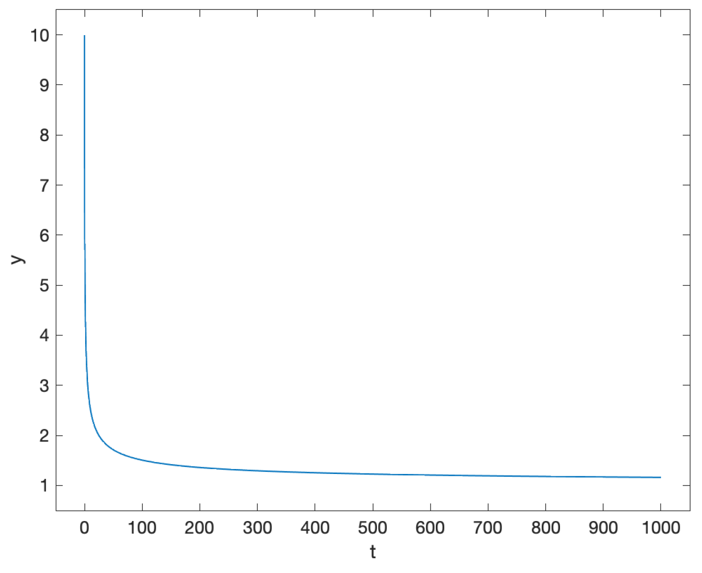
Figure 2.
Solution of Problem (39).
Figure 2.
Solution of Problem (39).
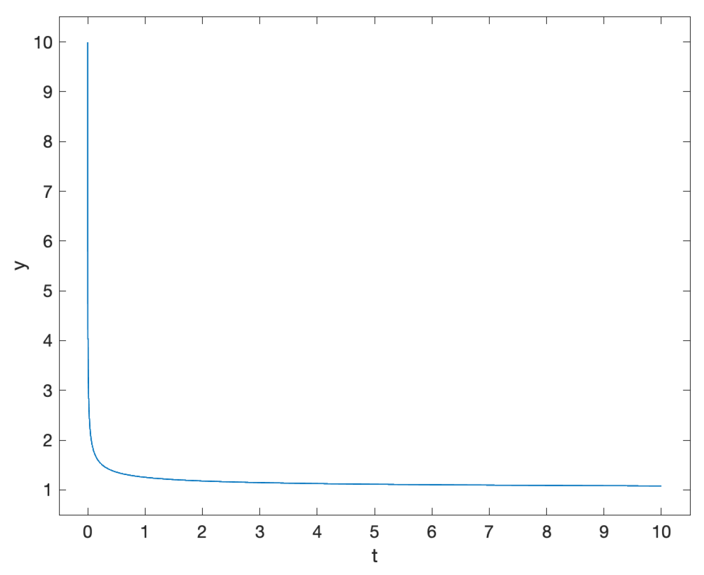
Figure 3.
Components of the solution of Problem (40).
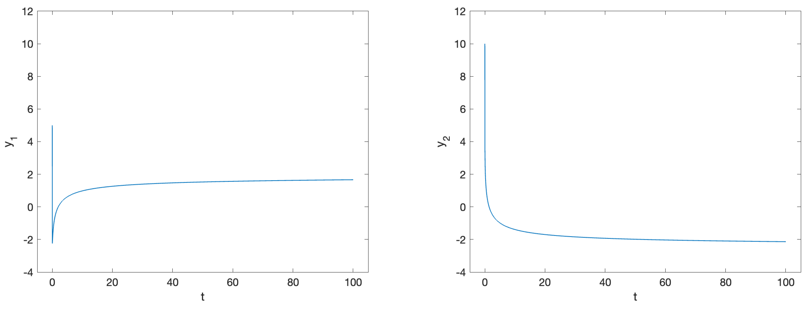
Figure 4.
Components of the solution of Problem (41).
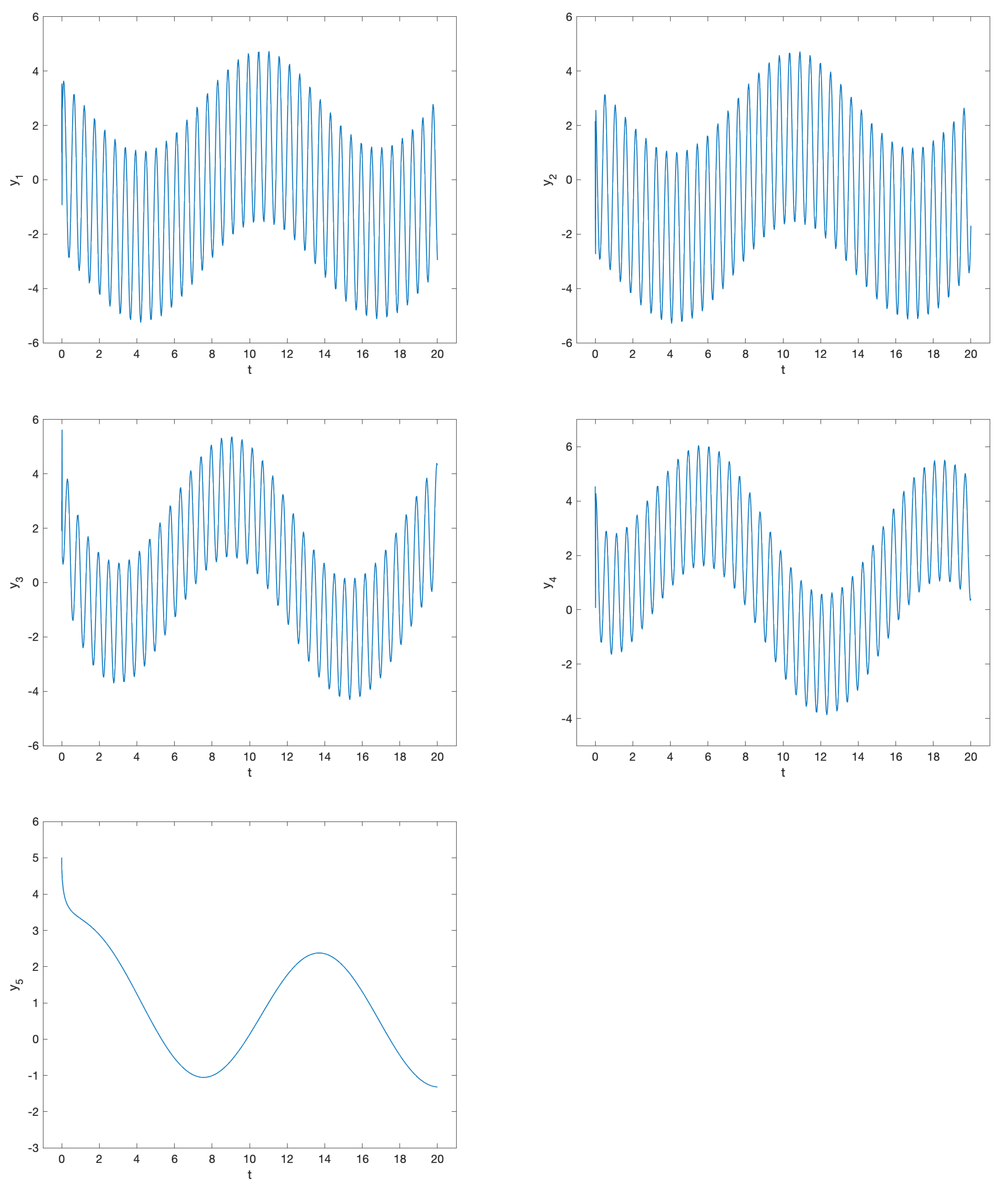
Figure 5.
Problem (42): solution (left-plot) and vector field (right-plot).
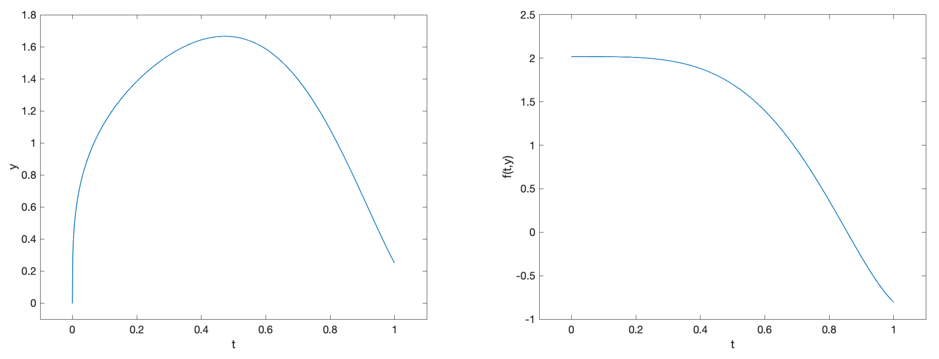
Figure 6.
Problem (43): solution (left-plot) and vector field (right-plot).
Figure 6.
Problem (43): solution (left-plot) and vector field (right-plot).

Figure 7.
Problem (44): solution (left-plot) and vector field (right-plot).
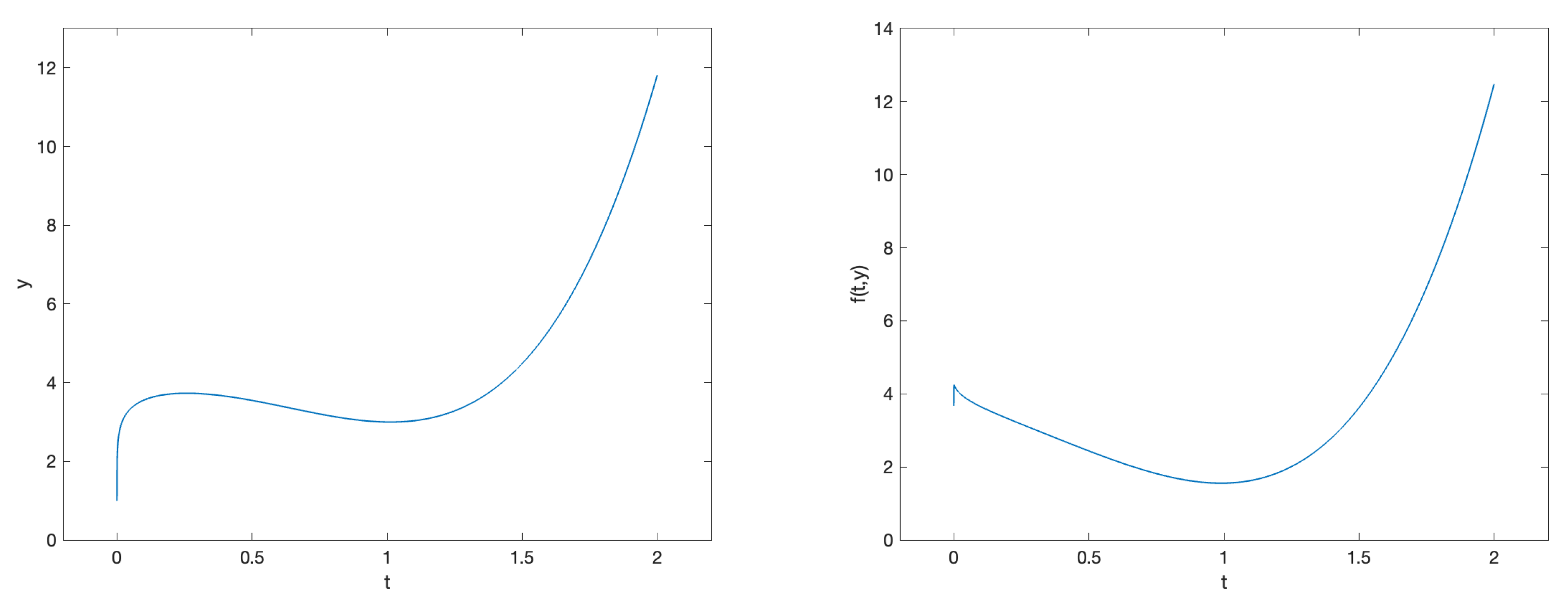
Figure 8.
Components of the solution of Problem (45).
Figure 8.
Components of the solution of Problem (45).
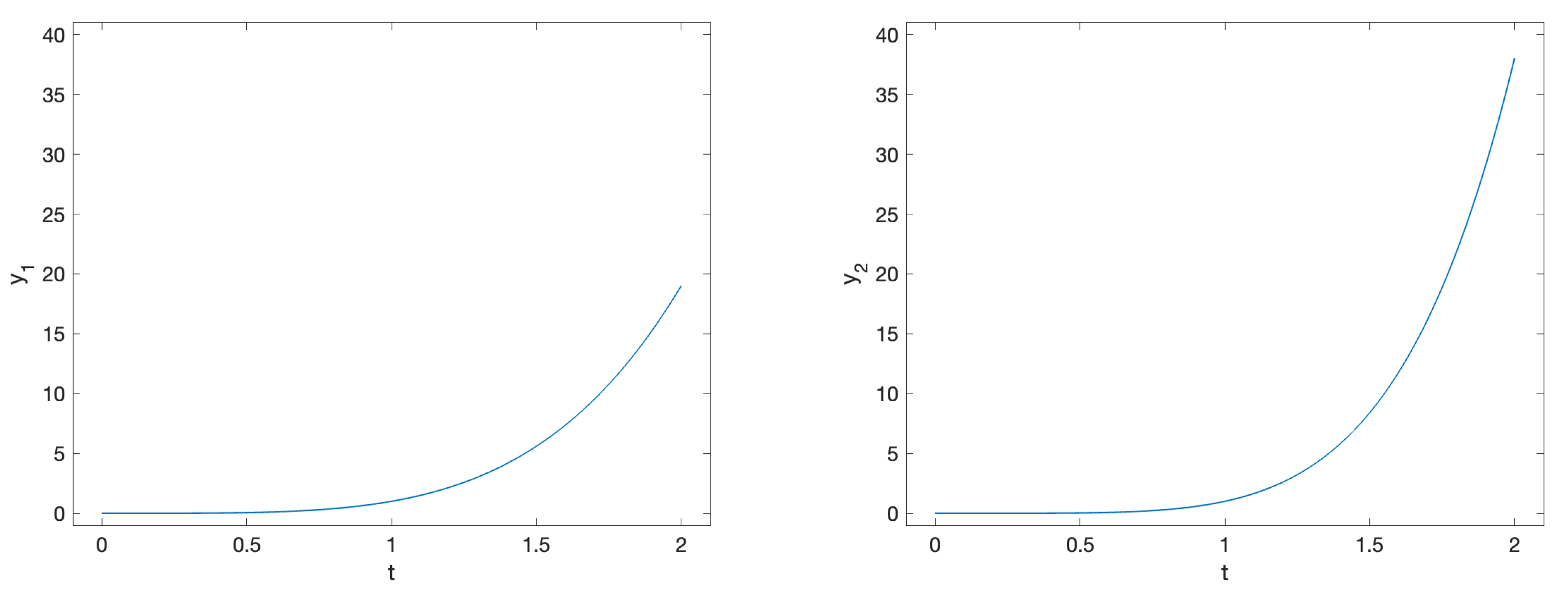
Figure 9.
Fractional Brusselator (46): solution in the phase space (left-plot) and plotted versus time (right-plot). In the left-plot, the red circle is the starting point of the trajectory.
Figure 9.
Fractional Brusselator (46): solution in the phase space (left-plot) and plotted versus time (right-plot). In the left-plot, the red circle is the starting point of the trajectory.
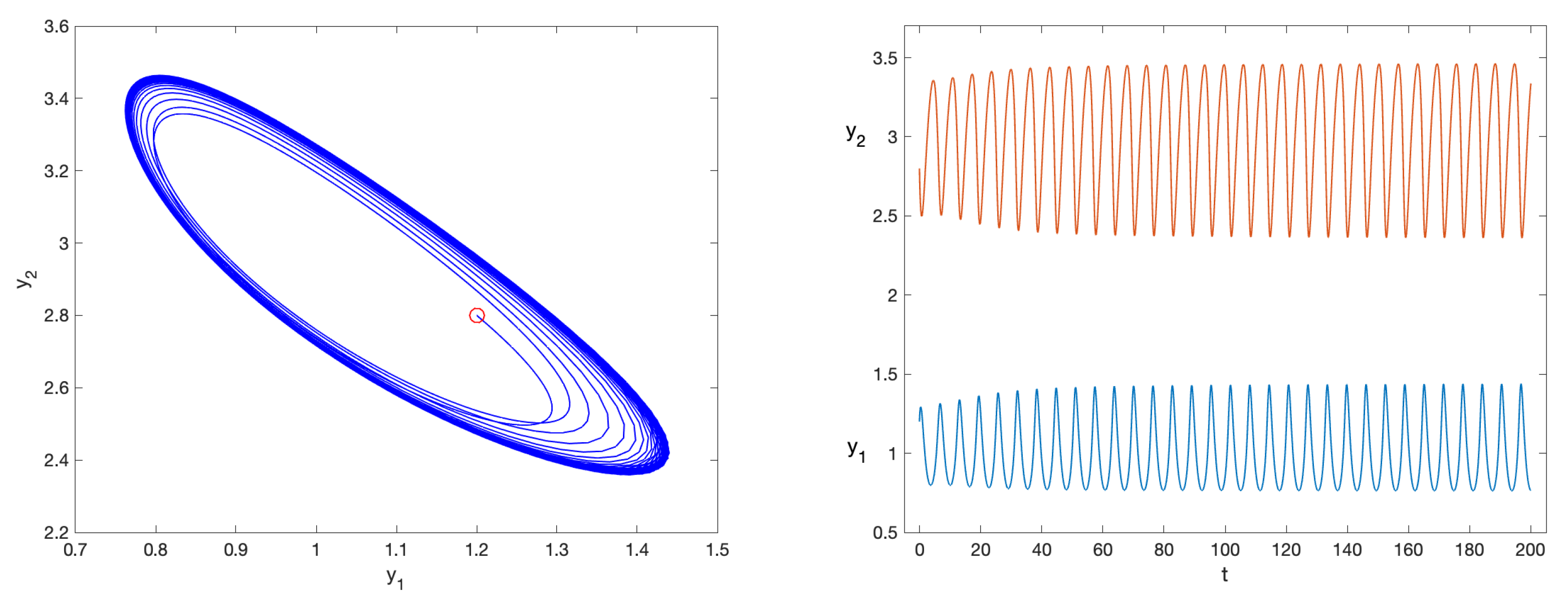
Figure 10.
Fractional Van der Pol problem (47): solution in the phase space (left-plot) and plotted versus time (right-plot). In the left-plot, the red circle is the starting point of the trajectory.
Figure 10.
Fractional Van der Pol problem (47): solution in the phase space (left-plot) and plotted versus time (right-plot). In the left-plot, the red circle is the starting point of the trajectory.
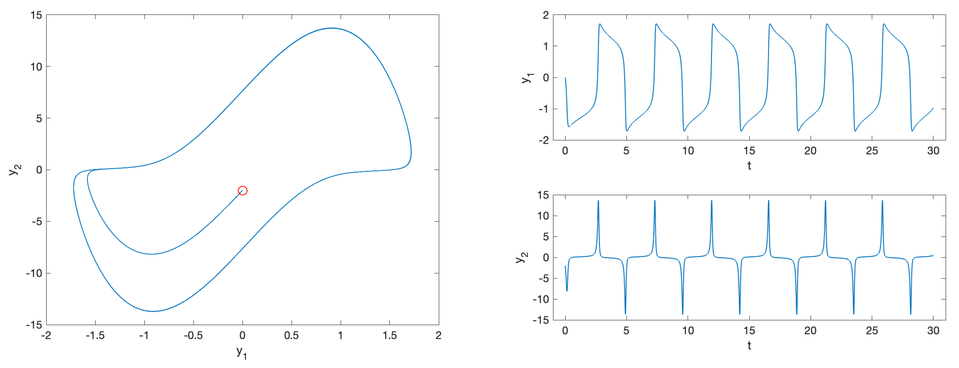
Figure 11.
WPD for Problem (38).
Figure 11.
WPD for Problem (38).
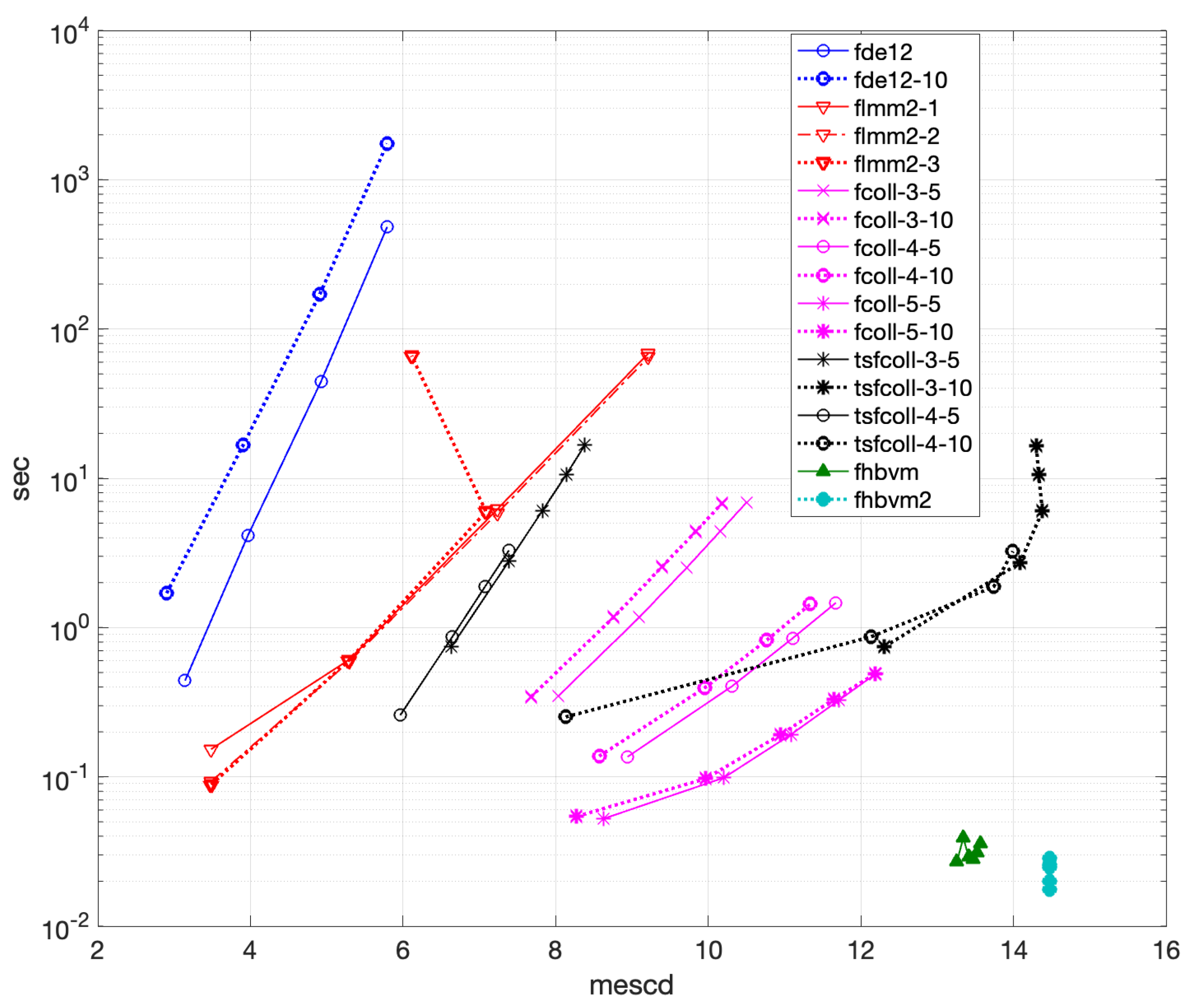
Figure 12.
WPD for Problem (39).
Figure 12.
WPD for Problem (39).
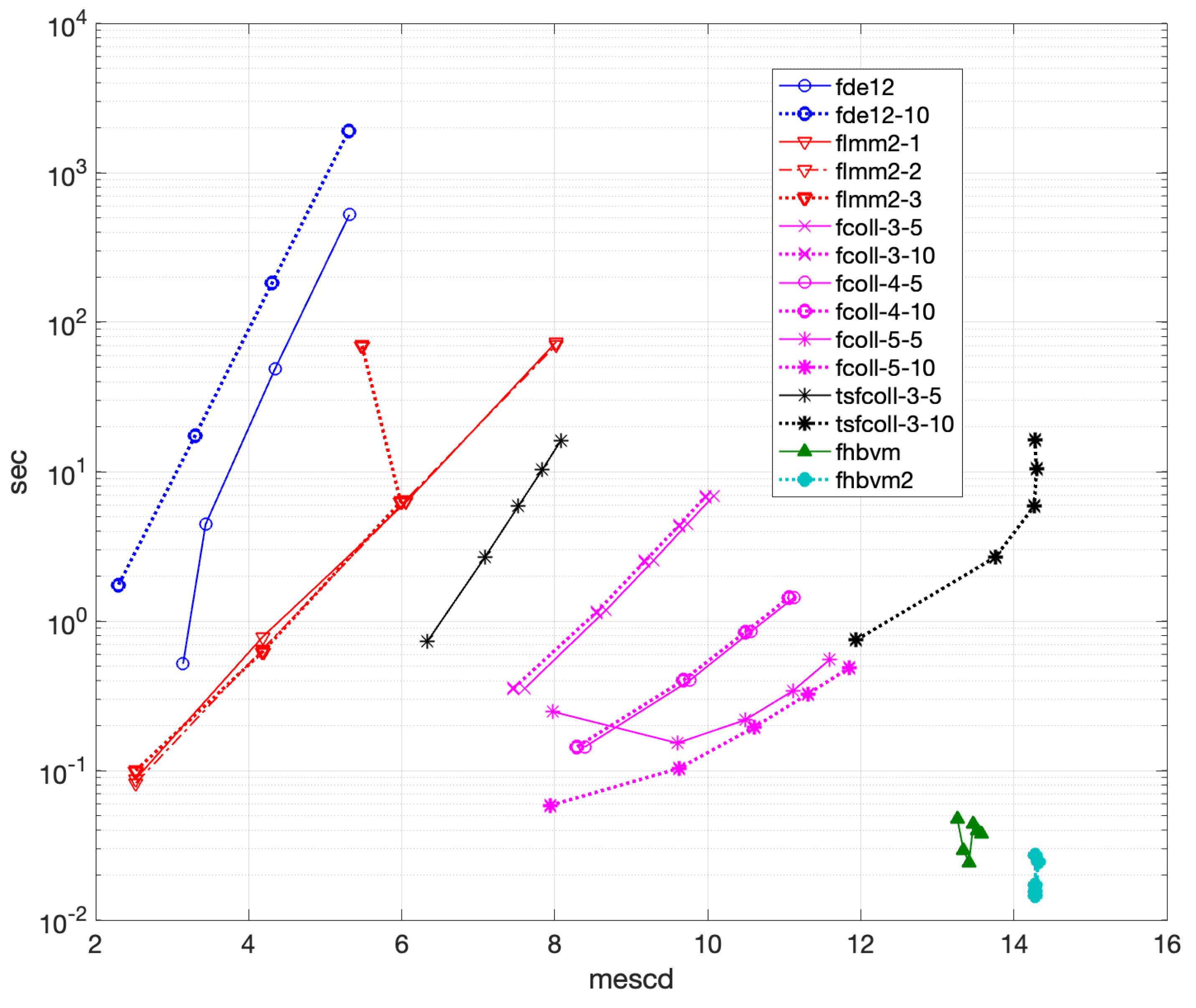
Figure 13.
WPD for Problem (40).
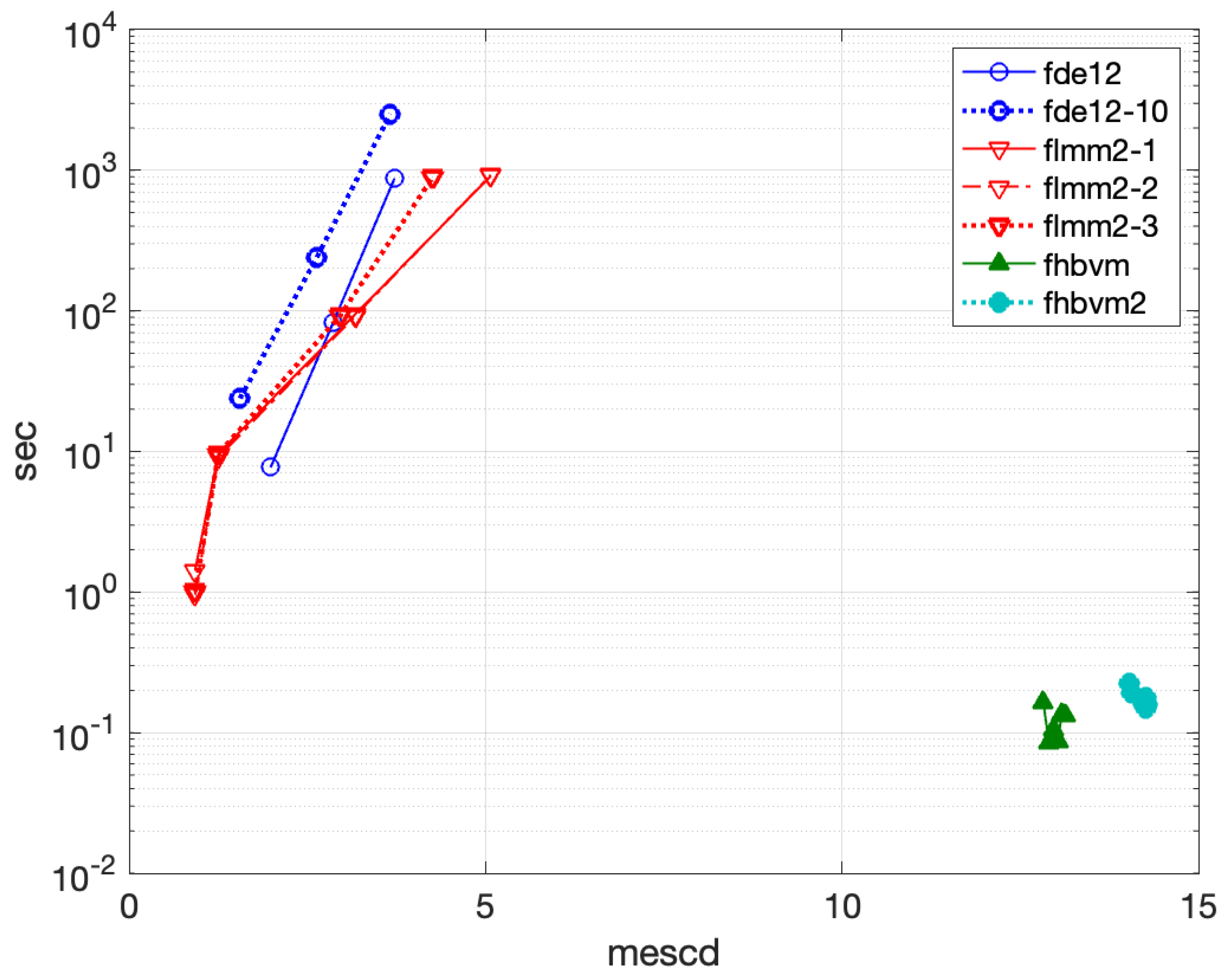
Figure 14.
WPD for Problem (41).
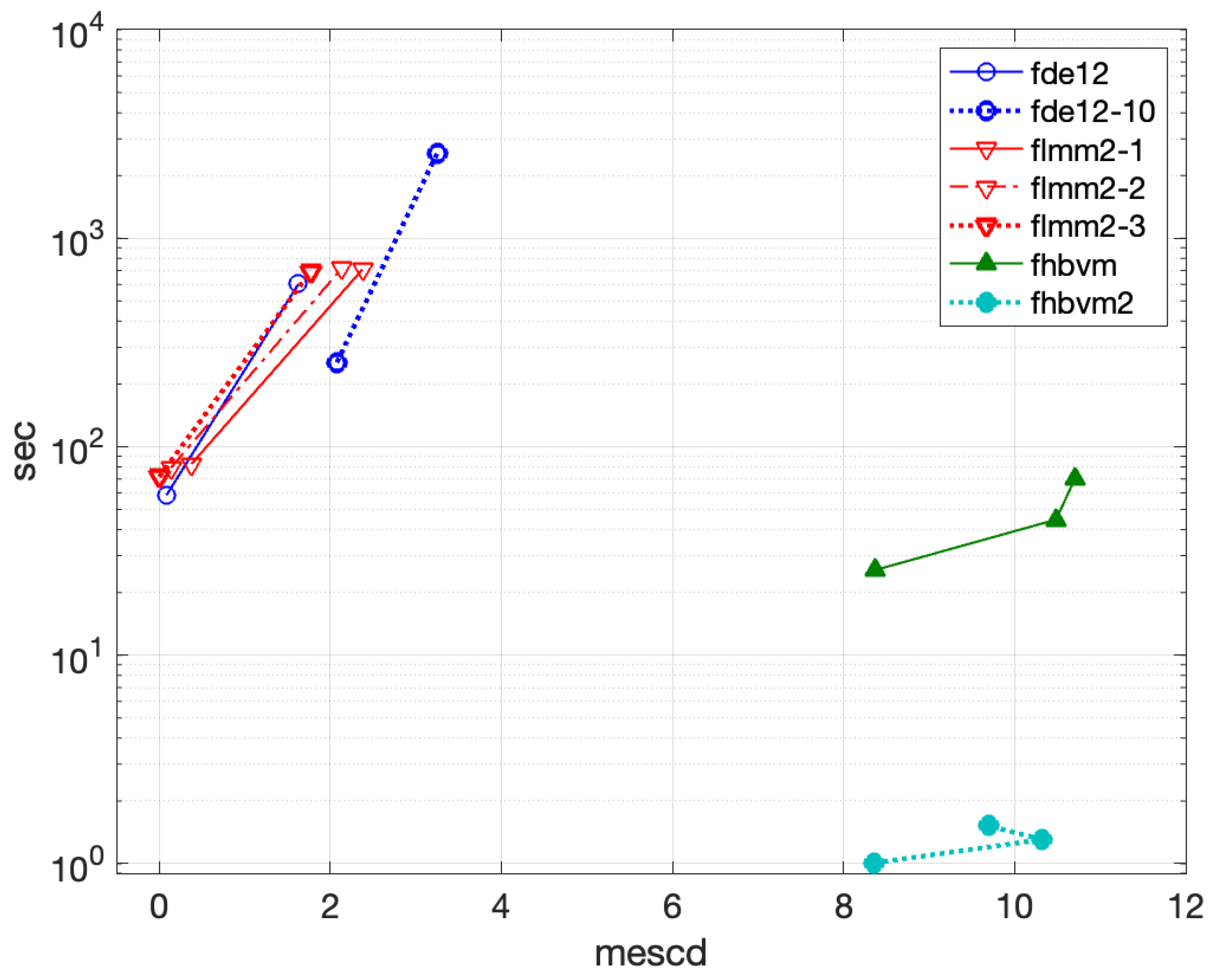
Figure 15.
WPD for Problem (42).
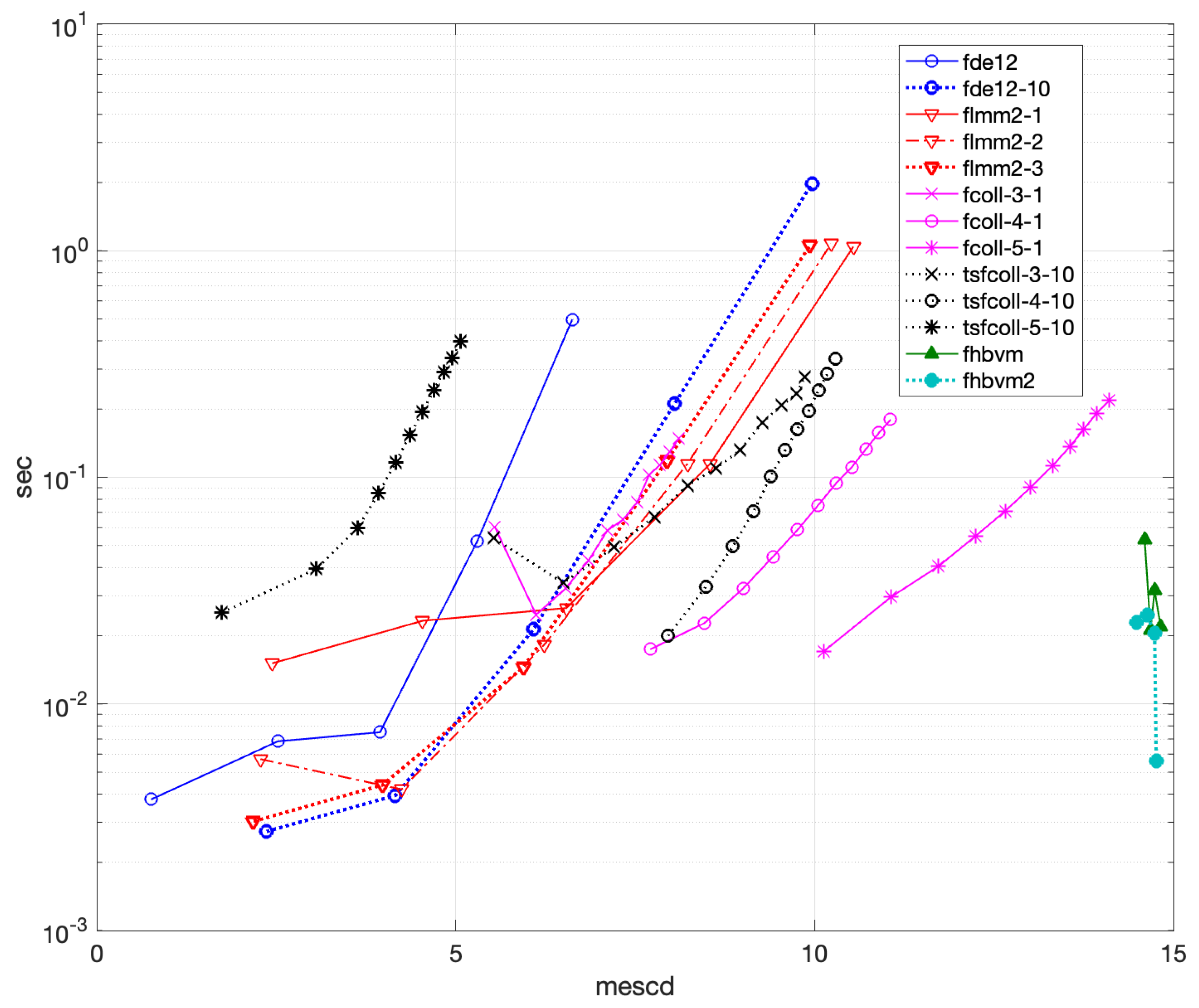
Figure 16.
WPD for Problem (43).
Figure 16.
WPD for Problem (43).
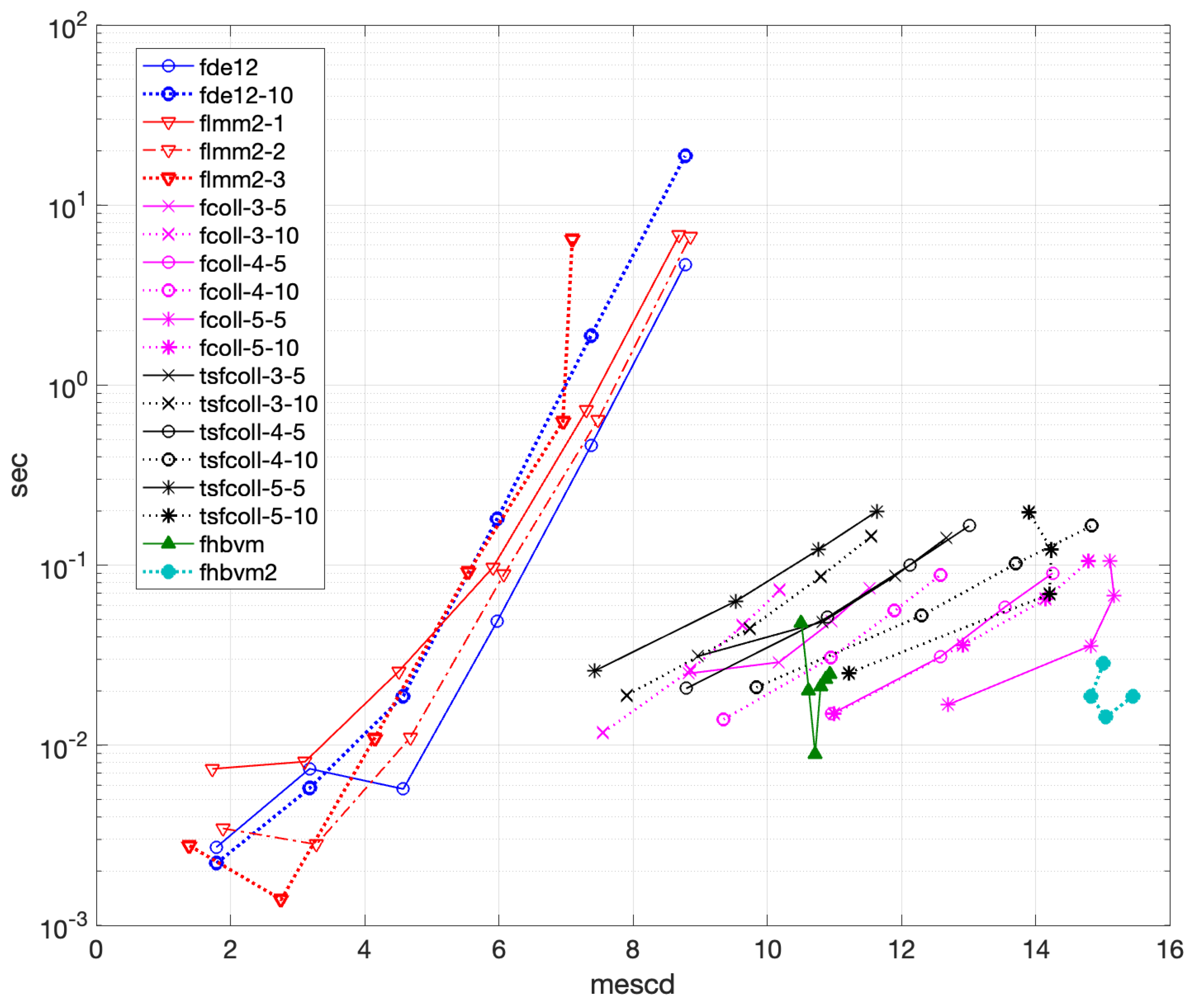
Figure 17.
WPD for Problem (44).
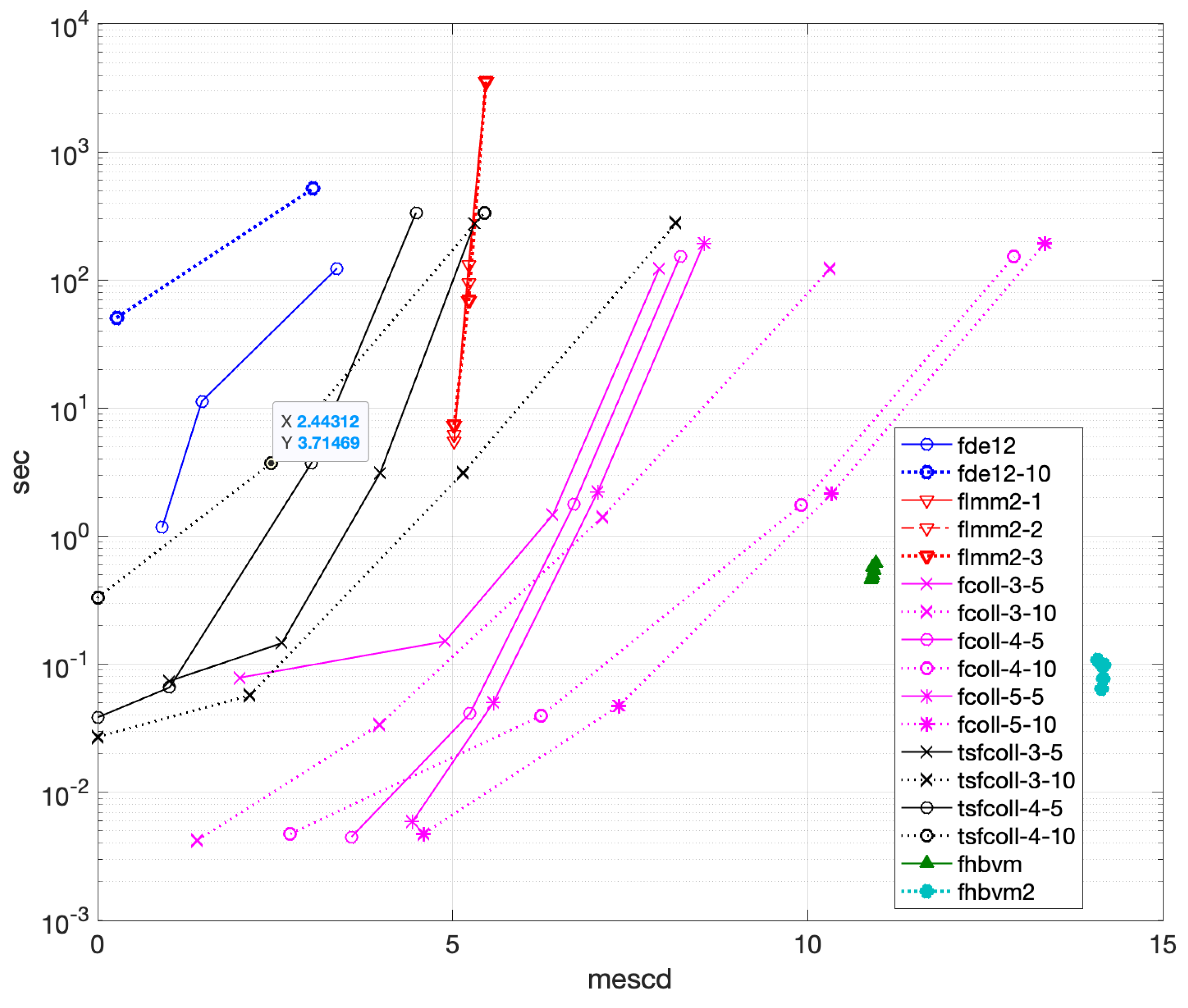
Figure 18.
WPD for Problem (45).
Figure 18.
WPD for Problem (45).
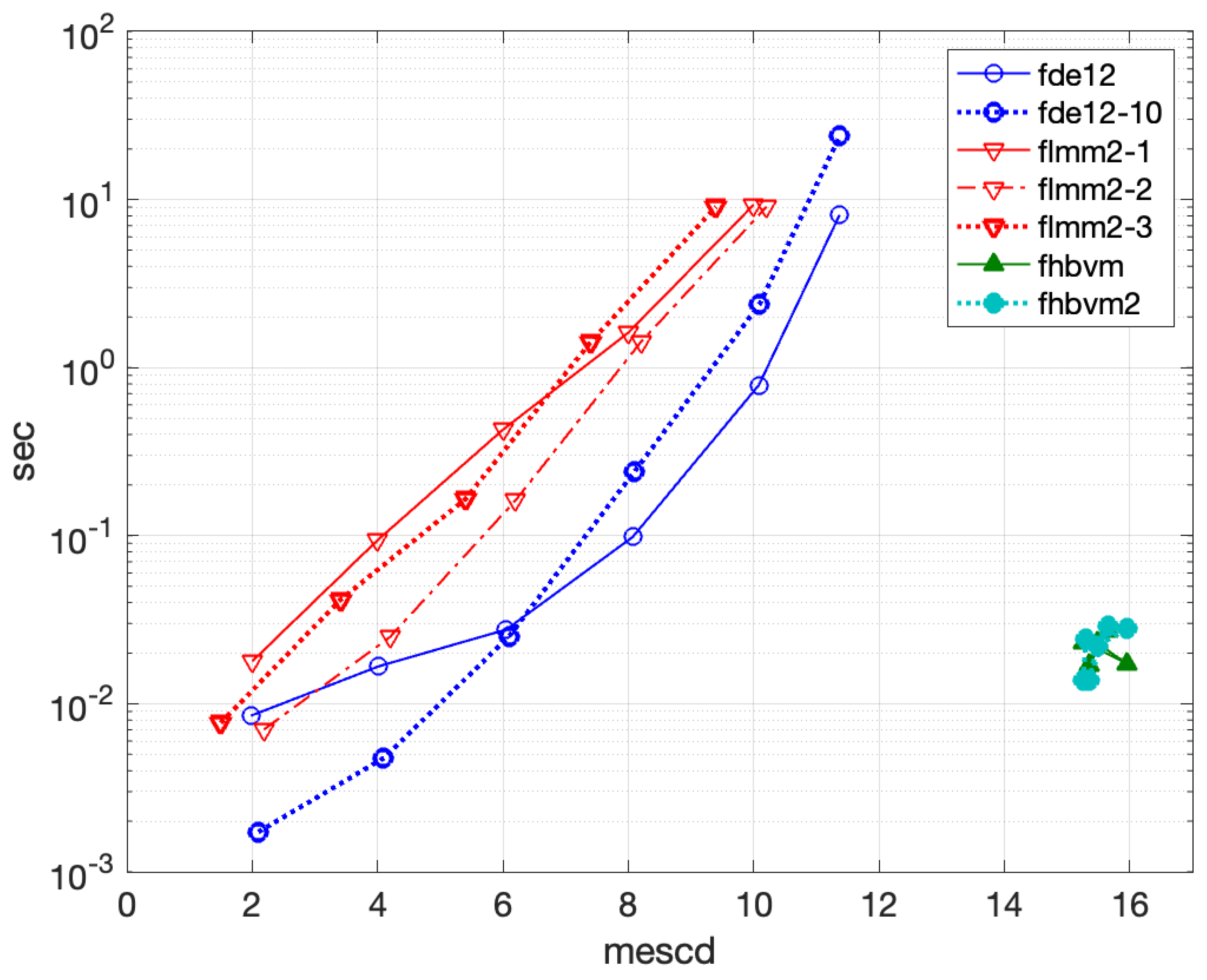
Figure 19.
WPD for Problem (46).
Figure 19.
WPD for Problem (46).
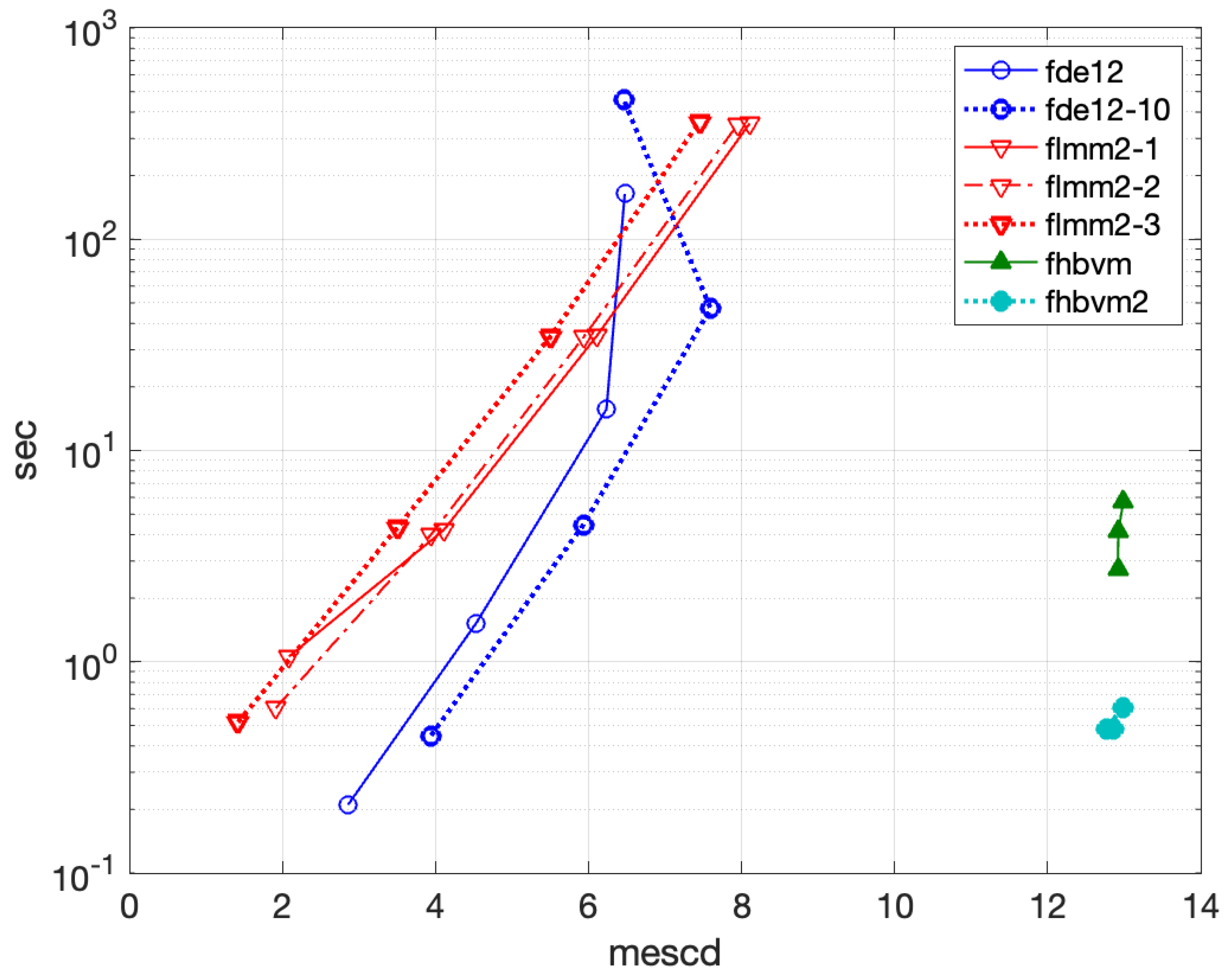
Figure 20.
WPD for Problem (47).
Figure 20.
WPD for Problem (47).
Disclaimer/Publisher’s Note: The statements, opinions and data contained in all publications are solely those of the individual author(s) and contributor(s) and not of MDPI and/or the editor(s). MDPI and/or the editor(s) disclaim responsibility for any injury to people or property resulting from any ideas, methods, instructions or products referred to in the content. |
© 2025 by the authors. Licensee MDPI, Basel, Switzerland. This article is an open access article distributed under the terms and conditions of the Creative Commons Attribution (CC BY) license (http://creativecommons.org/licenses/by/4.0/).
Copyright: This open access article is published under a Creative Commons CC BY 4.0 license, which permit the free download, distribution, and reuse, provided that the author and preprint are cited in any reuse.


