
Submitted:
03 April 2025
Posted:
04 April 2025
You are already at the latest version
Abstract
The finite volume method approach in computational fluid dynamics to numerically model a fluid flow problem involves the process of formulating the numerical flux at the faces of the control volume. This process is important in deciding the resolution of the numerical solution, thus its quality. In the current work, the performance of different flux construction methods when solving the one-dimensional Euler equations for an inviscid flow is analyzed through a test problem in the literature having an exact (analytical) solution, which is the Sod problem. The considered flux methods are: exact Riemann solver (Godunov), Roe, Kurganov-Noelle-Petrova, Kurganov and Tadmor, Steger and Warming flux-vector splitting, van Leer flux-vector splitting, AUSM, AUSM+, AUSM+-up, AUFS, five variants of the Harten-Lax-van Leer (HLL) family, and corresponding five variants of the Harten-Lax-van Leer-Contact (HLLC) family, Lax-Friedrichs (Lax), and Rusanov. The methods of exact Riemann solver and van Leer showed excellent performance. The Riemann exact method took the longest runtime, but the spread of runtime among all methods was not large.
Keywords:
Sod
; Shock tube
; Riemann problem
; Flux
; Euler
; MUSCL
1. Introduction
The term Riemann problem (Riemann, 1860; Castro-Orgaz and Hager, 2019) in basic gasdynamics refers to a setting where two adjacent regions of a compressible gas are initially separated by some barrier. Each region has a uniform set of conditions: density, velocity, and pressure. Suddenly, the barrier is removed and the energy imbalance between the two sides causes three waves such that some equilibrium average condition is encouraged. These waves can be a shock wave (normal shock), a contact discontinuity (contact surface), or an expansion fan (rarefaction fan). It is possible to have two shocks with no fans, two fans with no shocks, and one shock and one fan. In either case, a contact discontinuity would be separating the two other waves. There is also a possibility of reaching a vacuum state in zone surrounded by two contacts (one to the left and one to the right), which in turn separate two fans running away from each other (Kamm, 2015). However, the presence of vacuum is excluded in our work.
The simple Riemann problem is governed by the Euler equations (a system of time-dependent nonlinear hyperbolic partial differential equations), which admit discontinuities in the solution. For a computational fluid dynamics (CFD) solver built on the finite volume method (FVM) that is designed to handle compressible flows, the Riemann problem can be a good environment for testing the capability of the solver in forming fluxes at the finite volume face. The problem is focused on the convective/pressure flux in the one-dimensional space, thus eliminating complications of multi-dimensionality, inaccuracy of representing non-uniform boundary or initial conditions, and interference from other phenomena such as viscous effects and boundary layers, chemical reaction, mixing, multi-phase flow, heat transfer, thermal radiation, and source terms.
While the Riemann problem can be extended to more complicated environments (Hantke et al., 2020), the aim of this work is to solve a particular example of the basic Riemann problem known as the Sod problem with different numerical methods for building a flux vector at an cell interfaces, and analyze the results in comparison to the exact solution as well as to other numerical flux methods.
2. One-Dimensional Euler Equations
Euler formulation of a fluid motion neglects friction (viscosity) effects completely (Fletcher, 1991), leading to a reduced form of the Navier-Stokes equations. While Euler formulation may appear narrowly-restricted, there are many conditions where the effect of fluid viscosity can be safely neglected and this simplified formulation becomes accurate enough.
In vector form, the one-dimensional Euler equations governing inviscid fluids is (Hoffmann and Chiang, 1993)
where is a vector of the conserved variables, and is a vector of flux (sum of convective flux in the x-direction and a pressure contribution).
In the above equation, is the fluid density, which is the mass per unit volume; is the fluid velocity, so is the momentum per unit volume; is the total specific internal energy, so is the total internal energy per unit volume. The density , velocity , and pressure are referred to as the primitive variables.
The total specific internal energy is the specific internal energy plus the kinetic energy per unit mass, thus
The flux vector is
where is the total specific enthalpy
The specific enthalpy is
For a thermally perfect gas, the pressure, density, and absolute temperature are related as
where is the specific gas constant. Also, for a thermally perfect gas, the specific heat capacity at constant volume and the specific heat capacity at constant pressure both vary with the temperature only, and the following relation holds true:
The ratio of the specific heat capacities , also called the adiabatic index, is
The following equations apply to a thermally perfect gas
where is the speed of sound in the gas (the sonic speed), and is the Mach number. If a thermally perfect gas has also the specialty that its specific enthalpy and its specific internal energy can be related as
with being now a constant independent of the temperature, then the gas is described as calorically perfect and its specific heat capacities are also independent of the temperature (Fletcher, 2004). The calorically perfect gas assumption is usually reasonable for compressible flows at low speeds. This simplification permits analytical analysis for supersonic flows (NACA, 1953).
For a calorically perfect gas, the following formulas apply
This work considers a calorically perfect gas that is non-reacting and inviscid.
3. Sod’s Problem
A shock tube is a special case of the Riemann problem, in which the compressible gas on either side is initially stationary (Laney, 1998). Figure 1 gives a graphical illustration of the Riemann problem at the initial state. The Sod problem (Sod, 1978) is a shock tube problem with certain initial left and right densities and pressures, causing a right-going shock wave, a left-going expansion fan, and a right-going contact discontinuity in between. Table 1 contrasts the left and right conditions in the Sod problem at the initial state . The initial distribution of the primitive variables is demonstrated in Figure 2. The jump is located at a position , which is midway between the left end of the problem domain and its right end . Table 2 gives a summary of the fan-contact-shock wave pattern in the exact solution of the Sod problem.
At a time of , the exact solution we obtained for the Sod problem is illustrated in Figure 3, expressed in terms of the primitive variables and the Mach number. The abrupt change in the pressure designates the location of a shock wave traveling to the right. The abrupt change in the density where no other variable showing any change designates the location of a contact discontinuity, which also travels to the right. The gradual change in all the variables designates the extent of an expansion fan, which travels to the left. The left front of the fan is called the head, and the right edge is called the tail.
4. Validation
The computation of the exact solution presented earlier in this work, as well as the numerical ones to be presented later, is done using computer codes written in GNU Octave, a scientific programming language (Eaton, 2020). As our exact solution is to be used as a reference for judging numerical ones, it is important to check its validity. This is supported here in two ways.
The first validity support of our implementation of the exact Riemann solver is through satisfying the Rankine-Hugoniot shock condition (Rankine 1870; Hugoniot 1887, 1889; Koval and Szabo, 2008) for the mass. The condition is used to compute a shock speed other than the one obtained from the exact Riemann solver (was given already in Table 2) as
where the operator represents the difference across the shock wave. This speed matches the one given earlier in Table 2, which was found independently as
where , , and are the gas velocity, speed of sound, and pressure in the right undisturbed state; and is the pressure around the contact discontinuity.
The second validity support of the provided exact solution of the Sod problem is through comparison with published exact and computational solutions at the same time taken from the Castro project validation data (Castro, 2020). Figure 5 shows these published results for the primitive variables. Visual inspection suggests they match with our solution given in Figure 3.
5. Face Flux Construction
The time integration of the conserved variables is done using Godunov scheme (Godunov, 1959), which is a conservative explicit finite volume formula. For a uniformly spaced one-dimensional array of computational cells having a cell width of , let the cell center positon index be , then the left face flux vector is and the right face flux vector is . Time integration of the conserved variables vector over one time step is done as
The time index refers to the latest known variable values, while the index refers to the new values after time integration over one time step. The scheme is explicit, where the updating of a cell value is independent of updating other cells. This eliminates the need for solving a system of algebraic equations. Godunov scheme is of first order accuracy in time. The spatial accuracy depends on how the face flux vectors are constructed. It can be first order (lowest resolution) or second order (higher resolution).
Godunov scheme appears simple and straightforward, provided that the face flux vectors have been computed and are made available to the scheme.
The process of preparing face flux vectors at intercell faces is split into two steps:
- Step 1 (MUSCL): use neighbor cell-center values of the primitive variables to extrapolate and/or interpolate a ‘fictitious’ value at both sides of the facial interface. The left side of the face has the values denoted by: . These are the locally left values. Similarly, the right values of the face are denoted by: . These are the locally right values. It should be noted that although physically these locally left and locally right values are defined at the same spatial location, they are not necessarily equal. Once these fictitious face-left and face-right values are computed, a local fictitious Riemann problem is constructed. There is a jump in one or more flow variables across the face. Along with the interpolation/extrapolation, the preparation of the local Riemann problem at each face includes also the use of flux limiters (also called slope limiters) through a scheme called MUSCL, which stands for Monotonic Upstream-centered Scheme for Conservation Laws (van Leer, 1979). This scheme is a nonlinearized version of the so-called 3-point scheme of parabolic interpolation/extrapolation (Waterson and Deconinck, 2007). Whereas the interpolation/extrapolation coefficients in the scheme are solution-independent, the MUSCL scheme adds to the scheme a solution-dependent limiter, which downgrades the interpolation/extrapolation level near sharp changes (like a shock wave) to use only the nearest cell-center value, while upgrades it to allow use of more cell-center values in regions of smooth variations. This adaptive switching allows the use of the high-resolution with its advantage of spatial accuracy without suffering from severe oscillations near sharp changes by ‘switching off’ the high-resolution capability and keeping only the first-order spatial accuracy. There are different flux limiters (Chu and Gao, 2013; Li et al., 2020). We here use the van Leer flux limiter (van Leer, 1974), which has intermediate characteristics among others in terms of the dissipation level (Bai et al., 2018).
- Step 2 (flux method): After a local fictitious Riemann problem is constructed, then comes the step of inferring a face flux vector based on the jump across the local left and local right flow variables. This step is the core of this work. We here consider 22 methods of face flux methods proposed in the literature, and compare their performance for the Sod problem as a test case.
To explain the MUSCL step, consider a generic variable that has a value in four adjacent cell centers as shown in Figure 4. The cell values are labeled in the direction of the increasing x-coordinate as . The goal is to construct a limited interpolated/extrapolated fictitious left and right values at the face separating the cell and the cell .
Let
Two consecutive gradient ratios are calculated, left one and right one, respectively, as
There is a possibility of a division by zero when calculating and . However, this is avoided by applying the following condition
where is a small threshold, which was decided by the computing program as .
Then, two flux limiting values and are obtained for the left and right sides of the face, respectively, using the van Leer flux limiter function.
Now, the final stage is to compute the fictitious left and right face values and , respectively, using the following version of the MUSCL scheme:
In the case of unity flux limiters , the above equations represent a pseudo linear-upwind interpolation (LUI), which is also called second order upwind (SOU). In that case, each of the fictitious face value is constructed by a standard linear extrapolation from the two nearest cell-center values on the same face side (either left or right). This pure extrapolation (no interpolation) feature corresponds to setting the parameter value in the linear version of the MUSCL scheme (the scheme).
On the other hand, if the flux limiters are set to zero , then a pseudo first order (classical upwinding) interpolation is obtained, where each fictitious face value is simply taken as the nearest cell-center value on the same face side (either left or right). The term ‘pseudo’ is used in the above text because in true upwinding schemes, taking the left or right cell-center values depends on the speed of the characteristic (Strikwerda, 2004), also called the wave speed or the information speed, relevant to the concerned variable at the face. Such checking of the direction of the information is not done here, and it is always assumed that for the left fictitious face value, the flow information (the wind) comes from the left, and for the right fictitious face value, it comes from the right.
6. Analyzed Flux Methods
Twenty two flux methods are tested in this work and they are listed here with a brief description on each. Giving detailed explanation or the mathematical formulation behind each method can make this section extremely long. Instead, the interested reader is cordially requested to visit the literature for deeper information about any of methods found of interest. In presenting the data, a short name (a code) is assigned to each method as a quick unique identifier. The methods are listed below by their codes. The sequence of introducing the methods here is the same one used later when presenting their graphical results and the detailed root-mean-square errors of their numerical results.
6.1. Riemann
This flux method is also called Godunov solver. Godunov is credited to formulate this exact (analytic) Riemann solver in the same reference cited before when addressing the Godunov time integration scheme. This flux method solves a Riemann problem exactly at each intercell face, with the local fictitious face-left and face-right conditions provided by the MUSCL scheme replacing the global initial physical left and right states of the gas in the Sod problem. This local Riemann solver identifies the state of the gas at the face interface, such as a zone between a left-going expansion fan and a right-going contact discontinuity, or a zone between a right-going shock wave and a right-going contact discontinuity, or a zone within an expansion fan whose tail and head go opposite to each other, which is called a transonic fan as it accelerates the gas from subsonic (Mach number < 1) to supersonic (Mach number > 1). Then, the face flux is constructed using the primitive values of the identified state. Thus, if the identified state has numerical values of the density, velocity, and pressure denoted by , then the constructed face flux is simply
6.2. Roe
This is the Roe approximate solver for face flux, which is also known as Roe upwind scheme (Roe, 1981). The nonlinear flux vector in Euler equations is replaced by a locally linearized approximate flux function, which utilizes matrix called a Roe-average Jacobian matrix. Roe flux method gives three equally-spaced waves. It cannot capture the spread of the expansion fan. Instead, it represents it as a zero-thickness wave. Denote the MUSCL returned face-left values of the density and velocity by and , respectively; and the MUSCL returned face-right values of the density and velocity by and , respectively. Then, Roe method introduces a customized square-root-density-weighted velocity defined as: . A face-left specific total enthalpy is , where is the face-left pressure as provided by the MUSCL scheme. Similarly, a face-right specific total enthalpy is , where is the face-right pressure as provided by the MUSCL scheme. The Roe method introduces a square-root-density-weighted total specific enthalpy defined as: . Finally, a Roe-specific speed of sound is defined as: . The three wave speeds in Roe method (also called Roe eigenvalues) are: The three Roe specific quantities (, , and ) are used to construct the face flux vector.
6.3. KNP
This is the central-upwind method of Kurganov, Noelle, and Petrova for the face flux (Kurganov at al., 2001). The term central-upwind here comes from the notice that the method is central in principle (thereby, offering high resolution with small dissipation), but still has an upwinding character by respecting the direction of the wave travel. The method does not attempt to approximate the exact flux as in the case of Roe method.
6.4. KT
This is another central-upwind method by Kurganov and Tadmor for forming the intercell face flux vector (Kurganov and Tadmor, 2000). It resembles the KNP method in structure, with the KT method (which is chronologically earlier) being simpler. For example, the KT method assigns fixed weights of 0.5 to the face-left and face-right MUSCL flux vectors, whereas the KNP method uses flow-based weights.
6.5. SW
This is the Steger and Warming flux-vector splitting (FVS) method for face flux (Steger and Steger, 1979 and 1981). The face flux vector is computed as a sum of two flux vector: a plus one and a minus one, as . The subvector is associated with the positive eigenvalues of the Jacobian matrix , while the subvector is associated with its negative eigenvalue es.
6.6. vanLeer
This is another flux vector splitting (FVS) method, made by van Leer (van Leer, 1982). It allows continuous slope of two formulation functions at the special values of Mach numbers -1, 0, and 1. A quadratic function of the fictitious face-left and face-right Mach numbers are introduced. This addresses a shortcoming in the in the chronologically earlier SW flux vector splitting method.
6.7. AUSM
This is the Advection Upstream Splitting Method (AUSM) for face flux construction (Liou and Steffen, 1993). The flux is divided into a pressure component and a convective component for better treatment.
6.8. AUSM+
This is a follow-up improvement (Liou, 1996) of the Advection Upstream Splitting Method (AUSM) for computing face fluxes by addressing observed shortcomings in some cases in which the original AUSM technique did not maintain its tradition of accuracy and efficiency.
6.9. AUSM+-up (for All Speeds)
It is an extension of AUSM+ to have the convergence rate nearly independent of the Mach number for the low-Mach subsonic limit up to a freestream Mach number of 0.5. This is achieved through proper scaling using asymptotic analysis (Liou, 2006). Also the convergence rate is nearly constant in transonic and supersonic flows.
6.10. AUFS
AUFS stands for Artificially Upstream Flux Vector Splitting method (Sun and Takayama, 2003). It employs two simultaneous flux-vector splitting mechanisms, one by dividing into pressure and non-pressure components, and another by using a method-specific Mach number (one that is based on the simple average of the face-left and face-right velocities, ) as a splitting weight. The method also respects the sign of the average velocity of the face-left and face-right fictitious values. The method is relatively easy to implement.
6.11. HLL-Davis1
This is the Harten, Lax, van Leer (HLL) 2-wave model (Harten et al., 1983), with Davis first estimation of right and left wave speeds (Davis, 1988). Let , , and be the face-left fictitious values of the density, velocity, and pressure, respectively; and , , and be their face-right counterparts. Then, a face-left speed of sound is calculated as , and face-right speed of sound is calculated as . This version of the HLL family of methods sets the left wave speed as , and the right wave speed as .
6.12. HLL-Davis2
This is a second variant of the Harten, Lax, van Leer (HLL) 2-wave model, with Davis second estimation of right and left wave speeds. With the same meaning of as used in the HLL-Davis1 method earlier, this other version of the HLL family sets the left wave speed as , and the right wave speed as . The function returns the smaller of the two arguments, and the function returns the larger of them.
6.13. HLL-Roe
This is a third variant of the Harten, Lax, van Leer (HLL) 2-wave model, with two of the Roe eigenvalues used for the right and left wave speeds. Using same notations in the Roe method and the HLL-Davis1 method, the two wave speeds in the HLL-Roe method described here are: and .
6.14. HLL-Einfelt
This is a fourth variant of the Harten, Lax, van Leer (HLL) 2-wave model, with Einfelt eigenvalues for the right and left wave speeds (Einfeldt, 1988). It is also called (HLLE) flux method. The left and right wave speeds here are: and , respectively. The symbol refers to the Roe square-root-density-averaged velocity as described in the Roe method. The velocity is computed as: . A subscript refers to a face-left value, and a subscript refers to a face-right value. The face-left speed of sound and the face-right speed of sound are as discussed in the HLL-Davis1 method.
6.15. HLL-pBased
This is a fifth variant of the Harten, Lax, van Leer (HLL) 2-wave model, with pressure-based calculation for right and left wave speeds (Toro et al., 1994). The method introduces a customized threshold or criterion pressure used to determine the left and right wave speeds, where . The left and right wave speeds here are: and , respectively. The symbols in these formulas have the same meanings as those given for the HLL-Davis1 method. Two new symbols appear here ( and ), which are factors decided based on and how it compares with the face-left pressure and the face-right pressure , as follows: if , if , if , and if .
6.16. HLLC-Davis1
This is an extended 3-wave version (Toro et al., 1992) of the Harten, Lax, van Leer, Davis (HLL-Davis1) 2-wave model, where a third wave (contact discontinuity or contact surface) is included. The additional "C" letter in the method code stands for the added "contact" wave. This method for flux construction is comparable in accuracy and robustness to that of the exact Riemann flux method, while being simpler and computationally less demanding than it. Davis first estimation of right and left wave speeds is used.
6.17. HLLC-Davis2
This is an extended 3-wave version of the Harten, Lax, van Leer, Davis (HLL-Davis2) 2-wave model, where a third wave (contact discontinuity) is added.
6.18. HLLC-Roe
This is an extended 3-wave version of the Harten, Lax, van Leer, Roe (HLL-Roe) 2-wave flux model, where a third wave (contact discontinuity) is added.
6.19. HLLC-Einfelt
This is an extended 3-wave version of the Harten, Lax, van Leer, Einfelt (HLL-Einfelt or HLLE) 2-wave flux model, where a third wave (contact discontinuity) is added.
6.20. HLLC-pBased
This is an extended 3-wave version of the Harten, Lax, van Leer, pressure-based (HLL-pBased) 2-wave flux model, where a third wave (contact discontinuity) is added.
6.21. LF
The Lax-Friedrichs (LF) method, which is also called the Lax method (Lax, 1954) is a basic explicit three-point technique used for solving time-dependent partial differential equations. It is first-order accurate in space. This method gives the most dissipative flux among all basic stable explicit flux construction methods. The method does not require solving a Riemann problem (either exact or approximate) at each cell face. The face flux is constructed as , where and are the flux vector after substituting with the face-left and face-right values of the primitive variables, respectively; and are the conserved variables vectors after substituting with the face-left and face-right values of the primitive variables, respectively; is the cell width (the spatial step); and is the time step.
6.22. Rusanov
This is a single-wave simplification of Roe 3-wave model (Rusanov, 1970). It is also called generalized Lax-Friedrichs flux method. Like the Lax-Friedrichs flux method, this method does not require solving a Riemann problem (either exact or approximate) at each cell face. However, unlike the Lax-Friedrichs flux method, it makes use of the local speed of sound. The flux calculation formula is nearly identical to the one given for the Lax-Friedrichs flux method, with the only difference is that the uniform virtual speed is replaced by a gas-dependent speed , where and are the absolute values of the face-left and face-right gas velocities, respectively; and and are the speeds of sounds obtained using the face-left and face-right densities and pressures, as mentioned for the HLL-Davis1 method.
7. Graphical Results
The Sod problem is solved numerically using each of the listed 22 flux methods in the previous section. No other change was done from one numerical simulation to another. Common simulation settings include a cell size of (thus, the shock tube of unit length is divided into 200 equal cells), and a time step of , which was related to the cell size as
where is the desired upper limit of the Courant number (Courant–Friedrichs–Lewy, CFL, number) as a condition for spatio-temporal stability in explicit time integration of partial differential equations, requiring the Courant number (Co) to be below unity. As the Co decreases, stabilizing numerical dissipation increases (Chang and Wang, 2003). The parameter is an estimate of the maximum wave speed in the problem. We set , which is a reasonable value for the highest possible sum of the local absolute gas velocity and the speed of sound in the problem, . The target maximum Courant number was set to . This target was largely satisfied in all performed 22 simulations, as found by post-processing the simulation results.
In Figures 6–27, two plots are assigned per figure, and each figure represents results using one of the flux methods. The order of presenting the graphical results of the flux methods is the same one used when briefly describing them earlier. The first plot in each figure is the spatial distribution of the three primitive variables (density , gas velocity , and pressure ) at the final simulation time of 0.2 (thus, after 200 time steps). The other plot in each figure shows the spatial distribution of the local Mach number (which is initially zero everywhere) at the final simulation time of 0.2. The title of each plot includes the code (the short name) of the flux method used in the simulation. In addition, the maximum observed Co number (CFL number) is also listed in the plots titles.
The LX method in Figure 26 shows significant undesirable dissipation causing severe smearing of jumps in the solution. No other method showed such level of unacceptable performance.
AUSM (Figure 12) exhibits a small overshoot at the tail of the fan. AUSM+ (Figure 13) did not resolve this problem, but it disappears in the further-improved version of AUSM+-up (Figure 14).
The flux methods of Roe, KT, SW, AUFS, HLL-Davis1, HLL-Roe, HLL-Einfelt, HLL-pBased, HLLC-Davis1, HLLC-Roe, HLLC-Einfelt, HLLC-pBased, and Rusanov show small velocity oscillations (wiggles) to the left of the shock (i.e., after the gas is shocked). These wiggles are particularly noticeable with the SW method.
The flux methods of the exact Riemann solver (Figure 6), KNP (Figure 8), vanLeer (Figure 11), AUSM+-up (Figure 14), HLL-Davis2 (Figure 17), and HLLC-Davis2 (Figure 22) appear to perform the best in terms of being free from visual oscillations in the solution.
Within the expansion fan, near its head, the methods of AUSM (Figure 12), AUSM+ (Figure 13), and AUFS (Figure 15) do not capture well the spatial increase of the gas velocity. They produce a fan head that is shifted to the right of its exact location. On the other hand, the methods of KT (Figure 9), SW (Figure 10), and vanLeer (Figure 11) satisfactorily predict the propagation of the fan head.
Figure 6.
Calculated final primitive variables and Mach number, using face flux of exact Riemann solver (also called Godunov flux).
Figure 6.
Calculated final primitive variables and Mach number, using face flux of exact Riemann solver (also called Godunov flux).
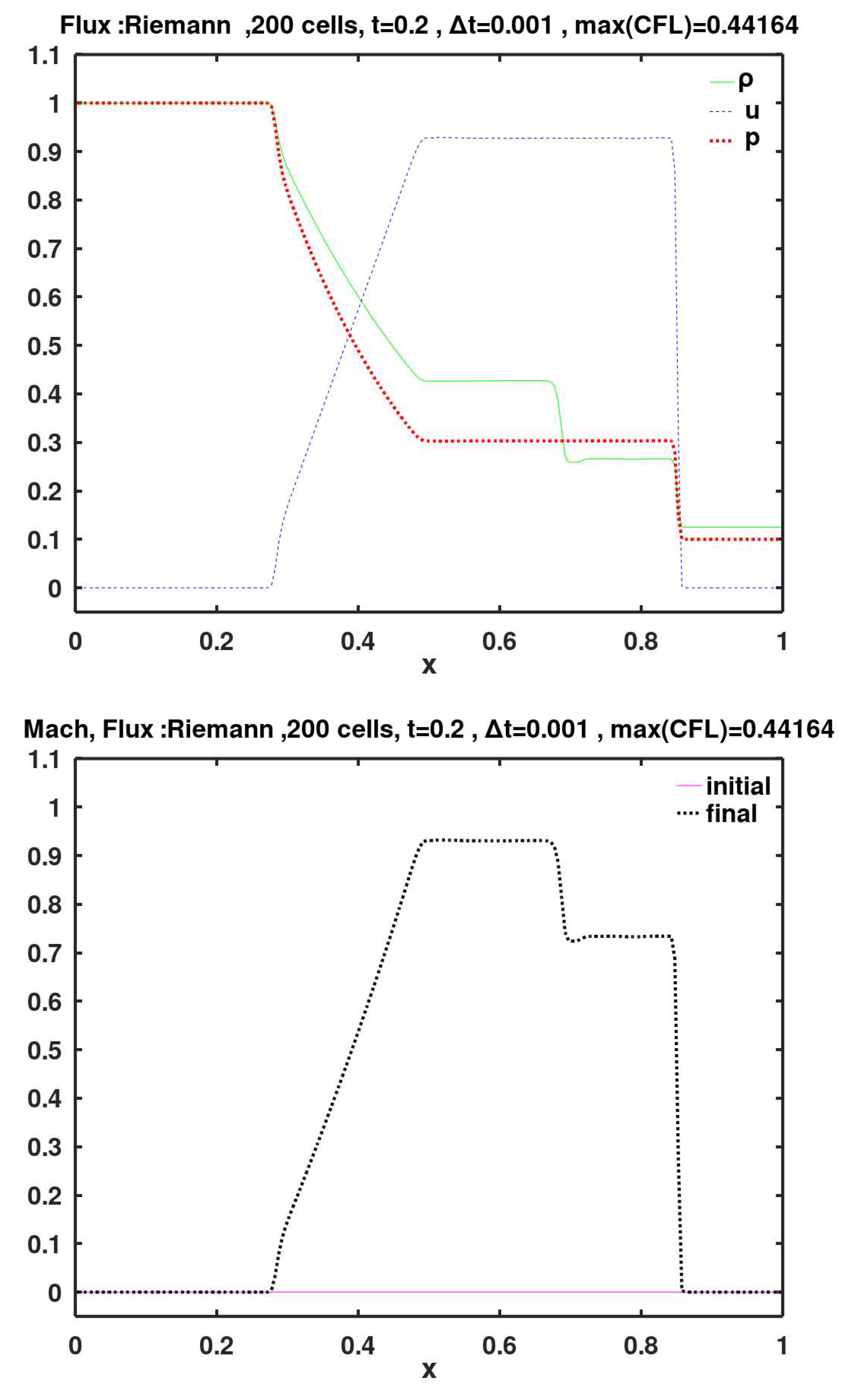
Figure 7.
Calculated final primitive variables and Mach number, using face flux of Roe.

Figure 8.
Calculated final primitive variables and Mach number, using face flux of Kurganov, Noelle, and Petrova (KNP).
Figure 8.
Calculated final primitive variables and Mach number, using face flux of Kurganov, Noelle, and Petrova (KNP).
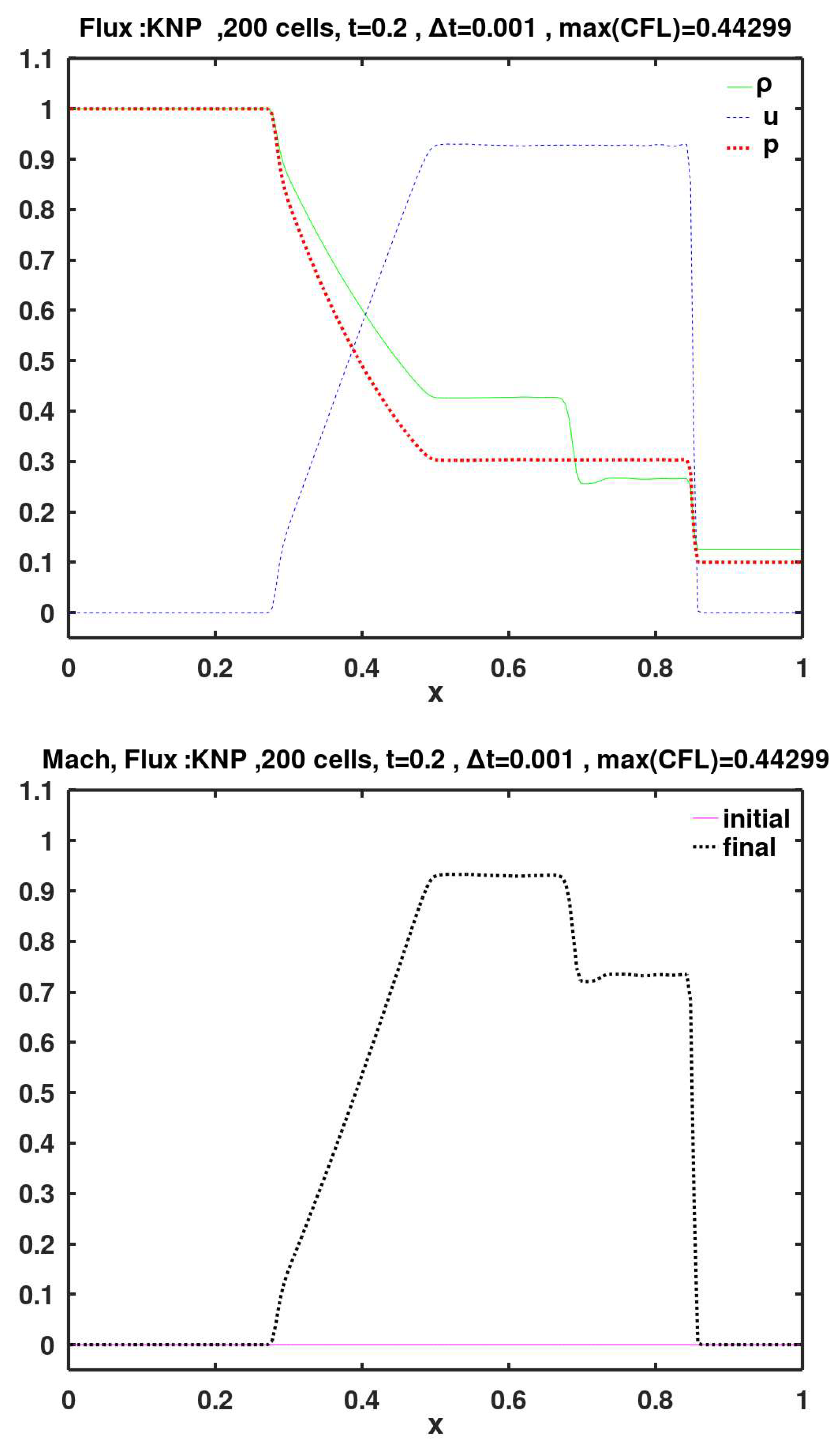
Figure 9.
Calculated final primitive variables and Mach number, using face flux of Kurganov and Tadmor (KT).
Figure 9.
Calculated final primitive variables and Mach number, using face flux of Kurganov and Tadmor (KT).
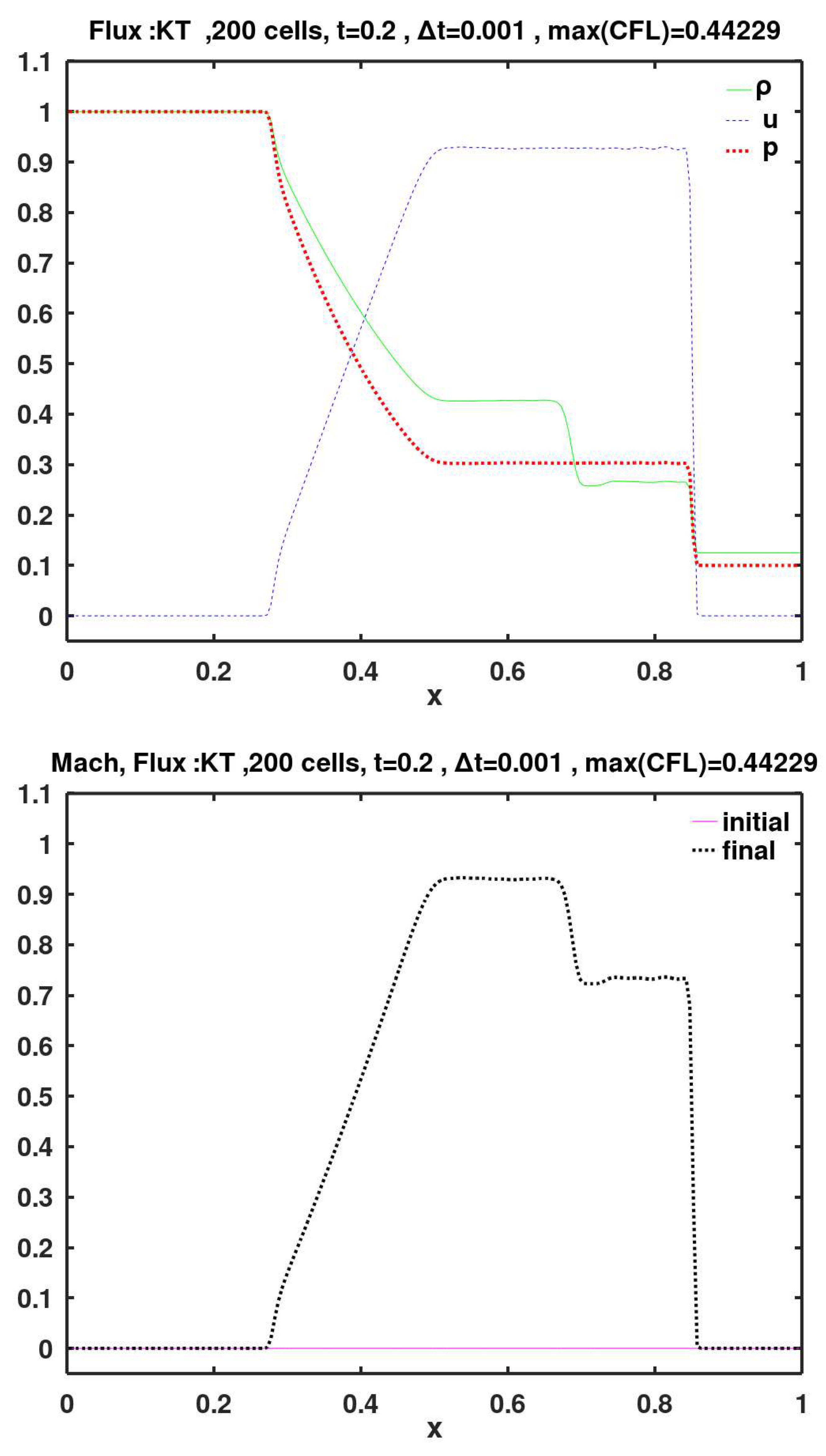
Figure 10.
Calculated final primitive variables and Mach number, using face flux of Steger and Warming (SW).
Figure 10.
Calculated final primitive variables and Mach number, using face flux of Steger and Warming (SW).
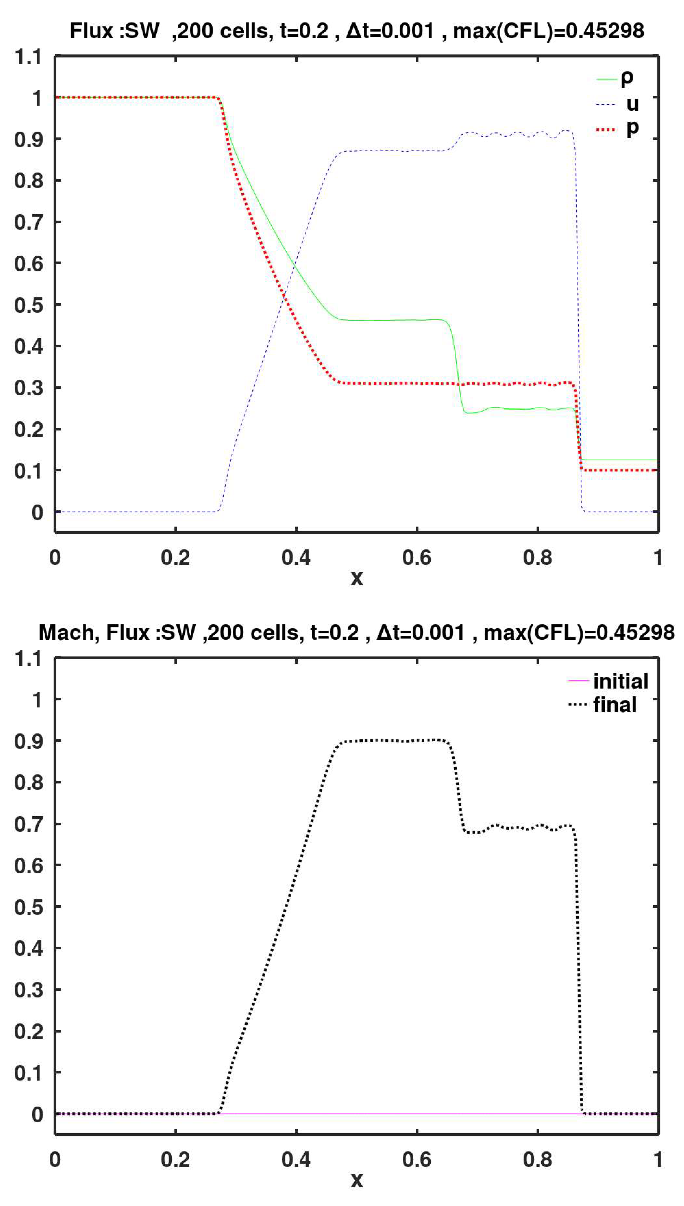
Figure 11.
Calculated final primitive variables and Mach number, using face flux of van Leer.
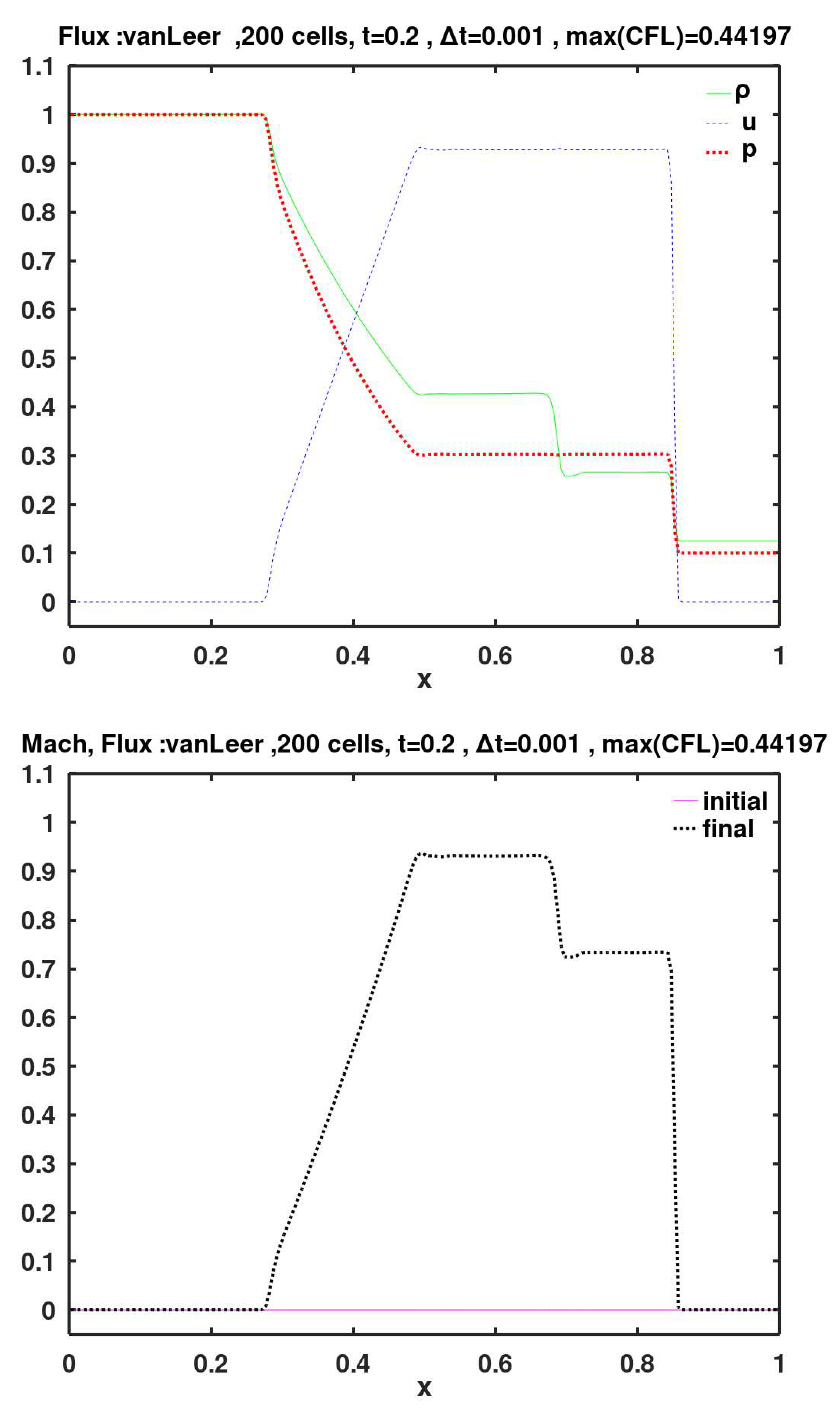
Figure 12.
Calculated final primitive variables and Mach number, using face flux of the Advection Upstream Splitting Method (AUSM).
Figure 12.
Calculated final primitive variables and Mach number, using face flux of the Advection Upstream Splitting Method (AUSM).
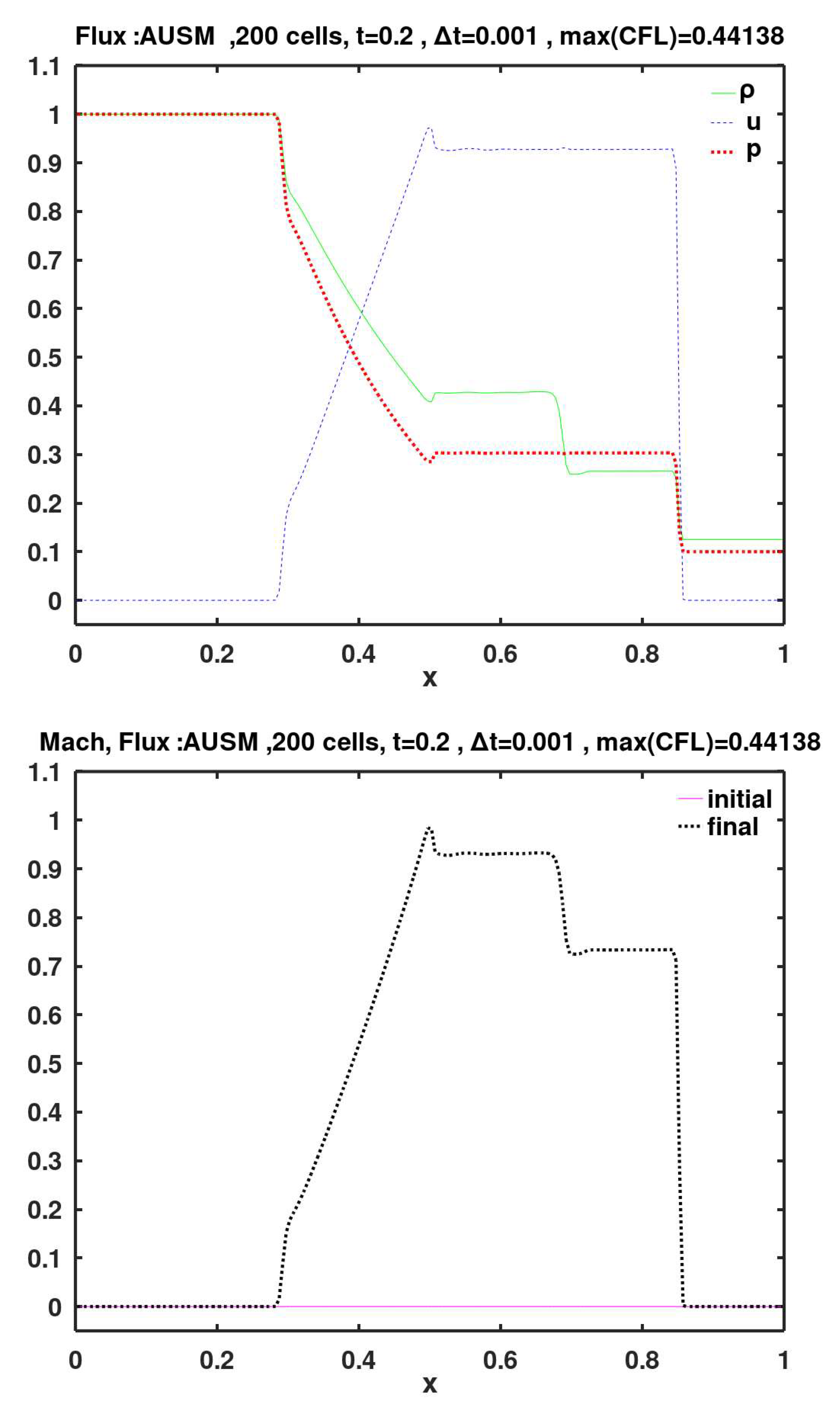
Figure 13.
Calculated final primitive variables and Mach number, using face flux of the first improved version of the Advection Upstream Splitting Method (AUSM+).
Figure 13.
Calculated final primitive variables and Mach number, using face flux of the first improved version of the Advection Upstream Splitting Method (AUSM+).
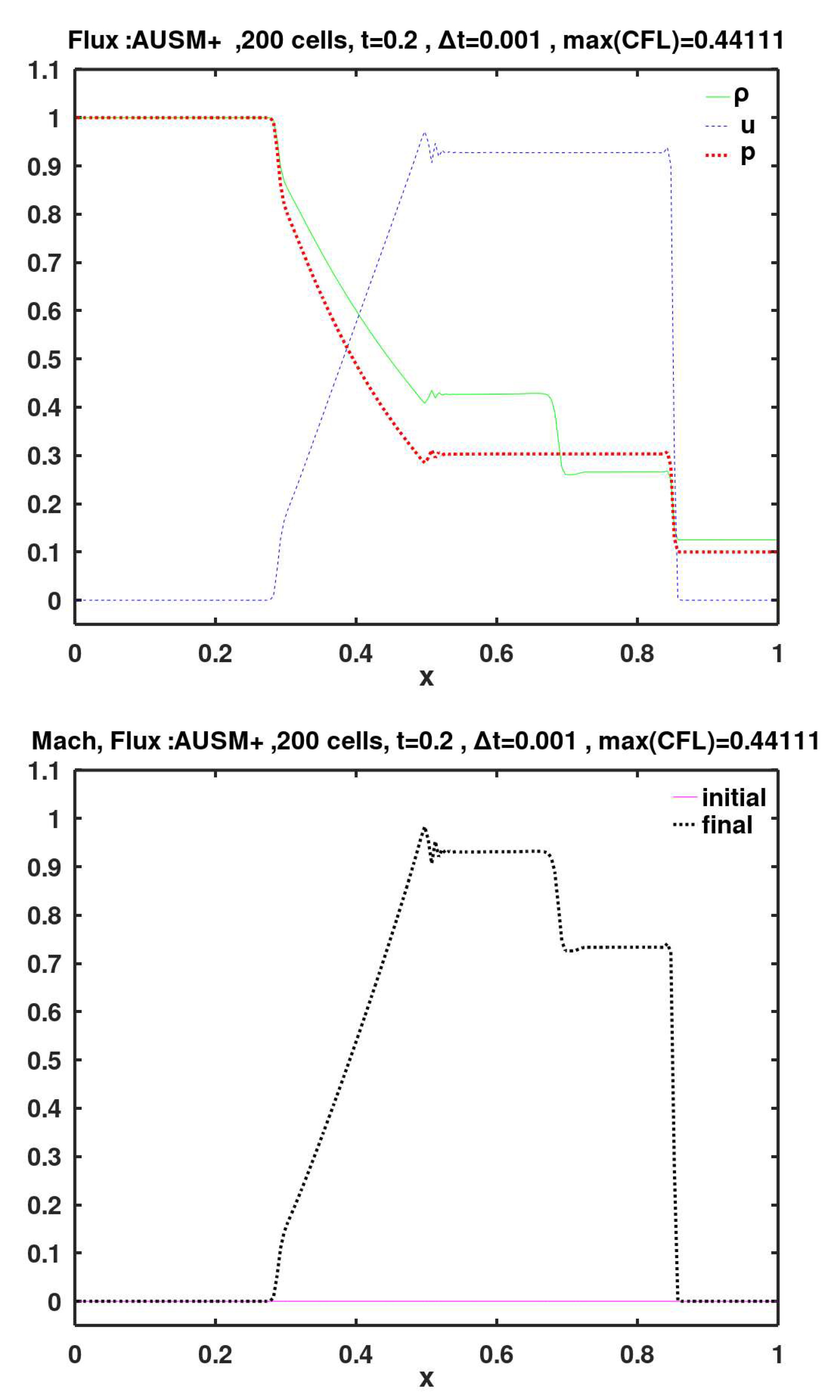
Figure 14.
Calculated final primitive variables and Mach number, using the face flux of the second improved version of the Advection Upstream Splitting Method (AUSM+-up, for all speeds).
Figure 14.
Calculated final primitive variables and Mach number, using the face flux of the second improved version of the Advection Upstream Splitting Method (AUSM+-up, for all speeds).
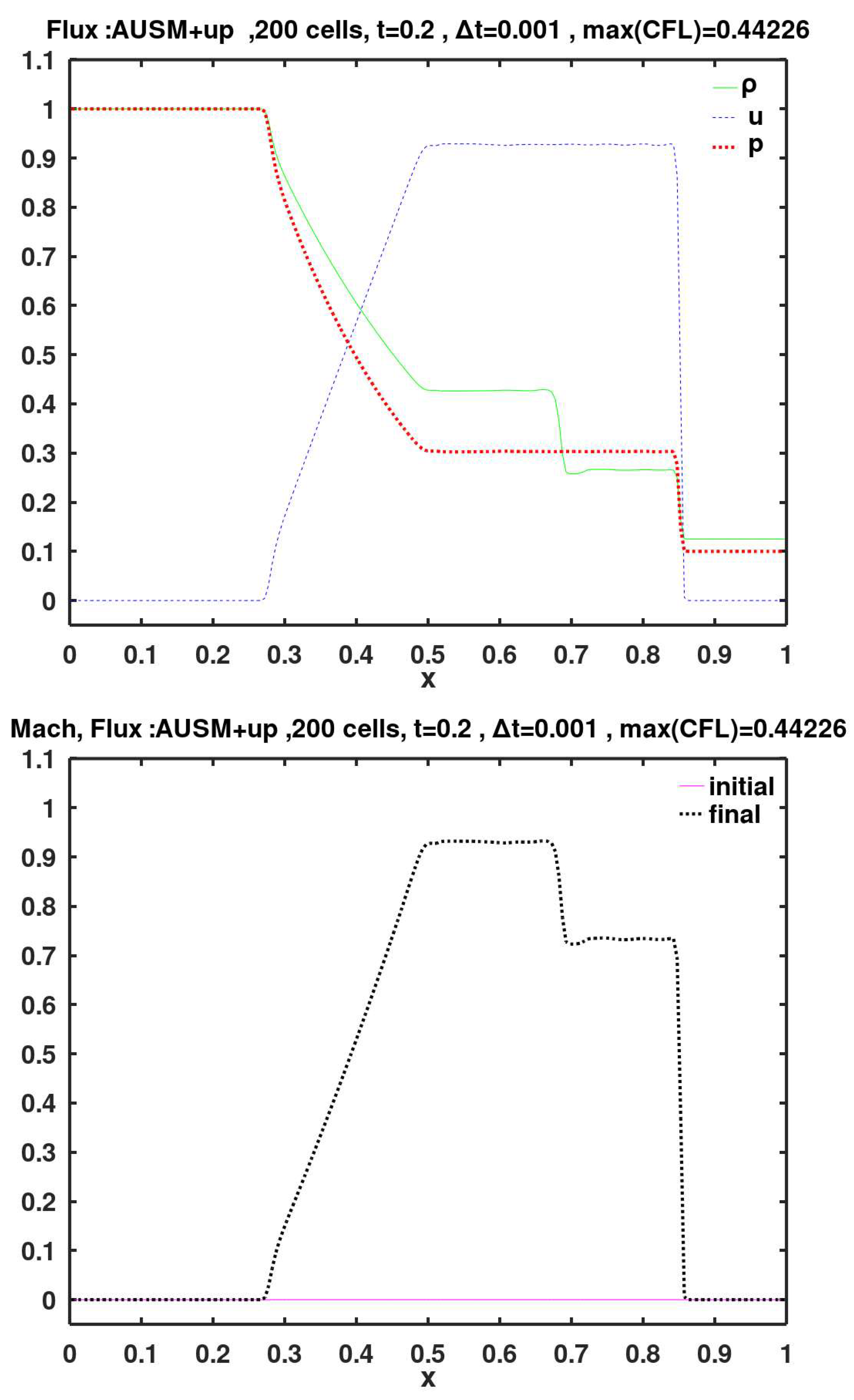
Figure 15.
Calculated final primitive variables and Mach number, using face flux of the Artificially Upstream Flux Vector Splitting (AUFS) method.
Figure 15.
Calculated final primitive variables and Mach number, using face flux of the Artificially Upstream Flux Vector Splitting (AUFS) method.

Figure 16.
Calculated final primitive variables and Mach number, using face flux of Harten, Lax, van Leer (HLL), along with the first estimation of Davis for the right/left wave speeds.
Figure 16.
Calculated final primitive variables and Mach number, using face flux of Harten, Lax, van Leer (HLL), along with the first estimation of Davis for the right/left wave speeds.
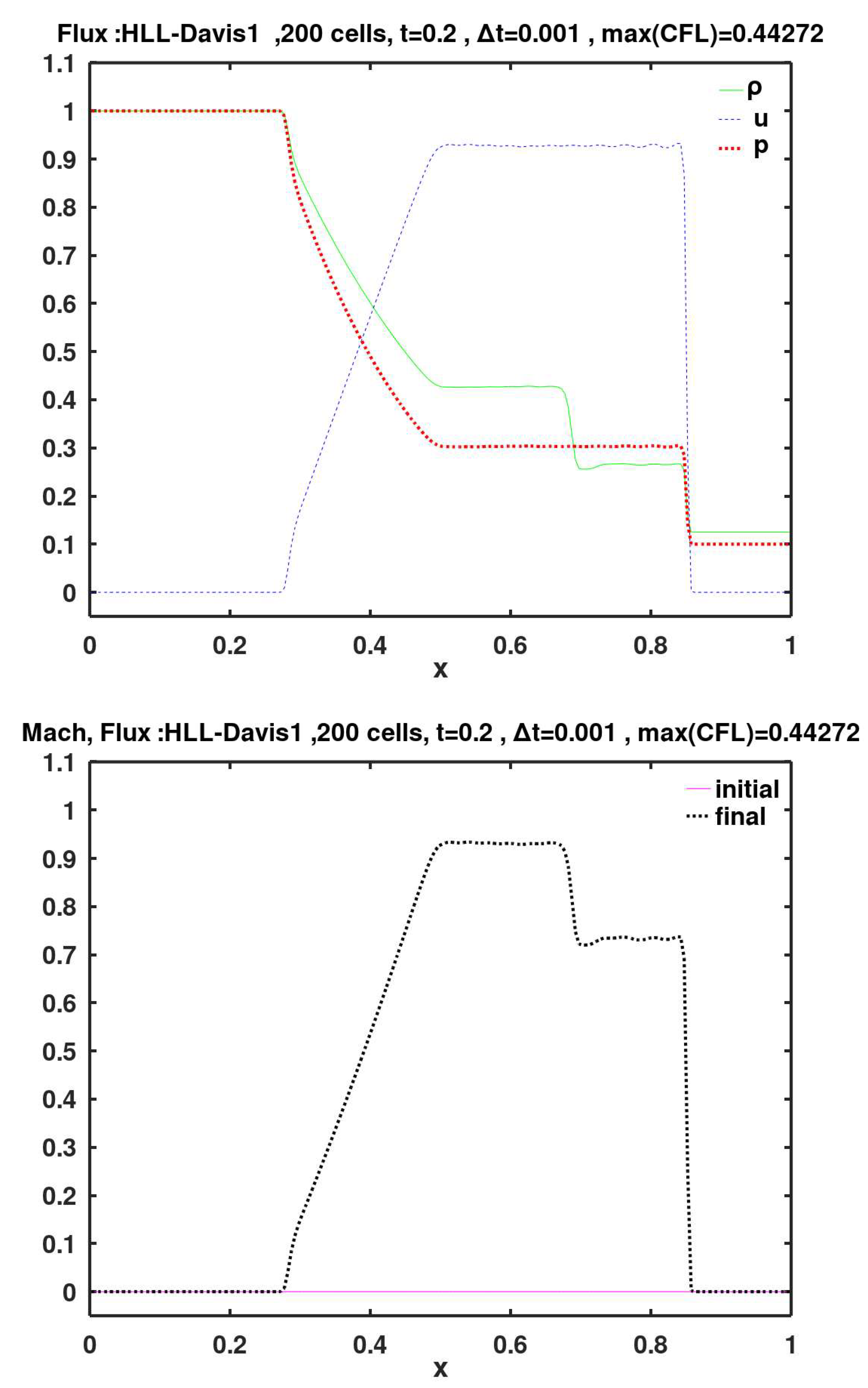
Figure 17.
Calculated final primitive variables and Mach number, using face flux of Harten, Lax, van Leer (HLL), along with the second estimation of Davis for the right/left wave speeds.
Figure 17.
Calculated final primitive variables and Mach number, using face flux of Harten, Lax, van Leer (HLL), along with the second estimation of Davis for the right/left wave speeds.
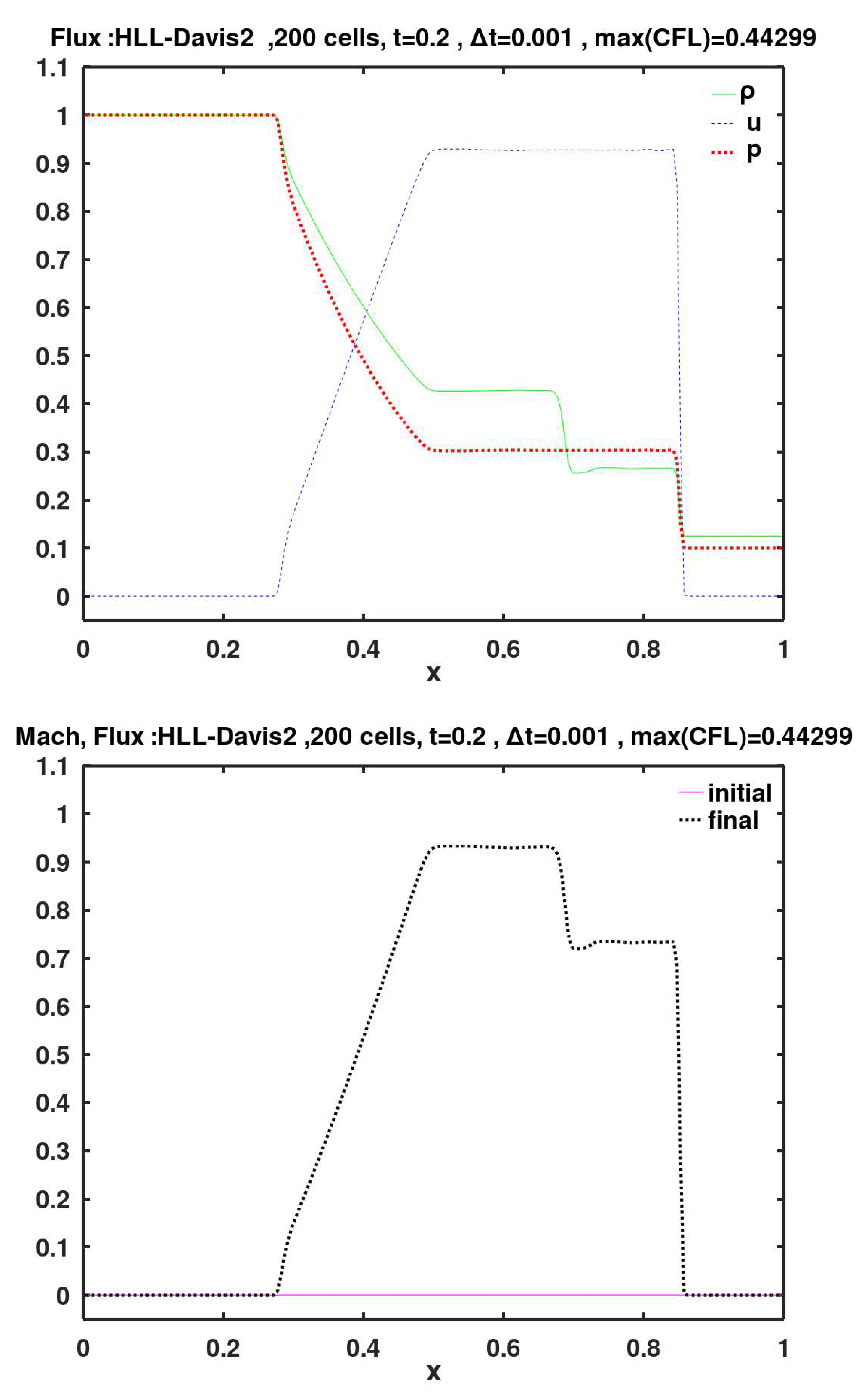
Figure 18.
Calculated final primitive variables and Mach number, using face flux of Harten, Lax, van Leer (HLL), along with the eigenvalues of Reo for the right/left wave speeds.
Figure 18.
Calculated final primitive variables and Mach number, using face flux of Harten, Lax, van Leer (HLL), along with the eigenvalues of Reo for the right/left wave speeds.
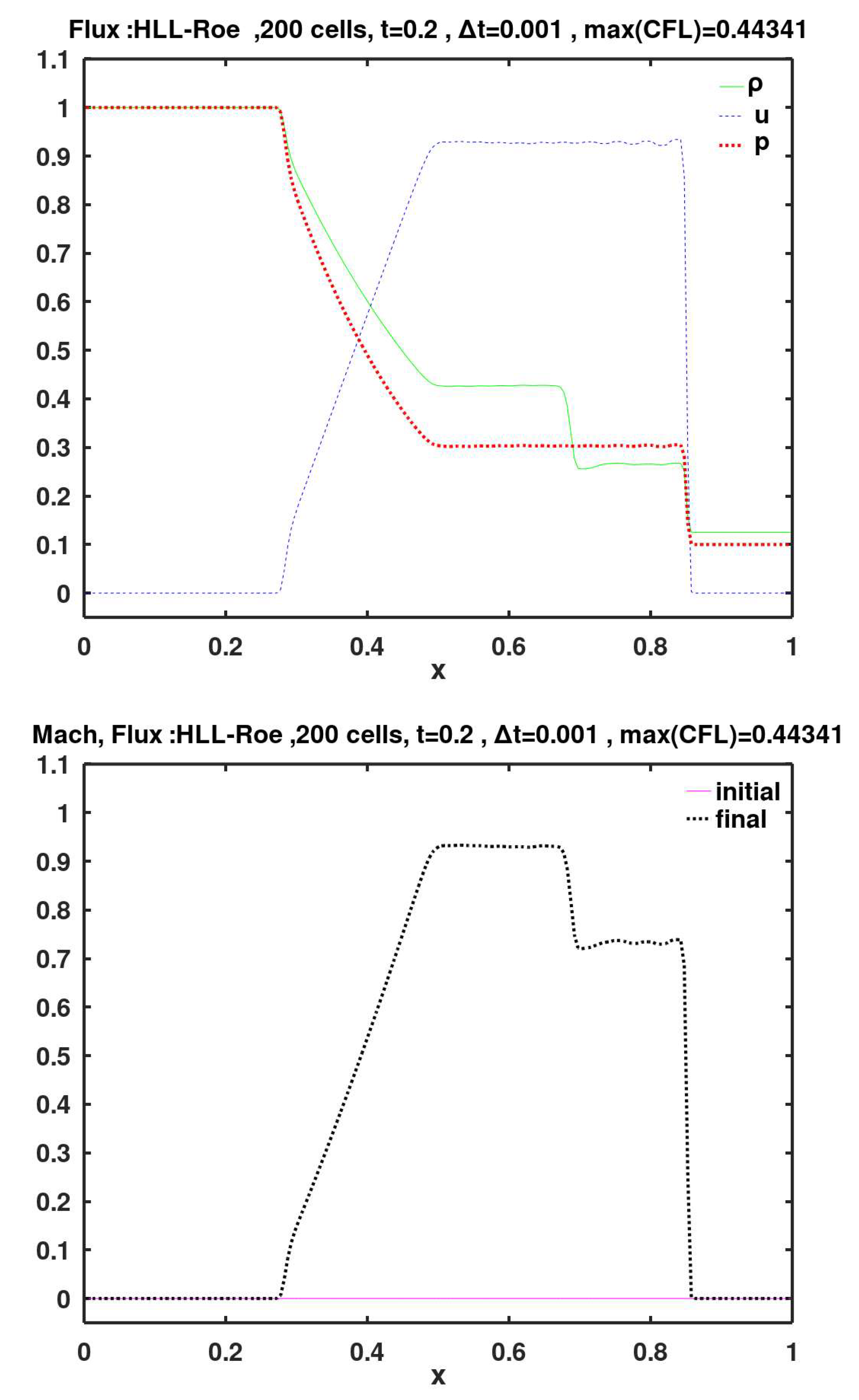
Figure 19.
Calculated final primitive variables and Mach number, using face flux of Harten, Lax, van Leer (HLL), along with the eigenvalues of Einfelt for the right/left wave speeds.
Figure 19.
Calculated final primitive variables and Mach number, using face flux of Harten, Lax, van Leer (HLL), along with the eigenvalues of Einfelt for the right/left wave speeds.
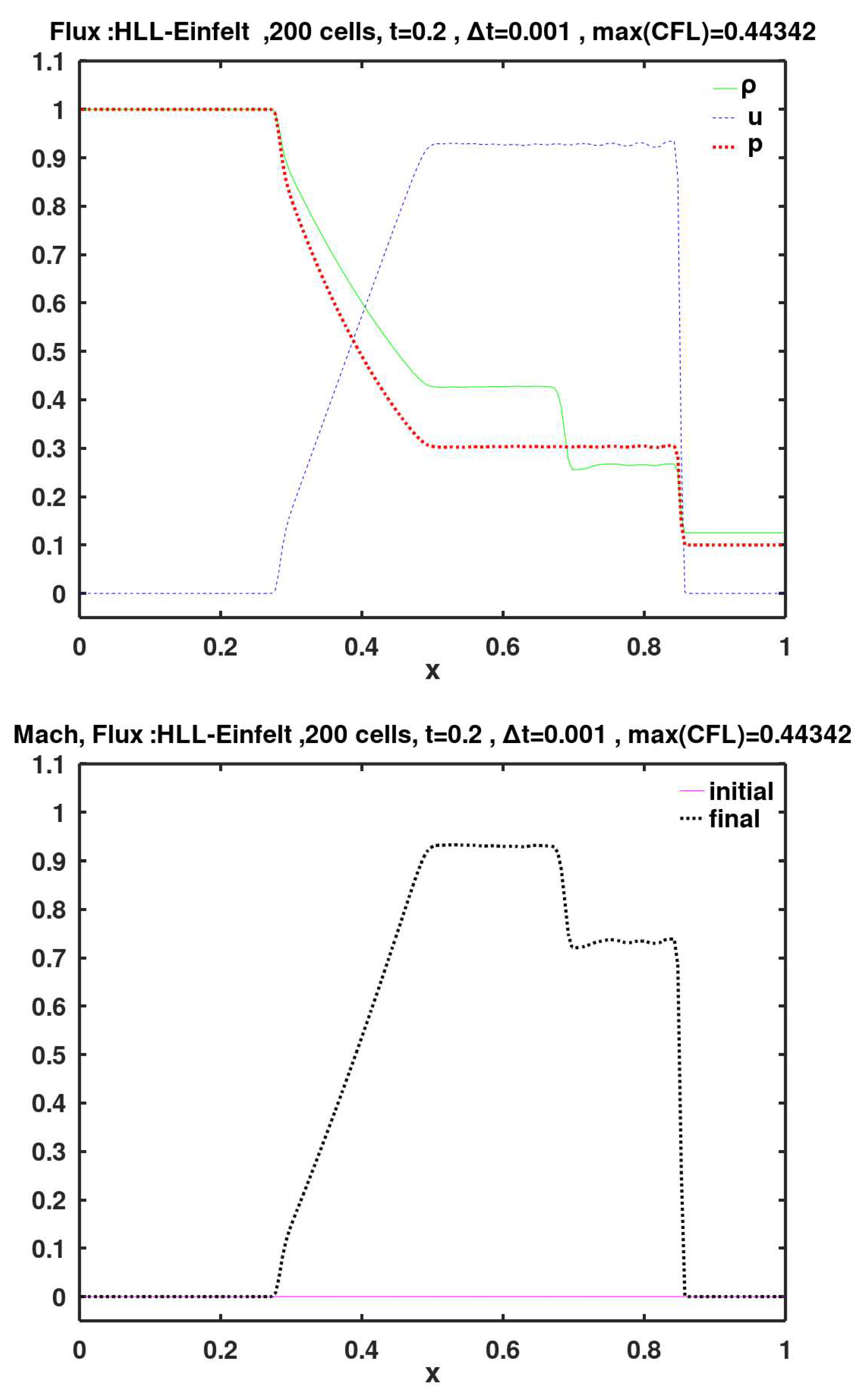
Figure 20.
Calculated final primitive variables and Mach number, using face flux of Harten, Lax, van Leer (HLL), along with pressure-based calculation for the right/left wave speeds.
Figure 20.
Calculated final primitive variables and Mach number, using face flux of Harten, Lax, van Leer (HLL), along with pressure-based calculation for the right/left wave speeds.
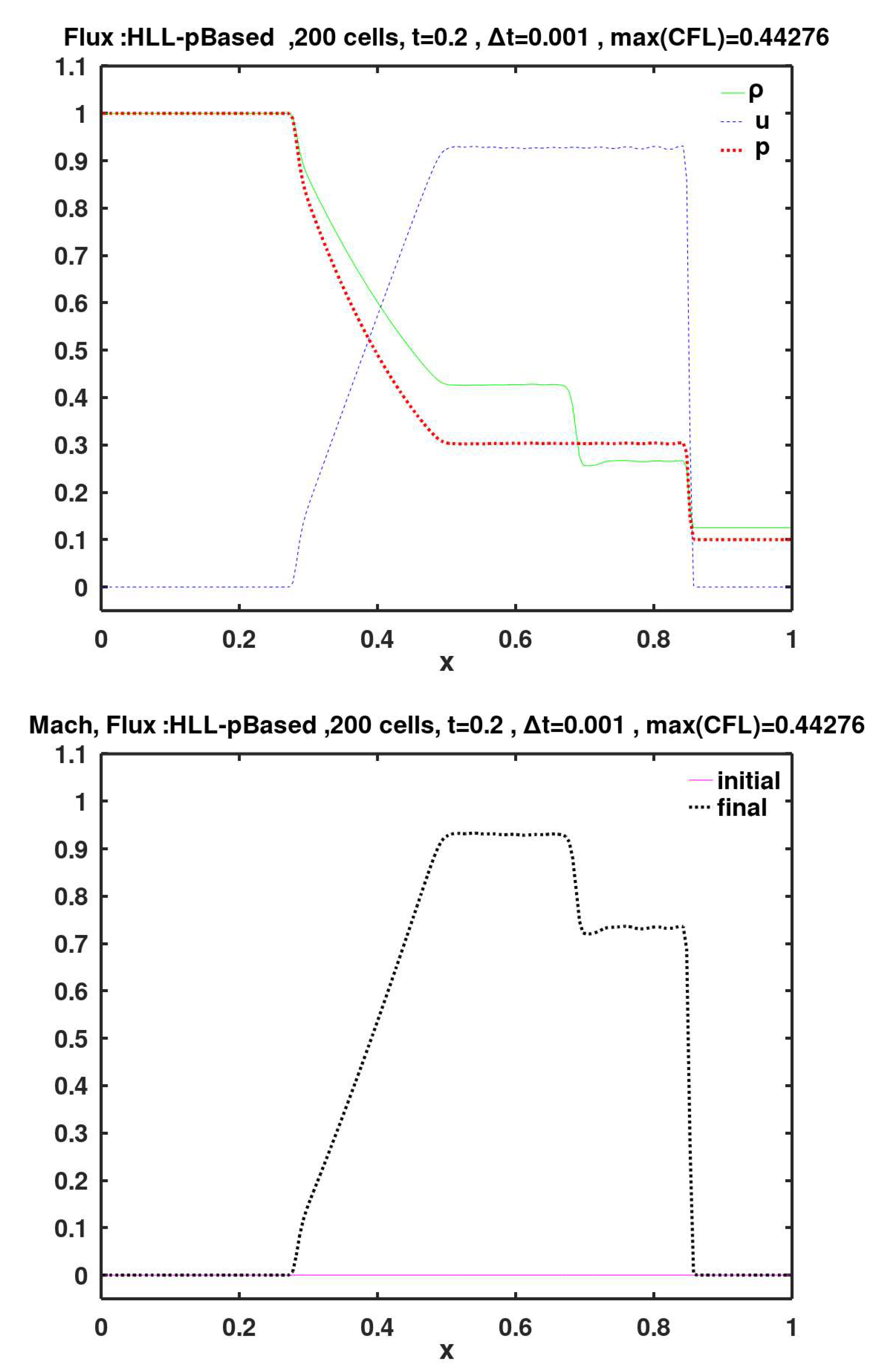
Figure 21.
Calculated final primitive variables and Mach number, using face flux of the improved version of Harten, Lax, van Leer (HLLC), along with the first estimation of Davis for the right/left wave speeds.
Figure 21.
Calculated final primitive variables and Mach number, using face flux of the improved version of Harten, Lax, van Leer (HLLC), along with the first estimation of Davis for the right/left wave speeds.
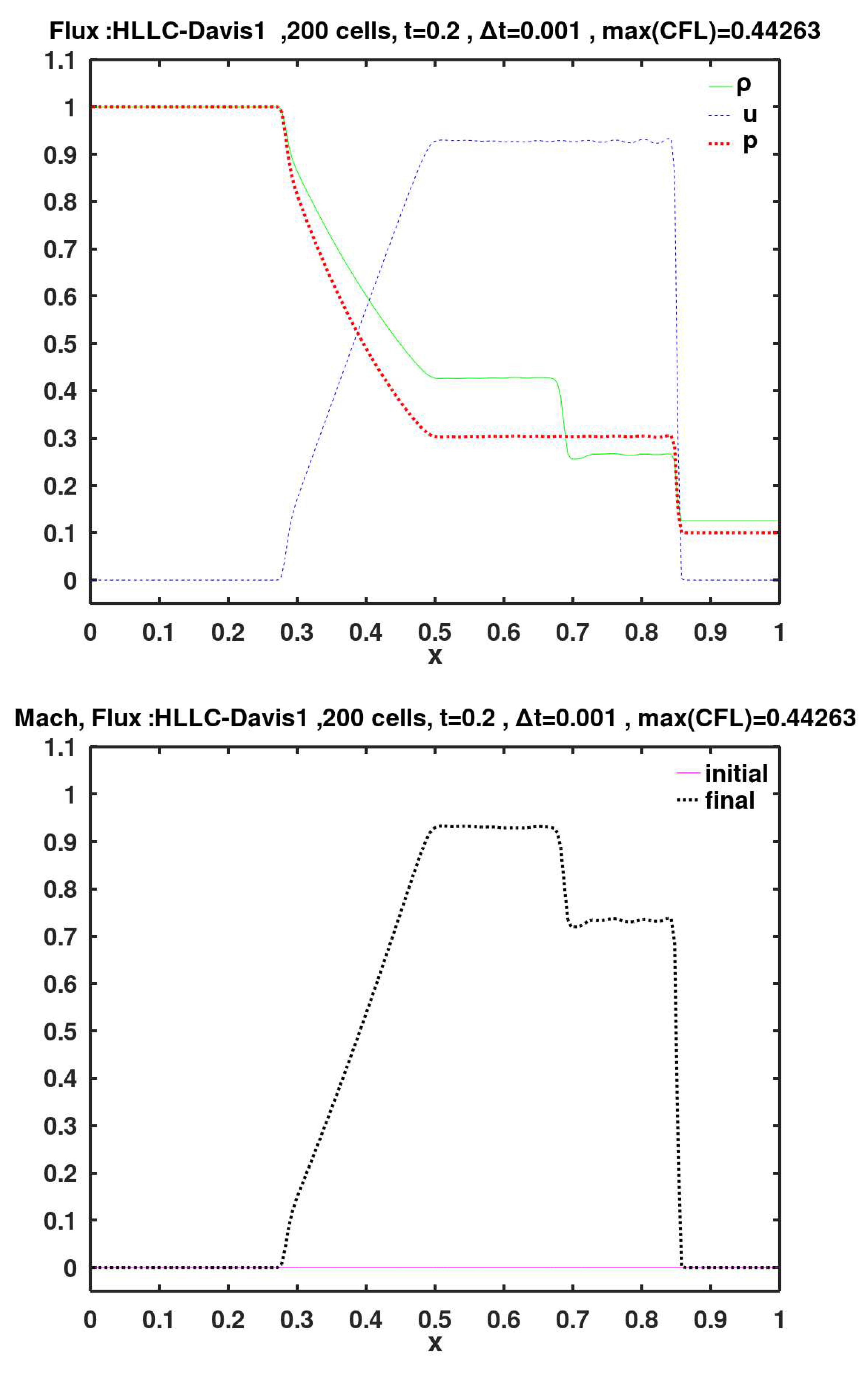
Figure 22.
Calculated final primitive variables and Mach number, using face flux of the improved version of Harten, Lax, van Leer (HLLC), along with the second estimation of Davis for the right/left wave speeds.
Figure 22.
Calculated final primitive variables and Mach number, using face flux of the improved version of Harten, Lax, van Leer (HLLC), along with the second estimation of Davis for the right/left wave speeds.
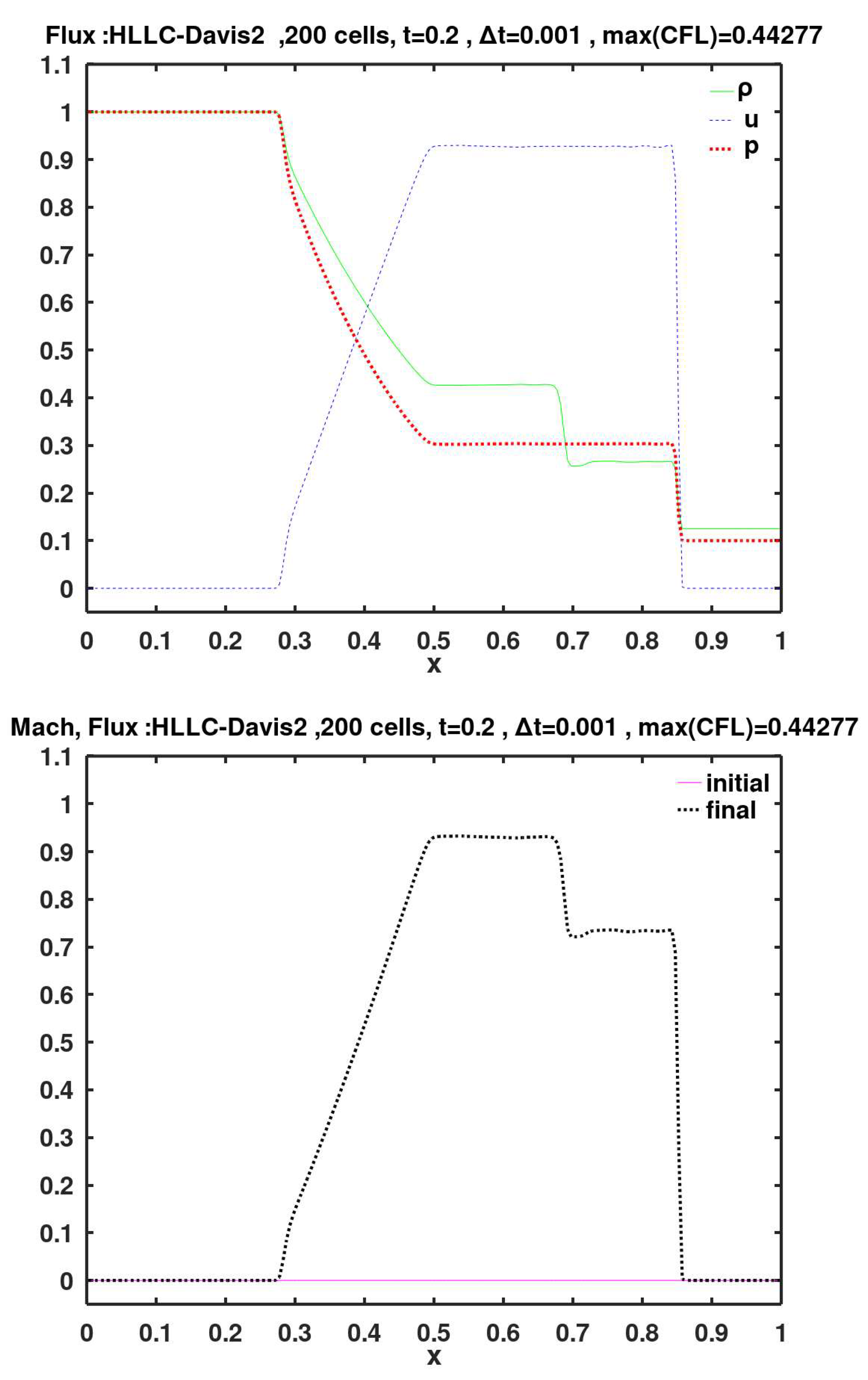
Figure 23.
Calculated final primitive variables and Mach number, using face flux of the improved version of Harten, Lax, van Leer (HLLC), along with the eigenvalues of Reo for the right/left wave speeds.
Figure 23.
Calculated final primitive variables and Mach number, using face flux of the improved version of Harten, Lax, van Leer (HLLC), along with the eigenvalues of Reo for the right/left wave speeds.
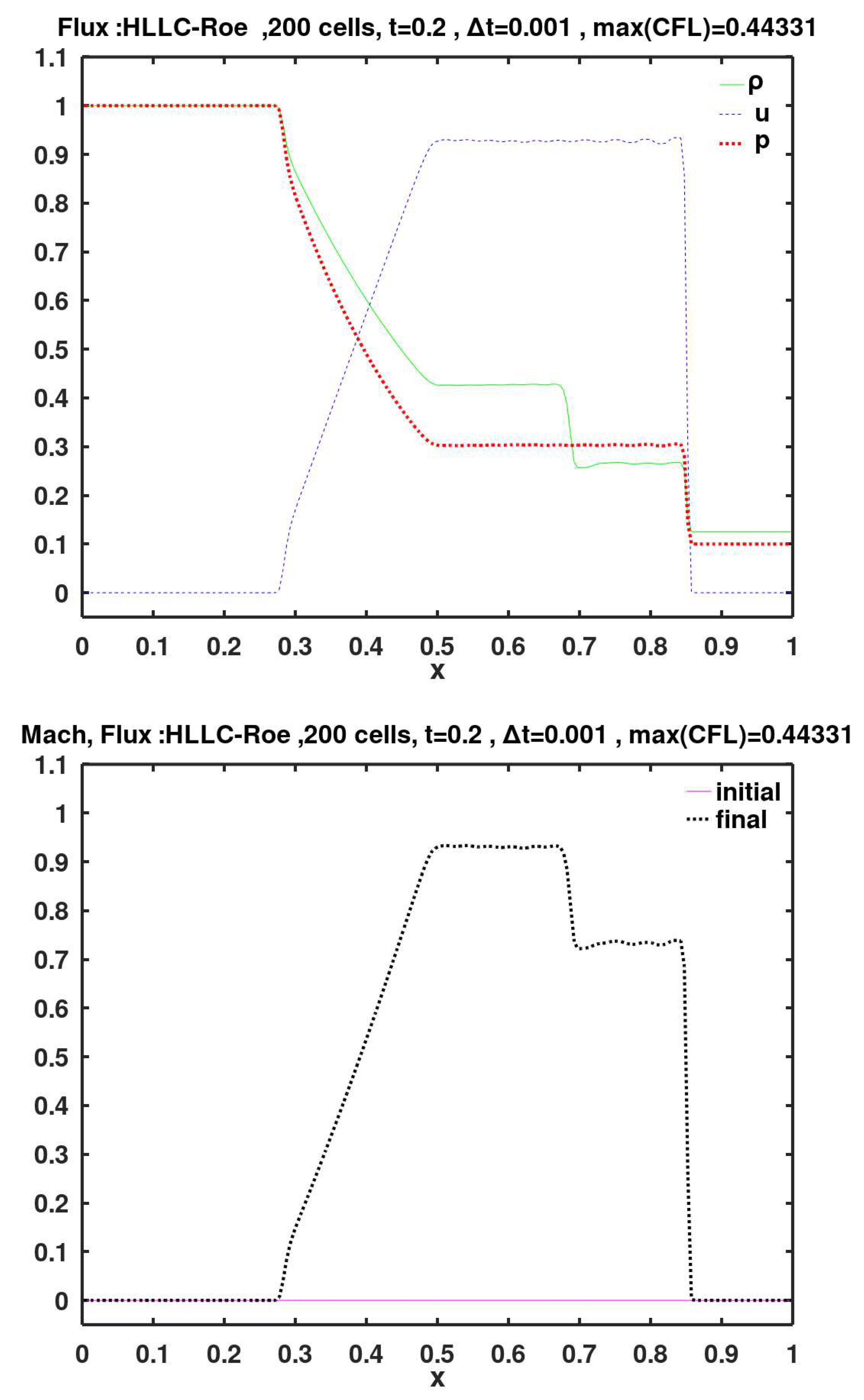
Figure 24.
Calculated final primitive variables and Mach number, using face flux of the improved version of Harten, Lax, van Leer (HLLC), along with the eigenvalues of Einfelt for the right/left wave speeds.
Figure 24.
Calculated final primitive variables and Mach number, using face flux of the improved version of Harten, Lax, van Leer (HLLC), along with the eigenvalues of Einfelt for the right/left wave speeds.
Figure 25.
Calculated final primitive variables and Mach number, using face flux of the improved version of Harten, Lax, van Leer (HLLC), along with pressure-based calculation for the right/left wave speeds.
Figure 25.
Calculated final primitive variables and Mach number, using face flux of the improved version of Harten, Lax, van Leer (HLLC), along with pressure-based calculation for the right/left wave speeds.
Figure 26.
Calculated final primitive variables and Mach number, using face flux of Lax and Friedrichs (LF).
Figure 26.
Calculated final primitive variables and Mach number, using face flux of Lax and Friedrichs (LF).
Figure 27.
Calculated final primitive variables and Mach number, using face flux of Rusanov.
8. Accuracy and Computational Efficiency
To quantity the closeness of each numerical solution to the exact one, the root-mean-square error (RMSE) for each primitive variable in addition to the Mach number were computed. Let denote any of these four quantities. At each cell-center, let the exact value be while the obtained one by numerically solving Euler equations using a certain flux method be . Then the RMSE for the generic variable is
where is an index for the cell-centers, and is the total number of cell-centers (which is 200 in this work).
The full list of these errors is given in Table 3. The flux methods are listed in the table in the same sequence of introducing them and presenting their graphical results earlier. The velocity seems to be the most challenging variable to predict, because it always has the highest RMSE value among the four quantities regardless of the flux method. Then comes the Mach number, which is based on the velocity.
The maximum magnitudes of the four quantities (density, gas velocity, pressure, and Mach number) in the exact solution are of the same order of magnitude. In addition, their individual RMSE values are also of the same order of magnitude. It may be then helpful to lump their RMSE values into a one measure of inaccuracy by simple addition, leading to a single aggregate RMSE for each flux method. This is done in Table 4. The methods are ordered ascendingly by that introduced aggregate RMSE. The method of AUFS comes first (aggregate RMSE = 0.05830). For all flux methods other than AUSM+-up, AUSM, SW and LF, the aggregate RMSE increases gradually with small increments from a method to the next better one up to AUSM+ (aggregate RMSE = 0.06651). This is followed by a mild increase with the two methods AUSM+-up (aggregate RMSE = 0.07285) and AUSM (aggregate RMSE = 0.07499). Then, as the end of the list, the aggregate RMSE jumps by a factor of about 4 for the SW and LF methods, thereby clearly delineating their solutions as improper.
While the accuracy of a flux method is very important when analyzing it, its computational demand is worthy of consideration. In large three-dimensional finite volume simulations, face flux construction is a process that happens millions of times to advance the solution by just one time step, and the solution may need thousands of time steps to complete. Even an extremely small time saving in the calculation of the flux vector at a face can thus have a useful impact when considering the total runtime of a realistic simulation. The elapsed clock time of the simulation excluding the processes of initializing variables, calculating an exact solution (as a reference to compare with), plotting results, or writing output data files was recorded for each flux method, and the results are presented in Table 5 in an ascending order. It is worthy of mentioning here that the relative time (one method relative to another) is more meaningful than the absolute time spent. The computing machine used in this work is a laptop Dell Inspiron (model N5010), with 6 GB of installed RAM memory and an Intel® CoreTM i5 CPU, M 480 @ 2.67GHz. The SW method took the shortest time of 41.13235 s, while the Riemann exact solver took the longest time of 46.49466 s. The ratio of these two extrema values is 1.13037.
A percentage increase of the runtime (using the shortest recorded one as a reference) is included in Table 5. This relative measure of computational cost is calculated as
The changes in the elapsed time are not large, with an extra time penalty not exceeding 13% when using the exact Riemann solver flux method (as the one found to be the most computationally demanding) compared to any other method. This can be attributed to the inherent simplicity of the problem.
9. Conclusions
Face flux construction is a core task in a finite volume solver. An end user of such a solver may be offered a large number of flux methods to select from for numerically handling convection (divergence) terms (OpenCFD, 2020). A good background in flux construction methods as well as an elementary analysis of their performance for a simple problem having a known analytical solution may help in making a good selection of a flux method in relevant simulations.
In this context, this work considered 22 flux methods and analyzed them while solving the Sod problem (a classical one-dimensional jump problem for an inviscid flow). Other than changing the flux method as the only discrete variable to examine its influence, the analysis is conducted at a set of unified conditions, where a fully-extrapolated version of the MUSCL scheme was used in which the classical van Leer flux limiter was employed. The one-dimensional grid was uniformly-spaced 200 cells, and the maximum CFL number was kept around 0.44. Qualitative and quantitative assessment of the accuracy of the resulting solution as well its estimated computational cost suggest that there is a number of methods that can offer similar levels of a good performance, including the methods of Kurganov-Noelle-Petrova, van Leer, Harten-Lax-van Leer-Davis2, and Harten-Lax-van Leer-Contact-Davis2. On the other hand, two flux methods may be avoided due to high oscillation or excessive dissipation.
Acknowledgment
Dr. Michael Zingale, Associate Professor at Stony Brook University in the Department of Physics and Astronomy (Stony Brook, New York, U.S.A.), is highly appreciated for the kind permission of using a figure of the Castro project for validation purpose here.
References
- Riemann, B. , 1860. Über die Fortpflanzung ebener Luftwellen von endlicher Schwingungsweite [On the propagation of plane air waves of finite amplitude], Abhandlungen der Königlichen Gesellschaft der Wissenschaften zu Göttingen, vol. 8, pp. 43–65 (in German).
- Castro-Orgaz, O.; and Hager W., H. , 2019. The Riemann Problem. In: Shallow Water Hydraulics, pp. 313-346, Springer, Cham. [CrossRef]
- Kamm, James Russell, 2015. An Exact, Compressible One-Dimensional Riemann Solver for General, Convex Equations of State, Report LA-UR-15-21616, Los Alamos National Laboratory, USA.
- Hantke, Maren; Matern, Christoph; Ssemaganda, Vincent; and Warnecke, Gerald, 2020. The Riemann problem for a weakly hyperbolic two-phase flow model of a dispersed phase in a carrier fluid, Quarterly of Applied Mathematics, vol. 78, pp. 431-467. [CrossRef]
- Fletcher, C. A. J. , 1991. Computational Techniques for Fluid Dynamics, Volume II, Second Edition, Springer-Verlag, Germany. [CrossRef]
- Hoffmann, K. A. and Chiang, S. T., 1993. Computational Fluid Dynamics for Engineers - Volume II, Engineering Education System, Wichita, Kansas, USA.
- Fletcher, D. G. 2004. FUNDAMENTALS OF HYPERSONIC FLOW-AEROTHERMODYNAMICS, Paper presented at the RTO AVT Lecture Series on "Critical Technologies for Hypersonic Vehicle Development", held at the von Kármán Institute, Rhode-St-Genèse, Belgium, 10-14 May, 2004, and published in RTO-EN-AVT-116.
- Ames Research Staff, NACA, 1953. Equations, Tables, and Charts for Compressible Flow, NACA Report 1135, Ames Aeronautical Laboratory, California, USA.
- Laney, Culbert B., 1998. Computational Gasdynamics, Cambridge University Press, USA, ISBN 9780511605604. [CrossRef]
- Sod, Gary A., 1978. A survey of several finite difference methods for systems of nonlinear hyperbolic conservation laws, Journal of Computational Physics, vol. 27(1), pp. 1-31. [CrossRef]
- Kuznetsov, Nikolai M., 2000. Stability of Shock Waves. In: Handbook of Shock Waves, Three Volume Set (Gabi Ben-Dor, Ozer Igra, Tov Elperin, Editors), Elsevier, pp. 413-454.
- Eaton, John W., 2020. About GNU Octave, online resource, accessed 9/June/2020. Available online: https://www.gnu.org/software/octave/about.html.
- Rankine, William John Macquorn, 1870. On the thermodynamic theory of waves of finite longitudinal disturbances, Philosophical Transactions of the Royal Society of London, vol. 160, pp. 277–288. [CrossRef]
- Hugoniot, H. , 1887. Mémoire sur la propagation des mouvements dans les corps et spécialement dans les gaz parfaits (première partie) [Memoir on the propagation of movements in bodies, especially perfect gases (first part)], Journal de l'École Polytechnique, vol 57, pp. 3–97.
- Hugoniot, H. , 1889. Mémoire sur la propagation des mouvements dans les corps et spécialement dans les gaz parfaits (deuxième partie) [Memoir on the propagation of movements in bodies, especially perfect gases (second part)], Journal de l'École Polytechnique, vol. 58, pp. 1–125.
- Szabo, A.; and Szabo, A. , Modified “Rankine-Hugoniot” shock fitting technique: Simultaneous solution for shock normal and speed, Journal of Geophysical Research, vol. 112, paper A101100 (9 pages). [CrossRef]
- Castro, a massively parallel code that solves the multicomponent compressible hydrodynamic equations for astrophysical flows, Verification, Hydrodynamics Test Problems, Sod’s Problem (and Other Shock Tube Problems), online resource, accessed 25/May/2020. Available online: https://amrex-astro.github.io/Castro/docs/Verification.html#sods-problem-and-other-shock-tube-problems.
- Godunov, Sergei K., 1959. A difference scheme for numerical computation of discontinuous solution of hyperbolic equation, (Russian, translated), Matematicheskii Sbornik, vol. 47, pp. 271–306.
- van Leer, Bram, 1979. Towards the ultimate conservative difference scheme. V. A second-order sequel to Godunov's method, Journal of Computational Physics, vol. 32(1), pp. 101-136. [CrossRef]
- Waterson, N. P. , Deconinck, H. 2007. Design principles for bounded higher-order convection schemes – a unified approach, Journal of Computational Physics, vol. 224, pp. 182–207. [CrossRef]
- van Leer, Bram, 1974. Towards the ultimate conservative difference scheme. II. Monotonicity and conservation combined in a second-order scheme, Journal of Computational Physics, vol. 14(4), pp. 361-370. [CrossRef]
- Chu, Vincent H.; and Gao, Congwei, 2013. FALSE DIFFUSION PRODUCED BY FLUX LIMITERS, Computational Thermal Sciences: An International Journal, vol. 5(6), pp. 503-520. [CrossRef]
- Li, Guangning; Bhatia, Dinesh; and Wang, Jian, 2020. Compressive properties of Min-mod-type limiters in modelling shockwave-containing flows, Journal of the Brazilian Society of Mechanical Sciences and Engineering , vol. 42, article number 290 (20 pages). Available online: https://link.springer.com/article/10.1007%2Fs40430-020-02374-7.
- Bai, Feng-peng; Yang, Zhong-hua; and Zhou, Wu-gang, 2018. Study of total variation diminishing (TVD) slope limiters in dam-break flow simulation, Water Science and Engineering, vol. 11(1), pp. 68-74. [CrossRef]
- Strikwerda, John C., 2004. Finite Difference Schemes and Partial Differential Equations, Second Edition, SIAM (society of industrial and applied mathematics), ISBN 978-0-89871-567-5. [CrossRef]
- Roe, P. L. ; 1981. Approximate Riemann solvers, parameter vectors, and difference schemes, Journal of Computational Physics, vol. 43(2), pp. 357-372. [CrossRef]
- Kurganov, Alexander; Noelle, Sebastian; and Petrova, Guergana, 2001. Semidiscrete Central-Upwind Schemes for Hyperbolic Conservation Laws and Hamilton--Jacobi Equations, SIAM Journal on Scientific Computing, vol. 23(3), pp. 707-740. [CrossRef]
- Kurganov, Alexander; and Tadmor, Eitan, 2000. New high-resolution central schemes for nonlinear conservation laws and convection–diffusion equations, Journal of Computational Physics, vol. 160(1), pp. 241–282. [CrossRef]
- Steger, Joseph L.; and Warming, R. F., 1979. Flux vector splitting of the inviscid gasdynamic equations with application to finite-difference methods, NASA Technical Memorandum NASA-TN-78605, 53 pages.
- Steger, Joseph L.; and c, R. F., 1981. Flux vector splitting of the inviscid gasdynamic equations with application to finite-difference methods, Journal of Computational Physics, vol. 40(2), pp. 263-293. [CrossRef]
- van Leer, B. , 1982. Flux-vector splitting for the Euler equations. In: E. Krause (Editor) Eighth International Conference on Numerical Methods in Fluid Dynamics, Lecture Notes in Physics, vol. 170, Springer, Berlin, Heidelberg, ISBN 978-3-540-11948-7. [CrossRef]
- Liou, Meng-Sing and Steffen, Christopher J. Jr.; 1993. A New Flux Splitting Scheme, Journal of Computational Physics, vol. 107(1), pp. 23-39. [CrossRef]
- Liou, Meng-Sing, 1996. A Sequel to AUSM: AUSM+, Journal of Computational Physics, vol. 129(2), pp. 364-382. [CrossRef]
- Liou, Meng-Sing, 2006. A sequel to AUSM, Part II: AUSM+-up for all speeds, Journal of Computational Physics, vol. 214(1), pp. 137-170. [CrossRef]
- Sun, M.; and Takayama, K. , 2003. An artificially upstream flux vector splitting scheme for the Euler equations, Journal of Computational Physics, vol. 189(1), pp. 305-329. [CrossRef]
- Harten, Amiram; Lax, Peter D.; and van Leer, Bram, 1983. On Upstream Differencing and Godunov-Type Schemes for Hyperbolic Conservation Laws, SIAM Review, vol. 25(1), pp. 35–61. [CrossRef]
- Davis, S. F. , 1988. Simplified Second-Order Godunov-Type Methods, SIAM Journal on Scientific and Statistical Computing, vol. 9(3), pp. 445–473. [CrossRef]
- Einfeldt, Bernd, 1988. On Godunov-Type Methods for Gas Dynamics, SIAM Journal on Numerical Analysis, vol. 25(2), pp. 294–318. [CrossRef]
- Toro, E. F.; Spruce, M.; and Speares, W. , 1994. Restoration of the contact surface in the HLL-Riemann solver, Shock Waves, vol. 4, pp. 25–34. [CrossRef]
- Toro, E. F.; Spruce, M.; and Speares, W. 1992. Restoration of the contact surface in the HLL Riemann solver, Report CoA 9204, Cranfield Institute of Technology, UK.
- Lax, Peter D., 1954. Weak solutions of nonlinear hyperbolic equations and their numerical computation, Communications on Pure and Applied Mathematics, vol. 7, pp. 159–193. [CrossRef]
- Rusanov, V. V. , 1970. On difference schemes of third order accuracy for nonlinear hyperbolic systems, Journal of Computational Physics, vol. 5(3), pp. 507-516. [CrossRef]
- Chang, S. C.; and Wang, X. Y. 2003. Multi-Dimensional Courant Number Insensitive CE/SE Euler Solvers for Applications Involving Highly Nonuniform Meshes, AIAA Paper 2003-5285, presented at the 39th AIAA/ASME/SAE/ASEE Joint Propulsion Conference and Exhibit, July 20-23, 2003, Huntsville, Alabama, USA.
- OpenCFD Ltd., (an affiliate of ESI Group), OpenFOAM User Guide v1912, Divergence schemes, online resource, accessed 10/Jun/2020. Available online: https://www.openfoam.com/documentation/guides/latest/doc/guide-schemes-divergence.html.
Figure 1.
Illustration of the Riemann problem. For a shock tube, the initial velocities are zeros.
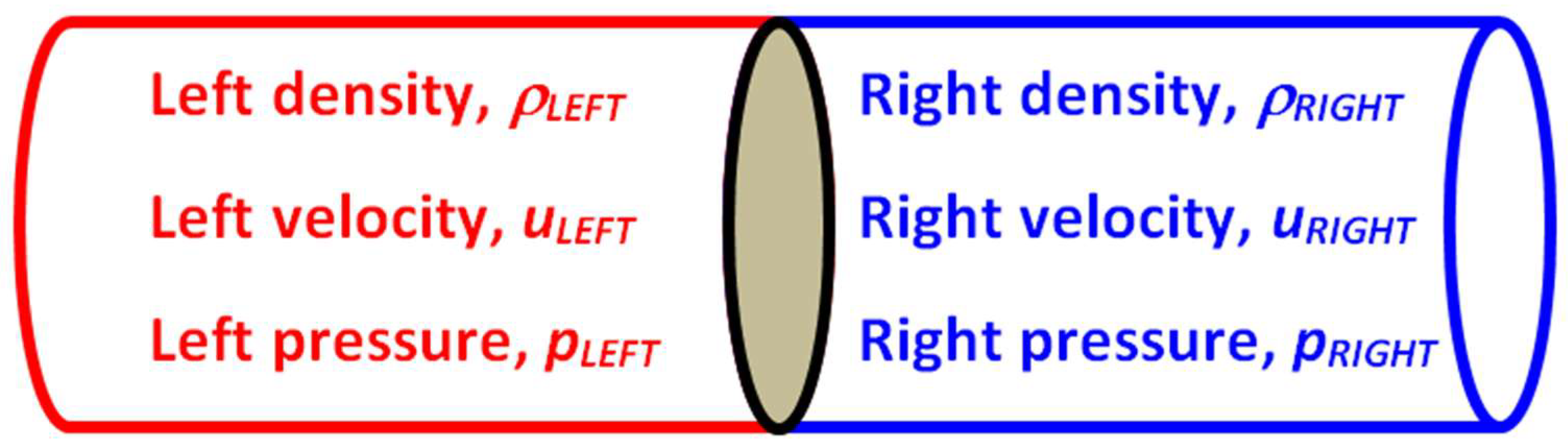
Figure 2.
Initial primitive variables in the Sod problem.
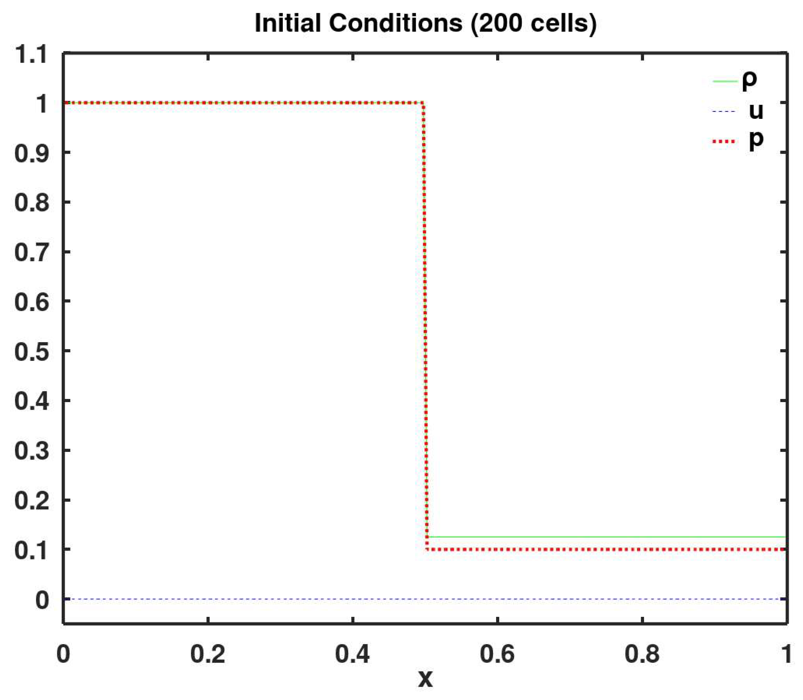
Figure 3.
Exact (analytical) final primitive variables and the initial and exact (analytical) final Mach number.
Figure 3.
Exact (analytical) final primitive variables and the initial and exact (analytical) final Mach number.
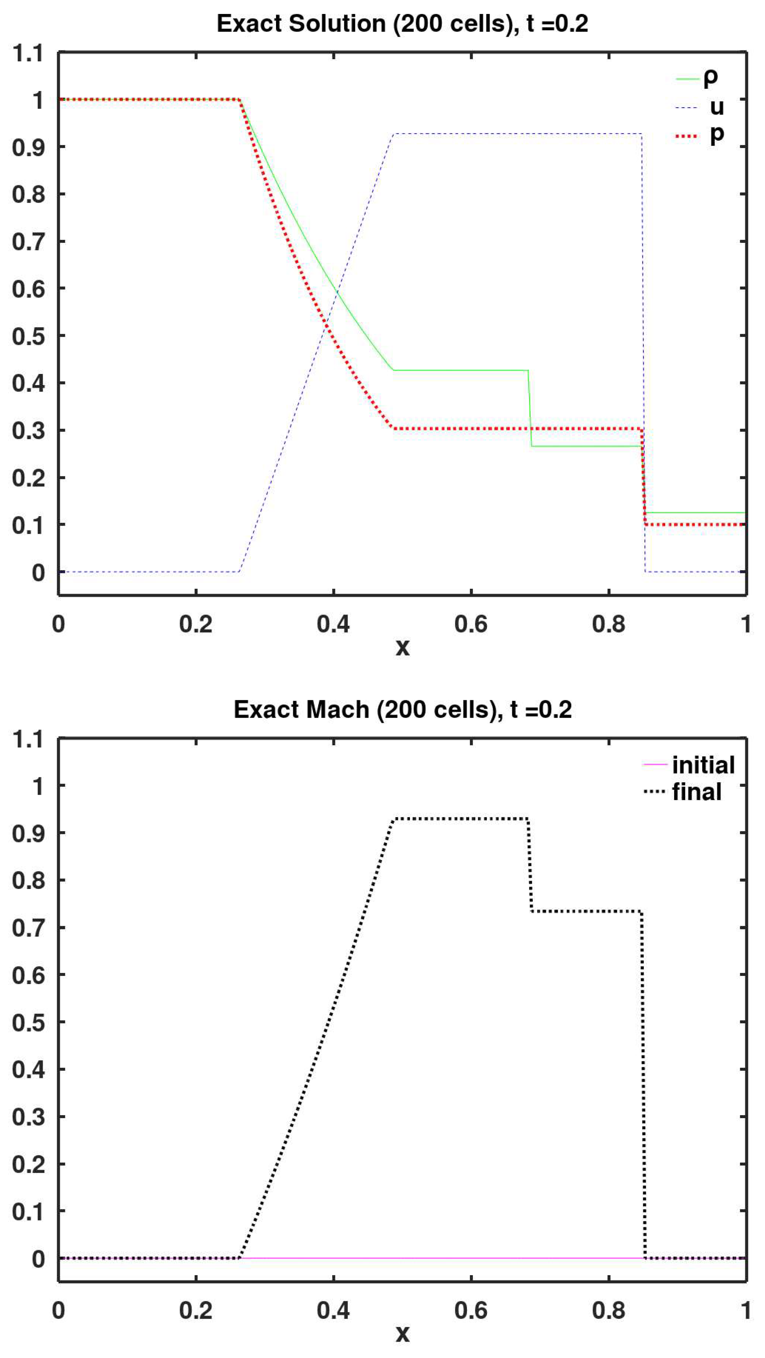
Figure 5.
Published exact and calculated final primitive variables (in addition to the specific internal energy) using the Castor solver of compressible hydrodynamic equations for astrophysical flows. The exact solution is in a red solid line, whereas the calculated one is in markers (with courteous permission from Dr. Michael Zingale, Associate Professor, Stony Brook University, a member of the Castro team of core developers). The problem domain is three-dimensional. Source: https://amrex-astro.github.io/Castro/docs/Verification.html#sods-problem-and-other-shock-tube-problems.
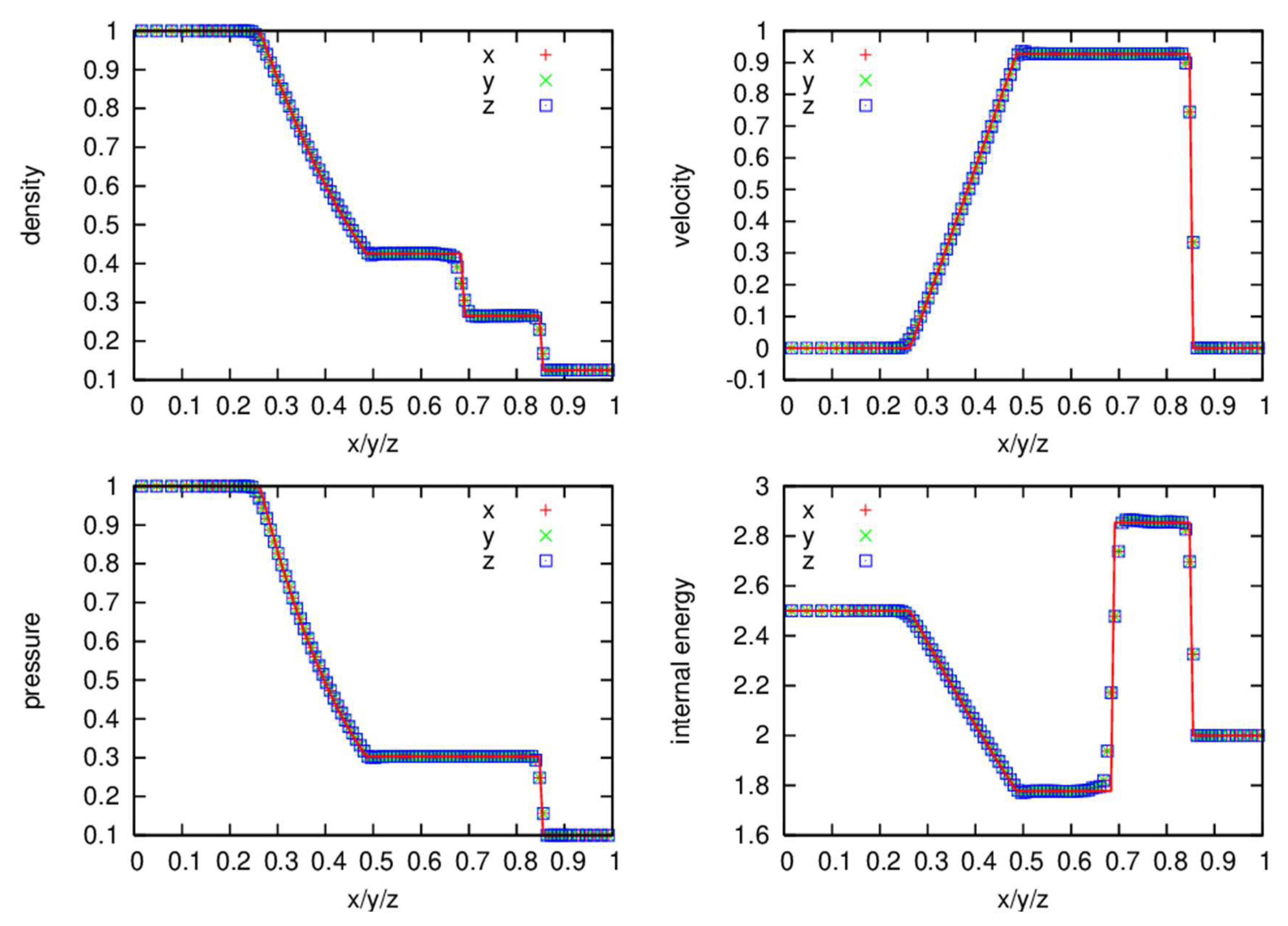
Figure 4.
Illustration of interpolation/extrapolation process to obtain the left and right face values of a generic variable using the MUSCL scheme.
Figure 4.
Illustration of interpolation/extrapolation process to obtain the left and right face values of a generic variable using the MUSCL scheme.
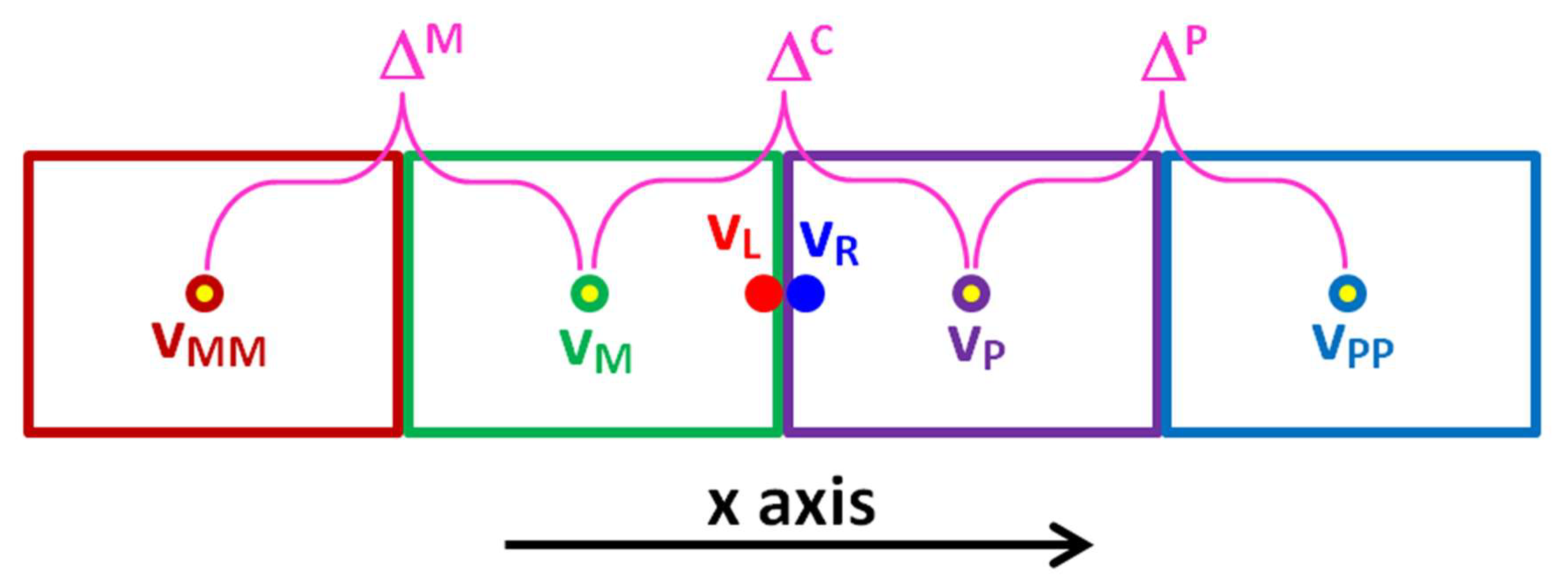

Table 1.
Initial left and right states in the Sod problem.
| Primitive variable | ||||||
|---|---|---|---|---|---|---|
| Density | Velocity | Pressure | Speed of sound | Specific internal energy | Specific enthalpy | |
| Left state | 1.0 | 0.0 | 1.0 | 1.18322 | 2.5 | 3.5 |
| Right state | 0.125 | 0.0 | 0.1 | 1.05830 | 2.0 | 2.8 |
Table 2.
Calculated properties of the three waves in the exact solution of the Sod problem.
| Wave type | Property | Value | Remarks |
|---|---|---|---|
| Expansion Fan | Velocity of the head | -1.18322 | The negative signs mean going left |
| Velocity of the tail | -0.07027 | ||
| Contact Discontinuity | Velocity | 0.92745 | The gas on both sides has the same velocity |
| Pressure | 0.30313 | Equal pressures on both sides of the contact wave | |
| Left density | 0.42632 |
= 0.99773 = 1.77760 = 2.48864 |
|
| Right density | 0.26557 |
= 1.26411 = 2.85354 = 3.99496 |
|
| Shock Wave | Velocity | 1.75216 | |
| Shock-relative Mach number of unshocked gas | 1.65563 | Must have a supersonic regime (Mach > 1) and a subsonic regime (Mach < 1) in this order to avoid a universal entropy decrease, which violates the second law of thermodynamics (Kuznetsov, 2000) | |
| Shock-relative Mach number of shocked gas | 0.65240 |
Table 3.
Comparison of the RMSE (root-mean-square error) for each of the three primitive variables and the Mach number, corresponding to the flux methods used here.
Table 3.
Comparison of the RMSE (root-mean-square error) for each of the three primitive variables and the Mach number, corresponding to the flux methods used here.
| Index | Flux method (short name) | RMSE (density) | RMSE (velocity) | RMSE (pressure) | RMSE (Mach) |
|---|---|---|---|---|---|
| 1 | Riemann | 0.00798 | 0.02345 | 0.00811 | 0.02160 |
| 2 | Roe | 0.00777 | 0.02216 | 0.00796 | 0.02052 |
| 3 | KNP | 0.00829 | 0.02423 | 0.00807 | 0.02245 |
| 4 | KT | 0.00889 | 0.02519 | 0.00760 | 0.02374 |
| 5 | SW | 0.03281 | 0.11764 | 0.02876 | 0.09749 |
| 6 | vanLeer | 0.00767 | 0.02624 | 0.00758 | 0.02405 |
| 7 | AUSM | 0.01127 | 0.02595 | 0.01315 | 0.02462 |
| 8 | AUSM+ | 0.00947 | 0.02380 | 0.01040 | 0.02284 |
| 9 | AUSM+-up | 0.00748 | 0.03047 | 0.00695 | 0.02795 |
| 10 | AUFS | 0.00835 | 0.02121 | 0.00891 | 0.01983 |
| 11 | HLL-Davis1 | 0.00818 | 0.02184 | 0.00788 | 0.02063 |
| 12 | HLL-Davis2 | 0.00829 | 0.02423 | 0.00807 | 0.02245 |
| 13 | HLL-Roe | 0.00821 | 0.02213 | 0.00796 | 0.02075 |
| 14 | HLL-Einfelt | 0.00821 | 0.02219 | 0.00797 | 0.02079 |
| 15 | HLL-pBased | 0.00824 | 0.02312 | 0.00799 | 0.02161 |
| 16 | HLLC-Davis1 | 0.00793 | 0.02234 | 0.00805 | 0.02076 |
| 17 | HLLC-Davis2 | 0.00790 | 0.02381 | 0.00800 | 0.02200 |
| 18 | HLLC-Roe | 0.00787 | 0.02209 | 0.00794 | 0.02054 |
| 19 | HLLC-Einfelt | 0.00788 | 0.02213 | 0.00794 | 0.02058 |
| 20 | HLLC-pBased | 0.00786 | 0.02324 | 0.00797 | 0.02149 |
| 21 | LF | 0.04383 | 0.11586 | 0.05071 | 0.11419 |
| 22 | Rusanov | 0.00889 | 0.02519 | 0.00760 | 0.02374 |
Table 4.
Comparison of the aggregate RMSE (sum over those for the density, velocity, pressure, and Mach number) for each of the flux method used here. Values are ordered from smallest (best) to largest (worst).
Table 4.
Comparison of the aggregate RMSE (sum over those for the density, velocity, pressure, and Mach number) for each of the flux method used here. Values are ordered from smallest (best) to largest (worst).
| Index | Flux method | RMSE (aggregate) |
|---|---|---|
| 10 | AUFS | 0.05830 |
| 2 | Roe | 0.05841 |
| 18 | HLLC-Roe | 0.05844 |
| 11 | HLL-Davis1 | 0.05853 |
| 19 | HLLC-Einfelt | 0.05853 |
| 13 | HLL-Roe | 0.05905 |
| 16 | HLLC-Davis1 | 0.05908 |
| 14 | HLL-Einfelt | 0.05916 |
| 20 | HLLC-pBased | 0.06056 |
| 15 | HLL-pBased | 0.06096 |
| 1 | Riemann | 0.06114 |
| 17 | HLLC-Davis2 | 0.06171 |
| 3 | KNP | 0.06304 |
| 12 | HLL-Davis2 | 0.06304 |
| 4 | KT | 0.06542 |
| 22 | Rusanov | 0.06542 |
| 6 | vanLeer | 0.06554 |
| 8 | AUSM+ | 0.06651 |
| 9 | AUSM+-up | 0.07285 |
| 7 | AUSM | 0.07499 |
| 5 | SW | 0.27670 |
| 21 | LF | 0.32459 |
Table 5.
Comparison of the elapsed time (the runtime) for each of the flux method used here. Values are ordered from smallest (best) to largest (worst).
Table 5.
Comparison of the elapsed time (the runtime) for each of the flux method used here. Values are ordered from smallest (best) to largest (worst).
| Index | Flux method | Elapsed time (in seconds) | Percentage Increase of time (relative to the shortest one) |
|---|---|---|---|
| 5 | SW | 41.13235 | 0.0% |
| 7 | AUSM | 41.54838 | 1.0% |
| 3 | KNP | 41.68739 | 1.3% |
| 4 | KT | 41.69439 | 1.4% |
| 10 | AUFS | 41.90940 | 1.9% |
| 6 | vanLeer | 41.91540 | 1.9% |
| 17 | HLLC-Davis2 | 42.30342 | 2.8% |
| 11 | HLL-Davis1 | 42.42343 | 3.1% |
| 22 | Rusanov | 42.56944 | 3.5% |
| 8 | AUSM+ | 42.78445 | 4.0% |
| 12 | HLL-Davis2 | 42.85645 | 4.2% |
| 16 | HLLC-Davis1 | 42.97146 | 4.5% |
| 13 | HLL-Roe | 43.10346 | 4.8% |
| 15 | HLL-pBased | 43.16347 | 4.9% |
| 14 | HLL-Einfelt | 43.36448 | 5.4% |
| 18 | HLLC-Roe | 43.80651 | 6.5% |
| 20 | HLLC-pBased | 43.82451 | 6.5% |
| 9 | AUSM+-up | 44.00052 | 7.0% |
| 2 | Roe | 44.67956 | 8.6% |
| 19 | HLLC-Einfelt | 44.76256 | 8.8% |
| 21 | LF | 45.50260 | 10.6% |
| 1 | Riemann | 46.49466 | 13.0% |
Disclaimer/Publisher’s Note: The statements, opinions and data contained in all publications are solely those of the individual author(s) and contributor(s) and not of MDPI and/or the editor(s). MDPI and/or the editor(s) disclaim responsibility for any injury to people or property resulting from any ideas, methods, instructions or products referred to in the content. |
© 2025 by the authors. Licensee MDPI, Basel, Switzerland. This article is an open access article distributed under the terms and conditions of the Creative Commons Attribution (CC BY) license (http://creativecommons.org/licenses/by/4.0/).
Copyright: This open access article is published under a Creative Commons CC BY 4.0 license, which permit the free download, distribution, and reuse, provided that the author and preprint are cited in any reuse.


