Submitted:
05 February 2025
Posted:
07 February 2025
You are already at the latest version
Abstract
The rapid advancements in artificial intelligence (AI) have significantly transformed the fields of machine learning, deep learning, and robotics. This comprehensive review aims to provide an in-depth survey of the current state of AI models, focusing on machine learning, deep learning, large language models (LLMs), and multimodal models. Special emphasis is placed on explainable AI (XAI) techniques, which are crucial for fostering transparency, trust, and collaboration between humans and robots. We begin by categorizing and summarizing the various machine learning and deep learning models, including supervised, unsupervised, ensemble, and reinforcement learning approaches. We also explore the latest developments in LLMs and multimodal models, highlighting their applications and potential in various domains. The core of this review delves into XAI techniques, discussing both model-specific and model-agnostic methods. We examine global and local explainability, intrinsic and post-hoc explanations, and their relevance to different AI applications. Moreover, we extend our discussion to explainable AI in robotics, covering topics such as human-robot interaction, autonomous robot transparency, interpretable learning for robotic control, collaborative robotics, safety, adaptability, and ethical considerations. By integrating these diverse perspectives, this review aims to provide a holistic understanding of the interplay between advanced AI models and explainability. Our goal is to highlight the importance of transparent and interpretable AI systems in enhancing the functionality and reliability of robotic applications, ultimately contributing to the development of trustworthy AI technologies.
Keywords:
Artificial Intelligence
; Machine Learning
; Explainable AI
; MultiModal Transformers
; Deep Learning
1. Introduction
Artificial Intelligence (AI) has become a transformative force in the modern era, revolutionizing industries such as healthcare, finance, education, and transportation. AI, broadly defined as the capability of machines to simulate human intelligence, encompasses a wide array of methodologies and applications. The global AI market is projected to grow from USD 136.6 billion in 2022 to USD 1,811.8 billion by 2030, with a compound annual growth rate (CAGR) of 38.1%, [1]. At the core of this revolution lie Machine Learning (ML) and Deep Learning (DL), which provide data-driven frameworks to enable systems to learn, reason, and make decisions as depicted in Figure 1.
Machine Learning (ML), a subset of AI, is centered on developing algorithms that allow systems to learn patterns and make predictions from data. ML models are broadly categorized into supervised learning, unsupervised learning, and reinforcement learning. Supervised learning, with methods like Linear Regression [2], Logistic Regression [3], and Decision Trees [4], focuses on predicting labeled outcomes. Unsupervised learning methods, such as K-Means Clustering [5] and Principal Component Analysis (PCA) [6], discover hidden structures in data. Reinforcement learning techniques, such as Q-Learning [7] and Deep Q-Networks (DQN) [8], are employed in sequential decision-making tasks like robotics and autonomous systems.
Deep Learning (DL), a specialized subset of ML, is inspired by the structure and function of the human brain. Deep neural networks, such as Convolutional Neural Networks (CNNs) [9] and Recurrent Neural Networks (RNNs) [10], have demonstrated unprecedented performance in complex tasks like image recognition, natural language processing, and speech synthesis. Landmark architectures, including AlexNet [11], ResNet [12], and Transformers [13], have redefined state-of-the-art in DL by enabling scalable and efficient learning from vast datasets.
Explainable AI (EAI) has emerged as a critical component of AI research, addressing the need for transparency, fairness, and accountability in AI systems. As AI becomes increasingly integrated into high-stakes domains, the ability to explain and interpret model decisions has become paramount. Techniques such as Local Interpretable Model-Agnostic Explanations (LIME) [14] and SHAP (SHapley Additive exPlanations) [15] are widely used to enhance the interpretability of complex models, particularly in sensitive applications like healthcare diagnostics and financial risk assessment.
Robotics represents another domain profoundly influenced by AI. Modern robots leverage ML and DL techniques for tasks ranging from perception and navigation to manipulation and human-robot interaction. Reinforcement learning plays a pivotal role in enabling robots to learn adaptive behaviors in dynamic environments. Multi-modal learning, exemplified by models like CLIP [16] and Flamingo [17], has further expanded the capabilities of robotics, allowing machines to integrate visual and textual information seamlessly.
The convergence of AI subfields is driving innovation across domains, making AI an indispensable tool for addressing global challenges. From enabling autonomous vehicles to optimizing supply chains and advancing personalized medicine, the impact of AI is profound and far-reaching. This paper delves into the theoretical foundations, architectures, and applications of AI, ML, DL, EAI, and Robotics, highlighting their interconnections and potential to shape the future.
1.1. Organization of the Paper
The rest of the paper is organized as follows. Section 2 discusses the foundations of Machine Learning (ML), including key techniques in supervised, unsupervised, and reinforcement learning. Section 3 delves into Deep Learning (DL), exploring prominent architectures such as Convolutional Neural Networks (CNNs), Recurrent Neural Networks (RNNs), and Transformers. Section 4 introduces Explainable AI (EAI) and its importance in enhancing transparency and trust in AI systems. Section 5 examines the integration of AI in Robotics, highlighting applications in perception, control, and human-robot interaction. Finally, Section 6 concludes the paper with a summary of findings and a discussion on future research directions in AI and its subfields.
2. Machine Learning Models
Machine Learning (ML) is a subset of artificial intelligence that focuses on developing algorithms capable of learning from data and making predictions or decisions without explicit programming. ML models can be broadly categorized into supervised, unsupervised, and reinforcement learning paradigms, each tailored to address specific types of problems. Supervised learning involves training models on labeled data to predict outcomes, while unsupervised learning identifies hidden patterns or structures in unlabeled data. Reinforcement learning, on the other hand, enables agents to learn optimal strategies by interacting with an environment. This section explores key machine learning models, highlighting their architectures, applications, and strengths in tackling diverse challenges.
The image illustrates a comparative overview of processes in machine learning, deep learning, and transformer-based large language models (LLMs). The top section represents the general machine learning process, which begins with data (inputs and targets), followed by the model creation (algorithm and parameters), training (using loss functions and optimization), evaluation (based on metrics), and finally deployment. The middle section details the deep learning process, which involves normalized input data being processed through layers (e.g., convolutional, ReLU, and pooling), training using backpropagation and optimization algorithms (e.g., Adam), evaluation metrics (accuracy and loss), and deployment. The bottom section focuses on transformers for large language models, starting with tokenized and embedded input data, passed through transformer layers (incorporating attention mechanisms), trained with methods like masked language modeling and cross-entropy loss, evaluated using metrics such as perplexity and F1 score, and ending with deployment. These processes highlight the increasing complexity and specialization as we progress from traditional machine learning to advanced deep learning and transformer-based approaches (see Figure 2).
2.1. Supervised Learning
Supervised learning is a machine learning paradigm where models are trained on labeled datasets, enabling them to learn the mapping between inputs and corresponding outputs. By minimizing prediction errors on training data, supervised learning models generalize to unseen data for tasks such as classification and regression. Techniques like Linear Regression, Logistic Regression, Decision Trees, and Support Vector Machines have become foundational in solving problems ranging from medical diagnostics to financial forecasting. This subsection delves into key supervised learning models, discussing their mechanisms and practical applications.
2.1.1. Linear Regression
Linear Regression is a foundational supervised learning technique that models the relationship between a dependent variable y and one or more independent variables x using a linear equation[2]. The model assumes a linear relationship between the variables, making it suitable for predicting numerical outcomes. It can be expressed mathematically as:
where y is the predicted value, represents the independent variables, are the coefficients of the model, and is the error term accounting for the deviation of the actual data from the model prediction.
Applications: Linear Regression is widely used in various domains, including finance for predicting stock prices, economics for demand forecasting, biology for growth predictions, and marketing for sales forecasting. It provides interpretable results, making it valuable in fields where understanding the impact of each variable is crucial.
Advantages: The simplicity of Linear Regression enables easy interpretation of relationships, providing clear insights into variable dependencies. It is computationally efficient, especially for problems with a small number of features, and serves as a baseline for more complex models.
Drawbacks: Linear Regression has several limitations. The assumption of a linear relationship does not hold for many real-world scenarios, leading to inaccuracies. It is also sensitive to outliers, which can significantly distort the model’s predictions. Additionally, the presence of multicollinearity (high correlation between independent variables) can affect the reliability of the coefficient estimates.
Mathematical Foundation: To estimate the coefficients , the model minimizes the Mean Squared Error (MSE) between the predicted and actual values. This optimization problem is defined as:
where n is the number of data points, is the actual value, and is the predicted value. The solution involves calculating the best-fit line by deriving the partial derivatives of MSE with respect to each , setting them to zero, and solving the resulting equations.
Linear Regression remains an essential technique in machine learning due to its simplicity, interpretability, and foundational value in understanding more complex models.
2.1.2. Logistic Regression
Logistic Regression is a widely used supervised learning algorithm for binary classification tasks, where the goal is to predict one of two possible outcomes. Unlike Linear Regression, which is used for continuous target variables, Logistic Regression models the probability of a categorical outcome by mapping input features to a probability value between 0 and 1[3]. This is achieved through the logistic (sigmoid) function, defined as:
where is the probability that the target variable y belongs to class 1, represents the independent features, and are the coefficients estimated by the model. The model fits the data by maximizing the likelihood function, which finds the coefficients that make the observed values most probable.
Logistic Regression is extensively used in fields like healthcare, for predicting the likelihood of a disease, in finance for credit scoring, and in marketing for customer retention prediction. Its probabilistic interpretation and straightforward implementation make it popular, especially in cases where interpretability is essential. However, Logistic Regression assumes a linear relationship between the independent variables and the log odds of the dependent variable, which may not be appropriate for complex relationships. Additionally, it can be sensitive to multicollinearity and may require regularization for datasets with many features to prevent overfitting. Despite these limitations, Logistic Regression remains a reliable, efficient baseline for binary classification, especially in cases with balanced classes and limited feature interactions.
2.1.3. Decision Trees
Decision Trees are a versatile and interpretable supervised learning technique used for both classification and regression tasks[4]. The model operates by recursively splitting the data into subsets based on feature values, constructing a tree-like structure where each node represents a decision point on an attribute. Starting at the root, the tree partitions data at each node using criteria like Gini impurity or information gain (for classification) and mean squared error (for regression). This recursive partitioning continues until reaching leaf nodes, where each leaf represents a class label or a predicted value.
The strength of Decision Trees lies in their simplicity and interpretability, as the resulting model is a clear set of rules derived from the data, making them particularly useful in areas like medical diagnostics, credit scoring, and decision-making systems where transparency is crucial. However, they are prone to overfitting, especially when the tree grows too complex by capturing noise in the data. Techniques like pruning and setting maximum depths can mitigate overfitting, and ensemble methods, such as Random Forests, further improve their robustness. Despite these challenges, Decision Trees remain a fundamental and intuitive model in machine learning, providing a foundation for understanding more complex ensemble methods.
2.1.4. Support Vector Machines (SVM)
Support Vector Machines (SVM) are a powerful supervised learning model used primarily for classification but also applicable to regression tasks. SVM works by finding the optimal hyperplane that maximally separates data points of different classes in a high-dimensional space. The objective is to create a decision boundary with the maximum possible margin between the nearest data points of each class, known as support vectors[18]. Mathematically, for a linear SVM, this is achieved by minimizing the following objective function:
subject to the constraint , where represents the weight vector, b is the bias term, denotes the class label, and represents the feature vector of each data point.
For cases where the data is not linearly separable, SVM employs a kernel trick, mapping data into a higher-dimensional space where a linear separation is feasible. Common kernels include the radial basis function (RBF) and polynomial kernels, which allow SVM to capture complex patterns in data. SVM is widely used in fields such as image recognition, bioinformatics, and text categorization, where precise and robust classification is essential. While SVMs are effective, especially with smaller datasets and clear margins between classes, they can be computationally intensive for large datasets and may not perform well in highly overlapping or noisy data scenarios. Furthermore, the choice of kernel and tuning of hyperparameters significantly affect the model’s performance, requiring careful experimentation.
2.1.5. K-Nearest Neighbors (KNN)
K-Nearest Neighbors (KNN) is a simple yet effective non-parametric supervised learning algorithm used for both classification and regression tasks[19]. The core idea behind KNN is to classify a new data point based on the majority label of its k nearest neighbors, where k is a user-defined parameter. For regression tasks, KNN predicts the outcome as the average of the values of the k nearest neighbors. The distance between data points is typically measured using metrics such as Euclidean, Manhattan, or Minkowski distance.
KNN is widely used in fields such as recommendation systems, image recognition, and anomaly detection due to its simplicity and flexibility. It requires no training phase, making it particularly suited for applications where training costs need to be minimized or when working with small datasets. However, KNN’s performance can degrade with high-dimensional data due to the curse of dimensionality, as distance metrics become less informative. Additionally, KNN can be computationally expensive for large datasets since it must calculate the distance to all data points in the training set to make predictions. Techniques like dimensionality reduction and approximate nearest neighbors can help mitigate these issues, enhancing KNN’s practicality in larger or more complex datasets.
2.1.6. Naive Bayes
Naive Bayes is a probabilistic supervised learning algorithm based on Bayes’ Theorem, commonly used for classification tasks[20]. It operates under the “naive” assumption that all features are independent of each other, which simplifies calculations and makes the model computationally efficient. Bayes’ Theorem is expressed as:
where is the posterior probability of the class y given the feature vector X, is the likelihood of observing the feature vector X given the class y, is the prior probability of the class, and is the marginal probability of the feature vector.
Naive Bayes is particularly effective in applications like text classification, spam detection, and sentiment analysis, where the independence assumption often holds approximately and computation speed is essential. Despite its simplicity, Naive Bayes performs surprisingly well in many real-world scenarios, especially when dealing with high-dimensional data. However, its reliance on the independence assumption can limit its accuracy in cases where features are strongly correlated, making it less suitable for datasets with high inter-feature dependencies. To address this, variations like Multinomial and Gaussian Naive Bayes have been developed, tailored to different types of data distributions.
2.1.7. Ridge Regression
Ridge Regression is a linear regression technique that addresses multicollinearity in datasets by introducing a regularization term[21]. This method modifies the ordinary least squares (OLS) regression by adding a penalty to the loss function, which helps prevent overfitting and improves the stability of the model’s coefficients. The objective function for Ridge Regression is given by:
where represents the actual target values, represents the predicted values, are the coefficients, and is the regularization parameter that controls the penalty’s strength. When , Ridge Regression reduces to ordinary least squares, while larger values of shrink the coefficients toward zero.
Ridge Regression is particularly useful in cases with multicollinearity or when the number of predictors exceeds the number of observations, such as in gene expression data or text data with many features. By reducing the model’s complexity, Ridge Regression improves generalization, although it may still retain all features without completely zeroing out any coefficients. One limitation of Ridge Regression is that it does not perform feature selection, unlike Lasso Regression, which can set some coefficients exactly to zero. Nevertheless, Ridge Regression remains a robust technique for handling linear relationships in high-dimensional datasets.
2.1.8. Lasso Regression
Lasso Regression, short for Least Absolute Shrinkage and Selection Operator, is a linear regression technique that incorporates a regularization term to prevent overfitting and enhance model interpretability by performing feature selection [22]. Unlike Ridge Regression, which penalizes the sum of squared coefficients, Lasso Regression adds an penalty, which is the sum of the absolute values of the coefficients. The objective function for Lasso Regression is given by:
where represents the actual target values, represents the predicted values, are the coefficients, and is the regularization parameter controlling the strength of the penalty. As increases, some coefficients are forced to exactly zero, effectively selecting a subset of features and discarding the rest.
Lasso Regression is widely used in fields such as bioinformatics, economics, and high-dimensional datasets, where interpretability and feature selection are critical. By setting some coefficients to zero, Lasso provides a sparse model, making it particularly useful for datasets with many irrelevant features. However, in cases where features are highly correlated, Lasso may arbitrarily select one feature and ignore others, potentially impacting model stability. Despite this limitation, Lasso Regression remains a powerful tool for creating simpler, more interpretable models in high-dimensional data environments.
2.1.9. Elastic Net
Elastic Net is a regularized linear regression technique that combines the penalties of both Ridge and Lasso Regression [23]. By introducing both and penalties, Elastic Net addresses the limitations of each individual method, making it effective in scenarios with correlated features or high-dimensional data. The objective function for Elastic Net is given by:
where represents the actual target values, represents the predicted values, are the coefficients, and and are regularization parameters that control the strength of the and penalties, respectively. The inclusion of the penalty allows for feature selection by setting some coefficients to zero, while the penalty helps to stabilize the model in cases of multicollinearity.
Elastic Net is particularly useful in situations where there are multiple correlated features, as it tends to select groups of correlated variables together. This makes it suitable for applications such as genomics, where features (genes) are often highly correlated. The flexibility of Elastic Net to combine both types of regularization makes it robust for high-dimensional datasets. However, tuning both and adds complexity to the model training process, requiring cross-validation to find the optimal balance between the two penalties. Despite this, Elastic Net is a powerful alternative to Ridge and Lasso when dealing with complex, high-dimensional data structures.
2.1.10. Linear Discriminant Analysis (LDA)
Linear Discriminant Analysis (LDA) is a supervised learning algorithm primarily used for classification tasks [24]. LDA aims to find a linear combination of features that best separates data points from different classes. By maximizing the ratio of between-class variance to within-class variance, LDA identifies a projection that enhances class separability. Mathematically, this is achieved by solving an eigenvalue problem to find the direction vectors, known as discriminant components, that maximize class separation.
The model assumes that each class follows a Gaussian distribution with a shared covariance matrix, making it particularly effective when this assumption holds. LDA projects data onto a lower-dimensional space (typically one less than the number of classes), where the separation between classes is maximized. This makes it especially useful in applications such as face recognition, bioinformatics, and medical diagnosis, where dimensionality reduction and classification are key.
LDA’s strength lies in its interpretability and ability to handle linearly separable classes efficiently. However, its performance diminishes when classes are not linearly separable or when the Gaussian assumption does not hold, as it assumes homoscedasticity (equal variance across classes). Despite these limitations, LDA remains a powerful tool for classification and dimensionality reduction, particularly in settings where the Gaussian assumption is reasonable.
2.1.11. Quadratic Discriminant Analysis (QDA)
Quadratic Discriminant Analysis (QDA) is an extension of Linear Discriminant Analysis (LDA) that relaxes the assumption of a shared covariance matrix across classes, allowing each class to have its own covariance matrix [25]. This flexibility enables QDA to model more complex, non-linear decision boundaries between classes, making it effective in scenarios where class distributions differ significantly in variance and orientation. The decision boundary formed by QDA is quadratic, hence the name.
QDA works by assuming that each class follows a Gaussian distribution, with its own mean vector and covariance matrix. Given these parameters, QDA calculates the posterior probability of a data point belonging to each class and assigns it to the class with the highest probability. This approach is valuable in fields like image recognition, medical diagnostics, and finance, where different groups may exhibit distinct distribution patterns.
While QDA provides more flexibility than LDA, it also has a higher risk of overfitting, especially when the number of features is large relative to the number of observations. This is because each class requires its own covariance matrix, which increases the number of parameters to estimate. Consequently, QDA is most effective when there is sufficient data to robustly estimate the covariance matrices for each class. Despite this drawback, QDA is a powerful classification tool when dealing with data that exhibit non-linear class boundaries.
2.1.12. Bayesian Networks
Bayesian Networks, also known as Belief Networks or Bayes Nets, are probabilistic graphical models that represent a set of variables and their conditional dependencies through a directed acyclic graph (DAG) [26]. Each node in the graph corresponds to a random variable, and the edges denote conditional dependencies between variables. Bayesian Networks leverage Bayes’ Theorem to compute the probability of a variable given the values of its parent nodes, allowing them to model complex probabilistic relationships in uncertain environments.
Formally, a Bayesian Network defines the joint probability distribution over a set of variables as the product of conditional probabilities:
where denotes the set of parent nodes of in the DAG. This factorization provides computational efficiency, as it reduces the complexity of calculating joint probabilities across multiple variables.
Bayesian Networks are widely applied in fields such as medical diagnosis, natural language processing, and risk assessment, where understanding conditional dependencies is crucial. They provide interpretable structures that facilitate decision-making under uncertainty. However, constructing and training Bayesian Networks can be computationally intensive, particularly for large networks with many dependencies, and they require careful estimation of conditional probabilities. Despite these challenges, Bayesian Networks remain a valuable tool for modeling probabilistic relationships and handling complex, uncertain datasets.
2.1.13. Least Squares Support Vector Machines (LS-SVM)
Least Squares Support Vector Machines (LS-SVM) are a modified version of traditional Support Vector Machines (SVM) that simplify the optimization problem by reformulating it as a set of linear equations [27]. Unlike standard SVM, which minimizes a hinge loss function, LS-SVM minimizes a sum of squared errors. This change in the objective function allows LS-SVM to use a least-squares cost function, which leads to easier implementation and computational efficiency.
The objective function for LS-SVM can be written as:
subject to the equality constraints , where is the weight vector, b is the bias term, is a regularization parameter that controls the trade-off between the margin and the classification error, are the error terms, and is the mapping to a higher-dimensional space. The solution to this optimization problem involves solving a set of linear equations instead of a quadratic programming problem, as in traditional SVM, resulting in faster computation.
LS-SVMs are applicable in classification and regression tasks and are used in areas such as signal processing, financial prediction, and bioinformatics, where high-dimensional or nonlinear data structures are common. While LS-SVMs offer computational advantages and ease of implementation, they may be more sensitive to outliers due to the use of squared errors. Despite this limitation, LS-SVM provides a valuable alternative to traditional SVMs, especially in scenarios requiring fast and efficient computation.
2.2. Ensemble Learning
Ensemble learning is a machine learning technique that combines the predictions of multiple models to improve overall accuracy and robustness compared to individual models. By aggregating diverse models, ensemble methods reduce the likelihood of errors, enhance generalization, and mitigate issues such as overfitting. Ensemble learning approaches can be categorized primarily into two types: bagging and boosting. In bagging, models are trained independently on random subsets of the data, with predictions averaged or voted upon to produce a final output. Boosting, on the other hand, involves training models sequentially, where each model attempts to correct the errors of its predecessor.
Ensemble learning is widely used in applications requiring high predictive accuracy, such as finance, healthcare, and image classification, as it leverages the strengths of multiple models to achieve better performance than individual methods. Techniques like Random Forest, Gradient Boosting, and AdaBoost are popular ensemble methods, each providing unique advantages and trade-offs in terms of computational efficiency, interpretability, and performance.
2.2.1. Random Forest
Random Forest is an ensemble learning method that builds multiple decision trees and combines their outputs to improve accuracy and robustness in classification and regression tasks[28]. Developed by aggregating predictions from a collection (or "forest") of individual decision trees, Random Forest introduces two main sources of randomness: bootstrapping and feature selection. Each tree is trained on a random subset of the data with replacement (bootstrapping), and at each split, a random subset of features is considered, ensuring diversity among the trees. The final prediction is obtained by averaging the outputs (in regression) or using a majority vote (in classification) from all trees.

Table 1.
Comparison of Supervised Machine Learning Algorithms.
| Name of the Algorithm | Popularity | Mathematical Representation | Short Description | Benefits | Problems | What is Different than Other Classifier | Overall Performance by Other Researchers |
|---|---|---|---|---|---|---|---|
| Linear Regression | High | A statistical method for modeling the relationship between a dependent variable and one or more independent variables. | Simple to implement and interpret, good for linear relationships. | Not suitable for non-linear data, sensitive to outliers. | Directly models the relationship between variables. | Effective for linear relationships, widely used in many fields. | |
| Logistic Regression | High | Used for binary classification, predicts the probability of the default class. | Probabilistic framework, interpretable coefficients. | Assumes linear relationship between variables and log-odds, not suitable for non-linear problems. | Outputs probabilities, not just class labels. | Widely used for binary classification tasks, performs well with linear decision boundaries. | |
| Decision Trees | High | Tree-like model for decision making, splits data into subsets based on feature values. | Easy to interpret and visualize, handles non-linear relationships. | Prone to overfitting, sensitive to noisy data. | Simple and interpretable model structure. | Effective for both classification and regression tasks, popular in many applications. | |
| Support Vector Machines (SVM) | High | Finds the hyperplane that best separates the classes in the feature space. | Effective in high-dimensional spaces, robust to overfitting. | Computationally intensive, requires careful parameter tuning. | Maximizes margin between classes. | High accuracy in various classification tasks, especially with clear margin of separation. | |
| K-Nearest Neighbors (KNN) | Moderate | Classifies a sample based on the majority class among its k-nearest neighbors. | Simple and intuitive, no training phase. | Computationally expensive during prediction, sensitive to irrelevant features. | Non-parametric, makes few assumptions about the data. | Performs well with sufficient and relevant data, used in various domains. | |
| Naive Bayes | High | Probabilistic classifier based on Bayes’ theorem, assumes feature independence. | Simple and fast, works well with high-dimensional data. | Assumes independence among features, which is often not true. | Works well with small data sets and high-dimensional data. | Effective in text classification and spam detection, performs surprisingly well despite simplicity. | |
| Ridge Regression | Moderate | Extension of linear regression with L2 regularization to prevent overfitting. | Reduces model complexity, handles multicollinearity. | Can still be affected by outliers. | Regularization helps prevent overfitting. | Useful in situations with many correlated features, often performs better than linear regression. | |
| Lasso Regression | Moderate | Linear regression with L1 regularization, encourages sparsity in coefficients. | Performs feature selection, reduces model complexity. | Can discard important features if not tuned properly. | Can perform automatic feature selection. | Effective for datasets with many features, especially when some are irrelevant. | |
| Elastic Net | Moderate | Combines L1 and L2 regularization, balances between ridge and lasso regression. | Handles multicollinearity, performs feature selection. | Complex tuning process due to two regularization parameters. | Combines benefits of ridge and lasso regression. | Often outperforms both ridge and lasso when dealing with correlated features. | |
| Linear Discriminant Analysis (LDA) | High | Finds a linear combination of features that best separates two or more classes. | Simple and computationally efficient, works well with normally distributed data. | Assumes normal distribution of features, equal covariance among classes. | Maximizes separation between classes. | Effective for low-dimensional data, commonly used for classification problems. | |
| Quadratic Discriminant Analysis (QDA) | Moderate | Extension of LDA, allows for different covariance matrices for each class. | More flexible than LDA, can model more complex boundaries. | Requires more data to estimate separate covariance matrices accurately. | Allows for quadratic decision boundaries. | Effective for datasets where classes have different covariance structures. | |
| Bayesian Networks | Moderate | Probabilistic graphical model that represents a set of variables and their conditional dependencies. | Handles uncertainty, incorporates prior knowledge. | Computationally intensive for large networks. | Represents complex relationships between variables. | Effective for reasoning under uncertainty, used in various fields including bioinformatics and diagnostics. | |
| Least Squares Support Vector Machines (LS-SVM) | Moderate | Variant of SVM that uses least squares cost function, simplifies computation. | Computationally efficient, handles non-linear relationships. | Requires careful tuning of parameters. | Simplifies the quadratic optimization problem of SVM. | Comparable performance to traditional SVM, often faster to train. |
Mathematically, if there are T trees in the forest, then for a given input X, the Random Forest output for regression is:
where is the prediction from the t-th tree. For classification, the output is based on the mode of the predictions from each tree.
Random Forest is widely used in applications such as medical diagnosis, finance, and ecology due to its high accuracy, interpretability, and ability to handle large datasets with many features. The method is robust to overfitting because individual trees, though potentially overfitting, average out errors when combined in the ensemble. However, Random Forest can be computationally intensive, especially with many trees and high-dimensional data, and may lose interpretability compared to a single decision tree. Nevertheless, Random Forest remains a popular and powerful tool in machine learning for both classification and regression tasks.
2.2.2. Gradient Boosting Machines (GBM)
Gradient Boosting Machines (GBM) are a powerful ensemble learning method that builds a sequence of decision trees, where each subsequent tree focuses on correcting the errors of its predecessors [29]. GBM combines weak learners—typically shallow trees—into a strong model by using a boosting approach. The model minimizes the loss function iteratively, with each new tree constructed to reduce the residuals (errors) from the previous trees. At each step, the gradient of the loss function with respect to the predictions guides the model’s updates, hence the term “gradient boosting.”
Formally, let be the prediction at the m-th iteration. GBM updates the model by adding a new tree to minimize the loss L, such that:
where is the learning rate that controls the contribution of each tree. Smaller values of generally improve model performance but require more trees, increasing computation time.
GBM is widely used in applications such as financial modeling, customer churn prediction, and ranking tasks, due to its high accuracy and flexibility. While GBM is highly effective, it can be computationally expensive, particularly with large datasets, and may be prone to overfitting if not properly regularized. Techniques like early stopping, tuning the learning rate, and using shallow trees help mitigate overfitting and optimize performance, making GBM a popular choice for tasks requiring predictive precision.
2.2.3. XGBoost
XGBoost, short for Extreme Gradient Boosting, is an advanced implementation of Gradient Boosting that incorporates optimized algorithms to enhance both performance and efficiency. Developed with a focus on computational speed and model accuracy, XGBoost introduces regularization terms to the Gradient Boosting framework, which helps control model complexity and reduce the risk of overfitting [30]. XGBoost uses an additive model where each new tree attempts to correct the errors of the previous trees, similar to traditional Gradient Boosting. However, it optimizes the process by employing advanced techniques such as parallel processing, cache awareness, and out-of-core computation.
In XGBoost, the objective function includes a regularization term that penalizes the complexity of the model:
where L is the loss function measuring the difference between the predicted and actual values, and is the regularization term that penalizes the complexity of each tree . This regularization aids in balancing the model’s bias-variance trade-off, resulting in improved generalization.
XGBoost is extensively used in data science competitions and real-world applications like fraud detection, sales forecasting, and customer churn prediction, owing to its scalability and accuracy on structured datasets. While XGBoost is powerful, it requires careful tuning of hyperparameters (e.g., learning rate, maximum tree depth, regularization terms) to achieve optimal performance. Despite the complexity, XGBoost remains a preferred tool in machine learning due to its robustness and adaptability across a wide range of applications.
2.2.4. LightGBM
LightGBM, short for Light Gradient Boosting Machine, is a gradient boosting framework that builds decision trees efficiently for high-dimensional and large datasets[31]. Unlike traditional gradient boosting methods that grow trees level-wise, LightGBM grows trees leaf-wise, where each iteration splits the leaf with the largest loss reduction. This leaf-wise growth strategy reduces the loss more quickly than level-wise approaches, enhancing both accuracy and speed. Additionally, LightGBM employs histogram-based algorithms and efficient memory usage, making it suitable for large-scale applications.
LightGBM optimizes the objective function by including regularization terms and supports several advanced techniques such as Gradient-based One-Side Sampling (GOSS) and Exclusive Feature Bundling (EFB). GOSS focuses on high-gradient data samples to accelerate training, while EFB combines mutually exclusive features, reducing the feature dimension and enhancing computational efficiency.
LightGBM is widely applied in areas like recommendation systems, ranking tasks, and predictive analytics, where large datasets and high dimensionality require fast and scalable algorithms. Although LightGBM provides high accuracy and computational efficiency, it may overfit on smaller datasets and requires careful tuning, particularly for parameters like learning rate, max depth, and number of leaves. Nevertheless, LightGBM remains a popular choice for high-performance gradient boosting due to its speed and effectiveness.
2.2.5. CatBoost
CatBoost, short for Categorical Boosting, is a gradient boosting framework specifically designed to handle categorical features efficiently without extensive preprocessing[32]. Unlike other boosting algorithms that require categorical variables to be one-hot encoded or label encoded, CatBoost natively supports categorical data, reducing preprocessing time and potential information loss. CatBoost’s unique approach to handling categorical features involves a method called Ordered Boosting, which prevents overfitting by processing the data in a way that reduces target leakage during training.
CatBoost optimizes the objective function similarly to other gradient boosting algorithms but introduces innovations in handling categorical data, supporting symmetric trees, and using robust regularization techniques. The symmetric trees, which maintain balanced splits, allow for faster inference and prevent overfitting by ensuring each split is optimized across the entire tree structure.
CatBoost is particularly effective in applications with many categorical features, such as recommender systems, e-commerce, and finance, where categorical data plays a critical role. It is recognized for delivering high accuracy and requiring less parameter tuning than other gradient boosting methods. However, while CatBoost is user-friendly and efficient with categorical data, it can be more memory-intensive than some other frameworks, especially with very large datasets. Despite this, CatBoost has become popular for tasks involving a mix of numerical and categorical data due to its accuracy and reduced need for feature engineering.
2.3. AdaBoost
AdaBoost, short for Adaptive Boosting, is a popular ensemble learning technique that combines multiple weak learners to form a strong classifier [33]. Typically, AdaBoost uses decision stumps (shallow trees with one split) as its base learners. In each iteration, AdaBoost adjusts the weights of the training samples based on their classification accuracy, emphasizing misclassified samples and reducing the influence of correctly classified ones. This adaptive process allows subsequent learners to focus on difficult cases, resulting in a strong model that effectively handles classification tasks.
Formally, AdaBoost minimizes the exponential loss by iteratively training a series of weak classifiers and updating their weights based on their individual performance. The final prediction is a weighted majority vote of these classifiers, defined as:
where represents the weight of each classifier , determined by its accuracy. The weights increase the influence of more accurate classifiers in the ensemble.
AdaBoost is widely applied in areas such as text classification, image recognition, and fraud detection due to its simplicity and effectiveness in handling binary and multiclass classification problems. However, AdaBoost is sensitive to noisy data and outliers, as it tends to focus heavily on misclassified samples, which can lead to overfitting. Despite this drawback, AdaBoost remains a powerful and interpretable boosting method, particularly useful in scenarios where enhancing weak learners leads to significant performance improvements.
2.3.1. Bagging
Bagging, short for Bootstrap Aggregating, is an ensemble learning technique designed to improve the stability and accuracy of machine learning models by reducing variance [34]. The method involves generating multiple subsets of the training data through bootstrapping—sampling with replacement—and training a separate model on each subset. The predictions from these individual models are then combined, typically by averaging for regression tasks or by majority voting for classification tasks, to produce a final output. This aggregation helps smooth out errors and reduce the tendency to overfit, particularly for high-variance models like decision trees.
Mathematically, if there are T models in the ensemble and represents the prediction from the t-th model, the final prediction for regression is given by:
and for classification, the ensemble prediction is based on the most frequently occurring class label among the individual model predictions.
Bagging is particularly effective in applications like financial modeling, medical diagnosis, and risk assessment, where reducing overfitting and improving model stability is critical. The Random Forest algorithm is a popular implementation of bagging, where each model is a decision tree trained on bootstrapped data with a random selection of features. Although bagging can increase computational requirements due to multiple model training, it remains a valuable approach for enhancing model performance and is widely used in both classification and regression problems.
2.3.2. Stacking
Stacking, or Stacked Generalization, is an ensemble learning technique that combines multiple models to improve predictive performance by training a meta-model to learn the optimal way to combine base model predictions [35]. Unlike Bagging and Boosting, which aggregate predictions through averaging or weighted voting, Stacking involves training a second-level model (the meta-learner) on the predictions of base models, allowing it to learn how to best integrate them for final predictions. This approach enables Stacking to leverage the strengths of various types of models, often resulting in better generalization.
In a typical Stacking framework, the training data is split, and each base model is trained on a subset of the data. Their predictions on a holdout set are then used as features for training the meta-learner. The final output is obtained by applying the meta-learner to the predictions of each base model on the test data. This layered structure allows Stacking to capture complex patterns by integrating diverse perspectives from different base models.
Stacking is commonly used in competitions and real-world applications where maximizing predictive accuracy is crucial, such as in finance, healthcare, and recommendation systems. While Stacking can lead to improved performance, it may increase model complexity and computational costs, as it involves training multiple models and an additional meta-model. Nevertheless, Stacking remains a powerful ensemble method, particularly valuable when combining models with complementary strengths.
2.3.3. Voting Classifier
A Voting Classifier is an ensemble learning technique that combines the predictions of multiple models to produce a final classification result by voting [36]. In this approach, each model in the ensemble independently makes predictions, and the final output is determined by aggregating these predictions, either through hard voting or soft voting. In hard voting, each model casts a single vote for a class label, and the class with the majority of votes is selected. In soft voting, the models provide class probabilities, and the class with the highest average probability is chosen.
The Voting Classifier is particularly useful for improving predictive performance in classification tasks by blending the strengths of diverse models, such as decision trees, logistic regression, and support vector machines. This diversity helps reduce the bias and variance in the predictions, leading to a more robust model. The technique is commonly applied in scenarios like text classification, customer segmentation, and healthcare diagnostics, where accuracy is essential, and combining models can yield better generalization.
While the Voting Classifier is simple to implement and interpret, it may not always outperform the best-performing individual model in the ensemble, particularly if the base models have similar weaknesses. Nonetheless, Voting Classifiers provide a straightforward yet effective approach to enhance performance, especially when combining models with complementary strengths.
2.3.4. Bootstrap Aggregating (Bagging)
Bootstrap Aggregating, commonly referred to as Bagging, is an ensemble learning technique that aims to improve the stability and accuracy of machine learning algorithms by reducing variance [34]. Bagging generates multiple versions of the training dataset by applying bootstrapping, a sampling method where data is randomly sampled with replacement. Each of these bootstrapped datasets is used to train an independent model, typically a high-variance model like a decision tree. The final prediction is made by aggregating the predictions from all models, typically using averaging for regression tasks or majority voting for classification tasks.
The Bagging process can be mathematically expressed as follows: if there are T models in the ensemble and represents the prediction from the t-th model, the final prediction for regression is given by:
For classification, the ensemble prediction is based on the class with the most votes across all models.
Bagging is particularly effective in applications like medical diagnostics, finance, and weather forecasting, where reducing overfitting and enhancing model robustness is critical. The Random Forest algorithm is a well-known example of Bagging applied to decision trees, where each tree is trained on a bootstrapped dataset with a random subset of features. Although Bagging can increase computational requirements due to the training of multiple models, it remains a widely used method to improve performance in both classification and regression problems by leveraging model diversity.
2.4. Unsupervised Learning
Unsupervised Learning is a category of machine learning where models are trained on data without labeled responses. Instead of predicting specific outcomes, unsupervised learning algorithms discover underlying patterns, structures, or groupings within the data. This approach is particularly useful for exploratory data analysis, dimensionality reduction, and clustering, as it allows for the identification of relationships and features in unlabeled datasets. Common techniques in unsupervised learning include clustering methods, such as K-means, and dimensionality reduction techniques, such as Principal Component Analysis (PCA). Unsupervised learning is widely used in applications like image compression, customer segmentation, and anomaly detection.
2.4.1. K-Means Clustering
K-Means Clustering is a popular unsupervised learning algorithm used for partitioning a dataset into K distinct clusters based on feature similarity [5]. The algorithm aims to minimize within-cluster variance by iteratively assigning data points to the nearest cluster center, or centroid, and then updating the centroids based on the mean of the assigned points. The process repeats until convergence, usually when data point assignments no longer change or a specified number of iterations is reached.
Mathematically, K-Means minimizes the following objective function:
where represents the i-th cluster, x is a data point in cluster , and is the centroid of cluster .
K-Means is commonly used in applications such as market segmentation, image compression, and document classification, where grouping similar data points is valuable. While K-Means is efficient and easy to implement, it may be sensitive to the choice of K and initial centroid positions, and it may struggle with clusters of varying shapes and densities. Despite these limitations, K-Means remains a fundamental clustering algorithm due to its simplicity and effectiveness.
2.4.2. Hierarchical Clustering
Hierarchical Clustering is an unsupervised learning method that builds a hierarchy of clusters, which can be visualized as a tree-like diagram called a dendrogram [37]. Unlike K-Means, Hierarchical Clustering does not require a predefined number of clusters. Instead, it either successively merges smaller clusters (agglomerative approach) or successively splits larger clusters (divisive approach) based on a chosen distance metric, such as Euclidean or Manhattan distance.
In the agglomerative approach, each data point initially represents its own cluster. Pairs of clusters are then merged iteratively based on their similarity until only one cluster remains or a desired clustering level is reached. The result is a nested structure of clusters that provides insights into data relationships at various levels of granularity.
Hierarchical Clustering is widely used in fields like biology for phylogenetic analysis, document clustering, and social network analysis, where understanding hierarchical relationships is valuable. Although it is computationally more intensive than K-Means, Hierarchical Clustering is advantageous in cases where a flexible and interpretable clustering structure is needed. However, it may be less suitable for large datasets due to its computational complexity.
Table 2.
Comparison of Ensemble Learning Algorithms.
| Algo | Popularity | Math Representation | Short Description | Benefits | Problems | What is Different than Other Classifier | Combining Algos |
|---|---|---|---|---|---|---|---|
| Random Forest | High | An ensemble of decision trees, each trained on a different subset of the data using bagging. | Reduces overfitting, handles large datasets well. | Can be computationally intensive, requires significant memory. | Uses averaging to reduce variance. | Decision Trees | |
| Gradient Boosting Machines (GBM) | High | Sequentially builds models, each correcting errors of the previous one. | High predictive accuracy, handles complex data well. | Prone to overfitting if not properly tuned, requires careful parameter tuning. | Sequentially reduces errors from previous models. | Decision Trees | |
| XGBoost | High | An optimized implementation of gradient boosting with additional regularization. | Fast, efficient, and scalable, handles sparse data well. | Complex implementation, can be prone to overfitting. | Includes regularization to prevent overfitting. | Decision Trees | |
| Name of the Algorithm | Popularity | Mathematical Representation | Short Description | Benefits | Problems | What is Different than Other Classifier | Combining Algorithm |
| LightGBM | High | A gradient boosting framework that uses tree-based learning algorithms. | Faster training, lower memory usage. | Sensitive to parameter tuning, can be less accurate if not properly tuned. | Uses histogram-based methods for efficiency. | Decision Trees | |
| CatBoost | Moderate | A gradient boosting algorithm that handles categorical features automatically. | Handles categorical data well, reduces overfitting. | Can be slower than other implementations, requires careful parameter tuning. | Automatically handles categorical variables. | Decision Trees | |
| AdaBoost | High | Combines weak learners into a strong classifier by focusing on misclassified instances. | Simple and effective, reduces bias. | Sensitive to noisy data and outliers. | Adjusts weights to focus on difficult cases. | Weak Learners (e.g., Decision Trees) | |
| Bagging | Moderate | Trains multiple models on different subsets of the data and averages their predictions. | Reduces variance and overfitting. | Can be computationally intensive, requires significant memory. | Uses bootstrapped datasets to train models. | Any Base Learner (commonly Decision Trees) | |
| Stacking | Moderate | Combines multiple models using a meta-learner to improve predictive performance. | Can achieve high predictive performance, flexible. | Complex to implement, risk of overfitting. | Uses a meta-learner to combine base models. | Multiple Base Learners (e.g., Decision Trees, SVMs, Neural Networks) | |
| Voting Classifier | Moderate | Combines predictions from multiple models using majority voting for classification. | Simple to implement, can improve performance. | May not always outperform the best individual model. | Uses majority voting for final prediction. | Multiple Base Learners | |
| Bootstrap Aggregating (Bagging) | Moderate | Trains multiple models on different bootstrapped subsets of the data. | Reduces variance and overfitting. | Can be computationally intensive, requires significant memory. | Uses bootstrapped datasets to train models. | Any Base Learner (commonly Decision Trees) |
2.4.3. Principal Component Analysis (PCA)
Principal Component Analysis (PCA) is an unsupervised learning technique commonly used for dimensionality reduction[6]. PCA transforms a high-dimensional dataset into a lower-dimensional space by identifying the directions, or principal components, that capture the maximum variance in the data. These principal components are linear combinations of the original features, and they are orthogonal to each other, ensuring that each component adds unique information. The primary goal of PCA is to reduce dimensionality while preserving as much data variability as possible, making it easier to visualize and analyze large datasets.
Mathematically, PCA involves computing the eigenvalues and eigenvectors of the covariance matrix of the data. The eigenvectors with the highest eigenvalues are chosen as the principal components, and the data is projected onto these components, resulting in a compressed representation.
PCA is widely used in fields like image processing, gene expression analysis, and finance, where reducing data dimensionality can reveal essential patterns and improve computational efficiency. However, PCA assumes linear relationships and may not perform well with highly non-linear data. Despite this limitation, PCA remains a foundational technique in data analysis due to its simplicity and effectiveness in reducing complexity.
2.4.4. Independent Component Analysis (ICA)
Independent Component Analysis (ICA) is an unsupervised learning technique that aims to decompose multivariate data into statistically independent components[38]. Unlike Principal Component Analysis (PCA), which maximizes variance, ICA focuses on identifying independent sources in the data by assuming that the observed signals are linear mixtures of unknown independent source signals. This method is particularly useful in applications where signals or sources are mixed, such as separating audio signals or isolating brain activity patterns in neuroscience.
Mathematically, ICA represents the observed data X as a product of a mixing matrix A and a vector of independent components S, such that:
where S contains the independent components that ICA seeks to estimate. ICA optimizes for statistical independence, often using measures like kurtosis or negentropy to identify components that are as independent from each other as possible.
ICA is widely applied in fields like audio signal processing (e.g., the "cocktail party problem"), biomedical engineering, and financial data analysis, where isolating underlying independent signals is crucial. Although powerful, ICA assumes non-Gaussian source signals and can be sensitive to the number of components chosen, which may affect the quality of the extracted signals. Despite these limitations, ICA remains a valuable tool for data decomposition in complex, mixed-source environments.
2.4.5. Gaussian Mixture Models (GMM)
Gaussian Mixture Models (GMM) are a probabilistic unsupervised learning technique used for modeling data as a mixture of multiple Gaussian distributions [39]. GMM assumes that data points are generated from a combination of several Gaussian distributions, each with its own mean and variance. By using a weighted sum of these Gaussians, GMM provides a flexible approach to clustering, allowing clusters to take on different shapes, unlike K-Means, which assumes spherical clusters.
The probability density function for a GMM is given by:
where K is the number of Gaussian components, represents the mixing coefficient for the k-th Gaussian component, is the mean, and is the covariance matrix. These parameters are estimated using the Expectation-Maximization (EM) algorithm, which iteratively maximizes the likelihood of the data under the model.
GMM is commonly used in applications such as image segmentation, speech recognition, and anomaly detection, where capturing complex data distributions is essential. While GMM provides flexibility in modeling diverse data shapes, it can be sensitive to initialization and may require careful selection of the number of components K. Despite these challenges, GMM remains a widely used clustering and density estimation technique due to its probabilistic foundation and adaptability.
2.4.6. Self-Organizing Maps (SOMs)
Self-Organizing Maps (SOMs) are an unsupervised learning technique used for visualizing and clustering high-dimensional data [40]. Developed by Teuvo Kohonen, SOMs create a low-dimensional, typically two-dimensional, representation of data by organizing it onto a grid, where similar data points are mapped close to each other. This spatial organization allows for intuitive visualization of complex relationships in the data. SOMs achieve this by iteratively adjusting a network of nodes, or neurons, to approximate the input data distribution.
In SOMs, each node has a weight vector of the same dimension as the input data, and during training, data points are assigned to the closest node (known as the Best Matching Unit, or BMU). The BMU and its neighboring nodes are then adjusted to move closer to the input point. This process continues iteratively, allowing the map to "self-organize" based on the input structure.
SOMs are widely used in applications such as market segmentation, image analysis, and speech recognition, where visualizing high-dimensional relationships is valuable. Although SOMs provide an effective way to reduce dimensionality and reveal underlying data patterns, they may be sensitive to initialization and require careful tuning of parameters like neighborhood size and learning rate. Despite these challenges, SOMs remain a powerful tool for exploratory data analysis and pattern recognition.
2.5. Reinforcement Learning
Reinforcement Learning (RL) is a machine learning paradigm in which an agent learns to make decisions by interacting with an environment to maximize cumulative rewards. Unlike supervised learning, where labeled data is provided, RL relies on trial-and-error exploration, where the agent observes the current state of the environment, takes an action, and receives feedback in the form of a reward or penalty. This feedback guides the agent in refining its strategy, known as a policy, to optimize long-term outcomes. Key components of RL include the agent, the environment, states, actions, rewards, and value functions, which estimate the expected return from a given state or state-action pair. Popular RL techniques, such as Q-learning and deep reinforcement learning, have extended RL’s capabilities to handle complex, high-dimensional environments.
Reinforcement learning has diverse applications across various fields. In gaming, RL has achieved significant milestones, such as training agents to master Chess, Go (e.g., AlphaGo), and video games. In robotics, RL enables robots to learn tasks like walking, object manipulation, and autonomous navigation. Autonomous systems, such as self-driving cars and drones, rely on RL for decision-making in dynamic environments. In natural language processing, RL fine-tunes language models for dialogue systems and conversational AI. Other notable applications include personalized treatment planning in healthcare, portfolio optimization in finance, and industrial process control. RL’s ability to adapt to dynamic environments and optimize sequential decisions makes it a versatile and powerful approach for solving complex real-world problems.
Reinforcement Learning (RL) plays a crucial role in fine-tuning large language models like ChatGPT and has supplementary applications in models like BERT. In ChatGPT, RL is applied through Reinforcement Learning with Human Feedback (RLHF). After initial pre-training on large text corpora, the model is fine-tuned using feedback from human evaluators who rank multiple model responses to a given prompt. A reward model is trained to predict these rankings, and the main model is optimized using reinforcement learning to maximize this reward signal. This process aligns the model’s outputs with human preferences, enabling it to generate more contextually relevant, coherent, and safe responses.
In BERT, RL is not natively part of the model’s training pipeline but can be incorporated indirectly in specific downstream tasks. For example, BERT-based models can leverage RL in applications like dialogue systems or recommendation tasks, where sequential decision-making is critical. RL can also optimize BERT in scenarios where trade-offs between informativeness and coherence must be balanced. While ChatGPT directly uses RL for fine-tuning, BERT’s interaction with RL is task-specific and supplementary, demonstrating RL’s versatility in improving large language models.
2.5.1. Q-Learning
Q-Learning, introduced by Watkins in 1992[7], is a model-free reinforcement learning algorithm used to learn the optimal policy for an agent interacting with an environment. The goal of Q-Learning is to estimate the action-value function , which represents the expected cumulative reward of taking action a in state s and following the optimal policy thereafter. The algorithm iteratively updates the Q-values using the Bellman equation, ensuring convergence to the optimal values.
The update rule for Q-Learning is given by:
where: - s and are the current and next states, - a and are the current and next actions, - r is the reward received, - is the learning rate, - is the discount factor, and - represents the maximum Q-value for the next state.
Q-Learning is off-policy, meaning it learns the optimal policy independently of the agent’s actions during training. This makes it robust and flexible for various applications.
Q-Learning is widely used in tasks requiring sequential decision-making, such as: - Robotics: Navigation and control tasks. - Gaming: Training AI agents to play board or video games. - Resource Allocation: Optimizing operations in networks or cloud computing. - Traffic Management: Controlling traffic lights to minimize congestion.
As a foundational algorithm in reinforcement learning, Q-Learning has paved the way for advanced techniques like Deep Q-Learning, which extends its applicability to high-dimensional and complex environments.
Table 3.
Comparison of Unsupervised Learning Algorithms.
| Name of the Algorithm | Popularity | Mathematical Representation | Short Description | Benefits | Problems | What is Different than Other Methods | Overall Performance by Other Researchers |
|---|---|---|---|---|---|---|---|
| K-Means Clustering | High | Partitions data into k clusters, where each data point belongs to the cluster with the nearest mean. | Simple and fast, easy to understand. | Requires specifying the number of clusters, sensitive to initial seed selection. | Iteratively minimizes the variance within clusters. | Widely used for clustering tasks, performs well with large datasets. | |
| Hierarchical Clustering | Moderate | N/A | Builds a hierarchy of clusters using either a top-down (divisive) or bottom-up (agglomerative) approach. | Does not require specifying the number of clusters, produces a dendrogram for visualization. | Computationally intensive for large datasets, sensitive to noise. | Creates a nested hierarchy of clusters. | Effective for smaller datasets, commonly used in bioinformatics. |
| Principal Component Analysis (PCA) | High | Reduces dimensionality by projecting data onto the directions (principal components) that maximize variance. | Reduces complexity, helps in visualization. | Assumes linear relationships, can lose interpretability. | Finds the directions of maximum variance in the data. | Widely used for dimensionality reduction, feature extraction. | |
| Name of the Algorithm | Popularity | Mathematical Representation | Short Description | Benefits | Problems | What is Different than Other Methods | Overall Performance by Other Researchers |
| Independent Component Analysis (ICA) | Moderate | Separates a multivariate signal into additive, independent components. | Effective for blind source separation, identifies underlying factors. | Requires the number of components to be specified, assumes components are statistically independent. | Separates mixed signals into independent sources. | Effective in signal processing, notably used in EEG data analysis. | |
| Gaussian Mixture Models (GMM) | Moderate | Assumes data is generated from a mixture of several Gaussian distributions. | Can model complex distributions, soft clustering. | Can be computationally intensive, sensitive to initialization. | Uses probabilistic approach to assign data points to clusters. | Effective for clustering and density estimation, performs well with flexible cluster shapes. | |
| Self-Organizing Maps (SOMs) | Low | N/A | Projects high-dimensional data onto a lower-dimensional grid while preserving the topological structure. | Good for visualization, handles non-linear relationships. | Requires careful tuning of parameters, can be slow to train. | Preserves the topological properties of the input space. | Used for visualization and clustering, effective for exploratory data analysis. |
2.5.2. Deep Q-Networks (DQN)
Deep Q-Networks (DQN), introduced by Mnih et al. in 2015[8], extend the Q-Learning algorithm to handle high-dimensional state spaces by using deep neural networks to approximate the action-value function Q(s, a). DQN became a milestone in reinforcement learning by enabling agents to achieve human-level performance in complex environments, such as Atari games, without prior domain knowledge.
In DQN, a deep neural network, parameterized by , is used to approximate . The network takes the state s as input and outputs Q-values for all possible actions. The parameters are updated using a variant of the Q-Learning update rule, minimizing the temporal difference (TD) error:
where are the parameters of a target network that is periodically updated to improve training stability.
DQN introduced key innovations to stabilize training and improve performance:
- Experience Replay: Transitions are stored in a replay buffer and sampled randomly during training, breaking the temporal correlation between consecutive transitions.
- Target Network: A separate target network with fixed parameters is used to compute the target , reducing the risk of divergence.
DQN has been widely applied in tasks requiring high-dimensional input spaces, such as: - Gaming: Achieving human-level performance in games like Atari and Go. - Robotics: Controlling robots in tasks like navigation and manipulation. - Autonomous Systems: Decision-making in self-driving cars and drones. - Energy Management: Optimizing power allocation and scheduling in grids.
DQN’s success in combining deep learning with reinforcement learning marked a significant breakthrough, paving the way for further advancements in deep RL, such as Double DQN and Dueling DQN.
2.5.3. Policy Gradient Methods
Policy Gradient Methods, introduced by Sutton et al. in 2000[41], are a class of reinforcement learning algorithms that directly optimize the policy, which maps states to actions, by maximizing the expected cumulative reward. Unlike value-based methods like Q-Learning, which estimate value functions, policy gradient methods work directly in the policy space, making them particularly suitable for problems with high-dimensional or continuous action spaces.
The objective in policy gradient methods is to maximize the expected return , where represents the policy parameters. The policy is typically parameterized as , the probability of taking action a in state s given parameters . The gradient of the objective function is computed as:
where is the cumulative reward for trajectory . This gradient is used to update the policy parameters using methods like stochastic gradient ascent.
Advantages: Policy Gradient Methods can handle high-dimensional and continuous action spaces and naturally incorporate stochastic policies. They are also effective in solving partially observable problems where deterministic policies may fail.
Applications: Policy Gradient Methods are widely used in: - Robotics: Optimizing control policies for continuous actions, such as robotic arm manipulation. - Game AI: Training agents for complex games where exploration and continuous strategies are critical. - Autonomous Vehicles: Learning policies for continuous decision-making in dynamic environments. - Operations Research: Optimizing dynamic resource allocation and scheduling problems.
Policy Gradient Methods serve as the foundation for advanced algorithms like Actor-Critic models, Proximal Policy Optimization (PPO), and Trust Region Policy Optimization (TRPO), which improve the stability and efficiency of policy optimization.
2.5.4. Policy Gradient Methods
Policy Gradient Methods, introduced by Sutton et al. in 2000[41], are a family of reinforcement learning algorithms that optimize a parameterized policy directly by maximizing the expected cumulative reward. These methods work by updating the policy parameters in the direction of the performance gradient, enabling the agent to learn a probability distribution over actions that maximizes the long-term return. Unlike value-based methods, which focus on estimating value functions, policy gradient methods are particularly well-suited for high-dimensional and continuous action spaces.
The objective of Policy Gradient Methods is to maximize the expected return , where represents the parameters of the policy , the probability of taking action a in state s. The policy gradient is computed as:
where represents the reward for the state-action pair. This gradient is then used to update the policy parameters using stochastic gradient ascent, ensuring the policy improves iteratively.
Policy Gradient Methods are widely used in applications that require continuous control or stochastic decision-making. In robotics, these methods are used to optimize control policies for tasks such as robotic arm manipulation and locomotion. In autonomous systems, policy gradient methods enable agents to handle dynamic environments, such as self-driving cars and drones. They are also applied in games, where exploration and strategic decision-making are essential. As foundational techniques, policy gradient methods underpin advanced algorithms like Actor-Critic, Proximal Policy Optimization (PPO), and Trust Region Policy Optimization (TRPO), which improve training stability and efficiency.
Table 4.
Comparison of Reinforcement Learning Algorithms.
| Algo | Popularity | Math Representation | Short Description | Benefits | Problems | What is Different than Other Methods | Overall Performance by Other Researchers |
|---|---|---|---|---|---|---|---|
| Q-Learning | High | Model-free reinforcement learning algorithm that aims to learn the value of an action in a particular state. | Simple and effective for small state spaces. | Can be slow to converge, especially in large state spaces. | Learns optimal policy directly, without needing a model of the environment. | Widely used in various applications, performs well for discrete action spaces. | |
| Deep Q-Networks (DQN) | High | Combines Q-learning with deep neural networks to handle large state spaces. | Can handle high-dimensional input spaces, like images. | Requires large amounts of data and computational resources, can be unstable. | Uses experience replay and target networks to stabilize training. | Achieved state-of-the-art performance in many Atari games, widely adopted in deep reinforcement learning research. | |
| Policy Gradient Methods | Moderate | Directly optimizes the policy by gradient ascent, suitable for continuous action spaces. | Can learn stochastic policies, useful for environments with continuous actions. | High variance in gradient estimates, requires careful tuning of hyperparameters. | Optimizes the policy directly rather than estimating value functions. | Effective in continuous control tasks, widely used in robotics and game playing. | |
| Name of the Algorithm | Popularity | Mathematical Representation | Short Description | Benefits | Problems | What is Different than Other Methods | Overall Performance by Other Researchers |
| Actor-Critic Methods | Moderate | Combines policy gradient (actor) with value function approximation (critic) to reduce variance. | Reduces variance in gradient estimates, leading to more stable training. | Can be complex to implement and tune, still sensitive to hyperparameters. | Uses separate models for policy and value function, leveraging their strengths. | Widely used in deep reinforcement learning, performs well in a variety of tasks, including continuous control and discrete action spaces. |
3. Deep Learning Models
Deep Learning is a subset of machine learning that focuses on models inspired by the structure and function of the human brain, known as artificial neural networks. Unlike traditional machine learning models, which rely heavily on manual feature extraction and simpler mathematical functions, deep learning models learn complex features directly from data through multiple layers of transformations. These layers allow deep learning models to capture high-level abstractions in data, making them highly effective for tasks involving large, unstructured datasets such as images, text, and audio.
A key difference between deep learning and traditional machine learning is that deep learning models, particularly deep neural networks, are capable of learning feature hierarchies automatically, eliminating the need for extensive feature engineering. While traditional machine learning models like decision trees, linear regression, and SVMs excel with structured data and limited features, deep learning models are optimized for large-scale, unstructured data, where they can learn intricate patterns through layer-by-layer processing.
Deep learning has achieved state-of-the-art results in various domains, including computer vision, natural language processing, and speech recognition. However, deep learning models are often more computationally intensive, requiring specialized hardware like GPUs, and may require large datasets to generalize effectively. Despite these challenges, deep learning continues to transform fields that benefit from its ability to uncover complex patterns in data.
3.1. Feedforward Neural Network (FFNN)
Feedforward Neural Networks (FFNN) are a foundational class of neural networks where information flows in one direction—from the input layer, through any hidden layers, to the output layer—without cycles or loops. This straightforward structure enables FFNNs to approximate complex functions by learning patterns from data. Each layer in an FFNN is composed of nodes or neurons, and each neuron applies weights, biases, and an activation function to the incoming data, introducing non-linearity to model complex relationships.
FFNNs are versatile and are used in a wide range of applications, from image classification to predictive analytics, making them one of the most widely used architectures in deep learning. The simplest and most commonly used type of FFNN is the Multilayer Perceptron (MLP), which consists of fully connected layers and is particularly effective for structured data.
3.1.1. Multilayer Perceptrons (MLP)
Multilayer Perceptrons (MLP) are a class of feedforward neural networks consisting of multiple layers of neurons, organized into an input layer, one or more hidden layers, and an output layer[42]. Each neuron in a layer is connected to every neuron in the subsequent layer, forming a fully connected or dense architecture. MLPs are known for their ability to approximate complex functions by learning from data, making them foundational models in deep learning.
An MLP processes input data through each layer, where each neuron applies weights, a bias, and an activation function to introduce non-linearity, allowing the network to model intricate patterns. The model is trained using backpropagation, an algorithm that minimizes the error by adjusting weights through gradient descent, aiming to reduce the difference between predicted and actual outputs.
MLPs are widely used in applications such as image and speech recognition, financial forecasting, and natural language processing, where complex relationships within the data require multi-layer transformations. Despite their effectiveness, MLPs may struggle with very large and unstructured data, where more specialized architectures like Convolutional Neural Networks (CNNs) and Recurrent Neural Networks (RNNs) are more suitable. Nevertheless, MLPs remain essential in deep learning for their versatility and effectiveness in various structured data tasks.
3.2. Convolutional Neural Networks (CNN)
Convolutional Neural Networks (CNN) are a specialized type of feedforward neural network designed primarily for processing structured grid-like data, such as images. Unlike traditional fully connected layers, CNNs employ convolutional layers, which use filters (or kernels) to scan local regions of the input, capturing spatial hierarchies and patterns such as edges, textures, and shapes. This local receptive field approach enables CNNs to be highly efficient and effective in handling high-dimensional data, significantly reducing the number of parameters while retaining essential spatial information.
CNNs are widely used in applications such as image classification, object detection, and video processing due to their ability to automatically learn and extract features relevant to the task. A typical CNN architecture includes convolutional layers, pooling layers to reduce spatial dimensions, and fully connected layers for final classification. These components allow CNNs to excel at capturing spatial dependencies in visual data, making them one of the most popular architectures in deep learning.
3.2.1. LeNet
LeNet, developed by Yann LeCun and colleagues in 1998, is one of the earliest Convolutional Neural Network (CNN) architectures and is foundational in the history of deep learning for image processing [9]. Originally designed for handwritten digit recognition, LeNet demonstrated the power of CNNs in image classification tasks by effectively capturing spatial hierarchies in images. The architecture includes a sequence of convolutional and subsampling (pooling) layers, followed by fully connected layers, which together reduce the image’s spatial dimensions while extracting relevant features.
The typical LeNet architecture consists of two convolutional layers with subsampling layers in between, followed by two fully connected layers and a final output layer. Each convolutional layer applies multiple filters to detect various features, such as edges or textures, which are progressively refined through the network. The pooling layers reduce the spatial resolution, preserving essential information while minimizing computational complexity.
LeNet is primarily used in applications such as handwritten character recognition and simple image classification tasks. Although modern CNN architectures have become more complex, LeNet remains an important and influential model, providing the foundation for deeper networks used in contemporary computer vision applications.
3.2.2. AlexNet
AlexNet, introduced by Alex Krizhevsky and colleagues in 2012, is a landmark Convolutional Neural Network (CNN) architecture that achieved significant advances in image classification[11]. Designed for the ImageNet Large Scale Visual Recognition Challenge (ILSVRC), AlexNet demonstrated the power of deep learning on large datasets, achieving state-of-the-art performance and popularizing deep CNNs in the field of computer vision. The architecture includes multiple convolutional and pooling layers, followed by fully connected layers, and employs techniques like dropout and ReLU activation to improve training efficiency and reduce overfitting.
The AlexNet architecture comprises five convolutional layers, some of which are followed by max-pooling layers to reduce spatial dimensions. The ReLU (Rectified Linear Unit) activation function is applied after each convolutional layer, introducing non-linearity and speeding up training. AlexNet also includes two fully connected layers and a final output layer, with dropout applied to the fully connected layers to prevent overfitting.
AlexNet’s introduction was pivotal in popularizing CNNs for complex image classification tasks and establishing deep learning as a powerful tool in computer vision. Its success on ImageNet opened the door to more sophisticated architectures, influencing the design of subsequent models like VGG and ResNet.
3.2.3. VGGNet
VGGNet, developed by Karen Simonyan and Andrew Zisserman in 2014, is a Convolutional Neural Network (CNN) architecture known for its simplicity and effectiveness in deep learning tasks, particularly image classificationVGGNet [43]. VGGNet’s key contribution is its use of small convolutional filters stacked in depth to increase the network’s capacity, instead of using larger filters. This approach enabled the construction of deeper networks, with configurations like VGG-16 and VGG-19 containing 16 and 19 layers, respectively.
The architecture of VGGNet consists of a sequence of convolutional layers with filters, each followed by ReLU activation. Max-pooling layers are interspersed to progressively reduce the spatial dimensions, allowing the network to focus on more abstract features as depth increases. After the convolutional layers, VGGNet includes three fully connected layers, followed by a softmax layer for classification. Despite its relatively large number of parameters, VGGNet’s use of uniform filter sizes simplifies its architecture, making it easier to implement and extend.
VGGNet has been widely applied in image classification, object detection, and feature extraction tasks, and its modular design has influenced many later deep learning architectures. Although more parameter-efficient models have since emerged, VGGNet remains popular due to its high accuracy and straightforward structure.
3.2.4. GoogLeNet
GoogLeNet, introduced by Christian Szegedy and colleagues in 2015, is a Convolutional Neural Network (CNN) architecture that marked a shift in deep learning with its innovative use of "Inception" modules[44]. Unlike traditional deep networks, GoogLeNet employs a complex structure with multiple filter sizes within each Inception module, allowing the network to capture information at various scales while maintaining computational efficiency. This approach enabled the model to achieve state-of-the-art performance with fewer parameters than previous architectures, such as VGGNet.
The GoogLeNet architecture consists of nine Inception modules stacked sequentially, each containing a combination of , , and convolutions, along with a max-pooling layer. The outputs from these layers are concatenated to form the input for the next layer, allowing GoogLeNet to capture multi-scale features without significantly increasing the computational load. The architecture also includes auxiliary classifiers at intermediate layers, which act as regularizers and help mitigate the vanishing gradient problem.
GoogLeNet achieved notable success in the ImageNet competition, winning the ILSVRC 2014 with its efficient, multi-scale design. It has been widely used in applications like image classification, object detection, and scene recognition. The Inception module concept introduced by GoogLeNet has influenced many subsequent architectures, including later versions of the Inception family and other deep learning models.
3.2.5. ResNet
ResNet, or Residual Network, introduced by Kaiming He and colleagues in 2016, is a Convolutional Neural Network (CNN) architecture that addresses the challenges of training very deep networks, particularly the vanishing gradient problem. ResNet’s innovation lies in its use of "residual connections" or "skip connections," which allow the network to bypass one or more layers[12]. These connections enable the model to learn residual functions instead of direct mappings, making it easier to train deep networks by allowing gradients to flow more smoothly during backpropagation.
The core idea of ResNet is to introduce shortcut connections that skip one or more layers, forming a residual block. In a residual block, the input x is added directly to the output of a series of transformations, producing an output , where represents the transformations (e.g., convolutions and activations). This approach allows ResNet to build networks with hundreds or even thousands of layers, such as ResNet-50, ResNet-101, and ResNet-152, without the degradation issues common in traditional deep networks.
ResNet achieved significant success in the ImageNet competition, winning the ILSVRC 2015 and setting a new standard for deep learning models. Its residual connections have influenced numerous architectures in both computer vision and other fields, making ResNet foundational for deep learning applications such as image classification, object detection, and semantic segmentation.
3.2.6. DenseNet
DenseNet, or Densely Connected Convolutional Network, introduced by Gao Huang and colleagues in 2017, is a Convolutional Neural Network (CNN) architecture that enhances information flow and gradient propagation through dense connections[45]. Unlike traditional CNN architectures where layers are connected sequentially, DenseNet introduces direct connections between each layer and every other subsequent layer within the same dense block. This design allows each layer to access the feature maps of all preceding layers, promoting feature reuse and reducing the number of parameters needed for training.
In a DenseNet architecture, each dense block contains multiple layers that are densely connected. The output of each layer is concatenated with the outputs of all previous layers, forming the input to the next layer. Mathematically, the l-th layer receives the feature maps of all preceding layers as input, enhancing gradient flow and encouraging feature reuse. This dense connectivity improves learning efficiency and enables the use of relatively small networks, such as DenseNet-121, DenseNet-169, and DenseNet-201, with competitive performance.
DenseNet has been effectively used in image classification, object detection, and segmentation tasks, demonstrating high accuracy and parameter efficiency. The dense connections help alleviate the vanishing gradient problem and improve model interpretability by encouraging layers to learn complementary features. Although DenseNet can increase memory usage due to the concatenation of feature maps, its efficient parameter usage and performance have made it a popular choice for various deep learning applications.
3.3. Recurrent Neural Networks (RNN)
Recurrent Neural Networks (RNN) are a type of deep learning architecture specifically designed for sequence data, where the order of data points is crucial. Unlike feedforward neural networks, RNNs have recurrent connections that allow information to persist across time steps, making them ideal for handling sequential data such as time series, text, and audio. In an RNN, the output of each layer is fed back into the network along with the next input, enabling the network to retain memory of previous states.
RNNs are widely used in applications such as natural language processing, speech recognition, and financial forecasting. However, standard RNNs suffer from issues like the vanishing and exploding gradient problems, which make it challenging to learn long-term dependencies. To address these challenges, more advanced RNN architectures, such as Long Short-Term Memory (LSTM) and Gated Recurrent Unit (GRU), have been developed, allowing RNNs to better capture and retain long-term information.
3.3.1. Vanilla RNN
A Vanilla Recurrent Neural Network (RNN) is the simplest form of Recurrent Neural Network architecture, where each neuron has a feedback loop to enable information from previous time steps to be carried forward[10]. This feedback mechanism allows Vanilla RNNs to handle sequential data by processing each element in a sequence step-by-step while retaining a hidden state that stores information from previous time steps. The hidden state is updated at each time step based on the current input and the previous hidden state, making Vanilla RNNs suitable for tasks where temporal or sequential information is essential.
The mathematical representation of a Vanilla RNN at time step t can be expressed as:
where is the hidden state at time t, is the input, is the output, , , and are the weight matrices, and and are biases. The activation function, typically tanh, introduces non-linearity, allowing the model to learn complex relationships in the data.
Vanilla RNNs are commonly applied in tasks such as language modeling, sequence prediction, and time series analysis. However, they struggle with long sequences due to the vanishing and exploding gradient problems, which make it difficult for the network to capture long-term dependencies. Despite these limitations, Vanilla RNNs serve as a foundational model for understanding more advanced recurrent architectures, such as LSTMs and GRUs.
3.3.2. Long Short-Term Memory Networks (LSTM)
Long Short-Term Memory Networks (LSTM) are a type of Recurrent Neural Network (RNN) designed to address the limitations of Vanilla RNNs, specifically the vanishing and exploding gradient problems, which make it challenging to learn long-term dependencies[46]. LSTMs introduce a memory cell structure with specialized gates that control the flow of information, allowing the network to retain information over long sequences more effectively.
The LSTM architecture includes three gates: 1. Forget Gate: Decides what information to discard from the cell state. 2. Input Gate: Determines what new information to store in the cell state. 3. Output Gate: Controls the information to output from the cell state for the current time step.
At each time step t, the LSTM cell updates its cell state and hidden state as follows:
where , , and represent the forget, input, and output gates, respectively, and is the sigmoid activation function. , , , and are weight matrices, and , , , and are biases.
LSTMs are widely used in applications like natural language processing, speech recognition, and time series forecasting, where capturing long-term dependencies is essential. By using memory cells and gates, LSTMs overcome the limitations of traditional RNNs, making them a powerful tool for sequence data analysis.
3.3.3. Gated Recurrent Units (GRU)
Gated Recurrent Units (GRU) are a type of Recurrent Neural Network (RNN) similar to Long Short-Term Memory networks (LSTMs) but with a simplified structure. GRUs were introduced by Kyunghyun Cho and colleagues in 2014 as a more computationally efficient alternative to LSTMs, designed to capture long-term dependencies in sequential data while using fewer gates. Unlike LSTMs, which have separate cell and hidden states, GRUs combine these into a single hidden state, reducing the complexity of the model[47].
The GRU architecture includes two main gates: 1. Update Gate: Controls the amount of information from the previous hidden state that should be carried forward to the next state. 2. Reset Gate: Determines how much of the previous hidden state should be forgotten for the current computation.
At each time step t, the GRU updates its hidden state as follows:
where and are the update and reset gates, respectively, is the sigmoid activation function, and , , and are weight matrices with corresponding biases , , and .
GRUs are widely used in natural language processing, machine translation, and time series analysis due to their ability to learn long-term dependencies while maintaining computational efficiency. By combining fewer gates and a single hidden state, GRUs are generally faster and require less memory than LSTMs, making them suitable for applications where model efficiency is essential.
3.4. Transformers
Transformers are a deep learning architecture introduced by Vaswani et al. in 2017, in the seminal paper Attention Is All You Need [13]. Transformers revolutionized the field of natural language processing (NLP) by introducing a self-attention mechanism that allows the model to focus dynamically on different parts of the input sequence, capturing long-range dependencies more effectively than traditional recurrent neural networks (RNNs). Unlike RNNs, transformers process entire sequences simultaneously, enabling parallelization and significantly speeding up training, which makes them highly efficient for large datasets.
The core component of the transformer architecture is the self-attention mechanism, which computes a set of attention weights that determines how each word or token in the input relates to every other word or token. This attention mechanism allows transformers to capture context over long sequences without the sequential limitations of RNNs. The architecture is structured with multiple layers of self-attention and feedforward networks, often organized in stacks of "encoder" and "decoder" layers for tasks like language translation.
Transformers have become foundational in modern NLP, powering models such as BERT, GPT, and T5. Their applications extend beyond NLP to domains such as computer vision and time-series analysis, where capturing complex dependencies is essential. The parallelizability, scalability, and effectiveness of transformers have set new standards in deep learning and have influenced numerous subsequent models and architectures.
3.4.1. BERT (Bidirectional Encoder Representations from Transformers)
BERT, introduced by Devlin et al. in 2018[48], is a transformer-based model that achieved significant advancements in natural language processing by leveraging bidirectional contextual understanding. Unlike earlier transformer-based models that processed text in a unidirectional manner, BERT uses a bidirectional approach, allowing it to understand the context of a word based on both its left and right surroundings. This approach makes BERT highly effective in capturing nuanced meanings in text.
The architecture of BERT is based entirely on the encoder stack of the transformer, where self-attention layers model dependencies between words in both directions. BERT is pre-trained on large-scale datasets using two objectives: Masked Language Modeling (MLM) and Next Sentence Prediction (NSP). These pre-training tasks enable BERT to learn rich contextual representations, which can then be fine-tuned for specific tasks such as text classification, question answering, and named entity recognition.
BERT has set new benchmarks across a variety of NLP tasks and has inspired numerous variants, including RoBERTa, ALBERT, and DistilBERT, each optimizing aspects such as speed, memory efficiency, and performance.
3.4.2. GPT (Generative Pre-trained Transformer)
GPT, introduced by Radford et al. in 2018[49], is a transformer-based language model focused on generating coherent and contextually relevant text. GPT employs the decoder stack of the transformer architecture, processing text in an autoregressive manner where each token prediction depends on the previously generated tokens. The model is pre-trained on large datasets using unsupervised learning, enabling it to learn patterns and relationships in text effectively.
GPT is pre-trained with a language modeling objective, maximizing the probability of the next word in a sequence. Fine-tuning GPT on specific tasks allows it to perform exceptionally well in applications such as text summarization, translation, and conversational agents. The success of GPT has led to more advanced versions, such as GPT-2 and GPT-3, with GPT-3 containing 175 billion parameters, showcasing the scalability and effectiveness of large-scale transformers.
3.4.3. T5 (Text-to-Text Transfer Transformer)
T5, introduced by Raffel et al. in 2020[50], is a transformer-based model designed to unify natural language processing tasks into a text-to-text framework. Unlike task-specific models, T5 converts every NLP task into a text input-output problem. For instance, in a translation task, the input might be "translate English to French: What is your name?" and the output would be "Quel est votre nom?". This unified framework simplifies training and allows T5 to handle a wide range of tasks using the same architecture.
The T5 architecture is based on the standard transformer encoder-decoder structure, and it is pre-trained on a large corpus with unsupervised objectives like denoising autoencoding. By fine-tuning on specific datasets, T5 achieves state-of-the-art results across various tasks, including summarization, translation, and text classification.
T5’s flexibility and performance have made it a versatile tool in the NLP community, setting benchmarks on multiple datasets and inspiring further research into unified text-to-text models.
3.4.4. XLNet
XLNet, introduced by Yang et al. in 2019[51], is a transformer-based model that combines the strengths of autoregressive and autoencoding models to improve contextual understanding. XLNet extends BERT’s bidirectional approach by using a permutation-based training objective, where all possible permutations of a sequence are considered, allowing the model to capture dependencies between tokens regardless of their position. This method mitigates the limitations of the masked language modeling (MLM) objective used in BERT.
The architecture of XLNet is built on the transformer-XL model, which incorporates segment-level recurrence to handle long sequences effectively. This design allows XLNet to outperform BERT and other transformer-based models on tasks such as question answering, text classification, and reading comprehension.
3.4.5. PaLM (Pathways Language Model)
PaLM, introduced by Google[52], is a transformer-based model with 540 billion parameters, designed to handle a diverse range of language understanding and generation tasks. PaLM incorporates innovations in scaling, pretraining efficiency, and multi-modal learning, making it one of the most powerful language models available.
PaLM achieves state-of-the-art performance in few-shot and zero-shot learning scenarios, enabling it to perform well on tasks like reasoning, summarization, and translation without extensive task-specific fine-tuning.
3.5. Multi-Modal Transformers
Multi-Modal Transformers are a class of models designed to process and integrate information from multiple modalities, such as text, images, audio, and video. Unlike uni-modal models that focus on a single type of data, multi-modal transformers leverage the transformer architecture to learn relationships across different data types, enabling richer and more context-aware representations. By aligning embeddings from diverse modalities into a shared representation space, these models facilitate tasks like image captioning, visual question answering, and cross-modal retrieval.
The core principle of multi-modal transformers is to use separate encoders for each modality (e.g., text and image) and fuse the outputs using cross-attention mechanisms or shared embedding spaces. Training typically involves contrastive learning, where the model learns to associate semantically related inputs from different modalities. These architectures have proven highly effective in bridging the gap between vision and language, leading to breakthroughs in multi-modal AI.
3.5.1. CLIP (Contrastive Language–Image Pretraining)
CLIP, introduced by OpenAI in 2021[16], is a multi-modal transformer-based model that aligns natural language and visual data by learning a shared embedding space. CLIP is trained on large-scale datasets of image-text pairs using a contrastive learning objective, enabling it to associate textual descriptions with corresponding visual content effectively. This approach allows CLIP to generalize across diverse tasks without requiring task-specific fine-tuning.
The CLIP architecture consists of two independent encoders: 1. Text Encoder: A transformer-based model similar to GPT processes the input text, converting it into a fixed-dimensional embedding. 2. Image Encoder: A vision transformer (ViT) or convolutional neural network processes the input image, outputting a corresponding embedding.
Both encoders project their outputs into a shared embedding space using learned linear projections. The resulting image and text embeddings are compared using a contrastive loss function to align their representations.
The key training objective of CLIP is the contrastive loss, which ensures that matching image-text pairs have higher similarity scores than non-matching pairs. Given a batch of N image-text pairs, the similarity between an image and text is calculated as:
where and are the image and text encoders, respectively, and represents the vector norm. The contrastive loss for the batch is defined as:
This loss function encourages the similarity of matching pairs to be maximized while minimizing similarities of non-matching pairs.
CLIP is widely used for zero-shot learning tasks, where it achieves state-of-the-art performance in classification, retrieval, and other multi-modal applications. Its ability to project visual and textual data into a shared space makes it versatile for tasks such as image captioning, visual question answering, and cross-modal retrieval.
3.5.2. DALL-E
DALL-E, introduced by OpenAI in 2021[53], is a transformer-based model designed for generating images from textual descriptions, enabling a powerful form of multi-modal understanding and synthesis. Named after the artist Salvador Dalí and the Pixar character WALL-E, DALL-E demonstrates the ability to create coherent and contextually relevant images from prompts that combine complex concepts, objects, and styles.
DALL-E extends the GPT-style transformer architecture to handle sequences that combine text and image tokens. The input consists of text tokens representing the prompt, followed by image tokens obtained from a discrete VAE (Variational Autoencoder) that encodes the image into a sequence of discrete embeddings. The transformer predicts the next token in the sequence, whether it belongs to the text or the image, allowing it to model the joint distribution of text and image data.
Figure 3.
CLIP Multimodal Modal
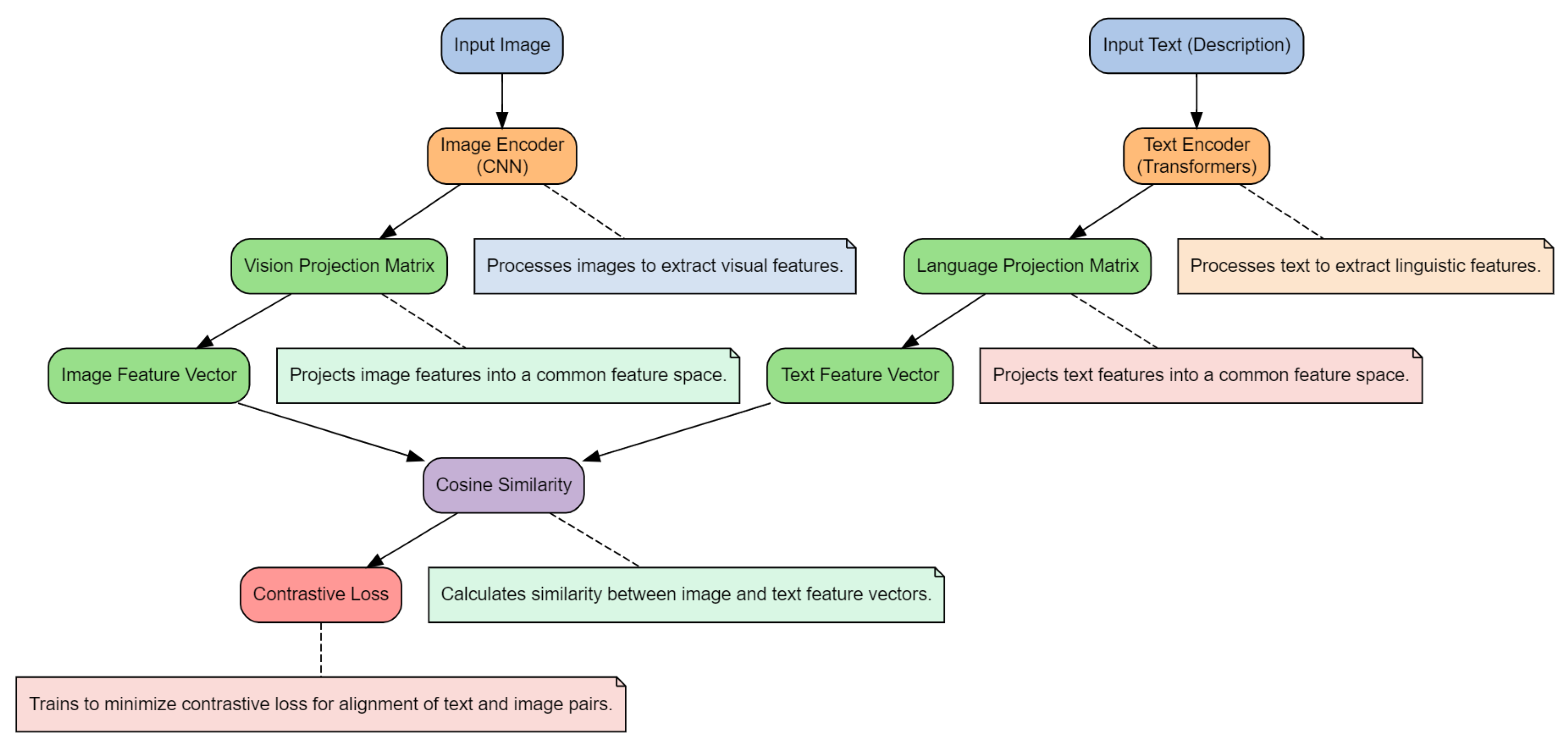
Given a text description T and the corresponding image I, DALL-E learns to maximize the likelihood of the image given the text, represented as:
where represents the i-th token of the image, and represents all preceding tokens. The transformer is trained using maximum likelihood estimation to predict each token in the sequence.
The image tokens are derived using a discrete VAE, where an image is compressed into a series of discrete latent variables. This two-stage process—first encoding the image into tokens and then generating these tokens conditioned on the text—allows DALL-E to efficiently model the high-dimensional space of images.
DALL-E showcases impressive capabilities in generating creative and contextually accurate images from prompts, such as "a two-story house shaped like a shoe" or "an astronaut riding a horse in a photorealistic style." These abilities make DALL-E useful for applications in content creation, design, education, and artistic exploration. By combining language and vision, DALL-E pushes the boundaries of what multi-modal transformers can achieve.
3.5.3. VisualBERT
VisualBERT, introduced by Li et al. in 2019[54], is a multi-modal transformer model designed to integrate vision and language for tasks requiring joint understanding of text and images. By extending the BERT architecture, VisualBERT processes both textual and visual inputs, aligning them in a shared representation space. This approach enables the model to excel in tasks such as visual question answering, image captioning, and visual reasoning.
VisualBERT adapts the BERT architecture by incorporating visual embeddings alongside textual embeddings. The input consists of: 1. Text Tokens: Processed as in BERT, each token is represented as a word embedding. 2. Image Regions: Represented using region-based feature embeddings extracted from an object detection model (e.g., Faster R-CNN). Each region’s features are projected into the same dimensional space as the text embeddings.
The model processes these embeddings jointly using transformer layers, where self-attention allows interaction between visual and textual modalities. To align the modalities, special embeddings, such as segment and positional embeddings, are added to distinguish text from visual inputs.
For an image I and corresponding text T, the input to VisualBERT is represented as:
where are word embeddings for the text tokens, and are visual embeddings for the image regions. The model computes a joint representation H using transformer layers:
The output embeddings H capture contextual relationships across both text and image, enabling cross-modal reasoning.
VisualBERT is effective in multi-modal tasks such as: - Visual Question Answering (VQA): Answering questions about an image by reasoning over both text and image features. - Image Captioning: Generating descriptive captions for images by aligning visual regions with textual descriptions. - Visual Commonsense Reasoning (VCR): Understanding implicit relationships and reasoning over visual and textual elements.
VisualBERT has demonstrated competitive performance across these tasks, highlighting its ability to unify vision and language effectively. Its architecture has inspired further research into multi-modal transformers and their applications.
3.5.4. Flamingo
Flamingo, introduced by DeepMind in 2022[17], is a multi-modal transformer designed to handle both vision and language tasks seamlessly. Flamingo excels at processing image and text sequences together, making it capable of tasks like visual question answering, caption generation, and cross-modal reasoning. One of Flamingo’s defining features is its ability to adapt to diverse tasks without task-specific fine-tuning, leveraging large-scale pretraining and in-context learning.
Flamingo combines a frozen pre-trained vision model (e.g., a convolutional neural network or vision transformer) with a language model. The visual input is first encoded into embeddings using the vision model, and these embeddings are then integrated with text embeddings in the transformer’s layers. The architecture allows bi-directional interactions between the modalities while maintaining the ability to process sequences of variable lengths.
The model incorporates: 1. Vision Encoder: Encodes image inputs into compact feature representations. 2. Language Model: Processes text and integrates visual features through cross-attention mechanisms. 3. Cross-Attention Layers: Facilitate alignment and interaction between visual and textual embeddings.
Given an image I and a sequence of text tokens , Flamingo produces a joint representation by combining the visual embeddings V and text embeddings T using cross-attention. The joint representation is computed as:
where H captures the contextualized representations of both modalities.
The model is pre-trained on a large-scale dataset of image-text pairs using objectives like contrastive learning and language modeling, enabling it to generalize across tasks with minimal adaptation.
Flamingo is versatile and effective in tasks such as: - Visual Question Answering: Generating answers based on a given image and question. - Image Captioning: Producing detailed captions for images. - Few-Shot Learning: Adapting to novel tasks with minimal examples by leveraging in-context learning.
Flamingo’s ability to unify vision and language without extensive fine-tuning makes it a significant step forward in multi-modal AI, demonstrating strong performance across diverse benchmarks Figure 4.
3.5.5. FLAVA (A Foundational Model for Language and Vision)
FLAVA, introduced by Singh et al. in 2022[55], is a multi-modal transformer designed as a foundational model for both language and vision tasks. FLAVA supports uni-modal, cross-modal, and multi-modal tasks, making it a versatile model capable of bridging the gap between textual and visual understanding. By unifying multiple modalities within a single framework, FLAVA enables coherent representations across diverse data types and tasks, such as classification, retrieval, and multi-modal reasoning.
FLAVA employs a modular architecture with three main components: 1. Text Encoder: Processes text inputs using a transformer-based language model. 2. Vision Encoder: Encodes image inputs into feature embeddings using a vision transformer (ViT). 3. Multi-Modal Encoder: Combines the outputs from the text and vision encoders, using a shared transformer to learn joint representations for vision-language tasks.
The architecture allows for independent uni-modal processing while enabling cross-modal alignment through the multi-modal encoder, making FLAVA suitable for tasks requiring varying levels of modality interaction.
FLAVA uses multiple training objectives to optimize uni-modal and multi-modal performance. These include: - Masked Language Modeling (MLM): For text inputs, a subset of tokens is masked, and the model predicts the masked tokens. - Masked Image Modeling (MIM): For visual inputs, patches of the image are masked, and the model reconstructs them. - Contrastive Loss: Aligns visual and textual representations by maximizing the similarity between matching pairs and minimizing it for non-matching pairs. - Matching Loss: Determines whether an image-text pair corresponds to each other.
Formally, given a text T and image I, the shared embedding space is learned by minimizing:
FLAVA is designed for a wide range of applications, including: - Uni-Modal Tasks: Text classification, image recognition, and object detection. - Cross-Modal Tasks: Image captioning, visual question answering, and text-to-image retrieval. - Multi-Modal Tasks: Joint reasoning over text and image pairs for complex tasks.
FLAVA serves as a robust and flexible foundational model, advancing multi-modal AI by integrating vision and language seamlessly. Its architecture and training strategy set a new standard for models capable of both uni-modal and multi-modal learning.
3.6. Generative Models
Generative models are a class of machine learning models designed to generate new data instances that resemble a given dataset. Unlike discriminative models, which focus on classifying or labeling data, generative models aim to understand the underlying data distribution and synthesize new samples from it. These models have gained significant attention for their ability to create realistic images, text, audio, and even videos.
Generative models can be implemented using various architectures, including Variational Autoencoders (VAEs), Generative Adversarial Networks (GANs), and transformer-based architectures like GPT and DALL-E. By leveraging probabilistic modeling, these architectures learn the relationships and patterns in the input data and use them to generate novel outputs.
Applications of generative models span diverse fields, including natural language processing (e.g., text generation), computer vision (e.g., image synthesis), and audio processing (e.g., speech generation). Their ability to create high-quality synthetic data has also made them invaluable in data augmentation, creative industries, and simulation-based research.
3.6.1. Autoencoders
Autoencoders, introduced by Hinton and Salakhutdinov in 2006[56], are a type of neural network designed for unsupervised learning, where the goal is to learn an efficient representation (or encoding) of input data. Autoencoders are commonly used for dimensionality reduction, feature extraction, and generative tasks. They consist of two primary components: 1. Encoder: Maps the input data to a compressed latent space representation. 2. Decoder: Reconstructs the original data from the latent representation.
The training objective of an autoencoder is to minimize the reconstruction loss, ensuring that the output closely resembles the input. This is typically achieved by optimizing the mean squared error (MSE) or binary cross-entropy (BCE) between the input x and the reconstructed output :
An autoencoder is composed of: - Input Layer: Takes the raw input data. - Hidden Layers (Encoder): Compresses the input data into a low-dimensional latent representation. - Latent Space: Encodes the compressed features, representing the essential information. - Hidden Layers (Decoder): Expands the latent representation back to the original data dimensions. - Output Layer: Produces the reconstructed version of the input.
Autoencoders are widely used in: - Dimensionality Reduction: As a non-linear alternative to Principal Component Analysis (PCA). - Anomaly Detection: Identifying deviations in data by observing reconstruction errors. - Data Denoising: Removing noise from input data by learning clean representations. - Generative Models: Serving as a foundation for advanced architectures like Variational Autoencoders (VAEs).
While standard autoencoders are effective for tasks like feature learning and reconstruction, they may struggle with generative tasks, which led to the development of extensions like VAEs. Nonetheless, autoencoders remain a fundamental building block in representation learning and generative modeling.
3.6.2. Variational Autoencoders (VAE)
Variational Autoencoders (VAE), introduced by Kingma and Welling in 2013[57], are a generative model that extends traditional autoencoders by introducing probabilistic latent variables. Unlike standard autoencoders, which compress data deterministically, VAEs model the latent space as a probability distribution, enabling the generation of new data samples by sampling from this learned distribution. This makes VAEs particularly useful for generative tasks.
The VAE architecture consists of: 1. Encoder: Maps the input x to the parameters of a latent Gaussian distribution: mean and variance . The encoder outputs these parameters, which define the latent variable z. 2. Latent Space: Samples latent variables z from the learned Gaussian distribution . 3. Decoder: Reconstructs the input x from the sampled latent variable z, modeling the conditional distribution .
The training objective of a VAE maximizes the evidence lower bound (ELBO), which balances reconstruction quality and latent space regularization:
- The first term, , ensures accurate reconstruction of the input data. - The second term, , is the Kullback-Leibler (KL) divergence, which regularizes the latent space by aligning the approximate posterior with a prior distribution , typically a standard Gaussian .
VAEs are widely used for: - Image Synthesis: Generating realistic images by sampling from the learned latent space. - Data Augmentation: Creating variations of existing data to improve model robustness. - Anomaly Detection: Identifying outliers by observing reconstruction errors or deviations in latent representations. - Representation Learning: Learning meaningful latent embeddings for downstream tasks.
VAEs bridge the gap between deterministic encoding and generative modeling, providing a principled probabilistic framework for learning latent representations and generating data. They have inspired many extensions, including Conditional VAEs and applications in diverse fields such as computer vision and bioinformatics.
3.6.3. Generative Adversarial Networks (GANs)
Generative Adversarial Networks (GANs), introduced by Goodfellow et al. in 2014[58], are a class of generative models that employ a game-theoretic approach to generate realistic data. GANs consist of two neural networks, a **Generator** and a **Discriminator**, that are trained simultaneously in a zero-sum game. The Generator creates synthetic data, while the Discriminator evaluates the authenticity of the data, distinguishing between real and generated samples. This adversarial setup drives the Generator to improve its outputs over time, producing data that closely resembles the real distribution.
1. Generator: Takes a random noise vector z sampled from a prior distribution (e.g., Gaussian or uniform) and generates synthetic data . 2. Discriminator: Processes both real and generated data, outputting a probability representing the likelihood that the input is real. The Discriminator is optimized to correctly classify real and fake samples, while the Generator aims to fool the Discriminator.
The training objective of GANs is a minimax optimization problem, defined as:
- The Discriminator D is trained to maximize the probability of correctly classifying real and fake data. - The Generator G is trained to minimize , effectively improving its ability to generate realistic samples.
This adversarial process alternates between optimizing D and G, resulting in a Generator that produces increasingly realistic outputs.
GANs are widely used in: - Image Synthesis: Creating realistic images (e.g., StyleGAN for human faces). - Data Augmentation: Generating additional training data to improve model robustness. - Image-to-Image Translation: Tasks like converting sketches to realistic images (e.g., Pix2Pix) or changing image styles (e.g., CycleGAN). - Anomaly Detection: Identifying outliers by comparing real data to generated distributions. - Creative Applications: Generating art, music, and other creative content.
While GANs are powerful, training them can be challenging due to instability and issues like mode collapse, where the Generator produces limited diversity in outputs. Despite these challenges, GANs remain a cornerstone of generative modeling, inspiring numerous variations and applications in fields such as computer vision, medicine, and entertainment.
4. Explainable AI Techniques
Explainable Artificial Intelligence (XAI) encompasses methods and techniques aimed at making the decision-making processes of AI models transparent and understandable to humans. This is particularly critical in high-stakes fields such as healthcare, finance, and law, where trust, transparency, and accountability are essential. XAI techniques can broadly be classified into several primary categories. Each category addresses different aspects of interpretability, providing tools to understand both the inner workings of models and the factors driving their predictions. Figure presents a hierarchical organization of these XAI techniques, highlighting the key methods within each category. A detailed explanation of these categories is provided below.
4.1. Model-Specific Explainability
Model-specific explainability refers to AI models whose structure inherently makes their decision-making processes transparent and interpretable. These models are designed in a way that their predictions can be easily understood without the need for additional interpretability techniques. However, while these models are simple to explain, they may lack the complexity needed to capture intricate patterns in data. Below are some key techniques under model-specific explainability.
- Decision Trees: Decision trees are inherently interpretable models that work by breaking down data into simple decision rules, leading to a final outcome. Each path from the root to a leaf represents a series of decisions, making it easy for users to follow and understand the reasoning behind a prediction. However, decision trees may overfit to training data, which can reduce their reliability on unseen data [4].
- Linear Models: Linear models are straightforward, as they quantify the relationship between input variables and the output through coefficients. The size of the coefficient indicates how much influence each variable has on the outcome. While linear models are easy to interpret, they assume linear relationships and may miss complex, nonlinear patterns [2].
Model-specific interpretability techniques are designed to leverage the unique characteristics and architectures of specific machine learning models to generate meaningful explanations. The diagram categorizes these methods across different model types. For reinforcement learning, techniques such as policy visualization and reward attribution are used to interpret state-action values and understand decision-making policies. In clustering and unsupervised models, centroid analysis and distance-based explanations provide insights into how data points are grouped, while dimensionality reduction visualization aids in understanding feature distributions. Transformers rely on attention mechanisms, such as token contribution analysis and head-wise attention, to identify relevant input components and explain sequence-based predictions. Ensemble models use feature importance aggregation and analysis of individual model contributions to understand collective decision-making. Bayesian models are explained using posterior analysis and uncertainty quantification, providing insights into parameter distributions and probabilistic reasoning. For deep neural networks, methods like saliency maps, Grad-CAM, and integrated gradients highlight the most important features or input regions responsible for predictions. Support Vector Machines (SVMs) rely on kernel visualization and decision boundary inspection for interpretability. In linear and logistic regression models, coefficient analysis and odds ratios explain feature contributions and standardized effects. Lastly, tree-based models utilize path analysis and decision rule extraction to highlight feature importance and interpret predictive pathways. Each of these techniques is specifically adapted to the model type, offering detailed and accurate explanations (refer to Figure 5).
Table 5 provides a comparison of Decision Trees and Linear Models regarding their interpretability and performance.
4.2. Model-Agnostic Methods
Model-agnostic methods offer interpretability solutions that can be applied to any machine learning model, regardless of its complexity. These techniques do not depend on the internal workings of the model but instead focus on explaining the outputs of the model after training. Model-agnostic methods are versatile, but they can sometimes struggle to provide insights into the global behavior of the model. Below, we summarize the most commonly used model-agnostic methods.
- LIME (Local Interpretable Model-Agnostic Explanations): LIME explains individual predictions by building a simpler, interpretable model around a specific prediction. This method works with any machine learning model and helps users understand the factors that contributed to a particular decision. However, LIME only provides local explanations, which may not generalize to the model’s overall behavior [59].
- SHAP (SHapley Additive Explanations): SHAP uses game theory to distribute the contribution of each feature fairly in a prediction. It offers consistent and clear explanations but can be computationally intensive, especially for large datasets or complex models [60].
- Partial Dependence Plots (PDP): PDPs illustrate the relationship between a feature and the predicted outcome, helping users understand whether a feature has a linear or nonlinear effect on the outcome. However, PDPs may provide misleading interpretations if features are highly correlated [29].
- Individual Conditional Expectation (ICE) Plots: ICE plots are similar to PDPs but focus on individual predictions, showing how changes in a feature affect each data point’s prediction. ICE plots offer more detailed insights but can become difficult to interpret with large datasets [61].
- Feature Importance: This method assigns a score to each feature based on its contribution to the model’s prediction accuracy. Feature importance helps identify which features are most influential, but the results can vary if the features are interdependent [28].
- Surrogate Models: Surrogate models create simplified approximations of complex systems, making predictions more interpretable. However, while surrogate models reduce computational costs, they may not capture the full complexity of the original model [62].
Model-agnostic interpretability techniques offer a flexible and universal approach to explaining predictions from machine learning models. These techniques do not rely on the internal workings of the model, making them applicable to any machine learning algorithm. The diagram highlights six prominent methods used in this context. Surrogate models involve training simple, interpretable models, such as decision trees, to approximate complex black-box models and generate insights. Feature importance techniques evaluate and rank features based on their contribution to the model’s predictions, providing a global understanding of the model’s behavior. Individual Conditional Expectation (ICE) plots visualize the effect of varying a feature’s values on predictions for individual data instances, helping to understand localized effects. Partial Dependence Plots (PDP), on the other hand, show the average impact of a feature by varying its values and plotting the resulting partial dependencies, providing global insights. SHAP (SHapley Additive exPlanations) computes feature contributions based on Shapley values to explain predictions both globally and locally. Finally, LIME (Local Interpretable Model-agnostic Explanations) generates perturbed samples around individual predictions and trains a simple model locally to explain specific outcomes. These techniques ensure interpretability in diverse machine learning applications while remaining independent of the underlying model structure (see Figure 6).
Table 6 presents a comparison of various machine learning interpretability techniques.
4.3. Post-Hoc Explainability
Post-hoc explainability methods focus on providing explanations for models after predictions have been made. These techniques are particularly useful for black-box models, such as deep neural networks, where understanding the inner workings is difficult. Post-hoc techniques make these complex models more interpretable without affecting their prediction performance. Below are some of the most prominent post-hoc explainability methods.
- Counterfactual Explanations: Counterfactual explanations describe how changes to certain inputs would have led to different outcomes. For example, in credit applications, a counterfactual explanation could indicate that a loan would have been approved if the applicant had a higher income. Generating realistic counterfactuals can be challenging, but they provide actionable insights for users [63].
- Saliency Maps: Saliency maps are typically used in image-based models to highlight which parts of an image were most important for the model’s decision. Although they provide a visual explanation, saliency maps can be inconsistent across different models and datasets [64].
- Attention Mechanisms: Attention mechanisms, often used in neural networks, focus on the most relevant parts of the input, improving both model performance and interpretability. However, using attention mechanisms may increase the computational complexity of the model [65].
- Layer-wise Relevance Propagation (LRP): LRP explains predictions by tracing them back through the layers of a neural network, identifying which input features contributed most to the output. While LRP offers detailed insights, it can be time-consuming and difficult to apply to very deep networks [66].
- Gradient-Based Methods (e.g., Grad-CAM): These methods use gradients to identify which parts of an image influenced the model’s prediction. Gradient-based methods are commonly used in deep learning applications but may overlook finer details in the data [67].
- Explainable Boosting Machines (EBM): EBMs are an interpretable machine learning technique that combines boosting with transparency, making them both accurate and understandable. However, as the number of features increases, EBMs can become more complex [68].
Post-hoc explainability techniques are employed after model training to provide detailed explanations of model predictions and behavior. These methods allow users to analyze the decisions of complex models and extract interpretable insights. The diagram showcases several widely used post-hoc methods. Gradient-based techniques, such as Grad-CAM, compute gradients, map them to input features, and highlight the most influential features to provide explanations. Local surrogate models, such as LIME, create perturbed samples and train simple interpretable models locally to explain individual predictions. Global surrogate models, by contrast, approximate the overall behavior of the black-box model using interpretable models like decision trees. Individual Conditional Expectation (ICE) plots focus on the impact of varying a single feature on predictions for specific data instances, while Partial Dependence Plots (PDP) provide the average effect of feature variations on predictions across the dataset. Attention mechanisms identify attention scores and generate heatmaps to highlight relevant inputs, making them particularly useful in natural language processing and computer vision tasks. Saliency maps compute gradients for input data, such as images, to identify and visualize salient regions. Counterfactual explanations involve generating alternative inputs and comparing them to original inputs to determine the minimal changes required for a different prediction, enabling actionable insights. Finally, feature attribution methods, such as SHAP and LIME, compute feature contributions and importance scores to provide both global and local explanations. These techniques enhance understanding of complex models, ensuring transparency and trust (see Figure 7).
Table 7 presents a comparison of machine learning interpretability techniques.
4.4. Perspectives in Explainability
Explainability techniques in machine learning can be classified based on different perspectives. These include global vs. local explainability and intrinsic vs. post-hoc interpretability. The following subsections explore these perspectives and their implications for machine learning models.
- Global vs. Local Explanations: Global explanations aim to provide insights into how a model behaves across all data points, while local explanations focus on explaining individual predictions. Both approaches offer valuable perspectives, depending on whether the goal is to understand the overall behavior of the model or specific decisions. Table 8 provides a comparison of global and local interpretability approaches in machine learning models.
Table 8.
Comparison of Global and Local Interpretability Approaches in Machine Learning Models
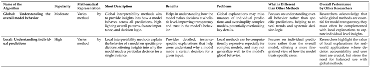 |
- Intrinsic vs. Post-Hoc: Intrinsic interpretability refers to models that are naturally transparent, such as decision trees and linear models. Post-hoc interpretability involves explaining black-box models after predictions have been made, using techniques like LIME or SHAP. Table 9 presents a comparison of intrinsic and post-hoc interpretability methods.
Table 9.
Comparison of Intrinsic and Post-hoc Interpretability Methods
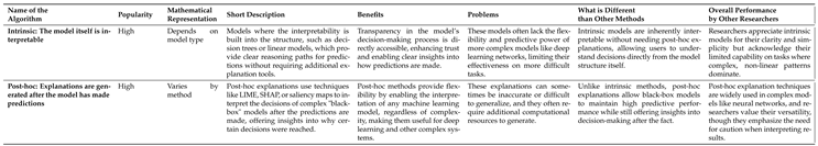 |
- Human Interpretability: Human interpretability measures how easily a human can understand the explanations provided by a model. This is critical for ensuring trust and usability in AI systems. Table 10 presents an evaluation of model interpretability based on human understanding of the explanations.
Table 10.
Evaluation of Model Interpretability: Human Understanding of Explanations
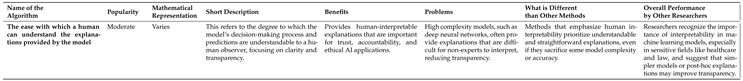 |
Explainable AI techniques are essential for building trust and ensuring that AI models are transparent and interpretable. Some models, like decision trees and linear models, are naturally interpretable, while others, like neural networks, require additional explainability techniques such as LIME, SHAP, and counterfactual explanations. A balance must be struck between explainability and accuracy, and ongoing research is addressing these challenges to ensure that AI models are both performant and understandable for real-world applications.
5. Explainable AI in Robotics
Explainable AI in robotics has emerged as an important field as robots increasingly take on complex roles in various domains such as healthcare, manufacturing, and autonomous systems [69,70]. This field focuses on the development of artificial intelligence (AI) systems capable of providing clear, interpretable explanations for their decisions and actions. Explainability is crucial for enhancing trust, transparency, and effective human-robot interaction, particularly in sectors where safety, accountability, and ethical considerations are paramount [71]. The ability for both developers and end-users to understand why a robot made a particular decision, how it processed information, and what factors influenced its behavior is essential. It ensures effective debugging, promotes safety, and facilitates the alignment of robotic systems with ethical standards [72]. Figure 8 illustrates the hierarchical structure of Explainable AI in Robotics, which is organized into key categories, each addressing different aspects of explainability. A detailed explanation of these categories is provided below.
5.1. Explainable Robotics for Human-Robot Interaction
Explainability in human-robot interaction is essential for improving communication and cooperation between robots and humans. By providing interpretable explanations for actions and decisions, robots can better align with human expectations and foster trust in collaborative environments[71]. Table 11 presents a comparison of various methods for explainability in human-robot interaction.
- Saliency Maps: Saliency maps visually highlight the regions of an image that most significantly influence the robot’s decision-making process. This technique provides a visual explanation for deep learning models and is useful for tasks such as image recognition. However, saliency maps can sometimes produce noisy results and may be difficult to interpret reliably [64].
- Attention Mechanisms: Attention mechanisms allow the robot to focus on the most relevant parts of input data by assigning different levels of importance to different features. This approach enhances both performance and interpretability, especially in tasks such as machine translation and image captioning [65].
- Natural Language Explanations: Natural language explanations enable robots to articulate their decision-making processes in plain, everyday language, bridging the gap between complex AI decisions and human understanding. This makes AI systems more accessible and transparent to non-expert users [73].
5.2. Transparency in Autonomous Robots
As autonomous robots increasingly operate in complex environments, ensuring transparency in their decision-making processes becomes critical for user trust and safety [74]. Transparency methods help users understand how robots make decisions and what factors influence these decisions. Table 12 provides a comparison of techniques for enhancing transparency in autonomous robotic systems.
- LIME: Local Interpretable Model-agnostic Explanations (LIME) generates locally interpretable models around specific predictions, allowing users to understand why a particular decision was made by a robot. While LIME is useful for building trust, it may not capture the full complexity of the global model [59].
- SHAP: SHapley Additive exPlanations (SHAP) use game theory to attribute the contribution of each feature to a robot’s decision. SHAP provides consistent and clear explanations but can be computationally expensive for complex models [60].
- Rule-Based Explanations: Rule-based explanations offer straightforward decision paths using IF-THEN rules. While these are easy to understand, they may be too rigid to capture the nuances present in more complex AI models [75].
Table 12.
Comparison of Popular Machine Learning Explanation Methods
| Name of Algorithm | Popularity | Description | Benefits | Challenges |
|---|---|---|---|---|
| LIME | High | LIME explains machine learning predictions by creating a simple model around specific predictions. |
Helps users understand why a model made a particular prediction, which builds trust in complex models. |
May miss some of the complex factors in the original model. |
| SHAP | High | SHAP assigns importance scores to each feature of a prediction using game theory. |
Provides consistent explanations for how features impact predictions, using a sound mathematical framework. |
Can be slow and resource-heavy for complex models. |
| Rule-based Explanations | Low | Uses IF-THEN rules to explain decisions step-by-step. |
Easy to understand, showing clearly how decisions are made. |
Too rigid for complex AI, may miss important nuances. |
5.3. Interpretable Learning for Robotic Control
Interpretable learning is fundamental for robotic control, especially in scenarios where the robot must learn and adapt autonomously. Interpretability ensures that the robot’s learning process can be understood and fine-tuned by developers and users alike[76]. Table 13 compares various methods of interpretable learning for robotic control.
- Policy Summaries: Policy summaries focus on learning the underlying reward function from a robot’s behavior. This is particularly useful in cases where specifying explicit rewards is challenging, though it can be difficult to infer the true objective from limited demonstrations [77].
- Visualizing Learned Behaviors: Visualizing learned behaviors helps to understand the robot’s actions during reinforcement learning. Although this technique aids in interpreting learning outcomes, it can be challenging to implement in complex environments [78].
- Hierarchical Reinforcement Learning (HRL): HRL breaks complex tasks into smaller subtasks, enabling robots to learn efficiently. However, poorly structured subtasks can hinder learning efficiency and overall performance [79].
Table 13.
Comparison of Reinforcement Learning Methods
| Name of Algorithm | Popularity | Description | Benefits | Challenges |
|---|---|---|---|---|
| Policy Summaries (Inverse Reinforcement Learning) | High | Focuses on learning the reward function from an agent’s behavior instead of knowing it beforehand, like in standard reinforcement learning. |
Allows us to learn from demonstrations without needing an explicit reward function, useful for tasks where it is difficult to define the reward in advance. |
It can be hard to figure out the true reward from limited demonstrations, as different rewards can lead to the same behavior. |
| Visualizing Learned Behaviors (Deep Q-networks) | High | A deep learning-based reinforcement learning algorithm that learns optimal actions by interacting with the environment. |
Can learn directly from high-dimensional input, such as images from video games, without needing pre-defined features. |
Difficult to train, especially in complex environments or when rewards are sparse, leading to unstable results. |
| Hierarchical Reinforcement Learning (HRL) | Moderate | Divides complex tasks into smaller, manageable subtasks, improving learning efficiency. |
By breaking down the task, HRL agents can learn faster and achieve better results compared to standard RL approaches. |
Poorly designed subtasks can lead to suboptimal learning, limiting the agent’s overall performance. |
5.4. Explainable AI in Collaborative Robotics
Achieving effective collaboration between humans and robots necessitates a high degree of explainability to ensure the predictability and transparency of robotic actions. Explainable AI in collaborative robotics focuses on developing intelligent systems that can work seamlessly alongside humans by providing clear and comprehensive insights into their decision-making processes [71]. This allows both developers and end-users to better understand the reasoning and factors underlying the robots’ actions, which is crucial for fostering trust, improving safety, and aligning the systems with ethical standards. Table 14 provides a comparative analysis of the various methods employed to enhance explainability in collaborative robotics.
- Predictive Explanations: These models provide transparent decision-making processes, which can help users understand predictions, although simpler models may sometimes sacrifice accuracy [80].
- User Feedback Integration: User feedback integration enables robots to refine their behaviors through active user input, ensuring models are aligned with real-world needs. Designing intuitive and efficient feedback systems is crucial for success [81].
- Context-Aware Explanations: Context-aware explanations tailor responses based on the user’s current task or situation, improving relevance and trust. However, accurately identifying the relevant context can be challenging [59].
Table 14.
Comparison of Machine Learning Explanation Methods
| Name of Algorithm | Popularity | Description | Benefits | Challenges |
|---|---|---|---|---|
| Predictive Explanations (Interpretable Machine Learning) | Moderate | Builds models that are easy for humans to understand. The structure and decision-making process are clear and transparent. |
Allows people to see why a model made a certain prediction, building trust, especially in fields like healthcare or finance. |
Simple models may not be as accurate as complex models, especially for tasks that require finding complex patterns. |
| User Feedback Integration | High | Focuses on getting human feedback to improve machine learning models. Humans actively participate in refining models to make them more useful. |
Leads to models that are more user- friendly and aligned with real-world needs by incorporating human expertise. |
Designing easy ways for humans to give feedback without overwhelming them is crucial for success. |
| Context-Aware Explanations | Low | Provides explanations that are tailored to the user’s specific situation or task, considering their background and needs. |
Users find the explanations more relevant and easier to understand, which builds trust in the AI system. |
It can be challenging to identify the right context and adjust explanations effectively. |
5.5. Explainable AI for Safety in Robotics
Ensuring safety in robotics is paramount, especially in high-stakes environments like healthcare or autonomous driving. Explainable AI methods focused on safety help identify potential risks and provide understandable reasoning for a robot’s actions to avoid dangerous outcomes [82]. These methods can also inform the design and development of more robust and trustworthy robotic systems. Table 15 presents a comparison of various explainable AI techniques that can be applied to ensure safety in robotics, including their strengths, limitations, and potential applications.
- Anomaly Detection: Anomaly detection identifies unusual patterns in robot behavior, aiding in the detection of system failures or operational anomalies. However, balancing the detection of true anomalies while minimizing false alarms can be difficult [83].
- Counterfactual Explanations: These explanations illustrate how changing specific conditions could have altered the robot’s actions. While helpful for understanding potential future adjustments, generating realistic counterfactuals can be complex [63].
- Risk Assessment Models: Risk assessment models identify potential harms associated with AI systems. Although useful for promoting safety, they do not inherently guarantee bias-free operation [84].
Table 15.
Comparison of Machine Learning and Explainable AI Methods
| Name of Algorithm | Popularity | Description | Benefits | Challenges |
|---|---|---|---|---|
| Anomaly Detection | High | Detects unusual patterns in data that differ from normal behavior, often used for identifying system failures, fraud, or other critical events. |
Can detect unknown threats or issues without prior knowledge, making it useful for identifying new forms of attacks or unexpected situations. |
Balancing accurate detection of anomalies with minimizing false alarms is challenging. |
| Counterfactual Explanations | High | Explains decisions by showing how outcomes could change if specific conditions were different, like how a higher income could lead to loan approval. |
Helps users understand how to change future outcomes, without needing detailed technical knowledge of the decision process. |
Ensuring these explanations are realistic and achievable in the real world can be difficult. |
| Risk Assessment Models | High | Identify potential harms in AI systems, helping to manage risks from design to deployment. |
Ensures AI is accurate, trustworthy, and transparent by assessing risks related to explainability, which helps build user trust. |
Overreliance on explanations may lead to a false sense of safety or fairness, even though explanations alone don’t guarantee bias-free AI systems. |
5.6. Explainable AI for Adaptive Robotics
Adaptive robotics requires the ability to adjust to dynamic environments in real-time. Explainable AI in adaptive robotics ensures that the robot’s adjustments are transparent and understandable to human operators, making it easier to correct or guide the robot’s behavior when necessary. Table 16 compares methods for Explainable AI in adaptive robotics.
- Interactive Learning: Interactive learning allows robots to acquire new information through interactions with their environment, enhancing learning efficiency. However, designing effective strategies for interaction remains a challenge [85].
- User-Guided Adjustments: User-guided adjustments permit users to modify the robot’s behavior based on their expertise, improving model accuracy. However, user biases may affect fairness and generalization [81].
- Adaptive Models with Feedback Loops: These models adjust dynamically based on real-time data, improving performance in dynamic environments. However, they are sensitive to noisy feedback, which can degrade overall performance [86].
Table 16.
Comparison of Interactive and Adaptive Learning Methods
| Name of Algorithm | Popularity | Description | Benefits | Challenges |
|---|---|---|---|---|
| Interactive Learning (Lifelong Learning) | Moderate | Algorithms that actively learn by interacting with their environment or users, unlike traditional methods where data is passively received. |
Increases learning efficiency by allowing the algorithm to ask for needed data, making it more adaptable. |
Designing effective interaction strategies is complex. |
| User-Guided Adjustments | Moderate to High | Users can adjust or refine a model’s behavior through an interface, adding expertise to improve results. |
Lets users improve the model, making it more accurate and trustworthy, especially when data is biased. |
User bias can affect fairness if adjustments are poorly designed. |
| Adaptive Models with Feedback Loops | Moderate | Models adjust settings based on real-time feedback, used in dynamic environments like finance or autonomous vehicles. |
Constant learning from real-time data improves accuracy and performance in changing environments. |
Sensitive to noisy feedback, which may reduce performance. |
5.7. Ethical and Trustworthy Robotics through Explainable AI
The implementation of ethical standards and trustworthy behavior in robots is a growing concern as AI systems become more integrated into society. Explainable AI ensures that robots comply with ethical guidelines and can be held accountable for their actions. Explainable AI techniques, such as interpretable machine learning models and transparency in decision-making processes, can help build trust and understanding between humans and robots [87]. This is crucial as robots take on increasingly complex roles in sectors like healthcare, manufacturing, and autonomous systems. Table 17 compares various methods for promoting ethical and trustworthy robotics through the use of explainable AI.
- Ethical Rule Enforcement: This approach ensures that robots adhere to ethical guidelines, reducing bias and promoting fairness. However, defining universal ethical rules can be subjective and context-dependent [88].
- Explainable Decision-Making Frameworks: These frameworks provide transparency in decision-making, building user trust. Balancing the simplicity of explanations with model accuracy can be challenging [89].
- Compliance Auditing: Compliance auditing ensures that robots comply with regulatory and ethical standards, minimizing risk and enhancing operational credibility. Keeping up with changing regulations presents a challenge [90].
Table 17.
Comparison of Ethical and Explainable AI Methods
| Name of Algorithm | Popularity | Description | Benefits | Challenges |
|---|---|---|---|---|
| Ethical Rule Enforcement | Moderate | Implements rules to make sure AI systems follow ethical standards. |
Reduces harm, bias, and promotes fairness and accountability. |
Hard to define universal ethics, as rules can be subjective. |
| Explainable Decision-Making | High | Makes AI decisions clear and understandable to users. |
Builds trust by explaining how decisions are made. |
Difficult to balance simplicity with accuracy in complex models. |
| Compliance Auditing | High | Checks if organizations follow laws and internal policies. |
Reduces risks, improves efficiency, and enhances credibility. |
Keeping up with changing laws is a challenge. |
6. Conclusion
This review has explored the intersection of machine learning, deep learning, large language models, multimodal models, and explainable AI in the context of robotics, highlighting their transformative potential. By categorizing key AI methodologies, including supervised, unsupervised, and reinforcement learning, and examining advanced architectures such as convolutional neural networks and transformers, we emphasized their applications and capabilities. Special attention was given to explainable AI, showcasing its critical role in fostering transparency, trust, and ethical integration, particularly in robotics for human-robot collaboration, autonomous decision-making, and safety-critical applications. Additionally, the integration of multimodal models has expanded robotic capabilities, enabling seamless interaction between different data modalities. As AI continues to evolve, future research must focus on enhancing explainability, adaptability, and ethical considerations to ensure that intelligent systems remain transparent, reliable, and aligned with human values, ultimately driving trustworthy advancements in robotics.
Acknowledgments
This research is a collaborative effort between the Islamic University of Madinah and Prince Sultan University. We extend our gratitude to both institutions for their support in facilitating this study. Additionally, we acknowledge Prince Sultan University for generously covering the article processing charges for this publication.
Conflicts of Interest
Declare conflicts of interest or state “The authors declare no conflicts of interest.” Authors must identify and declare any personal circumstances or interest that may be perceived as inappropriately influencing the representation or interpretation of reported research results. Any role of the funders in the design of the study; in the collection, analyses or interpretation of data; in the writing of the manuscript; or in the decision to publish the results must be declared in this section. If there is no role, please state “The funders had no role in the design of the study; in the collection, analyses, or interpretation of data; in the writing of the manuscript; or in the decision to publish the results”.
References
- Artificial Intelligence Market Size, Share & Trends Analysis Report By Solution, By Technology, By End Use, By Region, And Segment Forecasts, 2022 - 2030. Grand View Research 2022.
- Friedman, J.; Hastie, T.; Tibshirani, R. The Elements of Statistical Learning: Data Mining, Inference, and Prediction; Springer, 2001.
- Bishop, C.M. Pattern Recognition and Machine Learning; Springer, 2006.
- Quinlan, J.R. Induction of Decision Trees. Machine Learning 1986, 1, 81–106.
- Lloyd, S.P. Least Squares Quantization in PCM. IEEE Transactions on Information Theory 1982, 28, 129–137.
- Jolliffe, I.T. Principal Component Analysis; Springer, 2002.
- Watkins, C.J.; Dayan, P. Q-Learning. Machine Learning 1992, 8, 279–292.
- Mnih, V.; Kavukcuoglu, K.; Silver, D.; Rusu, A.A.; Veness, J.; Bellemare, M.G.; Graves, A.; Riedmiller, M.; Fidjeland, A.K.; Ostrovski, G. Human-level control through deep reinforcement learning. Nature 2015, 518, 529–533. [CrossRef]
- LeCun, Y.; Bottou, L.; Bengio, Y.; et al. Gradient-Based Learning Applied to Document Recognition. Proceedings of the IEEE 1998, 86, 2278–2324. [CrossRef]
- Elman, J.L. Finding structure in time. Cognitive Science 1990, 14, 179–211.
- Krizhevsky, A.; Sutskever, I.; Hinton, G.E. Imagenet classification with deep convolutional neural networks. Advances in Neural Information Processing Systems 2012, pp. 1097–1105.
- He, K.; Zhang, X.; Ren, S.; Sun, J. Deep Residual Learning for Image Recognition 2016. pp. 770–778.
- Vaswani, A.; Shazeer, N.; Parmar, N.; et al. Attention Is All You Need 2017. pp. 5998–6008.
- Ribeiro, M.T.; Singh, S.; Guestrin, C. "Why Should I Trust You?" Explaining the Predictions of Any Classifier 2016. pp. 1135–1144.
- Lundberg, S.M.; Lee, S.I. A Unified Approach to Interpreting Model Predictions 2017. pp. 4765–4774.
- Radford, A.; Kim, J.W.; Hallacy, C.; et al. Learning Transferable Visual Models From Natural Language Supervision 2021.
- Alayrac, J.B.; Donahue, J.; Luc, P.; et al. Flamingo: A Visual Language Model for Few-Shot Learning. arXiv preprint arXiv:2204.14198 2022.
- Cortes, C.; Vapnik, V. Support-vector networks. Machine Learning 1995, 20, 273–297.
- Cover, T.; Hart, P. Nearest neighbor pattern classification. IEEE Transactions on Information Theory 1967, 13, 21–27.
- Rish, I. An empirical study of the naive Bayes classifier. In Proceedings of the IJCAI 2001 Workshop on Empirical Methods in AI, 2001, Vol. 3, pp. 41–46.
- Hoerl, A.E.; Kennard, R.W. Ridge regression: Biased estimation for nonorthogonal problems. Technometrics 1970, 12, 55–67.
- Tibshirani, R. Regression shrinkage and selection via the lasso. Journal of the Royal Statistical Society: Series B (Methodological) 1996, 58, 267–288.
- Zou, H.; Hastie, T. Regularization and variable selection via the elastic net. Journal of the Royal Statistical Society: Series B (Statistical Methodology) 2005, 67, 301–320.
- Fisher, R.A. The use of multiple measurements in taxonomic problems. Annals of Eugenics 1936, 7, 179–188. [CrossRef]
- Duda, R.O.; Hart, P.E.; Stork, D.G. Pattern Classification; Wiley-Interscience, 2001.
- Pearl, J. Probabilistic Reasoning in Intelligent Systems: Networks of Plausible Inference; Morgan Kaufmann, 1988.
- Suykens, J.A.; Vandewalle, J. Least squares support vector machine classifiers. Neural Processing Letters 1999, 9, 293–300. [CrossRef]
- Breiman, L. Random forests. Machine Learning 2001, 45, 5–32.
- Friedman, J.H. Greedy function approximation: A gradient boosting machine. Annals of Statistics 2001, pp. 1189–1232. [CrossRef]
- Chen, T.; Guestrin, C. XGBoost: A scalable tree boosting system. In Proceedings of the Proceedings of the 22nd ACM SIGKDD International Conference on Knowledge Discovery and Data Mining. ACM, 2016, pp. 785–794.
- Ke, G.; Meng, Q.; Finley, T.; Wang, T.; Chen, W.; Ma, W.; Ye, Q.; Liu, T.Y. LightGBM: A highly efficient gradient boosting decision tree. In Proceedings of the Proceedings of the 31st International Conference on Neural Information Processing Systems, 2017, pp. 3149–3157.
- Dorogush, A.; Ershov, V.; Gulin, A. CatBoost: Gradient boosting with categorical features support. In Proceedings of the Proceedings of the 32nd International Conference on Neural Information Processing Systems, 2018, pp. 6638–6648.
- Freund, Y.; Schapire, R.E. A decision-theoretic generalization of on-line learning and an application to boosting. Journal of Computer and System Sciences 1997, 55, 119–139.
- Breiman, L. Bagging predictors. Machine Learning 1996, 24, 123–140.
- Wolpert, D.H. Stacked generalization. In Proceedings of the Neural Networks. Elsevier, 1992, Vol. 5, pp. 241–259.
- Kuncheva, L.I. Combining Pattern Classifiers: Methods and Algorithms; Wiley-Interscience, 2004.
- Johnson, S.C. Hierarchical clustering schemes. Psychometrika 1967, 32, 241–254. [CrossRef]
- Hyvärinen, A.; Oja, E. Independent component analysis: Algorithms and applications. Neural Networks 2000, 13, 411–430. [CrossRef]
- Reynolds, D.A. Gaussian Mixture Models. In Proceedings of the Encyclopedia of Biometrics. Springer, 2009, pp. 659–663.
- Kohonen, T. The self-organizing map. Proceedings of the IEEE 1990, 78, 1464–1480.
- Sutton, R.S.; McAllester, D.A.; Singh, S.P.; Mansour, Y. Policy gradient methods for reinforcement learning with function approximation. Advances in Neural Information Processing Systems 2000, pp. 1057–1063.
- Rumelhart, D.E.; Hinton, G.E.; Williams, R.J. Learning representations by back-propagating errors. Nature 1986, 323, 533–536. [CrossRef]
- Simonyan, K.; Zisserman, A. Very deep convolutional networks for large-scale image recognition. arXiv preprint arXiv:1409.1556 2014.
- Szegedy, C.; Liu, W.; Jia, Y.; Sermanet, P.; Reed, S.; Anguelov, D.; Erhan, D.; Vanhoucke, V.; Rabinovich, A. Going deeper with convolutions. In Proceedings of the Proceedings of the IEEE Conference on Computer Vision and Pattern Recognition, 2015, pp. 1–9.
- Huang, G.; Liu, Z.; Van Der Maaten, L.; Weinberger, K.Q. Densely connected convolutional networks. Proceedings of the IEEE Conference on Computer Vision and Pattern Recognition 2017, pp. 4700–4708.
- Hochreiter, S.; Schmidhuber, J. Long short-term memory. Neural Computation 1997, 9, 1735–1780.
- Cho, K.; Van Merrienboer, B.; Gulcehre, C.; Bahdanau, D.; Bougares, F.; Schwenk, H.; Bengio, Y. Learning phrase representations using RNN encoder-decoder for statistical machine translation. In Proceedings of the Proceedings of the 2014 Conference on Empirical Methods in Natural Language Processing (EMNLP), 2014, pp. 1724–1734.
- Devlin, J.; Chang, M.W.; Lee, K.; Toutanova, K. BERT: Pre-training of deep bidirectional transformers for language understanding. In Proceedings of the Proceedings of the 2019 Conference of the North American Chapter of the Association for Computational Linguistics: Human Language Technologies, Volume 1 (Long and Short Papers), 2019, pp. 4171–4186.
- Radford, A.; Narasimhan, K.; Salimans, T.; Sutskever, I. Improving language understanding by generative pre-training. OpenAI Blog 2018, 1, 1–12.
- Raffel, C.; Shazeer, N.; Roberts, A.; Lee, K.; Narang, S.; Matena, M.; Zhou, Y.; Li, W.; Liu, P.J. Exploring the limits of transfer learning with a unified text-to-text transformer. In Proceedings of the Proceedings of the 37th International Conference on Machine Learning, 2020, pp. 3376–3387.
- Yang, Z.; Dai, Z.; Yang, Y.; Carbonell, J.; Salakhutdinov, R.; Le, Q.V. XLNet: Generalized autoregressive pretraining for language understanding. In Proceedings of the Advances in Neural Information Processing Systems, 2019, pp. 5753–5763.
- Chowdhery, A.; Narang, S.; Devlin, J.; Bosma, M.; Mishra, G.; Roberts, A.; Barham, P.; Chung, H.W.; Sutton, C.; Gehrmann, S.; et al. Palm: Scaling language modeling with pathways. Journal of Machine Learning Research 2023, 24, 1–113.
- Ramesh, A.; Pavlov, M.; Goh, G.; Gray, S.; Voss, C.; Radford, A.; Chen, M.; Sutskever, I. Zero-shot text-to-image generation. arXiv preprint arXiv:2102.12092 2021.
- Li, L.H.; Luo, H.; Shuster, K.; Piramuthu, R.; Ueffing, N.; Berg, A.C.; Baldridge, J. VisualBERT: A simple and performant baseline for vision and language. In Proceedings of the Proceedings of the 58th Annual Meeting of the Association for Computational Linguistics, 2019, pp. 4189–4202.
- Singh, A.; Hu, R.; Adcock, A.; Batra, D.; Parikh, D.; Lee, S.; Berg, T.L.; Baldridge, J. FLAVA: A foundational language and vision alignment model. In Proceedings of the Proceedings of the 39th International Conference on Machine Learning, 2022, pp. 16734–16751.
- Hinton, G.E.; Salakhutdinov, R.R. Reducing the dimensionality of data with neural networks. Science 2006, 313, 504–507. [CrossRef]
- Kingma, D.P.; Welling, M. Auto-encoding variational Bayes. In Proceedings of the Proceedings of the 2nd International Conference on Learning Representations (ICLR), 2014.
- Goodfellow, I.; Pouget-Abadie, J.; Mirza, M.; Xu, B.; Warde-Farley, D.; Ozair, S.; Courville, A.; Bengio, Y. Generative adversarial nets. In Proceedings of the Advances in Neural Information Processing Systems, 2014, pp. 2672–2680.
- Ribeiro, M.T.; Singh, S.; Guestrin, C. "Why should I trust you?": Explaining the predictions of any classifier. In Proceedings of the Proceedings of the 22nd ACM SIGKDD International Conference on Knowledge Discovery and Data Mining. ACM, 2016, pp. 1135–1144.
- Lundberg, S.M.; Lee, S.I. A unified approach to interpreting model predictions. Advances in Neural Information Processing Systems 2017, 30.
- Goldstein, A.; Kapelner, A.; Bleich, J.; Pitkin, E. Peeking inside the black box: Visualizing statistical learning with plots of individual conditional expectation. Journal of Computational and Graphical Statistics 2015, 24, 44–65. [CrossRef]
- Craven, M.W.; Shavlik, J.W. Extracting tree-structured representations of trained networks. Advances in Neural Information Processing Systems 1996, pp. 24–30.
- Wachter, S.; Mittelstadt, B.; Russell, C. Counterfactual explanations without opening the black box: Automated decisions and the GDPR. Harvard Journal of Law & Technology 2018, 31, 841–887.
- Simonyan, K.; Vedaldi, A.; Zisserman, A. Deep inside convolutional networks: Visualising image classification models and saliency maps. arXiv preprint arXiv:1312.6034 2013.
- Bahdanau, D.; Cho, K.; Bengio, Y. Neural machine translation by jointly learning to align and translate. In Proceedings of the Proceedings of the 3rd International Conference on Learning Representations (ICLR), 2015.
- Bach, S.; Binder, A.; Montavon, G.; Klauschen, F.; Müller, K.R.; Samek, W. Pixel-wise explanations for non-linear classifier decisions by layer-wise relevance propagation. PloS one 2015, 10, e0130140. [CrossRef]
- Selvaraju, R.R.; Cogswell, M.; Das, A.; Vedantam, R.; Parikh, D.; Batra, D. Grad-CAM: Visual explanations from deep networks via gradient-based localization. In Proceedings of the Proceedings of the IEEE International Conference on Computer Vision, 2017, pp. 618–626.
- Caruana, R.; Lou, Y.; Gehrke, J.; Koch, P.; Sturm, M.; Elhadad, N. Intelligible models for healthcare: Predicting pneumonia risk and hospital 30-day readmission. In Proceedings of the Proceedings of the 21th ACM SIGKDD International Conference on Knowledge Discovery and Data Mining, 2015, pp. 1721–1730.
- Sanneman, L.; Shah, J.A. Trust considerations for explainable robots: A human factors perspective. arXiv preprint arXiv:2005.05940 2020.
- Liao, Q.V.; Sundar, S.S. Designing for responsible trust in AI systems: A communication perspective. In Proceedings of the Proceedings of the 2022 ACM Conference on Fairness, Accountability, and Transparency, 2022, pp. 1257–1268.
- De Graaf, M.M.; Dragan, A.; Malle, B.F.; Ziemke, T. Introduction to the special issue on explainable robotic systems, 2021. [CrossRef]
- Huang, S.H.; Bhatia, K.; Abbeel, P.; Dragan, A.D. Establishing appropriate trust via critical states. In Proceedings of the 2018 IEEE/RSJ international conference on intelligent robots and systems (IROS). IEEE, 2018, pp. 3929–3936.
- Ehsan, U.; Harrison, B.; Chan, L.; Riedl, M.O. Rationalization: A neural machine translation approach to generating natural language explanations. In Proceedings of the Proceedings of the 2018 AAAI Conference on Artificial Intelligence, 2018, pp. 81–92.
- Papagni, G.; Koeszegi, S. Understandable and trustworthy explainable robots: A sensemaking perspective. Paladyn, Journal of Behavioral Robotics 2020, 12, 13–30. [CrossRef]
- Andrews, R.; Diederich, J.; Tickle, A.B. A survey and critique of techniques for extracting rules from trained artificial neural networks. Knowledge-Based Systems 1995, 8, 373–389. [CrossRef]
- Cruz, F.; Dazeley, R.; Vamplew, P.; Moreira, I. Explainable robotic systems: Understanding goal-driven actions in a reinforcement learning scenario. Neural Computing and Applications 2023, 35, 18113–18130. [CrossRef]
- Ng, A.Y.; Russell, S.J. Algorithms for inverse reinforcement learning. Proceedings of the 17th International Conference on Machine Learning (ICML) 2000, pp. 663–670.
- Zahavy, T.; Ben-Zrihem, N.; Mannor, S. Graying the black box: Understanding DQNs. Proceedings of the 33rd International Conference on Machine Learning (ICML) 2016, pp. 1899–1908.
- Dietterich, T.G. Hierarchical reinforcement learning with the MAXQ value function decomposition. Journal of Artificial Intelligence Research 2000, 13, 227–303. [CrossRef]
- Doshi-Velez, F.; Kim, B. Towards a rigorous science of interpretable machine learning. arXiv preprint arXiv:1702.08608 2017.
- Amershi, S.; Cakmak, M.; Knox, W.B.; Kulesza, T. Power to the people: The role of humans in interactive machine learning. AI Magazine 2014, 35, 105–120. [CrossRef]
- Luo, R.; Zhao, S.; Kuck, J.; Ivanovic, B.; Savarese, S.; Schmerling, E.; Pavone, M. Sample-efficient safety assurances using conformal prediction. The International Journal of Robotics Research 2024, 43, 1409–1424. [CrossRef]
- Chandola, V.; Banerjee, A.; Kumar, V. Anomaly detection: A survey. ACM Computing Surveys (CSUR) 2009, 41, 1–58.
- Miller, T. Explanation in artificial intelligence: Insights from the social sciences. Artificial Intelligence 2019, 267, 1–38.
- Thrun, S.; Pratt, L. Lifelong Learning Algorithms; Springer, 1995.
- Dean, T.; Boros, E. Inferring personalization factors from user interactions in hybrid data retrieval systems. ACM Transactions on Information Systems (TOIS) 2017, 35, 1–40.
- Alufaisan, Y.; Marusich, L.R.; Bakdash, J.Z.; Zhou, Y.; Kantarcioglu, M. Does explainable artificial intelligence improve human decision-making? In Proceedings of the Proceedings of the AAAI Conference on Artificial Intelligence, 2021, Vol. 35, pp. 6618–6626.
- Arvan, M.; O’Reilly, U.M. Towards accountable and ethical AI: A systematic survey. IEEE Transactions on Technology and Society 2018, 3, 1–15.
- Gunning, D.; Aha, D. DARPA’s explainable artificial intelligence (XAI) program. AI Magazine 2019, 40, 44–58.
- Lepri, B.; Oliver, N.; Letouzé, E.; Pentland, A.; Vinck, P. Fair, transparent, and accountable algorithmic decision-making processes: The premise, the proposed solutions, and the open challenges. Philosophy & Technology 2017, 31, 611–627.
Figure 1.
The hierarchical relationship of Artificial Intelligence (AI) and its subcategories: Machine Learning (ML), Deep Learning (DL), and Large Language Models (LLMs)
Figure 1.
The hierarchical relationship of Artificial Intelligence (AI) and its subcategories: Machine Learning (ML), Deep Learning (DL), and Large Language Models (LLMs)
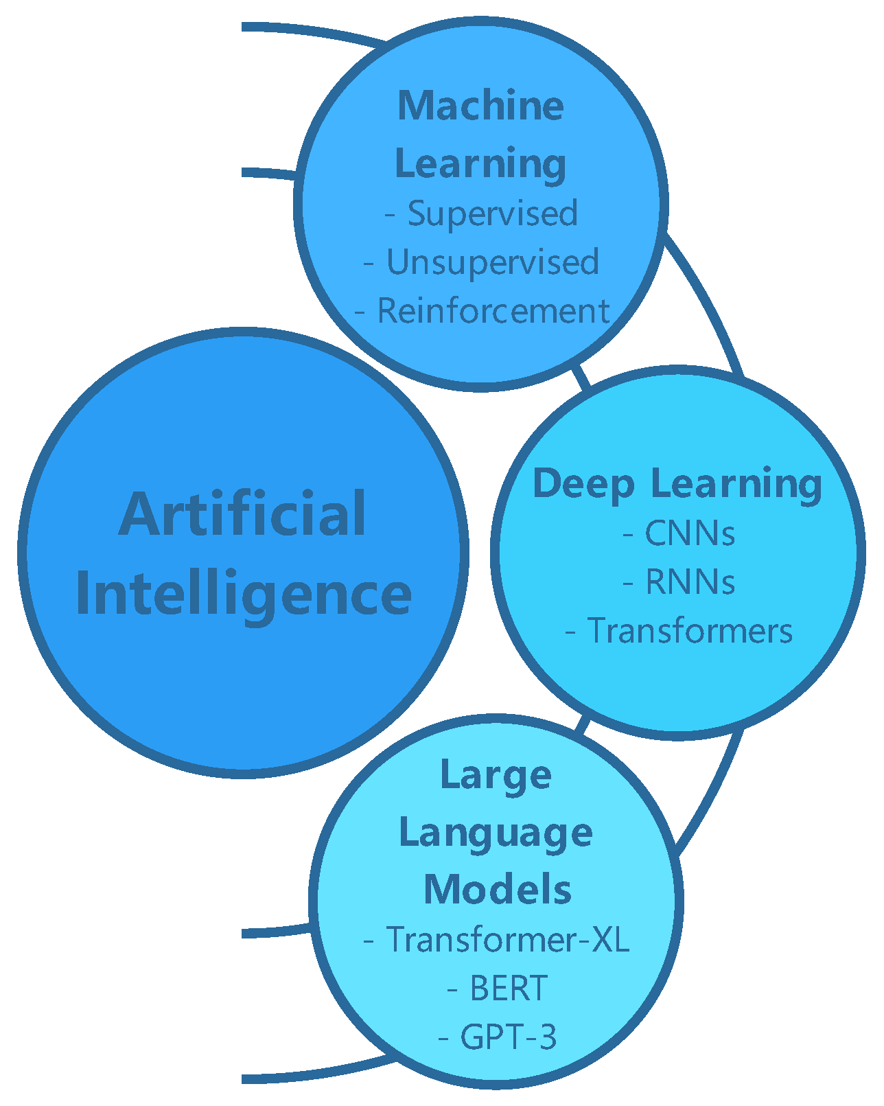
Figure 2.
Machine Learning, Deep Learning, and Large Language Model Processes
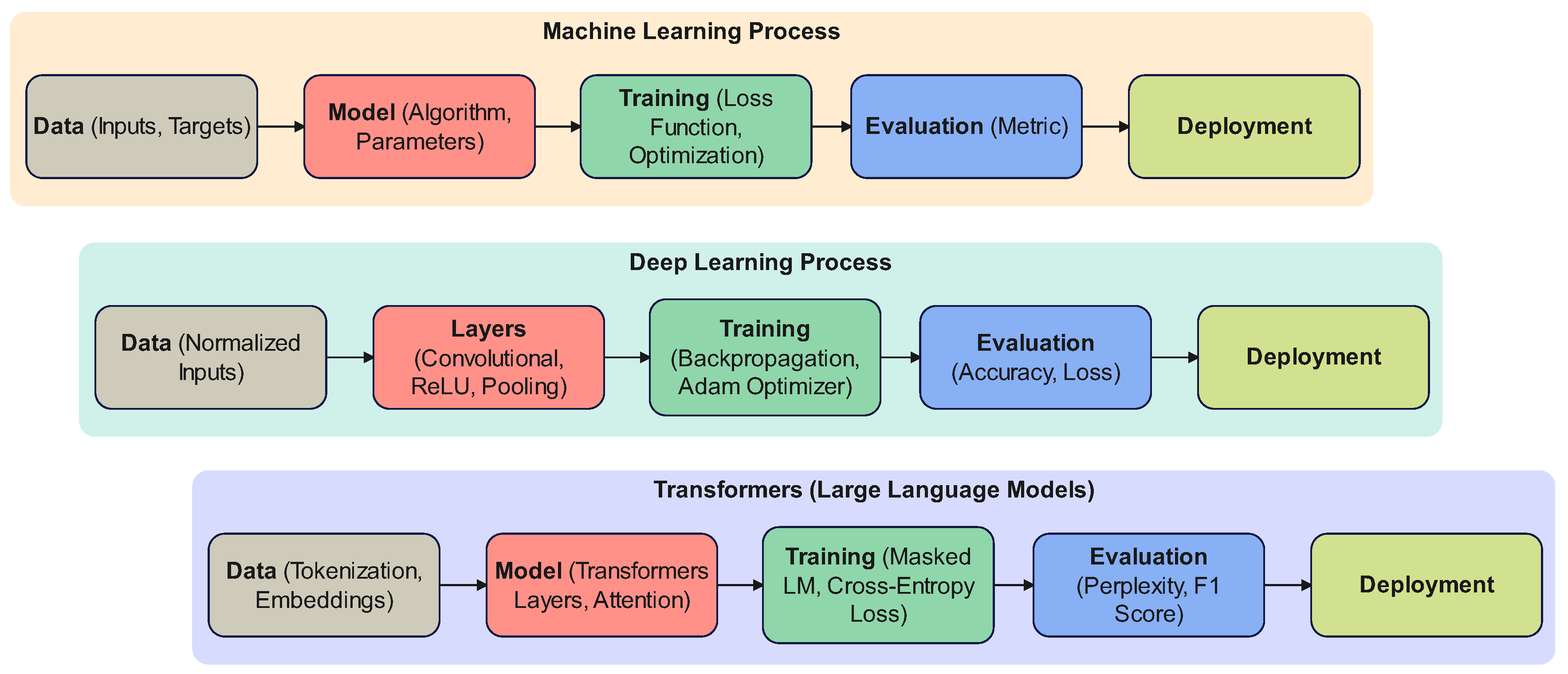
Figure 4.
Flamingo Multimodal Modal
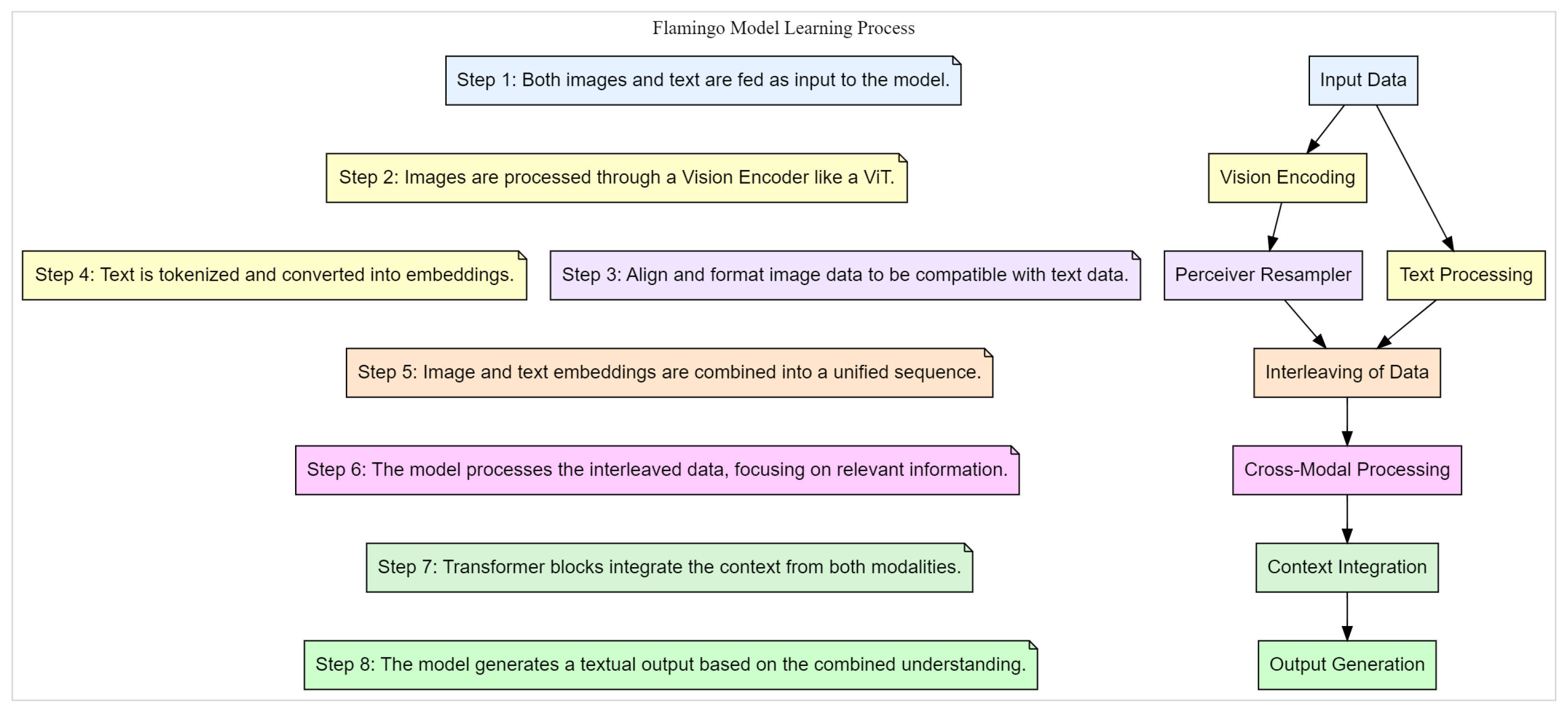
Figure 5.
Overview of model-specific interpretability techniques: This diagram categorizes interpretability methods based on different machine learning models, including Reinforcement Learning, Clustering & Unsupervised Models, Transformers, Ensemble Models, Bayesian Models, Neural Networks (Deep Learning Models), Support Vector Machines (SVMs), Linear & Logistic Regression, and Tree-Based Models. Each category outlines specific interpretability techniques, such as policy visualization for reinforcement learning, token contribution analysis for transformers, saliency maps for neural networks, and feature contribution for tree-based models, providing tailored insights for each model type
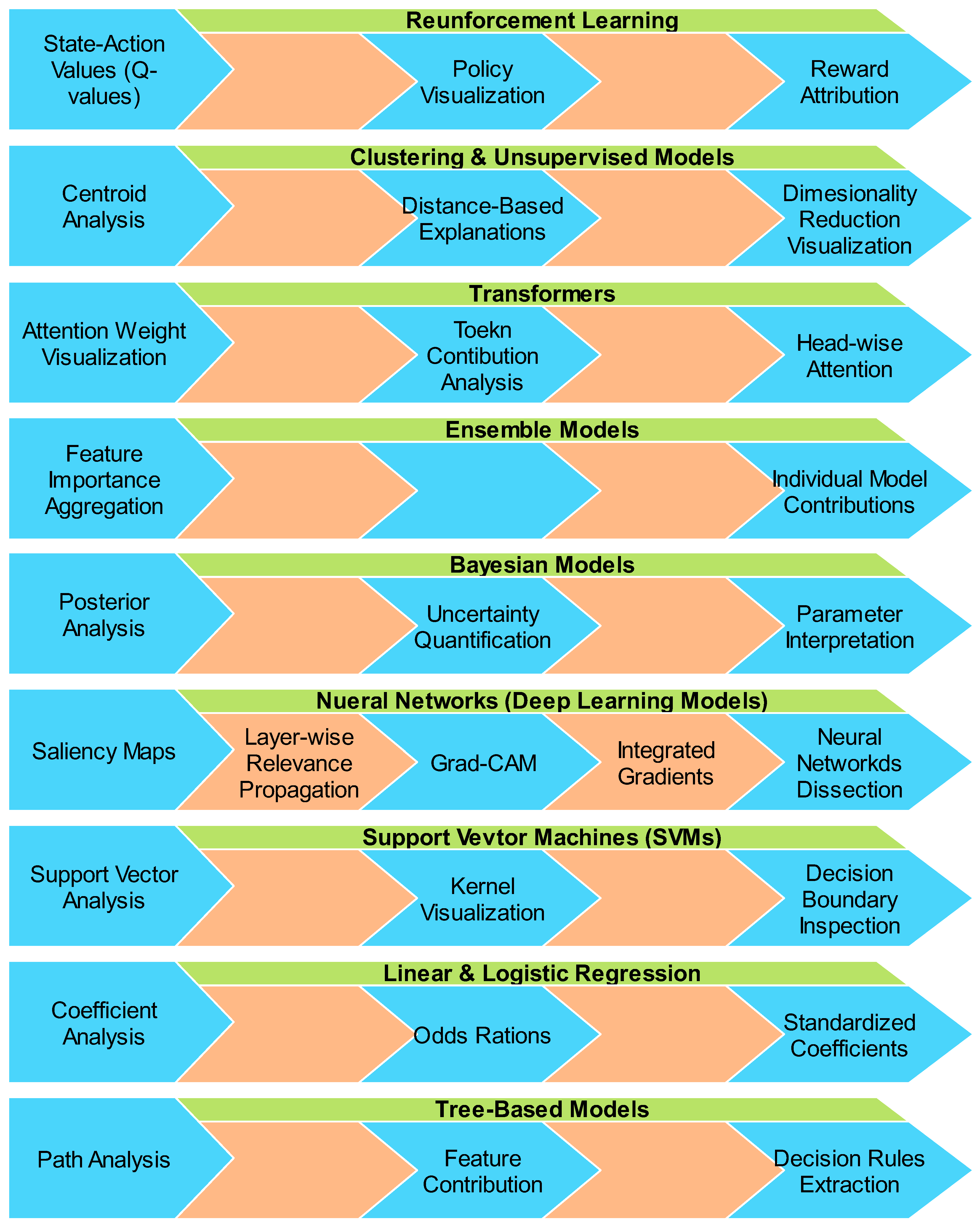
Figure 6.
Overview of model-agnostic interpretability techniques for machine learning: The flow diagram outlines six methods—Surrogate Models, Feature Importance, Individual Conditional Expectation (ICE), Partial Dependence Plots (PDP), SHAP (SHapley Additive exPlanations), and LIME (Local Interpretable Model-agnostic Explanations)—showing their input, process, and output in interpreting and explaining machine learning model predictions.
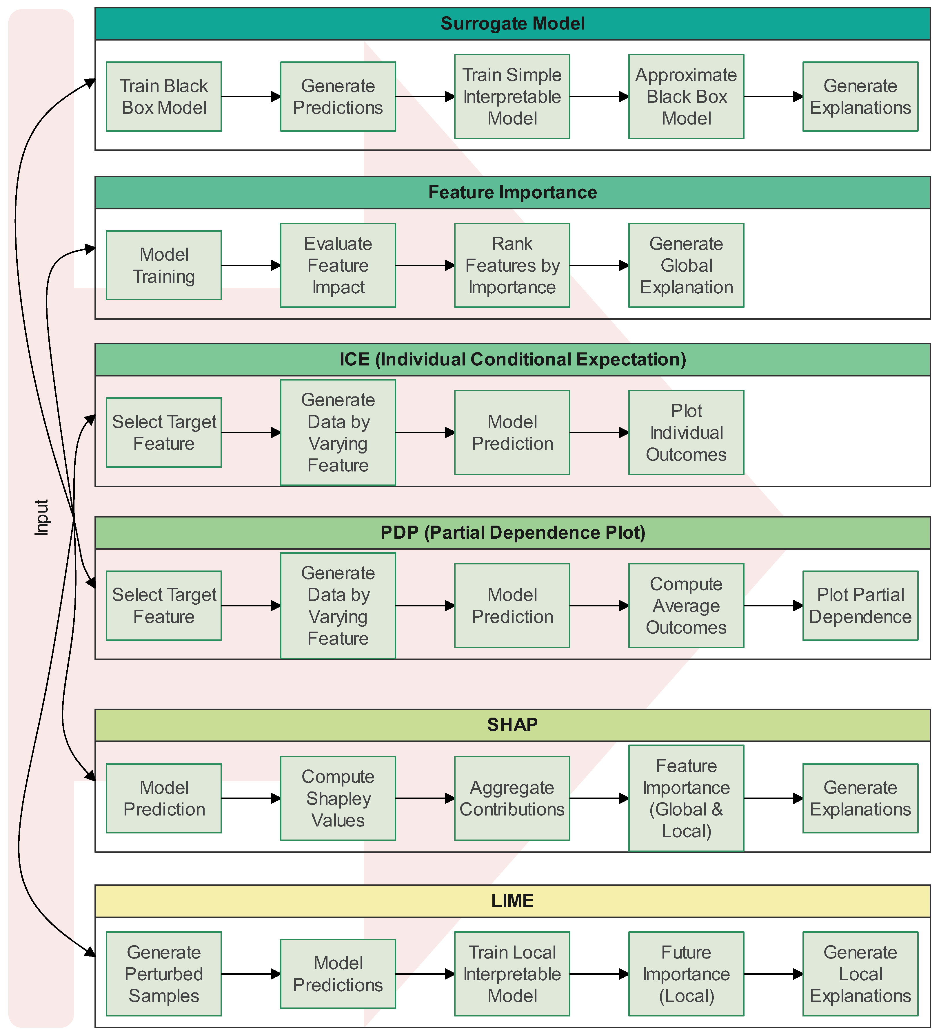
Figure 7.
Post-hoc explainability methods for machine learning models: The diagram presents various techniques including Gradient-Based Methods (e.g., Grad-CAM), Local Surrogate Models (e.g., LIME), Global Surrogate Models, Individual Conditional Expectation (ICE), Partial Dependence Plots (PDP), Attention Mechanisms, Saliency Maps, Counterfactual Explanations, and Feature Attribution (e.g., SHAP, LIME). Each method is broken down into a sequential process, illustrating how inputs are transformed into meaningful explanations for interpreting model behavior and predictions
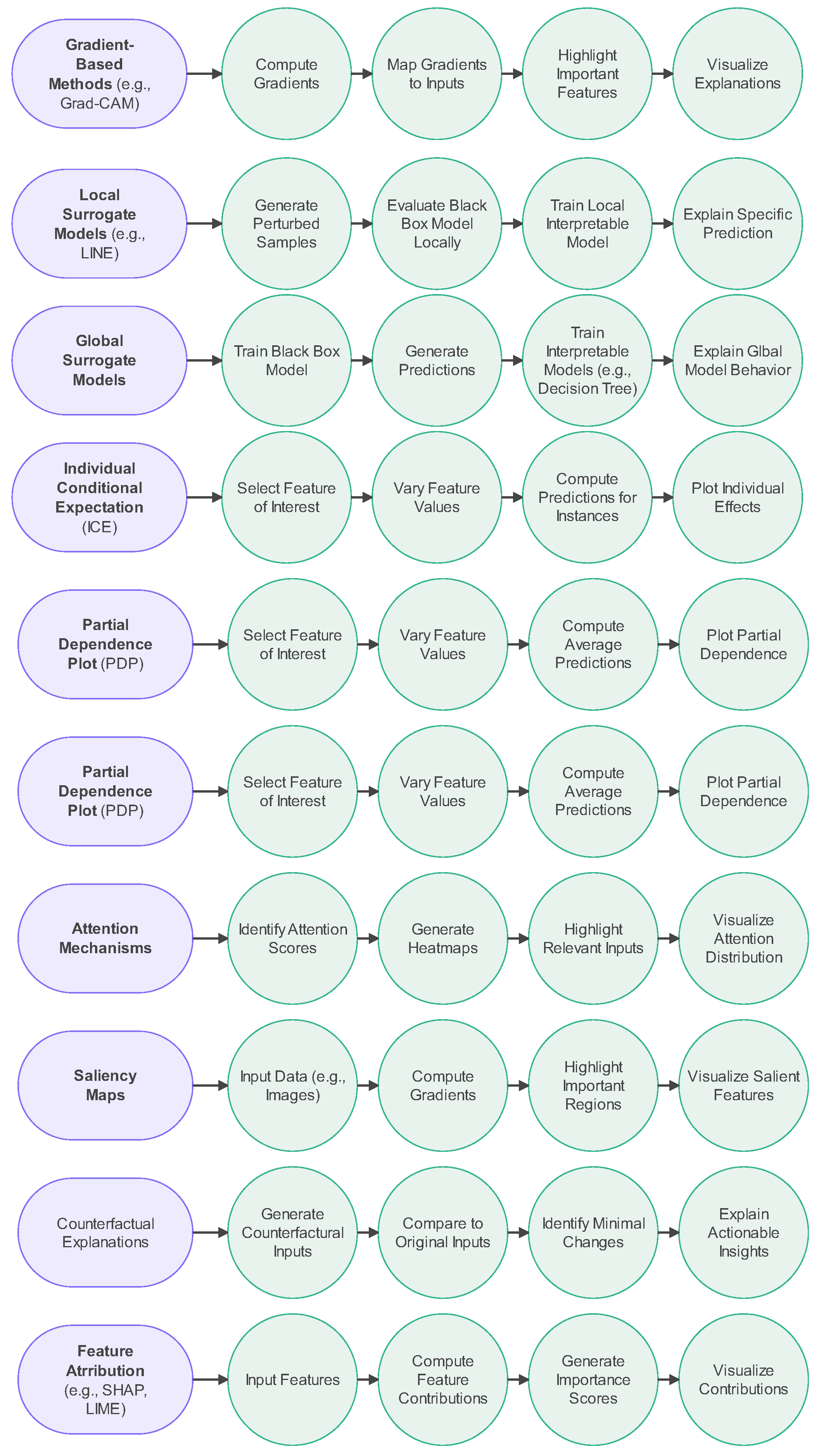
Figure 8.
Hierarchy of Explainable AI in Robotics
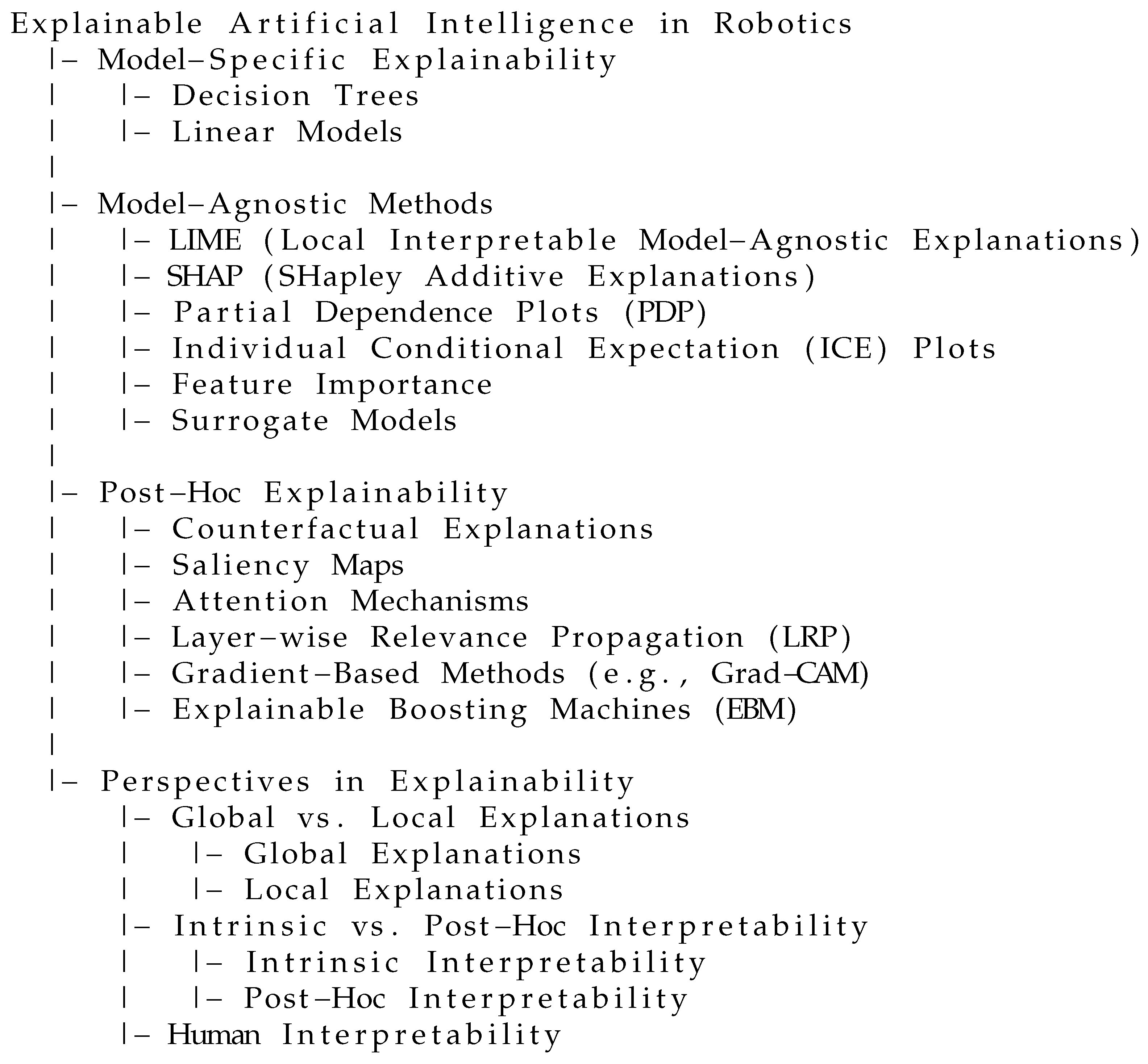
Table 5.
Comparison of Decision Trees and Linear Models Based on Interpretability and Performance
| Name of the Algorithm | Popularity | Mathematical Representation | Short Description | Benefits | Problems | What is Different from Other Methods | Overall Performance by Other Researchers |
|---|---|---|---|---|---|---|---|
| Decision Trees: Intrinsically interpretable | High | N/A | Decision Trees are popular machine learning models due to their ease of interpretability. The tree-like structure provides a clear decision path from root to leaf, making the decision-making process easily understandable. | The main advantage is the transparency of their decisions, which aids in building trust, explaining the model, and identifying biases. | Decision trees can overfit to training data, leading to poor generalization on new data. They are also sensitive to small changes in data, which can result in different tree structures, causing instability. | Unlike black-box models like neural networks, decision trees are fully interpretable, allowing users to trace the decision path directly from root to leaf, showing how each feature impacts the prediction. | Decision trees perform well in simple cases but may not achieve the same level of accuracy as more complex models (e.g., random forests, deep learning) in tasks with higher complexity. |
| Linear Models: Coefficients provide direct interpretability | Moderate | N/A | Linear models offer a simple way to model relationships between variables by quantifying the impact of each predictor on the response variable through coefficients. This makes them highly interpretable and suitable for applications requiring clear insights into data patterns. | The ability to clearly quantify and explain the influence of each predictor variable on the outcome simplifies understanding and interpretation of relationships in the data. | Linear models assume linear relationships between variables, which may not always capture the true complexity of non-linear relationships in real-world data, limiting their applicability to more complex tasks. | Linear models differ from others in their explicit representation of predictor variables through easily interpretable coefficients, making them highly transparent and easy to understand. | Researchers appreciate their simplicity, transparency, and ease of interpretation, though their performance may vary depending on the complexity of the data. They are often used in cases where interpretability is crucial. |
Table 6.
Comparison of Machine Learning Interpretability Techniques
| Name of the Algorithm | Popularity | Mathematical Representation | Short Description | Benefits | Problems | What is Different from Other Methods | Overall Performance by Other Researchers |
|---|---|---|---|---|---|---|---|
| LIME (Local Interpretable Model-agnostic Explanations) | High | N/A | LIME is used to explain predictions from black-box machine learning models. It approximates complex models locally around a specific prediction using simpler models, enabling users to understand key factors driving predictions. | It is model-agnostic, meaning it works with any machine learning model. It is versatile and can explain opaque models, providing insights otherwise inaccessible. | LIME offers local explanations, which means it explains individual predictions without offering a global view of the model’s behavior. This can lead to misleading conclusions about overall model behavior. | LIME approximates black-box models by creating simple, interpretable models (e.g., linear models) locally around specific predictions, rather than interpreting the entire model globally. | LIME is widely regarded as a valuable tool for explaining individual predictions, but researchers caution that its local nature may not represent the model’s global behavior accurately. |
| SHAP (SHapley Additive exPlanations) | High | N/A | SHAP uses game theory to fairly distribute the contribution of each feature to a prediction, offering insights into feature importance and model behavior. | SHAP provides a theoretically sound, unified approach to explaining predictions, improving upon prior methods that lacked consistency. | Calculating exact SHAP values can be computationally expensive, especially for large datasets and complex models, although approximations can help. | SHAP unifies various feature importance methods by providing a solid theoretical foundation, which clarifies and connects other techniques in the field of model interpretability. | SHAP is highly regarded for its theoretical grounding and practical application, although the computational cost remains a challenge, especially for complex models. |
| Partial Dependence Plots (PDP) | High | N/A | PDPs visualize the marginal effect of one or two features on a predicted outcome, showing if the relationship between a feature and the target is linear, complex, or non-existent. | PDPs effectively illustrate the marginal effect of features, providing clear visual insights into model behavior. | PDPs can be misleading when predictor variables are correlated, which may distort the interpretation of individual feature effects. | PDPs visualize the average effect of features on outcomes, marginalizing the effects of other features, offering insights into model behavior in a simplified form. | Researchers find PDPs useful but emphasize caution, especially with complex datasets that have feature dependencies. They should not be used in isolation. |
| Individual Conditional Expectation (ICE) Plots | Moderate | N/A | ICE plots visualize the relationship between a feature and the model’s prediction for individual observations, offering instance-level insights. | ICE plots illustrate how predictions for individual observations change as a feature varies, while keeping other features constant, offering granular insights. | ICE plots can become visually cluttered with large datasets, obscuring overall trends, making them difficult to interpret when many observations are involved. | ICE plots show feature dependency on an individual basis, differing from PDPs which show average effects across the dataset. | ICE plots are recognized for offering detailed individual-level insights, but researchers caution against visual clutter and difficulty in interpreting plots with many observations. |
| Feature Importance | High | N/A | Assigns scores to features based on their contribution to the model’s prediction accuracy, offering insights into which features are most influential. | Feature importance helps in understanding which features drive predictions, guiding feature selection and improving model interpretability. | Different feature importance methods can yield inconsistent rankings, making it challenging to determine the true importance of features. | Feature importance accounts for feature interactions and non-linear relationships, offering a comprehensive view of feature influence. | While feature importance is valuable for model understanding, researchers note that results can be misleading due to feature correlations and model instability. |
| Surrogate Models | Moderate | N/A | Surrogate models are simplified approximations of complex systems or simulations, reducing computational costs for prediction and analysis. | Surrogate models significantly reduce computational time and costs, making tasks like optimization and uncertainty quantification more feasible. | Surrogates are only approximations and may not fully capture the complexities of the original system, potentially leading to inaccuracies. | Surrogate models replace complex simulations with faster, data-driven approximations, making them useful for handling expensive evaluations. | Surrogate models show good agreement with detailed simulations but depend heavily on model type, training data quality, and application, influencing their effectiveness. |
Table 7.
Comparison of Machine Learning Interpretability Techniques
| Name of the Algorithm |
Popularity | Mathematical Representation |
Short Description | Benefits | Problems | What is Different from Other Methods |
Overall Performance by Other Researchers |
|---|---|---|---|---|---|---|---|
| Counterfactual Explanations | High | N/A | Counterfactual explanations provide what-if scenarios to show how changing specific input features would alter a model’s prediction. | Helps users understand which input variables are most influential and how to achieve desired outcomes by adjusting certain features. | It can be difficult to generate realistic counterfactuals, especially for complex models, making practical application challenging. | Focuses on explaining how an outcome can be changed rather than why the current decision was made. | More research is needed to improve the feasibility and practicality of using counterfactual explanations across diverse applications. |
| Saliency Maps | High | N/A | Visual representations that highlight important pixels in an image, showing which parts of an image contribute most to a deep learning model’s prediction. | Provides insights into convolutional neural networks’ decision-making process by focusing on the most relevant image areas. | Sensitive to noise and can produce inconsistent explanations without standardized evaluation metrics. | Offers pixel-level visual explanations for image-based models, providing intuitive insights that distinguish it from other methods. | Researchers recognize their value but emphasize caution in interpretation and the need for more robust evaluation metrics. |
| Attention Mechanisms in Neural Networks | High | N/A | Inspired by human visual attention, attention mechanisms allow networks to focus selectively on important parts of the input data, improving performance. | Enhances neural network performance by concentrating on the most relevant input features for better efficiency and prediction accuracy. | Increased computational cost due to the additional complexity introduced by attention mechanisms, especially in large datasets. | Enables neural networks to process input more efficiently by focusing on relevant data rather than treating all inputs equally. | Researchers widely agree that attention mechanisms improve performance significantly, especially in tasks involving sequential data. |
| Layer-wise Relevance Propagation (LRP) | Moderate | N/A | Decomposes neural network outputs back to input features to interpret decisions, showing which input parts contribute most to a prediction. | Enhances interpretability by revealing which parts of the input are most relevant for a model’s decision, applicable across various types of neural networks. | High computational complexity for large models, and explanations may not always align with human intuition. | Provides layer-specific, detailed explanations by backpropagating relevance scores, offering more granular insights than other methods. | Researchers appreciate its ability to provide intuitive explanations but highlight the need for improvements in computational efficiency and interpretability. |
| Gradient-Based Methods (e.g., Grad-CAM) | High | N/A | Use gradients flowing into convolutional neural networks to visualize which image regions are important for a particular prediction. | Provides visual explanations that make convolutional neural networks more transparent and interpretable, particularly for image-based tasks. | Can lack fine-grained detail, highlighting broad regions but missing subtle image features that may also influence decisions. | Broadly applicable across different CNN architectures without requiring retraining, making it versatile for understanding various models. | Researchers view Gradient-Based Methods like Grad-CAM as valuable for explaining CNNs, although improvements in detail are still needed. |
| Explainable Boosting Machines (EBM) | High | N/A | Combines boosting techniques with generalized additive models, balancing accuracy and interpretability by providing high-quality predictions while remaining understandable. | High accuracy with clear interpretability, allowing users to understand how predictions are made without sacrificing prediction performance. | Model complexity increases significantly with high-dimensional data, potentially challenging the interpretability of EBMs. | Balances accuracy and interpretability, unlike many models that prioritize one over the other (e.g., neural networks for accuracy or decision trees for simplicity). | Researchers report state-of-the-art accuracy comparable to less interpretable models like Gradient Boosting Machines while maintaining ease of understanding. |
Table 11.
Comparison of Different Machine Learning Interpretability Techniques
| Name of the Algorithm |
Popularity | Mathematical Representation |
Short Description | Benefits | Problems | What is Different than Other Methods |
Overall Performance by Other Researchers |
|---|---|---|---|---|---|---|---|
| Saliency maps | High | Saliency maps calculate the magnitude of the gradient of a model’s output with respect to each input pixel, highlighting areas with higher influence on the output. | They highlight the important regions in an image for a deep learning model’s prediction, enhancing interpretability in image-based tasks. | Can be noisy and difficult to interpret. Sometimes highlight irrelevant features and may not fully reflect the model’s decision-making process. | Rely on back-propagation gradients and are specific to the model, often used for CNN-based image models. | Despite improvements in speed and accuracy, saliency maps are still outperformed by models designed specifically for salient object detection. | |
| Attention mechanisms | High | N/A | Attention mechanisms enable models to focus on specific parts of the input by assigning different weights to parts of the data, highlighting the most relevant information. | Improve both the effectiveness and interpretability of models, especially in tasks like machine translation and image captioning. | High computational cost, sensitivity to input ordering, and difficulty in training. Can still be considered a "black box." | Dynamically prioritize information, leading to improved performance in various deep learning tasks, especially with sequential data. | Researchers consistently report positive results, with attention mechanisms significantly improving the performance of models across many applications. |
| Natural language explanations | Moderate | N/A | Provide human-understandable explanations by expressing the AI’s decision-making process in natural language, similar to explaining reasoning to a human colleague. | Help bridge the gap between AI decision-making and human understanding, making AI systems more accessible and transparent. | Challenges include generating accurate, contextually relevant explanations that balance clarity and technical depth. | Unlike other methods that rely on visualizations or rule-based explanations, this approach uses everyday language to communicate reasoning. | This is an evolving area, with more research needed to improve the quality of explanations and assess its practical adoption across various fields. |
Disclaimer/Publisher’s Note: The statements, opinions and data contained in all publications are solely those of the individual author(s) and contributor(s) and not of MDPI and/or the editor(s). MDPI and/or the editor(s) disclaim responsibility for any injury to people or property resulting from any ideas, methods, instructions or products referred to in the content. |
© 2025 by the authors. Licensee MDPI, Basel, Switzerland. This article is an open access article distributed under the terms and conditions of the Creative Commons Attribution (CC BY) license (http://creativecommons.org/licenses/by/4.0/).
Copyright: This open access article is published under a Creative Commons CC BY 4.0 license, which permit the free download, distribution, and reuse, provided that the author and preprint are cited in any reuse.


