
Submitted:
18 January 2025
Posted:
20 January 2025
You are already at the latest version
Abstract
This study investigates the application of modified Wasserstein Generative Adversarial Networks with Gradient Penalty (WGAN-GP) to generate synthetic RGB and infrared (IR) datasets for precision agriculture, particularly targeting the detection of Raphanus Raphanistrum (wild radish). Traditional WGAN models face challenges such as vanishing gradients and poor convergence, which hinder their effectiveness in generating high-quality synthetic data. To address these issues, this work proposes modifications that include replacing fully connected layers with convolutional and transposed convolutional layers, combined with batch normalization, to improve the fidelity of generated images and training stability. The experimental results demonstrate that the modified WGAN-GP produces superior synthetic images compared to other GAN variants, especially in maintaining structural similarity for RGB datasets. However, generating high-quality IR images remains challenging due to inherent spectral complexities, with consistently lower SSIM (Structural Similarity Index) scores across models. This study highlights the importance of architectural modifications and auxiliary learning strategies in enhancing GAN performance, especially for complex agricultural datasets. The findings suggest that future work should focus on integrating attention mechanisms and advanced loss functions to further improve model stability and the quality of generated synthetic data. These advancements are vital for the broader adoption of GANs in precision agriculture, enabling enhanced data augmentation for machine learning applications that support effective crop monitoring and management.
Keywords:
Generative Adversarial Network (GAN)
; Wasserstein Generative Adversarial Network (WGAN)
; Gradient Penalty (GP)
; Infrared (IR)
; Raphanus Raphanistrum
1. Introduction
Raphanus Raphanistrum, commonly known as wild radish, presents a significant challenge in precision agriculture due to its aggressive nature and adaptability. This weed competes vigorously with crop plants for essential resources such as water, nutrients, and sunlight, which can lead to substantial reductions in crop yield and quality (Heap, 2014). It is particularly problematic in the early stages of crop development when its rapid growth can quickly overshadow crops, inhibiting their growth and establishment (Boutsalis et al., 2012). Furthermore, this invasive species has developed resistance to multiple classes of herbicides, including Acetolactate Synthase (ALS) inhibitors, Photosystem II inhibitors (PSII), and synthetic auxins, making chemical control strategies increasingly ineffective (Walsh, Owen, & Powles, 2007; Owen et al., 2015). This resistance complicates weed management in precision agriculture, where the goal is to minimize herbicide use and environmental impact.
Additionally, wild radish has a high reproductive capacity, producing numerous seeds that can persist in the soil seed bank for several years (Cheam & Code, 1995). This long-term seed viability means that even a few uncontrolled plants can lead to significant reinfestation, necessitating continuous monitoring and intervention. Its adaptability to a range of soil types and climates further exacerbates the problem, allowing it to thrive in diverse agricultural settings (Llewellyn & Powles, 2001). From a technological perspective, wild radish also poses a challenge to precision agriculture tools such as spectral imaging and UAV-based weed detection systems. Its morphological characteristics and growth patterns can complicate accurate differentiation from crop plants, reducing the effectiveness of automated detection and intervention systems (Rueda-Ayala, Peña, and Höglind 2019).
Wild radish can also interfere with harvesting operations, leading to increased wear on machinery and contamination of crop yields, which is particularly problematic in cereal crops where seed purity is critical (Gill & Bowran, 2000). These combined factors contribute to the high economic costs associated with managing wild radish infestations, including increased expenditures on herbicides, specialized equipment, and labor (Walsh, Owen, & Powles, 2007). As a result, wild radish is considered one of the most problematic weeds in precision agriculture, necessitating integrated weed management strategies that combine mechanical, chemical, and cultural control measures (Borger et al., 2012).
Furthermore, Raphanus raphanistrum’s ability to cross-pollinate with herbicide-tolerant crops such as canola complicates its management, as it can gain herbicide resistance through gene flow (Kebaso et al., 2020). The weed’s rapid spread is often aided by human activities, allowing it to quickly colonize new areas and disrupt local ecosystems and agricultural productivity (Barnaud et al., 2013). Consequently, Raphanus raphanistrum is not just a persistent weed but a significant agricultural challenge that necessitates a combination of integrated weed management strategies to effectively mitigate its impact effectively.
Annotating weeds such as Raphanus raphanistrum in RGB and multispectral proximal agricultural images presents a time and cost complexity due to a combination of environmental and technical factors. The environmental factor is based on the visual similarity between weeds and crops as both share similar colors and textures, particularly in RGB images, making it hard to be distinguished between them based solely on visual cues. This issue is compounded by the morphological variability of wild radish, which can exhibit a wide range of shapes and sizes, sometimes mimicking the appearance of crop plants. The complex backgrounds in agricultural settings add another layer of complexity. Soil, crop residues, and other organic matter create cluttered scenes, making it difficult to isolate weeds from their surroundings. Additionally, interference from other vegetation, including other weed species or volunteer crops, leads to overlapping or intertwined plants that obscure the features of the target weed (Rana et al., 2024).
Generative Adversarial Networks (GANs) have shown significant utility in image augmentation for weed detection and segmentation, providing robust datasets for training machine learning models when the availability of annotated weed images is limited. GANs consist of two neural networks - the generator and the discriminator, working simultaneously (Figure 1). The generator creates synthetic images that resemble the target dataset, while the discriminator attempts to distinguish between real and generated images. This adversarial process enables GANs to produce high-quality, realistic images that can be used to augment datasets (Goodfellow et al., 2014). In the context of weed detection and segmentation, GANs offer several benefits.
Firstly, they can generate diverse and realistic weed images, which address the common issue of data scarcity in agricultural datasets. When training deep learning models for weed detection, having a large and varied dataset is crucial for improving model robustness and generalization (Mokhtar et al., 2021). GANs can simulate different growth stages, lighting conditions, and plant morphologies, thus increasing the variability of training images. This enhanced variability helps models learn to recognize weeds under various conditions, reducing overfitting and increasing the model’s ability to perform well in real-world scenarios. Secondly, GANs facilitate the generation of annotated synthetic images, which are particularly useful for segmentation tasks. Using architectures like Pix2Pix or CycleGAN, synthetic images can be created along with corresponding pixel-level annotations, making them highly valuable for training segmentation models (Isola et al., 2017; Zhu et al., 2017). This capability is essential because manual annotation of images for segmentation is time-consuming and labor-intensive, especially when dealing with complex weed-crop environments.
Moreover, GANs can also be used to enhance the domain adaptation process, which is necessary when a model trained on one dataset (e.g., laboratory or simulated data) needs to be applied to a different domain (e.g., field images). GAN-based domain adaptation techniques can help transform synthetic images to resemble real-world field conditions, bridging the gap between different datasets and improving model performance across domains (Hussain et al., 2020). Another critical application of GANs in weed detection is addressing class imbalance. Weed datasets often suffer from an imbalance where certain weed classes are underrepresented. GANs can generate synthetic images of these underrepresented classes, providing a more balanced dataset for training. This class-balancing effect can lead to more equitable detection and classification performance across different weed species (Huang et al., 2020). Overall, GANs significantly enhance image augmentation for weed detection and segmentation by generating diverse, high-quality synthetic data, facilitating pixel-level annotations, aiding domain adaptation, and addressing class imbalance. These capabilities lead to more robust and generalized models that can perform well in diverse agricultural settings.
Wasserstein Generative Adversarial Networks (WGANs) have emerged as a robust method for generating high-quality synthetic data by incorporating the Wasserstein distance in the loss function, which improves stability and training convergence. However, traditional WGANs face gradient vanishing and exploding issues, hindering their training. To address these, the Wasserstein GAN with Gradient Penalty (WGAN-GP) was introduced (Arjovsky, Chintala, and Bottou 2017), replacing weight clipping with a gradient penalty to ensure the Lipschitz constraint on the discriminator network. This leads to more stable training and superior data quality (Cui and Jiang 2017), making suitable for augmenting datasets in agricultural monitoring (Yang and Wang 2020). WGAN-GP effectively synthesizes both RGB and multispectral images, enhancing datasets for precision farming applications (Zhao et al., 2020). These synthetic images improve the performance and generalizability of machine learning models, particularly in data-limited scenarios (Hazra et al. 2022).
Despite these advantages, WGAN-GP still faces significant limitations. GANs with gradient penalties suffer from mode collapse and training instability, especially with complex or high-dimensional data distributions (Tan et al., 2020). The gradient penalty increases computational overhead, slowing training and complicating the process for larger datasets or more complex architectures (Liu & Qiu, 2020). Additionally, while intended to enforce Lipschitz continuity, the gradient penalty is not always precise, and alternative methods like spectral normalization may offer more effective solutions (Cui & Jiang, 2017). The use of gradient penalties can also limit the discriminator’s capacity, reducing its ability to differentiate between real and generated data, thus affecting output quality (Liu, 2018). Furthermore, WGAN-GP may solve a different optimal transport problem than intended, leading to unexpected behaviors and complicated training dynamics (Milne & Nachman, 2021).
Traditional WGAN-GP architecture often suffers from mode collapse and limited fidelity when dealing with complex datasets. The modifications presented in this study address these issues for RGB datasets by transitioning from fully connected layers to convolutional layers and incorporating transposed convolutions for upsampling. These changes enhance the model’s ability to capture and preserve spatial relationships, producing images with clearer edges, more accurate textures, and higher fidelity. The addition of batch normalization further stabilizes the training process, enabling the generator to create outputs that closely resemble original data. However, these improvements highlight the need for additional parametric modifications to handle more challenging data types like IR images, which exhibit greater spectral variability and complexity.
The modular design of the modified WGAN-GP architecture ensures its adaptability to a wide range of agricultural datasets, including those with varying species or imaging modalities. This flexibility positions it as a scalable and effective solution for generating high-quality synthetic data across diverse applications, with future iterations aimed at refining performance for both RGB and IR spectra.
2. Materials and Methods
2.1. Dataset
Multiple leaf-bound instances were clipped from the 12 January 2022 RGB and 13 January 2022 Red Edge bands to constitute two classes of data towards training the Wasserstein GAN with Gradient Penalty (Rana et al., 2024). A few clipped samples from the datasets are demonstrated in Figure 2(c) and 2(d).
2.2. Methodology
2.2.1. Data Preparation
a) Image Collection and Preprocessing
RGB images: A total of 57 RGB images were acquired on 12 January 2022. 876 leaf- bound samples were clipped in the order of 155 x 115 pixels containing the periphery of Raphanus Raphanistrum. The acquisition sensor was Canon 2000D and the sensing altitude was 1m.
Infrared images: A total of 202 Infrared images were acquired on 13 January 2022. 850 leaf-bound samples were clipped in the order of 155 x 115 pixels containing the periphery of Raphanus Raphanistrum. The acquisition sensor was Micasense RedEdge – M and the sensing altitude was 1m.
Data splitting: RGB and IR images were split into training (80%) and testing (20%).
b) Image Normalization
Image normalization is a critical preprocessing step for training neural networks, including generator networks, and it involves scaling pixel values to a common range to improve convergence and stability. For RGB images, normalization typically involves rescaling pixel values from their original range (e.g., 0-255) to a range of 0-1 or -1 to 1. This can be done by dividing the pixel values by 255 for a 0-1 range, or by first rescaling to 0-1 and then shifting and scaling to achieve a -1 to 1 range. Additionally, channel-wise mean subtraction is commonly performed, where the mean and standard deviation for each channel (R, G, B) are computed from the training dataset. Each pixel value in a channel is then subtracted by the channel’s mean and divided by the channel’s standard deviation (Pal & Sudeep, 2016; Pontalba et al., 2019).
For Multispectral (MS) images, the normalization techniques are similar but must account for the additional spectral bands beyond the standard RGB channels. MS images’ pixel values are also rescaled to a range of 0-1. Band-wise normalization involves calculating the mean and standard deviation for each spectral band across the entire training dataset and then normalizing each band separately by subtracting its meaning and dividing by its standard deviation. Min-max normalization is another common approach for MS images, particularly useful for bands with varying value ranges, where each band is scaled to the 0-1 range based on its minimum and maximum values (Liyanage et al., 2020; Melgarejo et al., 2016; Chen et al., 2014).
2.2.2. Rationale for Network Modifications
The proposed modifications to the WGAN-GP architecture aim to address common challenges in GAN training, such as mode collapse, vanishing gradients, and unstable convergence.
Gradient Penalty: The inclusion of a gradient penalty enforces the Lipschitz constraint on the discriminator, stabilizing training by smoothing the optimization landscape. This eliminates the need for weight clipping, which can overly restrict the model’s capacity (Gulrajani et al., 2017). The gradient penalty requires retainment in the discriminator to enforce the Lipschitz constraint, which is crucial for stabilizing the adversarial training process. In the modified architecture, the penalty will be applied in conjunction with convolutional layers to enhance its effectiveness for spatially structured data such as RGB and IR images.
Convolutional Layers: Replacing fully connected layers with convolutional layers preserves spatial relationships in the image data, a critical factor in generating high-quality synthetic images. This design enhances the model’s ability to capture and replicate fine structural details (Radford et al., 2015). In the generator, fully connected layers will be replaced with convolutional and transposed convolutional layers to enhance spatial feature preservation. These transposed convolutions need to be configured with a filter size of 4x4, a stride of 2, and same padding to ensure artifact-free upsampling. Batch normalization will be applied to stabilize training and improve convergence. In the discriminator, multi-layer convolutional architecture with Leaky ReLU activation and dropout need to be implemented to improve feature extraction and prevent overfitting.
Transposed Convolutions: Used for upsampling, transposed convolutions ensure that generated images maintain a coherent structure, avoiding artifacts commonly seen with simpler upsampling techniques (Odena et al., 2016). The generator network requires transposed convolutions to progressively upsample feature maps from a low-resolution latent space to the final image resolution. Each transposed convolution layer needs to employ 4x4 filters, a stride of 2, and same padding to ensure spatial consistency and reduce artifacts. Batch normalization and ReLU activation would be applied after each layer to stabilize training and enhance feature generation. The final layer to be used is Tanh activation to normalize pixel values to the range [-1, 1]
Batch Normalization: Batch normalization stabilizes training by normalizing feature distributions, reducing internal covariate shifts, and improving convergence (Ioffe & Szegedy, 2015). The integration of this function in the generator will improve the training stability, which will be evidenced by smoother convergence in the loss curves. Generated images would be demonstrating higher structural fidelity and reduced artifacts, particularly in RGB datasets. The decision to omit batch normalization in the discriminator will ensure the gradient penalty’s effectiveness, preserving the model’s stability.
2.2.3. Model Design
a) Generator Network
The generator network in the updated Wasserstein GAN with Gradient Penalty (WGAN-GP) is designed to produce RGB images from random noise (Table 1). It begins with a fully connected layer that transforms the 100-dimensional latent vector into a 128×7×7 feature map using the ReLU activation function for non-linearity. This feature map is then reshaped into a 7x7x128 format and undergoes a series of upsampling operations via transposed convolution layers. The first transposed convolution layer applies 128 filters of size 4x4 with a stride of 2 and same padding, doubling the spatial dimensions to 14x14 while maintaining a depth of 128. Batch normalization is used to stabilize and speed up training, followed by ReLU activation. The second transposed convolution layer further upsamples the feature map to 28x28 with 64 filters of size 4x4, again followed by batch normalization and ReLU activation. The final output layer is a convolutional layer with 3 filters (for RGB) of size 4x4 and same padding, using the Tanh activation function to scale pixel values to the range [−1, 1]. This configuration enables the generator to produce high-quality RGB images that closely resemble the real images in the training dataset.
b) Discriminator Network
The discriminator network in this WGAN – GP is designed to differentiate between real RGB images and those generated by the generator. It begins with a convolutional layer that applies 16 filters of size 3x3 with a stride of 2 and same padding, reducing the spatial dimensions while preserving the depth. This layer uses the Leaky ReLU activation function to handle negative values and a dropout layer to prevent overfitting. The subsequent convolutional layer applies 32 filters of size 3x3 with a stride of 2 and same padding, followed by batch normalization, Leaky ReLU activation, and another dropout layer. The third convolutional layer further reduces the spatial dimensions using 64 filters of size 3x3 with a stride of 2 and same padding, again followed by batch normalization, Leaky ReLU activation, and dropout. The final convolutional layer applies 128 filters of size 3x3 with a stride of 1 and same padding, followed by batch normalization and Leaky ReLU activation. This results in a deep feature map which is then flattened and passed through a fully connected layer to produce a single output value. This architecture enables the discriminator to effectively learn the features that distinguish real images from fake ones generated by the generator, providing accurate feedback to improve the generator’s performance during training.
2.2.4. Training the WGAN
The training begins with the careful setting of hyperparameters. The latent dimension, which represents the input noise vector’s size for the generator, is typically set to 100, allowing for a sufficient level of complexity in the generated images. A batch size of 32 is selected to balance memory usage and training stability, and the training process is set to continue for a maximum of 50 epochs, ensuring ample opportunity for the network to learn. The learning rate is fixed at 0.00005 to ensure gradual and stable updates to the network parameters, while the discriminator’s weights are clipped to the range of [-0.01, 0.01] to enforce the Lipschitz constraint essential for WGAN stability.
During training, the discriminator is updated more frequently than the generator, typically five times per generator update. This approach ensures the discriminator maintains its ability to effectively distinguish between real and synthetic images, providing a robust gradient signal for the generator’s updates. The optimization process for both networks employ the RMSProp algorithm to handle the non-stationary settings and smoothen the weight updates required by WGANs (Yu et al. 2021). The training process is monitored by observing the loss functions of both the generator and the discriminator to ensure stability and convergence. The generator aims to minimize the negative log- likelihood of the discriminator’s classification, while the discriminator’s objective is to maximize its ability to differentiate between real and synthetic images. This careful balance of hyperparameters and training dynamics is required to train a WGAN capable of producing high-quality synthetic RGB and IR images of agricultural weeds.
2.2.5. Qualitative and Quantitative Assessment
The Structural Similarity Index (SSIM) is a technique for evaluating the similarity between two images. It is utilized to determine the quality of an image in comparison to a reference image. Unlike traditional metrics such as Mean Squared Error (MSE) or Peak Signal-to-Noise Ratio (PSNR), SSIM considers variations in structural information, luminance, and contrast, making it more consistent with human visual perception (Wang et al., 2011; Chen et al., 2006); Sonawane & Deshpande, 2014). SSIM (equation 1) is computed on different windows of an image. The similarity measure between two windows x and y of the same size is explained below:
Where, x and y are the two images being compared.
- is the mean of image x; is the mean of image y.
- and are the variance of images x and y respectively
- is the covariance of images x and y respectively
- and two constants to stabilize the division with weak denominator, where L is the dynamic range of the pixel-values (typically 255 for 8-bit images), and and are small constants.
3. Results
3.1. Generated RGB Images with Modified WGAN-GP
3.1.1. SSIM Between the Training Images and the Generated Images
The SSIM of 0.5364 between the training images and the generated image shows that the generated images have a lower similarity to the training images (Figure 3(a)). This relatively low SSIM value suggests that the generated image does not closely replicate the features, textures, or overall structure of the training image, indicating that the generation process might have introduced significant deviations from the original data (Figure 3(b)).
While the model was somewhat successful in capturing the general structure and appearance of the Raphanus leaves, it struggled with finer details and maintaining consistent texture and luminance across the images. The gradient penalty helps in stabilizing the training of the WGAN, but it may not always lead to perfect reconstructions, especially in cases where the dataset has high variability or when the model needs further tuning.
3.1.2. SSIM Between the Training Images and the Generated Images with Modified WGAN-GP
The image generated using a modified WGAN-GP, exhibits a noticeable improvement. The leaves in this image have clearer boundaries and somewhat better-defined shapes compared to the generated image, which is reflected in the higher SSIM of 0.6615 (Figure 3(c)). However, the image still suffers from some noise and loss of fine detail, indicating that while the modifications to the WGAN were beneficial, there is still room for further enhancement. This suggests that the modified architecture of WGAN-GP was more successful in capturing the features of the training image compared to the initial generation process.
3.2. Generated Infrared Images with Modified WGAN - GP
3.2.1. SSIM Between the Training Images and the Generated Images
The SSIM of 0.3306 between the generated image and the original training image shows a slightly lower level of similarity (Figure 4(a), 4(b)). This indicates that while the generated image attempts to replicate the training image, there are noticeable differences in terms of structure, contrast, and luminance. This lower SSIM value compared to the reconstructed image’s SSIM with the training image suggests that the generated image is less accurate in representing the features of the original dataset.
3.2.2. SSIM Between the Reconstructed Image and the Training Image
The highest SSIM value of 0.4154 is observed between the generated images using a modified WGAN with gradient penalty and the training images (Figure 4(c)). This improvement in SSIM from the generated image in step 4.2.1 (relative to the training images) indicates that the architectural modification has succeeded in enhancing the fidelity of the generated images with respect to the original training data.
3.3. Comparative Analysis of Modified Wasserstein GAN-GP with Other GAN architectures
The SSIM (Structural Similarity Index Measure) values across 50 epochs for various GAN models are illustrated in Figure 5. The Modified Wasserstein GAN with Gradient Penalty (Modified WGAN-GP) exhibits consistently higher SSIM values, particularly after epoch 20, signifying its superior capacity to optimize structural similarity. This steady improvement is attributed to architectural refinements, including gradient penalties and convolutional layers, which enhance training stability and enable the model to capture fine-grained details (Arjovsky, Chintala, & Bottou, 2017; Cui & Jiang, 2017). Despite its strengths, occasional peaks and dips in SSIM values reveal training variability, potentially caused by sensitivity to hyperparameters (Tan et al., 2020; Liu & Qiu, 2020).
The Adversarial Autoencoder (AAE) demonstrates significant fluctuations during training, with sharp SSIM peaks in early epochs (Makhzani et al., 2016). While these peaks highlight potential, the instability emphasizes the need for better tuning of auxiliary learning tasks, such as adversarial autoencoding. This contrasts with the steadier progression of Modified WGAN-GP, which underscores its robust training dynamics.
Traditional GAN models, including CGAN (Mirza & Osindero, 2014), InfoGAN (Chen et al., 2016), DCGAN (Radford, Metz, & Chintala, 2016), WGAN (Arjovsky, Chintala, & Bottou, 2017), and LSGAN (Mao et al., 2017), consistently underperform, showing flat trends and low SSIM values. Their lack of advanced architectural features, such as gradient penalties or attention mechanisms, limits their ability to capture and preserve structural details. These findings emphasize the need for further innovation to enhance their performance.
Figure 6 highlights SSIM values across 50 epochs for various GAN models applied to IR datasets. Generating high-quality synthetic IR images remains challenging, as demonstrated by the lower SSIM values across all models compared to RGB datasets. The Modified WGAN-GP delivers the highest SSIM values, particularly after epoch 20, showcasing its relative effectiveness in maintaining structural similarity despite the inherent spectral complexities of IR data (Yang & Wang, 2020; Zhao et al., 2020). However, its performance reveals more variability than on RGB datasets, indicating a need for further architectural refinements to handle spectral noise and reduced contrast in IR images (Chen et al., 2014; Milne & Nachman, 2021).
AAE and ACGAN exhibit occasional SSIM spikes during training, reflecting their potential but also their instability when applied to IR datasets (Odena, Olah, & Shlens, 2017; Makhzani et al., 2016). These fluctuations highlight challenges in achieving consistent performance for IR images, possibly due to differences in data characteristics, such as spectral noise or structural complexity (Hussain et al., 2020).
Traditional GAN models—CGAN (Mirza & Osindero, 2014), InfoGAN (Chen et al., 2016), DCGAN (Radford, Metz, & Chintala, 2016), WGAN (Arjovsky, Chintala, & Bottou, 2017), and LSGAN (Mao et al., 2017)—maintain consistently low SSIM values for IR datasets, with minimal improvement across epochs. This reinforces their limited capacity to adapt to the spectral demands of IR data. The Modified WGAN-GP’s relative stability and higher SSIM values underscore its advanced capabilities, though further refinements are needed to enhance its generalizability..
Across both RGB and IR datasets, the Modified WGAN-GP outperforms traditional models by generating images with higher SSIM values and improved structural integrity. However, IR data poses additional challenges, resulting in greater variability in SSIM trends (Liyanage et al., 2020). While the Modified WGAN-GP exhibits stable improvements, occasional variability highlights the need for enhancements like spectral normalization or advanced loss balancing (Tan et al., 2020; Liu & Qiu, 2020). The consistent underperformance of models such as CGAN, InfoGAN, and LSGAN further underscores the importance of integrating advanced features, such as attention mechanisms, to improve their capabilities (Huang et al., 2020).
Overall, the Modified WGAN-GP demonstrates significant strengths in generating high-quality synthetic images for both RGB and IR datasets, with notable areas for further refinement. Its architectural enhancements opens up a room for future work, which should focus on addressing training variability and improving spectral consistency, especially for IR data. These advancements are vital for advancing synthetic data generation in precision agriculture.
4. Observations
The generated images demonstrate varying quality and detail fidelity across different GAN architectures, which can be attributed to the complexity of the datasets and the differences in architectural enhancements (Figure 7). The Modified WGAN-GP displayed higher fidelity when generating both RGB and infrared (IR) images. The generated RGB images maintained clearer structural details, such as well-defined boundaries and texture, which indicates the capability of the modified WGAN-GP to effectively capture and replicate the original dataset’s essential characteristics. In contrast, the IR images generated more variability, with noticeable fluctuations in quality across different GAN models, suggesting increased sensitivity and challenges when dealing with complex spectral information.
The comparative performance of various GAN architectures, observed through SSIM trends across epochs, highlights that the Modified WGAN-GP and Auxiliary Classifier GAN (ACGAN) generally outperformed other models for both RGB and IR data (Figure 5 and Figure 6). The IR dataset, however, was more challenging, resulting in lower SSIM values for most models, which could point to the inherent difficulty of preserving structural similarity in infrared imagery. The radar chart analysis at the final epoch further reinforces these findings, indicating that ACGAN achieved the highest SSIM values for both RGB and IR, suggesting robust capability in maintaining image quality (Figure 7). Other models like CGAN and LSGAN struggled with both modalities, likely due to limitations in capturing fine details, as reflected in consistently low SSIM scores.
Overall, the observations indicate that architectural enhancements, such as gradient penalty and auxiliary tasks, can play a crucial role in improving the quality of generated images, especially for datasets with high spectral complexity like IR. Future improvements can be based on further refining these models, particularly by addressing the challenges associated with IR data generation, enhancing stability during training, and possibly integrating newer techniques such as attention mechanisms to improve consistency and quality across modalities.
5. Conclusions
This study demonstrated the significant impact of architectural enhancements and model modifications on improving the fidelity of synthetic image generation for agricultural datasets. The Modified WGAN-GP consistently outperformed other models in generating both RGB and IR images, achieving higher SSIM scores and effectively capturing structural details. Key architectural improvements, including the incorporation of gradient penalties, convolutional layers, and batch normalization, contributed to enhanced stability and improved image quality, particularly for RGB datasets.
However, generating high-quality IR images remains a notable challenge. The generally lower SSIM values across models reflect the inherent complexity of IR spectral data, which poses unique challenges for GAN architectures. The variability in IR image quality underscores the need for further research to address the preservation of structural integrity in this modality. Models such as ACGAN and AAE, which leverage auxiliary tasks, showed promising and relatively consistent performance, highlighting the importance of integrating such strategies to refine image generation capabilities.
The findings emphasize that architectural modifications and auxiliary learning strategies significantly enhance GAN performance, particularly for complex datasets like IR. Future research should also consider hybrid models, such as combining GANs with Variational Autoencoders or diffusion models, to further improve fidelity and versatility. These approaches have the potential to transform synthetic data generation, enabling robust data augmentation for precision agriculture and beyond.
The Modified WGAN-GP framework presented in this study offers a flexible and scalable approach that can be extended to other multispectral and hyperspectral datasets. Its potential applications span diverse fields, including remote sensing, medical imaging, and agricultural monitoring. By incorporating techniques such as spectral unmixing or domain adversarial training, the framework can generate high-quality synthetic data tailored to specific applications.
Importantly, the architectural modifications demonstrated in this study are not limited to Raphanus raphanistrum datasets. With minor adjustments, this approach can be applied to other species and datasets, making it a versatile and promising tool for generating synthetic data across a variety of agricultural and ecological contexts. These advancements will ultimately support better crop management, reduce environmental impacts, and improve decision-making in precision agriculture and related fields.
6. Discussion
This study provides valuable insights into the capabilities and limitations of GAN architecture in generating synthetic datasets for precision agriculture. The comparative analysis highlighted that Modified WGAN-GP and ACGAN outperformed other models in preserving image quality, achieving higher SSIM values. Specific architectural enhancements, such as the gradient penalty in Modified WGAN-GP and ACGAN’s class conditioning, significantly improved model performance for RGB datasets. Transitioning to convolutional layers and incorporating batch normalization further stabilized training and enhanced image fidelity.
IR image generation remains a notable challenge, with consistently lower SSIM values and increased noise compared to RGB datasets. The limitations of current modifications highlight the need for spectral-specific attention mechanisms, advanced loss functions, and spectral normalization to address the unique complexities of IR data. Future iterations could focus on these refinements to enhance model performance for IR datasets.
Auxiliary learning strategies, such as those used by ACGAN and AAE, demonstrated value in improving feature reconstruction and adaptability across varied datasets. While Modified WGAN-GP excelled in generating RGB images, its inconsistent results for IR data suggest the need for targeted refinements. This modular architecture is adaptable to diverse agricultural data sets, but improvements for IR data generation remain a priority.
The study emphasizes the importance of model generalizability. While the focus on Raphanus raphanistrum provided a controlled framework for evaluation, future work should validate the model on multispecies datasets and hyperspectral images. Such validation would test scalability and adaptability across species with distinct spectral and morphological traits, ensuring practical applicability in real-world scenarios.
The architectural refinements in Modified WGAN-GP, including transposed convolutional layers for upsampling and spectral attention mechanisms, played a critical role in improving RGB image generation. However, IR datasets require additional innovations to overcome spectral variability. These findings provide a roadmap for further development, emphasizing the need for spectral-specific constraints and targeted modifications to enhance performance across modalities. Continued refinement of these models will drive advancements in synthetic data generation, enabling broader adoption in precision agriculture and related fields.
Author Contributions
Conceptualization, S.R.; methodology, S.R.; software, S.R.; validation, S.R.; formal analysis, S.R.; investigation, S.R.; resources, S.R.; data curation, S.R.; writing—original draft preparation, S.R.; writing—review and editing, S.R.; visualization, S.R.; supervision, S.R.; project administration, S.R.; funding acquisition, S.R. All authors have read and agreed to the published version of the manuscript.
Funding
This research received no external funding.
Data Availability Statement
No new data was created. However, the data that were used to perform this research can be found in the article published at https://doi.org/10.1016/j.dib.2024.110430 and available in the repository https://doi.org/10.5281/zenodo.10567783.
Conflicts of Interest
The authors declare no conflicts of interest.
References
- Arjovsky, M.; Chintala, S.; Bottou, L. Wasserstein GAN. ArXiv 2017. Available online: http://arxiv.org/abs/1701.07875.
- Walsh, M. J., Owen, M. J., & Powles, S. B. (2007). Frequency and distribution of herbicide resistance in Raphanus raphanistrum populations randomly collected across the Western Australian wheatbelt. Weed Research, 47(6), 542–550. [CrossRef]
- Barnaud, A., J. M. Kalwij, C. Berthouly-Salazar, M. McGeoch and B. J. Vuuren. Are road verges corridors for weed invasion? Insights from the fine-scale spatial genetic structure of Raphanus raphanistrum. Weed Research, 53 (2013): 362-369. [CrossRef]
- Chen, Cheng, Wei Li, Eric W. Tramel, M. Cui, S. Prasad, and J. Fowler. 2014. Spectral–Spatial Preprocessing Using Multi hypothesis Prediction for Noise-Robust Hyperspectral Image Classification. IEEE Journal of Selected Topics in Applied Earth Observations and Remote Sensing, 7: 1047-1059. [CrossRef]
- Cui, S.; Jiang, Y. Effective Lipschitz constraint enforcement for Wasserstein GAN training. In Proceedings of the 2017 2nd IEEE International Conference on Computational Intelligence and Applications (ICCIA), Beijing, China, 2017; pp. 74–78. [CrossRef]
- Hazra, D.; Byun, Y. C.; Kim, W. J.; Kang, C. U. Synthesis of Microscopic Cell Images Obtained from Bone Marrow Aspirate Smears through Generative Adversarial Networks. Biology 2022, 11(2). [CrossRef]
- Kebaso, L.; Frimpong, D.; Iqbal, N.; Bajwa, A.; Namubiru, H.; Ali, H.; Ramiz, Z.; Hashim, S.; Manalil, S.; Chauhan, B. Biology, Ecology, and Management of Raphanus raphanistrum L.: A Noxious Agricultural and Environmental Weed. Environmental Science and Pollution Research 2020, 27, 17692–17705. [CrossRef]
- Liu, K.; Qiu, G. Lipschitz Constrained GANs via Boundedness and Continuity. ArXiv 2020. Available online: https://arxiv.org/abs/1803.06107.
- Liu, K.; Qiu, G. Lipschitz Constrained GANs via Boundedness and Continuity. Neural Computing and Applications 2020. [CrossRef]
- Liyanage, D. C.; Hudjakov, R.; Tamr, M. Hyperspectral Image Band Selection Using Pooling. In Proceedings of the 2020 International Conference Mechatronic Systems and Materials (MSM), 2020; pp. 1–6. [CrossRef]
- Melgarejo, Y. H. M.; Dulcey, O. V.; Fuentes, H. A. Adjustable Spatial Resolution of Compressive Spectral Images Sensed by Multispectral Filter Array-Based Sensors. Revista Facultad De Ingenieria-universidad De Antioquia 2016. [CrossRef]
- Milne, T.; Nachman, A. Wasserstein GANs with Gradient Penalty Compute Congested Transport. ArXiv 2021. Available online: https://arxiv.org/abs/2102.08535.
- Rana, S.; Gerbino, S.; Barretta, D.; Carillo, P.; Crimaldi, M.; Cirillo, V.; Maggio, A.; Sarghini, F. RafanoSet: Dataset of Raw, Manually, and Automatically Annotated Raphanus raphanistrum Weed Images for Object Detection and Segmentation. Data in Brief 2024, 54, 110430. [CrossRef]
- Min, B.-J.; Kim, T.; Shin, D.; Shin, D. Data Augmentation Method for Plant Leaf Disease Recognition. Applied Sciences 2023. [CrossRef]
- Owen, M.; Martinez, N. J.; Powles, S. Multiple Herbicide-Resistant Wild Radish (Raphanus raphanistrum) Populations Dominate Western Australian Cropping Fields. Crop and Pasture Science 2015, 66, 1079–1085. [CrossRef]
- Pal, K. K.; Sudeep, K. S. Preprocessing for Image Classification by Convolutional Neural Networks. In Proceedings of the 2016 IEEE International Conference on Recent Trends in Electronics, Information & Communication Technology (RTEICT), 2016; pp. 1778–1781. [CrossRef]
- Pontalba, J. T.; Gwynne-Timothy, T.; David, E.; Jakate, K.; Androutsos, D.; Khademi, A. Assessing the Impact of Color Normalization in Convolutional Neural Network-Based Nuclei Segmentation Frameworks. Frontiers in Bioengineering and Biotechnology 2019, 7.
- Sonawane, S.; Deshpande, A. M. Image Quality Assessment Techniques: An Overview. International Journal of Engineering Research & Technology (IJERT) 2014, 3(4). Available online: https://www.ijert.org/research/image-quality-assessment-techniques-an-overview-IJERTV3IS041919.pdf.
- Chen, G.-H.; Yang, C.-L.; Xie, S.-L. Gradient-Based Structural Similarity for Image Quality Assessment. In Proceedings of the 2006 IEEE International Conference on Image Processing (ICIP), Atlanta, GA, USA, 2006; pp. 2929–2932. [CrossRef]
- Tan, H.; Zhou, L.; Wang, G.; Zhang, Z. Improved Performance of GANs via Integrating Gradient Penalty with Spectral Normalization. In Proceedings of the Lecture Notes in Computer Science, 2020; pp. 414–426. [CrossRef]
- Wang, H.; Maldonado, D.; Silwal, S. A Nonparametric-Test-Based Structural Similarity Measure for Digital Images. Computational Statistics & Data Analysis. 2011, 55, 2925–2936. [CrossRef]
- Yang, C.; Wang, Z. An Ensemble Wasserstein Generative Adversarial Network Method for Road Extraction from High-Resolution Remote Sensing Images in Rural Areas. IEEE Access 2020, 8, 174317–174324. [CrossRef]
- Zhao, Y.; Po, L.-M.; Cheung, K.-W.; Yu, W.-Y.; Rehman, Y. A. U. SCGAN: Saliency Map-Guided Colorization with Generative Adversarial Network. IEEE Transactions on Circuits and Systems for Video Technology 2020. [CrossRef]
- Yu, Y.; Zhang, L.; Chen, L.; Qin, Z. Adversarial Samples Generation Based on RMSProp. In Proceedings of the 2021 6th International Conference on Signal and Image Processing (ICSIP), 2021; pp. 1134–1138. Institute of Electrical and Electronics Engineers Inc. [CrossRef]
- Boutsalis, P.; Gill, G.; Preston, C. Herbicide Resistance in Wild Radish (Raphanus raphanistrum) Populations in South Australia. Weed Technology 2012, 26(3), 503–508. [CrossRef]
- Malik, M. Biology and Ecology of Wild Radish (Raphanus raphanistrum). Ph.D. Dissertation, Clemson University, Clemson, SC, USA, 2009. Available online: https://tigerprints.clemson.edu/all_dissertations/386.
- Gill, G. S.; Bowran, D. G. Consequences of Continuous Cropping-Induced Weed Adaptation to Herbicides. In Proceedings of the Third International Weed Science Congress, Foz do Iguassu, Brazil, 6–11 June 2000; pp. 174–177. Available online: https://agritrop.cirad.fr/481933/1/ID481933_ENG.pdf.
- Heap, I. Global Perspective of Herbicide-Resistant Weeds. Pest Management Science 2014, 70(9), 1306–1315. [CrossRef]
- Llewellyn, R. S.; Powles, S. B. High Levels of Herbicide Resistance in Rigid Ryegrass (Lolium rigidum) in the Wheat Belt of Western Australia. Weed Technology 2001, 15(2), 242–248. [CrossRef]
- Walsh, M. J.; Powles, S. B. Management Strategies for Herbicide-Resistant Weed Populations in Australian Dryland Crop Production Systems. Weed Technology 2007, 21(2), 332–338. [CrossRef]
- Borger, C. P.; Michael, P. J.; Mandel, R.; Hashem, A.; Bowran, D.; Renton, M. Linking Field and Farmer Surveys to Determine the Most Important Changes to Weed Incidence. Weed Research 2012, 52(6), 564–574. [CrossRef]
- Rueda-Ayala, V.; Peña, J. M.; Höglind, M. Weed and Crop Differentiation Using UAV Imagery and Artificial Neural Networks (ANNs). Crop Protection 2019, 158, 110–118. [CrossRef]
- Rana, S.; Gerbino, S.; Crimaldi, M.; Cirillo, V.; Carillo, P.; Sarghini, F.; Maggio, A. Comprehensive Evaluation of Multispectral Image Registration Strategies in Heterogeneous Agriculture Environment. Journal of Imaging 2024, 10(3), Article 61. [CrossRef]
- Goodfellow, I.; Pouget-Abadie, J.; Mirza, M.; Xu, B.; Warde-Farley, D.; Ozair, S.; Courville, A.; Bengio, Y. Generative Adversarial Nets. Advances in Neural Information Processing Systems 2014, 27, 2672–2680. [CrossRef]
- Mokhtar, U.; Moftah, A. W.; Eldeib, A. H.; Fouad, M. M.; El-Sayed, A. M. Weed Classification for Precision Agriculture Using GANs. IEEE Access 2021, 9, 136994–137005. [CrossRef]
- Isola, P.; Zhu, J.-Y.; Zhou, T.; Efros, A. A. Image-to-Image Translation with Conditional Adversarial Networks. In Proceedings of the IEEE Conference on Computer Vision and Pattern Recognition (CVPR), 2017; pp. 5967–5976. [CrossRef]
- Zhu, J.-Y.; Park, T.; Isola, P.; Efros, A. A. Unpaired Image-to-Image Translation Using Cycle-Consistent Adversarial Networks. In Proceedings of the IEEE International Conference on Computer Vision (ICCV), 2017; pp. 2223–2232. [CrossRef]
- Hussain, S.; Muhammad, U.; Ali, S.; Mehmood, A.; Sharif, M.; Shafait, F. Domain Adaptation for Synthetic Weed Dataset Using Cycle-Consistent Generative Adversarial Network. IEEE Access 2020, 8, 82586–82600. [CrossRef]
- Huang, B.; Choi, J.; Yang, S. X. Weed Detection in UAV Images Using Hybrid CNN and Weed-Specific Adaptive Thresholding. Computers and Electronics in Agriculture 2020, 176, 105652. [CrossRef]
- Makhzani, A.; Shlens, J.; Jaitly, N.; Goodfellow, I.; Frey, B. Adversarial Autoencoders. ArXiv 2016. https://arxiv.org/abs/1511.05644.
- Chen, X.; Duan, Y.; Houthooft, R.; Schulman, J.; Sutskever, I.; Abbeel, P. InfoGAN: Interpretable Representation Learning by Information Maximizing Generative Adversarial Nets. ArXiv 2016. Available online: https://arxiv.org/abs/1606.03657.
- Radford, A.; Metz, L.; Chintala, S. Unsupervised Representation Learning with Deep Convolutional Generative Adversarial Networks. ArXiv 2016. Available online: https://arxiv.org/abs/1511.06434.
- Odena, A.; Olah, C.; Shlens, J. Conditional Image Synthesis with Auxiliary Classifier GANs. ArXiv 2017. Available online: https://arxiv.org/abs/1610.09585.
- Kingma, D. P.; Welling, M. An Introduction to Variational Autoencoders. Foundations and Trends in Machine Learning 2019, XX(XX), 1–18. [CrossRef]
- Mirza, M.; Osindero, S. Conditional Generative Adversarial Nets. ArXiv 2014. Available online: https://arxiv.org/abs/1411.1784.
- Mao, X.; Li, Q.; Xie, H.; Lau, R. Y. K.; Wang, Z.; Smolley, S. P. Least Squares Generative Adversarial Networks. ArXiv 2017. Available online: https://arxiv.org/abs/1611.04076.
- Gulrajani, I.; Ahmed, F.; Arjovsky, M.; Dumoulin, V.; Courville, A. Improved Training of Wasserstein GANs. In arXiv preprint arXiv:1704.00028, 2017. Retrieved from https://arxiv.org/abs/1704.00028.
- Radford, A., Metz, L., & Chintala, S. (2016). Unsupervised representation learning with deep convolutional generative adversarial networks. arXiv preprint arXiv:1511.06434. Retrieved from https://arxiv.org/abs/1511.06434.
- Odena, A., Dumoulin, V., & Olah, C. (2016). Deconvolution and checkerboard artifacts. Distill. [CrossRef]
- Ioffe, S., & Szegedy, C. (2015). Batch normalization: Accelerating deep network training by reducing internal covariate shift. Proceedings of the 32nd International Conference on Machine Learning (ICML), 37, 448-456. Retrieved from http://arxiv.org/abs/1502.03167.
Figure 1.
Basic Structure of a GAN.
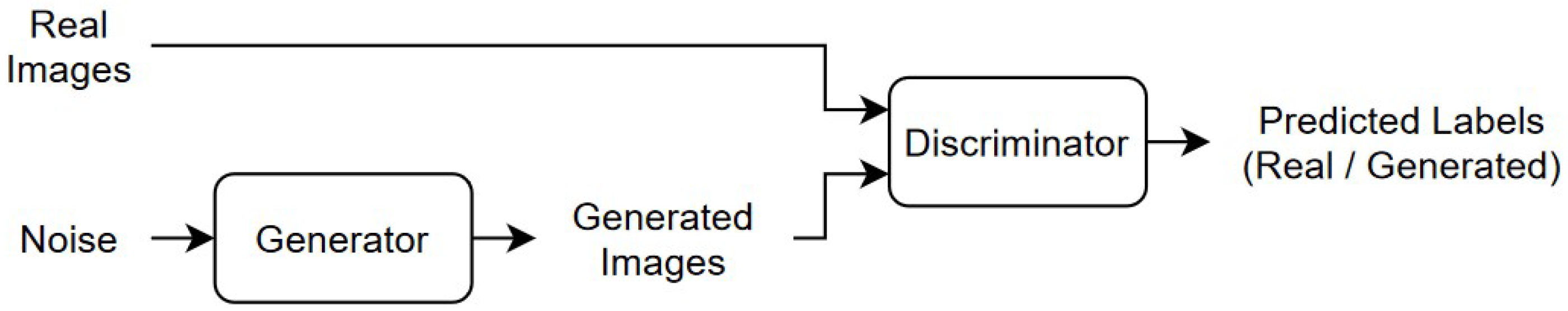
Figure 2.
(L-R & Top-Bottom) (a) RGB image instance (1m) containing a heterogeneous mix of Triticum Aestivum (wheat) and Raphanus Raphanistrum (horseradish). (b) Infrared instance (1m) containing a heterogebous mix of triticum aestivum (wheat) and Raphanus Raphanistrum (horseradish). (c) Clipped samples from (a) at 155 x 115 pixels. (d) Clipped samples from (b) at 155 x 115 pixels.
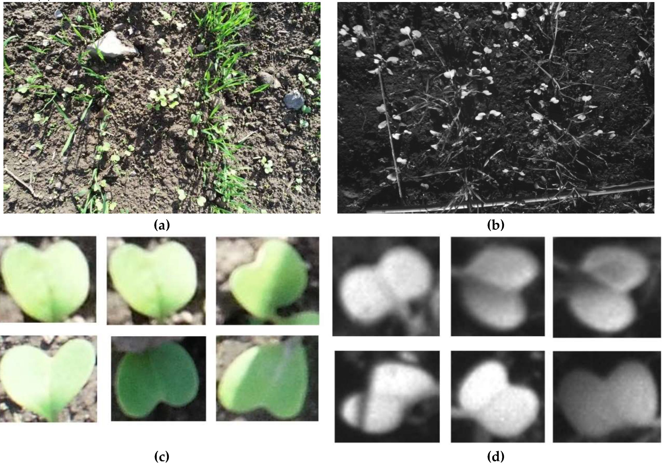
Figure 3.
(a) Training Images (b) Generated Images using WGAN-GP (c) Generated images using modified WGAN-GP.
Figure 3.
(a) Training Images (b) Generated Images using WGAN-GP (c) Generated images using modified WGAN-GP.
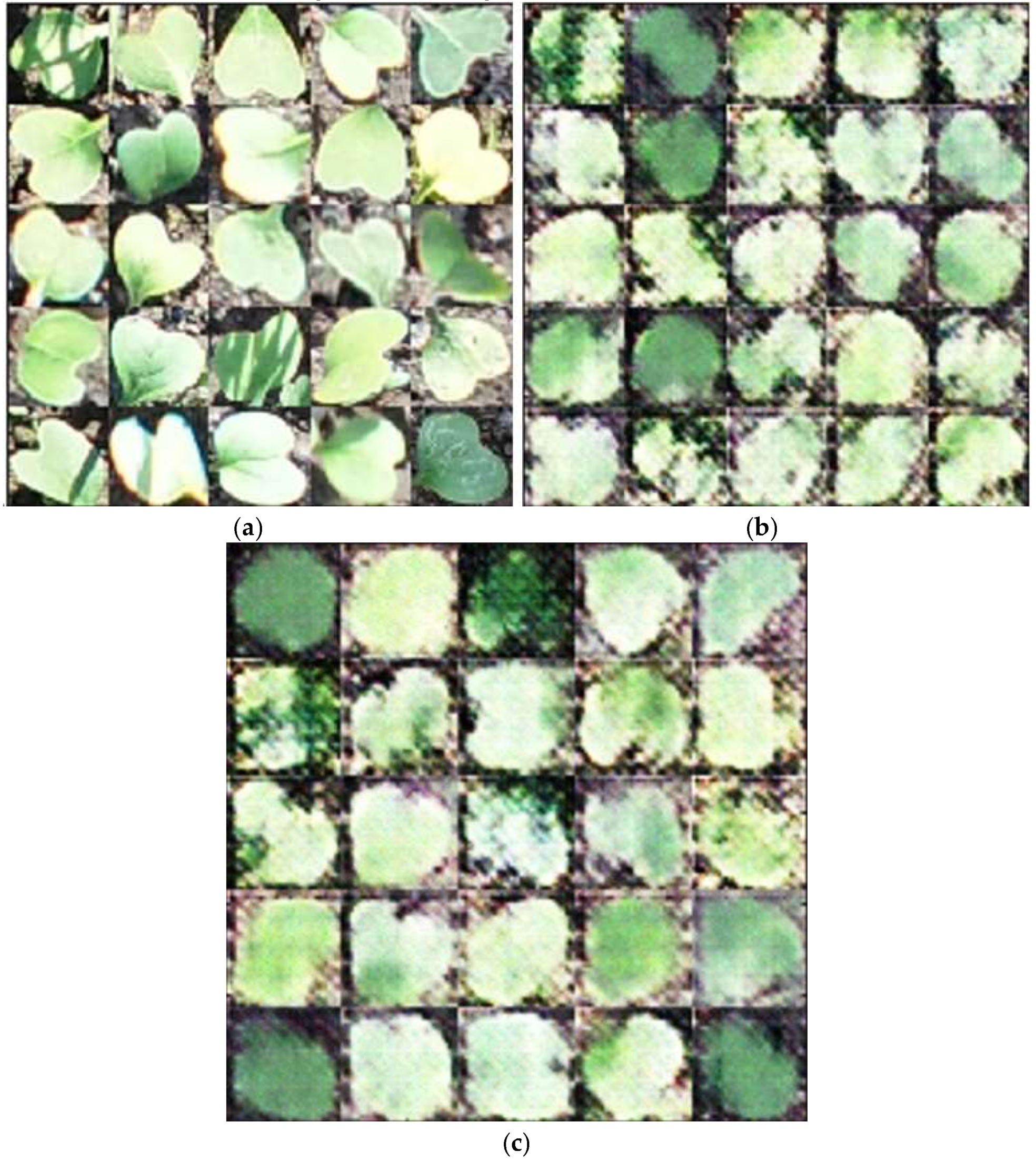
Figure 4.
(a) Training Images (b) Generated Images using WGAN-GP (c) Generated images using modified WGAN-GP.
Figure 4.
(a) Training Images (b) Generated Images using WGAN-GP (c) Generated images using modified WGAN-GP.
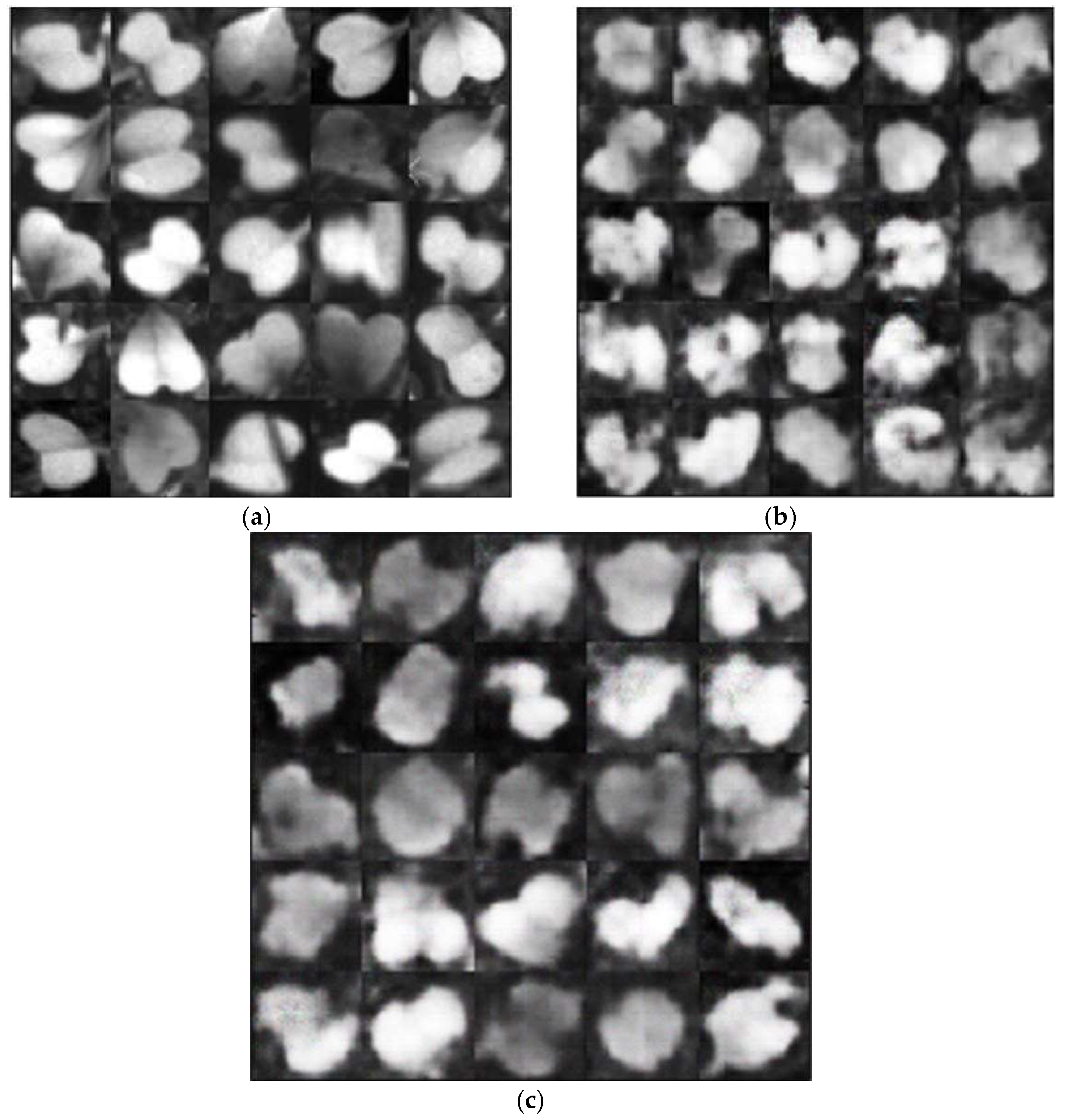
Figure 5.
Comparative analysis of SSIM for different GAN architectures for generated RGB instances.
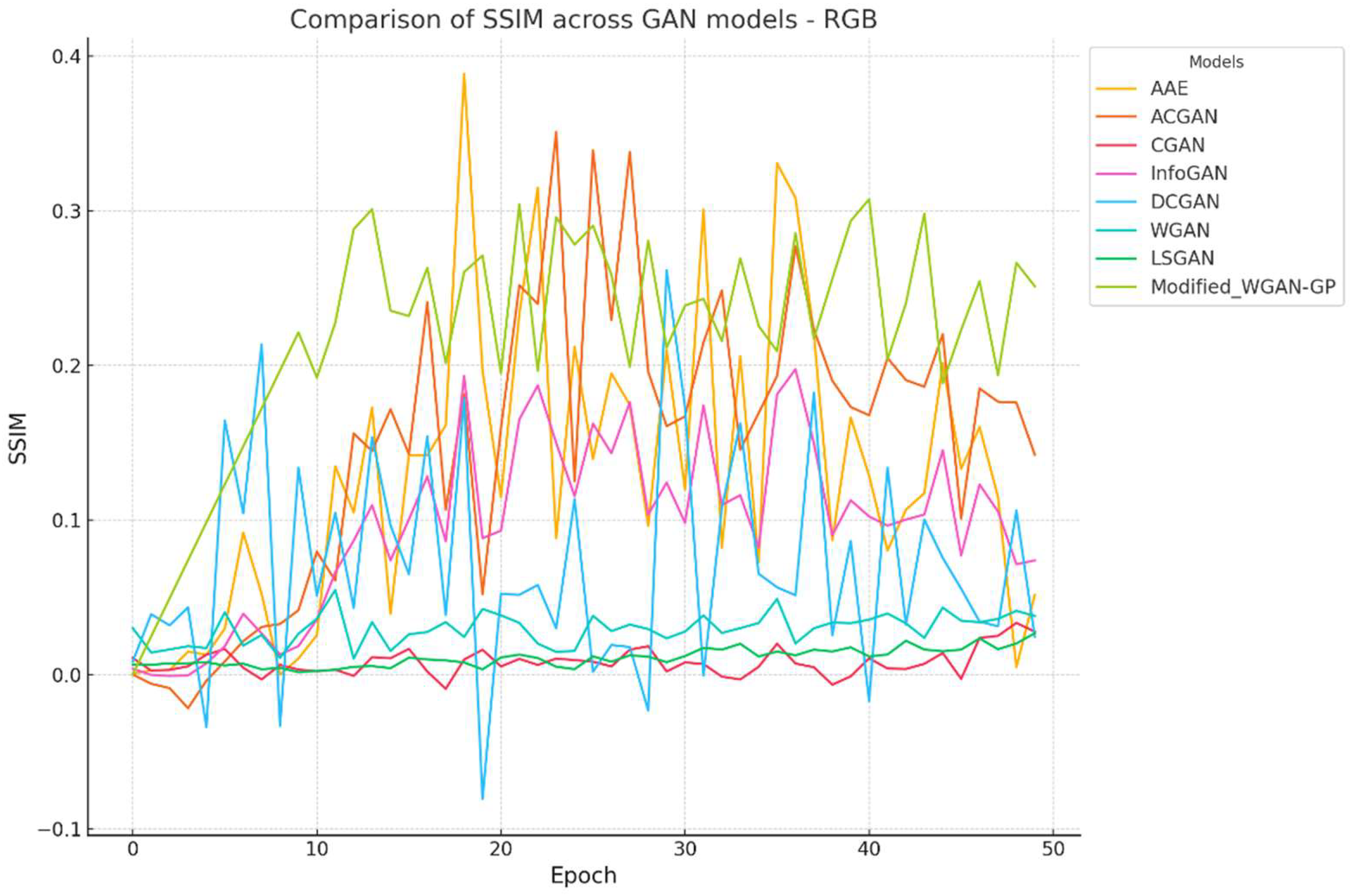
Figure 6.
Comparative analysis of SSIM for different GAN architectures for generated IR instances.
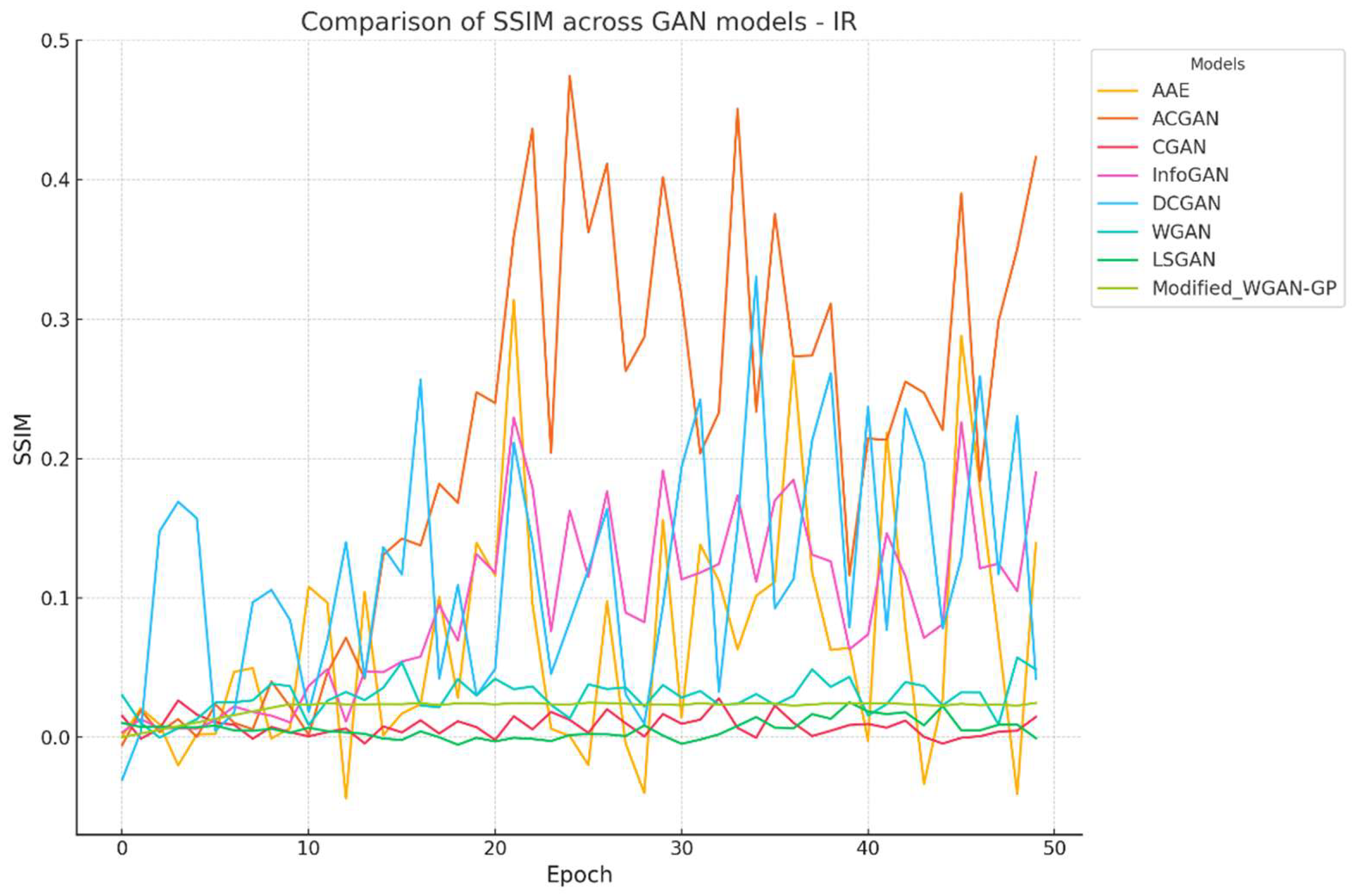
Figure 7.
Raphanus Raphanistrum instances generated by different GAN architectures (a) AAE - RGB (b) AAE – IR (c) CGAN – RGB (d) CGAN – IR (e) CGAN – RGB (f) CGAN – IR (g) DCGAN – RGB (h) DCGAN – IR (i) InfoGAN - RGB (j) InfoGAN – IR (k) WGAN – RGB (l) WGAN – IR (m) LSGAN – RGB (n) LSGAN - IR.
Figure 7.
Raphanus Raphanistrum instances generated by different GAN architectures (a) AAE - RGB (b) AAE – IR (c) CGAN – RGB (d) CGAN – IR (e) CGAN – RGB (f) CGAN – IR (g) DCGAN – RGB (h) DCGAN – IR (i) InfoGAN - RGB (j) InfoGAN – IR (k) WGAN – RGB (l) WGAN – IR (m) LSGAN – RGB (n) LSGAN - IR.
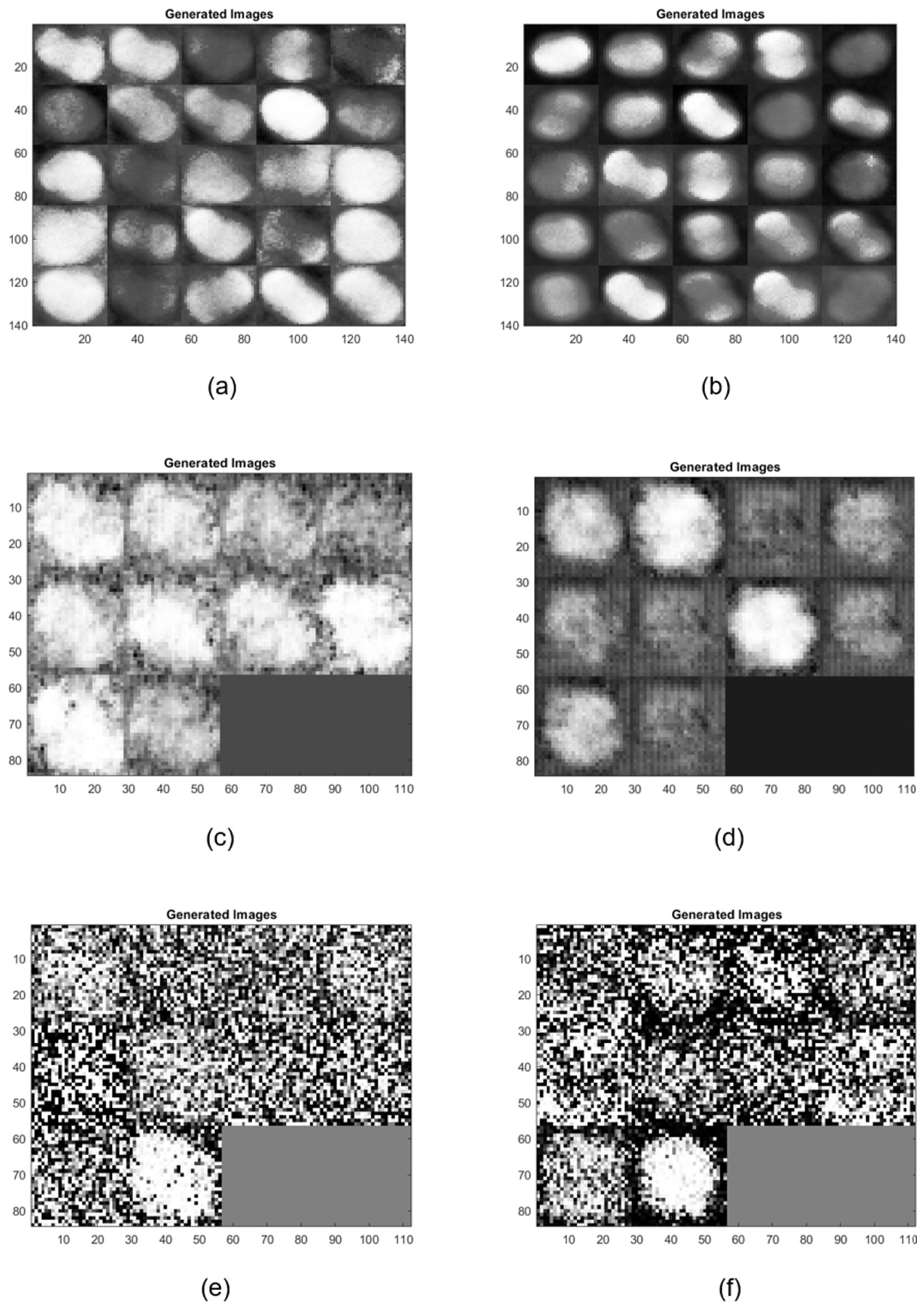
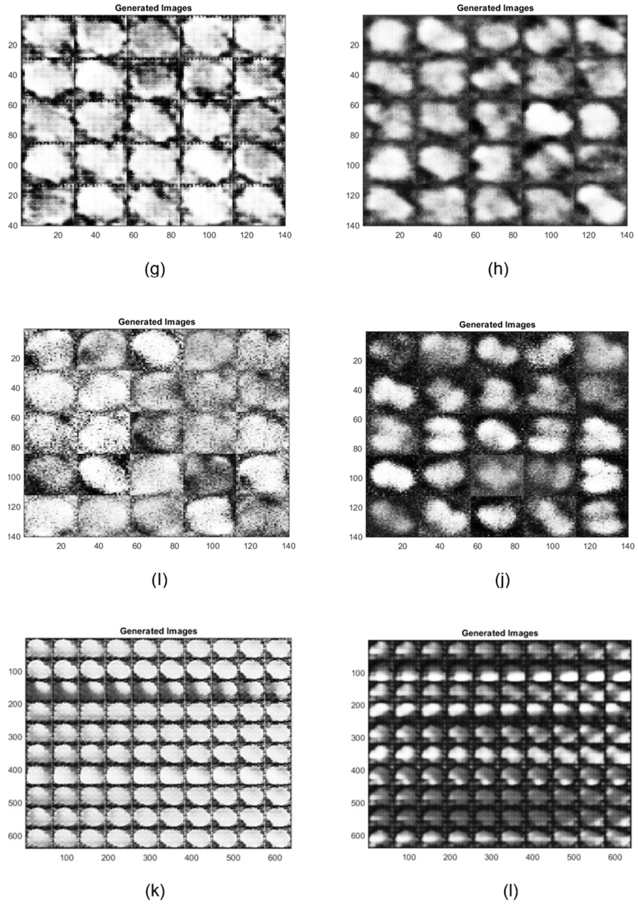
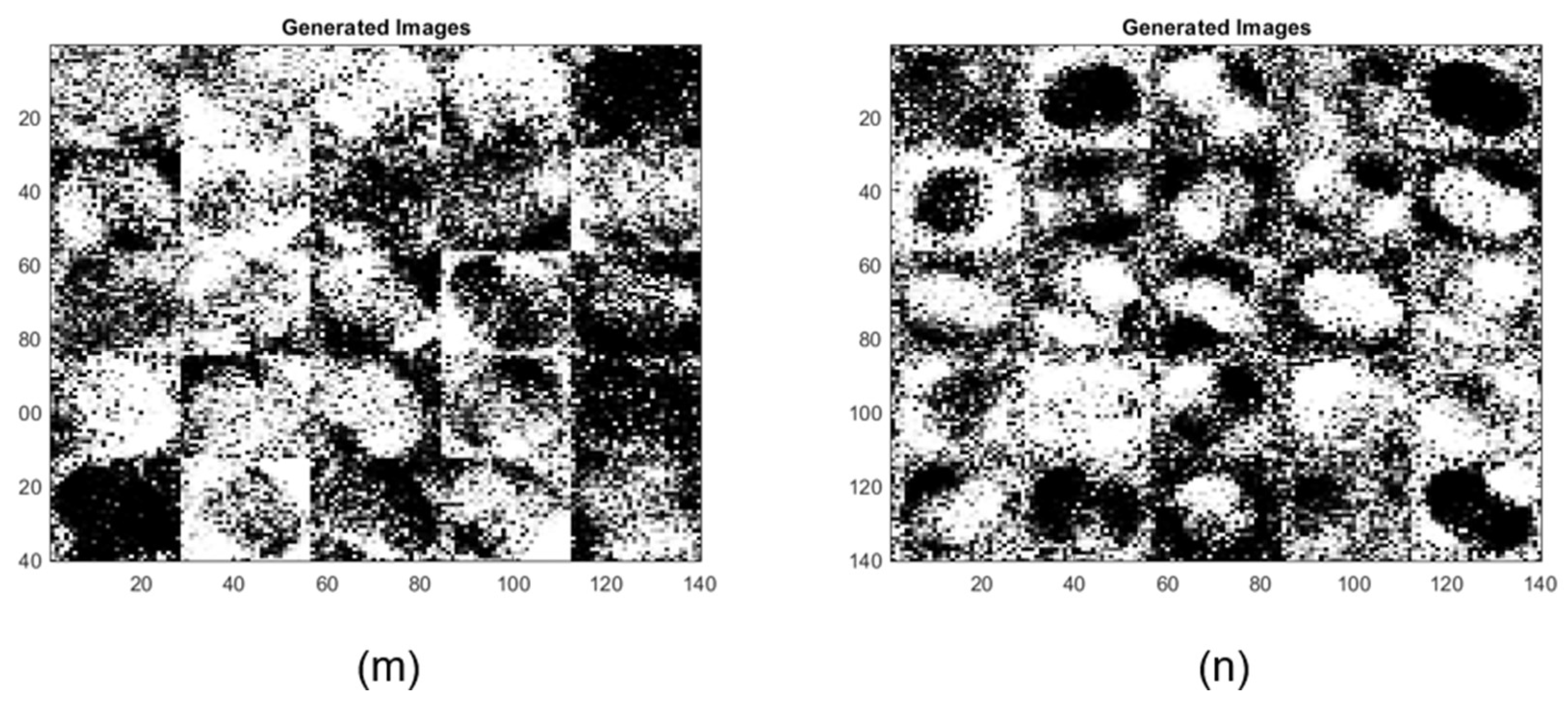

Table 1.
Modified Architecture of WGAN – GP Generator Network.
| Layer | Type | Parameters | Activation Function |
|---|---|---|---|
| 1 | Fully Connected | 128 x 7 x 7 neurons | ReLU |
| 2 | Reshape | 7 x 7 x 128 | - |
| 3 | Transposed Convolution |
4 x 4, 128 filters, stride 2, same padding |
BatchNorm + ReLU |
| 4 | Transposed Convolution |
4 x 4, 64 filters, stride 2, same padding |
BatchNorm + ReLU |
| 5 | Convolution | 4 x 4, 3 filters, same padding | Tanh |
Table 2.
Modified Architecture of WGAN – GP Discriminator Network.
| Layer | Type | Parameters | Activation Function |
|---|---|---|---|
| 1 | Convolution | 3 x 3, 16 filters, stride 2, same padding | Leaky ReLU + Dropout |
| 2 | Convolution | 3 x 3, 32 filters, stride 2, same padding | BatchNorm + Leaky ReLU + Dropout |
| 3 | Convolution | 3 x 3, 64 filters, stride 2, same padding | BatchNorm + Leaky ReLU + Dropout |
| 4 | Convolution | 3 x 3, 128 filters, stride 1, same padding | BatchNorm + Leaky ReLU + Dropout |
| 5 | Fully Connected |
1 neuron |
- |
Disclaimer/Publisher’s Note: The statements, opinions and data contained in all publications are solely those of the individual author(s) and contributor(s) and not of MDPI and/or the editor(s). MDPI and/or the editor(s) disclaim responsibility for any injury to people or property resulting from any ideas, methods, instructions or products referred to in the content. |
© 2025 by the authors. Licensee MDPI, Basel, Switzerland. This article is an open access article distributed under the terms and conditions of the Creative Commons Attribution (CC BY) license (http://creativecommons.org/licenses/by/4.0/).
Copyright: This open access article is published under a Creative Commons CC BY 4.0 license, which permit the free download, distribution, and reuse, provided that the author and preprint are cited in any reuse.


