
Submitted:
07 August 2024
Posted:
08 August 2024
You are already at the latest version
Abstract
High-resolution (2 km) high-frequency (hourly) SST data from 2015-2021 provided by the Advanced Himawari Imager (AHI) onboard the Japanese Himawari-8 geostationary satellite were used to study spatial and temporal variability of the China Coastal Front (CCF) in the South China Sea. The hourly SST data were processed with the Belkin and O’Reilly (2009) algorithm to generate long-term mean monthly maps of SST gradient magnitude (GM) and frontal frequency (FM). The horizontal structure of CCF was investigated from cross-frontal distributions of SST along 11 fixed lines that allowed to determine inshore and offshore boundaries of the CCF and calculate the CCF strength defined as the total cross-frontal step dSST = Offshore SST – Inshore SST. Combined with the results of Part1 of this study (Belkin, Lou, Yin, 2023), where the CCF was documented in the East China Sea, the new results reported in this paper allowed the CCF to be reliably traced from the East China Sea via Taiwan Strait into the northern South China Sea and farther west up to the east coast of Hainan Island.
Keywords:
South China Sea
; Oceanic fronts
; China Coastal Front
; Guangdong Coastal Front
; Taiwan Strait
; Taiwan Bank
; Himawari-8
; Advanced Himawari Imager
1. Introduction
Rationale: The China Coastal Front (CCF) is a major ocean feature in the East China Sea (ESC) and northern South China Sea (NSCS). The CCF is a boundary between coastal waters off the mainland China and offshore waters. The CCF is physically associated and collocated with the China Coastal Current (CCC), which is also called the Zhejiang-Fujian Current or Zhe-Min Current in the ECS and Guangdong Coastal Current throughout the NSCS. Numerous studies of the NSCS elucidated many aspects of its circulation and frontal structure reviewed previously by Su (2004) and recently by Shu et al. (2018). Nonetheless, a detailed, modern climatology of the CCF is missing, probably because most efforts to date were focused on establishing a general frontal pattern of the China Seas before zeroing in on individual fronts. The need to close this knowledge gap was the main incentive for our study of the CCF. In the first part of this investigation, we covered the ECS between 31°N and 24°N (Belkin et al., 2023). The present paper is dedicated to the NSCS between 24°N and 18°N. The Taiwan Strait (TS) is generally considered to be part of NSCS. The northern TS is covered in Part 1 (Belkin et al., 2023), while the southern TS is covered in Part 2 (this paper).
Background: The history of remote sensing studies of oceanic fronts in the NSCS is rather short and is briefly reviewed below. Table 1 sums up relevant studies published in peer-reviewed international English-language journals. A few studies published in Chinese in domestic journals were recently reviewed by Shen and Belkin (2023). The below background is organized chronologically. Regional and thematical aspects are elucidated in subsequent sections of this paper.

Table 1.
Satellite studies of the China Coastal Front in the South China Sea from SST data.
| Reference | Sensor | Period | Algorithm | Region |
|---|---|---|---|---|
| Belkin and Cornillon 2003 | AVHRR | 1985-1996 | CCA1992 | SCS |
| Belkin and Cornillon 2007 | AVHRR | 1985-1996 | CCA1992 | SCS |
| Belkin et al. 2009 | AVHRR | 1985-1996 | CCA1992 | SCS |
| Belkin et al. 2024 (this study) | AHI | 2015-2021 | BOA2009 | NSCS, including TS |
| Chang et al. 2006 | AVHRR | 1996-2005 | S2005 | TS |
| Chang et al. 2008 | AVHRR | 1996-2005 | S2005 | TS (north of 24°N) |
| Chang et al. 2010 | AVHRR | 2001-2007 | S2005 | NSCS, including TS |
| Dong and Zhong 2020 | AVHRR MODIS |
2009-2012 | GM | NSCS, including TS |
| Jing et al. 2015 | OSTIA | 2006-2013 | GM | NSCS |
| Jing et al. 2016 | GHRSST | 2006-2014 | GM | NSCS |
| Lee et al. 2015 | AVHRR | 1996-2009 | S2005 | TS (north of 24°N) |
| Pi and Hu 2010 | Misc.* | 2002-2008 | PH2010 | NSCS, including TS |
| Ping et al. 2016 | MODIS | 2000-2013 | CCA1992 | TS (north of 22°N) |
| Ren et al. 2021 | Model | 2005-2018 | Canny (1986) | SCS |
| Shi et al. 2015 | OSTIA | 2006-2011 | GM | NSCS |
| Wang DX et al. 2001 | AVHRR | 1991-1998 | GM | NSCS, including TS |
| Wang YC et al. 2013 | AVHRR | 2006-2009 | S2005 | TS |
| Wang YC et al. 2018 | AVHRR | 2005-2015 | S2005 | TS (north of 24°N) |
| Wang YT et al. 2020 | MODIS | 2002-2017 | W2020 | NSCS, including TS |
| Xing QW et al. 2023 | AVHRR | 1982-2021 | CCA1992 | China Seas |
| Yu et al. 2019 | MODIS | 2002-2017 | GM | SCS |
| Zeng et al. 2014 | MODIS | 2002-2011 | BOA2009 | East Hainan |
| Zhang L and Dong J 2021 | MODIS | 2016-2017 | GM | NSCS, 250-m L2 data |
| Zhang Y et al. 2021 | OSTIA | 2006-2015 | GM | NSCS, 3D structure |
| Zhao et al. 2022 | DOISST | 1982-2021 | CCA1992 | China Seas |
Place names: SCS, South China Sea; NSCS, Northern SCS; TS, Taiwan Strait. Algorithms and datasets: BOA2009, Belkin and O’Reilly (2009); CCA1992, Cayula and Cornillon (1992); CW2014, Castelao and Wang (2014); PH2010, Pi and Hu (2010); S2005, Shimada et al. (2005); W2020, Wang YT et al. (2020) (combination of Canny (1986), Castelao and Wang (2014), and Wang YT et al. (2015) algorithms); GM, Gradient magnitude; DOISST, Daily Optimum Interpolation SST; OSTIA, Operational SST and Sea Ice Analysis. *) AVHRR, MODIS, and AMSR-E data merged.
After Jean-François Cayula and Peter Cornillon (University of Rhode Island, URI) developed a state-of-the-art edge detection algorithm (based on histogram approach) known as the Cayula-Cornillon algorithm (CCA) and published two seminal papers describing a single-image edge detector (SIED) and multiple-image edge detector (Cayula and Cornillon 1992; Cayula and Cornillon 1995), the CCA was used for a global survey of SST fronts funded by NASA. The main results of this survey (conducted at the University of Rhode Island and based on a 9-km resolution, 11-year Pathfinder dataset, 1985-1996) were presented at the AGU Fall 1998 Meeting by Belkin et al. (1998) and published by Belkin and Cornillon (2003), Belkin and Cornillon (2007), and Belkin et al. (2009).
Meanwhile, back in 2001, Dongxiao Wang and collaborators published a study of SST fronts in the NSCS (Wang et al., 2001), using a 9-km resolution, 8-year Pathfinder dataset (1991-1998, thus overlapping with the URI dataset) and defining SST fronts as pixels with gradient magnitude GM exceeding 0.5°C/9 km. Wang et al. (2001) identified six fronts and determined frontal envelopes (“corridors”) for each front, using a method developed by Hickox et al. (2000) to calculate cross-frontal SST steps across 10 fronts in the East China Seas. Among the six fronts in the NSCS, Wang et al. (2001) identified the Fujian-Guangdong Front and noted that “the coastal fronts off Fujian and Guangdong become a continuous front in wintertime.” (ibid., p. 3966). The maps of long-term mean seasonal frontal probability (frequency) presented by Wang et al. (2001) suggest that the coastal Fujian-Guangdong Front extends westward until ~115°E, where this front abuts another front, the Pearl River (Zhujiang) Estuary coastal front, which in spring protrudes offshore beyond the 50-m isobath. Farther west, beyond the Pearl River front, Wang et al. (2001) identified the Hainan Island East Coast front. Thus, between the Taiwan Strait and East Coast of Hainan, the CCF consists of three disconnected fronts of different origin. This conclusion that seems obvious after a quick inspection of seasonal frontal maps presented by Wang et al. (2001) becomes less obvious in the light of most recent studies discussed below.
Yi Chang and collaborators used the Shimada algorithm (Shimada et al., 2005) to detect and map SST fronts in the NSCS, including the Taiwan Strait (Chang et al., 2006; Chang et al., 2008; Chang et al., 2010; Lee et al., 2015). In a study of winter fronts, Chang et al. (2006) and Chang et al. (2008) used high-resolution (0.01°) data from 1996-2005 to generate long-term monthly mean maps of GM that document the CCF (called the Mainland China Coastal Front, MCCF) and its seasonal variability. The monthly maps of GM presented by Chang et al. (2006), Chang et al. (2008), and Chang et al. (2010) reveal the rather sharp CCF with GM up to 0.3°C/km in January, when the CCF’s intensity peaks. Using 1-km SST data from 2001-2007, Chang et al. (2010) generated maps of frontal frequency FF for December through March. In December and January, the continuous CCF extends along the Fujian-Guangdong coast up to Hainan. During these months, the CCF shows no signs of a local break-up off the Pearl River Estuary. Perhaps, this fact can be explained by the decreased discharge of the Pearl River (Zhujiang) during this season. Indeed, according to the most recent climatology by Liu ZZ et al. (2022, Figure 6) based on the 1954-2020 data, between June and December the Pearl River discharge drops seven-fold from the summer maximum of 50 Gt/month to the winter minimum of ~7 Gt/month. In late winter (February-March), the CCF in the southern Taiwan Strait does not continue along the Fujian-Guangdong coast. Instead, the CCF veers offshore to join the Taiwan Bank Front (TBF). The CCF-TBF merger was noted earlier by Wang DX et al. (2001), Chang et al. (2006), and Chang et al. (2008). Farther west along the Guangdong coast, the CCF shows signs of a breakup off the Pearl River Estuary in spring-summer when the Pearl River discharge sharply increases from ~7 Gt/month in February to ~50 Gt/month in June (Liu ZZ et al., 2022, Figure 6).
The spatial pattern of CCF in the Taiwan Strait remains unclear and inconclusive. For example, the often-repeated claim that the CCF extends along the 50-m isobath is inconsistent with the existence of a broad (~50 km wide) shallow area northwest of the Taiwan Bank, with depths of <40 m and often <30 m (as evidenced by bathymetry maps in Belkin and Lee, 2014, Figure1 and Kuo et al., 2018, Figure 1). This shallow area (submarine isthmus connecting the Bank with the continent) would constrain the CCC and associated CCF. Indeed, surface drifters used by Qiu et al. (2011) mostly avoided this shallow area except for a few drifters that went straight across it. Other drifters went to or around the Taiwan Bank. The existence of two quasi-zonal topographic barriers (Taiwan Bank with the submarine isthmus to the west, and Chang-Yun Rise to the east) gave Huang et al. (2020) a reason to call the Taiwan Strait a “quasi-cul-de-sac” during the winter northeast monsoon.
Shi et al. (2015) used the Operational SST and Sea Ice Analysis (OSTIA) daily data with a spatial resolution of 0.05° from 2006-2011 to calculate monthly mean GM in the NSCS. The monthly maps of GM presented by Shi et al. (2015, Figure 2) reveal the CCF featuring rather low GM (<0.08°C/km), even during winter, when the CCF is best developed. As we are about to see below, such low values of GM obtained in some other studies (e.g., Shi et al., 2022) tend to underestimate the real intensity of the CCF. Nonetheless, even SST fronts of relatively moderate intensity (GM<0.1°C/km) can affect winds in the atmospheric marine boundary layer and therefore be important to marine meteorology and climate (Shi et al., 2015; Shi et al., 2017; Shi et al., 2022).
Shu et al. (2018) reviewed the NSCS circulation and paid special attention to (a) the Guangdong Coastal Current, and (b) the interaction between the Pearl River Plume (PRP) and coastal currents in the NSCS. The PRP-GCC/CCF interaction is highly complicated and variable in time and space owing to a complex interplay of winds, tides, topography, river discharge, stratification, and circulation (e.g., Dong et al., 2004; Zu and Gan, 2015).
Yu et al. (2019) use Level 4 MODIS data with a spatial resolution of 0.04°×0.04° from 2002-2017 to calculate SST gradients (fronts) and SST trends in the SCS. This is probably the first study of long-term variability and trends of SST gradient magnitude (SST GM), which serves as a measure of front intensity or front sharpness, while the front strength is measured by a total SST step (SST range) across the front. Yu et al. (2019, Figure 5a) presented a map of climatological annual mean SST GM that revealed rather small maximum values of GM, just slightly over 0.04°C/km. As mentioned above, such low values underestimate the real maximum values of GM obtained in other studies. For example, using high-resolution (1 km) satellite data from the NSCS shelf, Dong J and Zhong Y (2020) frequently observed sharp SST fronts in winter, with GM exceeding 1.3°C/km. There are at least two factors that might help explain the unrealistically low values of GM reported in some studies: one is the relatively coarse spatial resolution of SST data used in such studies; another is the long-term seasonal or year-round averaging involved in the production of climatic maps of GM. Regarding SST trends, a caveat is that the long-term SST trends in the China Seas tend to abruptly reverse their signs during so-called regime shifts (Belkin and Lee, 2014; Lee et al., 2021). Therefore, caution is needed when such trends are used in research or practice, especially for long-range forecasts.
Wang YT et al. (2020) processed 4.5-km resolution MODIS data from 2002-2017 with their own algorithm that builds on Canny (1986) modified by Castelao and Wang YT (2014) and Wang YT et al. (2015). They used a rather small GM threshold for a front: 1.4°C/100 km or 0.014°C/km. Wang YT et al. (2015, Figure 1b) presented a map of long-term annual mean GM, in which the maximum GM scale value is a mere 0.04°C/km. This rather low maximum scale value of GM is consistent with their previous study (Yu et al., 2019). Also, the maximum scale value of GM can be arbitrarily set to a low value to highlight weak fronts. The seasonal maps of frontal frequency presented by Wang YT et al. (2015, Figure 2) portray the CCF as a robust feature in fall-winter (October-March) but a weak or absent feature in spring-summer (April-September), especially off western Guangdong.
Zhao et al. (2022) used Daily Optimum Interpolation Sea Surface Temperature (DOISST) data from 1982 to 2021 with a spatial resolution 0.25° x 0.25°. The data were processed with the Cayula and Cornillon (1992) single image edge detection algorithm (CCA-SIED) to detect SST fronts in the China Seas and study their spatial and temporal variability on a variety of scales. The CCA-SIED algorithm used is part of the Marine Geospatial Ecology Tools (MGET) developed by Roberts et al. (2010) at Duke University’s Marine Geospatial Ecology Laboratory. Alas, the massive study by Zhao et al. (2022) was hampered by the rather coarse spatial resolution of SST data used.
Summary: The brief review of previous research above reveals a few common threads. First, there was no dedicated studies of the CCF from satellite data, much less a comprehensive seasonal climatology of the CCF. Second, there is a general agreement about the location (path) of the CCF in the NSCS. Third, there is evidence of the CCF’s spatial adjacency to the Taiwan Bank Front. On the negative side, fourth, no physical mechanism was proposed that would physically connect the CCF and Taiwan Bank Front. Fifth, there are strong disagreements (exceeding an order of magnitude) regarding the range (hence maximum values) of SST GM in the SCS.
Objectives and structure of this study: With the above issues in mind, we set out to produce an up-to-date seasonal climatology of the CCF using the most recent satellite SST data of high spatial and temporal resolution. Our reliance on the most recent SST data mitigates possible effects of regional climate change that can be significant when recent data are compared with old data. Our emphasis on high-resolution data is meant to mitigate the detrimental effect of sparse data on gradient estimation. Finally, our approach was two-pronged: (1) elucidate general spatial and temporal patterns of the CCF; (2) provide numerical estimates of monthly SST ranges, maximum GM, and frontal frequency FF as such numerical estimates are required in a variety of academic and applied research and maritime activities.
The structure of this paper is as follows:
2. Data and Methods
We use the same data and methods as in Part 1 of this study focused on the ECS (Belkin et al., 2023). Nonetheless, to make Part 2 (this paper) self-contained, we are providing sufficient descriptions of data and methods similar to the respective section in Part 1 yet abridged.
Himawari-8/9 satellites and Advanced Himawari Imager: The Japanese geostationary meteorological satellites Himawari 8/9 (Bessho et al., 2016) carry the Advanced Himawari Imager (AHI) that has 16 spectral bands (visible light bands #1-3, near-infrared bands #4-6, and infrared bands #7-16), with spatial resolution that varies from 2 km for bands #5-16 to 1 km for bands #1, 2, and 4; and 500 m for band #3. Every 10 minutes the AHI provides full disk images, while cloud-free full disk composite images are available every 4 days. The satellites are stationed at 140.7°E and cover the 80°E-160°W, 60°N-60°S area. In this study, L3 level SST data with 1-hour temporal resolution and 2-km spatial resolution from July 2015 through December 2021 that cover our study area (northern SCS: 18-26°N, 108-122°E) were downloaded from a website operated by the Japan Aerospace Exploration Agency, JAXA (https://www.eorc.jaxa.jp/ptree/). The hourly data are generated by the JAXA from the original 10-minute data. The AHI data are processed with a novel cloud-masking algorithm (which uses 500-m resolution visual images that resolve individual cumulus clouds) and a novel cloud-tracking algorithm; these advanced algorithms combined with high-frequency (every 10 min.) full disk scanning enable the production of cloud-free imagery every four days, which is unprecedented (Bessho et al., 2016).
Front mapping: The Belkin-O’Reilly algorithm (BOA) was used to map SST fronts (Belkin and O’Reilly, 2009). The BOA generates maps of gradient magnitude (GM) and gradient direction (GD). Frontal maps are generated by setting a threshold T for GM. Every pixel with GM>T is considered a frontal pixel. Once frontal maps are generated, maps of frontal frequency FF over any time period are generated. Pixel-based FF is calculated as a ratio FF=NF/CloudFree, where NF is the total number of times the given pixel was frontal, and CloudFree is the total number of times the given pixel was cloud-free. Gradient magnitude GM is a metric of front’s sharpness (or intensity), while frontal frequency FF is a metric of front’s stability (or robustness).
Front strength and cross-frontal ranges of oceanic variables: Another important aspect of every front is its strength defined as the total cross-frontal range (or cross-frontal step or change) of the oceanic variable in question. In satellite oceanography, Hickox et al. (2000) pioneered a rigorous approach to systematically estimate cross-frontal ranges by defining frontal boundaries and frontal envelopes (“corridors”) using maps of frontal frequency. In the most recent study, Belkin et al. (2023) used a different method by analyzing distributions of SST along a series of closely spaced cross-frontal sections. This approach allows both cross-frontal and along-frontal variability to be visualized. Here we extended this approach from the ECS into the NSCS.
Downstream tracking of CCF: To investigate the CCF extension from the ECS into the NSCS, we used a simple but efficient technique of downstream tracking of ocean fronts. This approach was developed by Belkin and Gordon (1996) in their study of the Southern Ocean fronts. Later, Belkin et al. (2002) used this approach to trace the Polar Front across the North Pacific. Most recently, this approach was used by Belkin et al. (2023) to study the CCF in the ECS. The central idea of downstream tracking can be formulated as follows: (1) make a provisional map of a front in question; (2) find a large number of cross-frontal oceanographic sections and arrange them along the front to minimize section-to-section spacing; (3) along each cross-frontal section, determine frontal parameters (e.g., SST) on both sides of the front; (4) visualize and analyze downstream distribution of frontal parameters.
3. Results
3.1. Introduction
In this section we present the most important results, namely long-term mean monthly maps of SST, GM, and FF, and plots of SST along cross-frontal sections. These maps and plots visualize key frontal parameters: (1) intensity identified with gradient magnitude GM, (2) robustness quantified as pixel-based frontal frequency FF, and (3) strength measured as the total cross-frontal range of SST.
The Supplementary Materials include a collection (“atlas”) of frontal maps that consists of (1) individual monthly maps of gradient magnitude GM and frontal frequency FF, covering the study period from August 2015 through December 2021, (2) long-term mean monthly maps of GM and FF, and (3) long-term mean annual maps of GM and FF. The Supplementary Materials also include plots of monthly SST versus distance along 11 fixed lines (7 meridians and 4 parallels) across the northern SCS.
3.2. Sea Surface Temperature
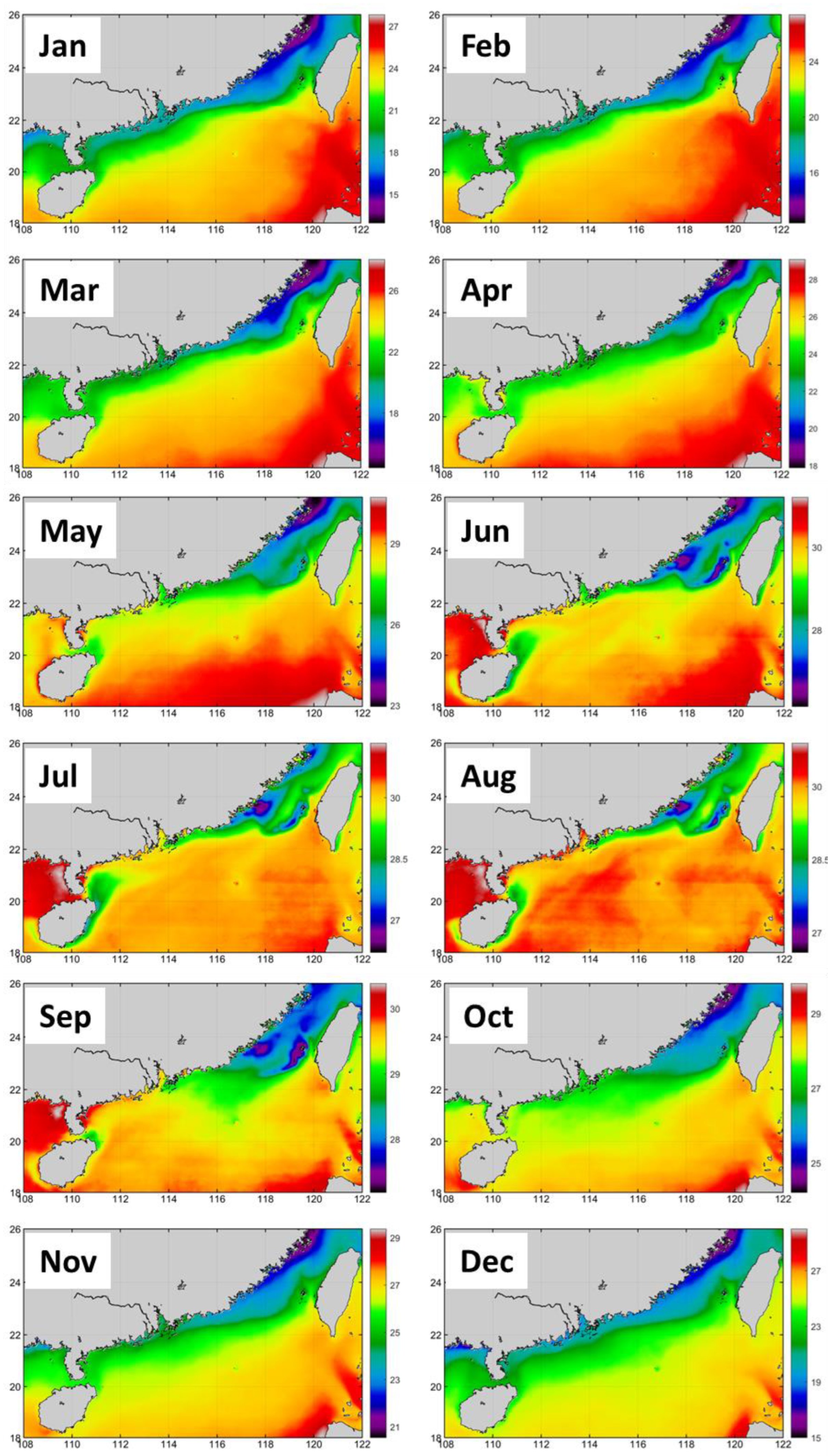
The long-term (2015-2021) mean monthly maps of SST (Figure 1) visualize seasonal evolution and spatial variability of surface temperature in the northern SCS. Overall, the large-scale pattern of SST in the northern SCS (NSCS) has two distinct seasons – winter (November through April) and summer (May-October) – in accordance with the monsoon-driven climate of this region.
3.2.1. Winter
After a summer-to-winter transition in October, the winter pattern of SST in the NSCS is established in November and persists through April (Figure 1). This pattern can be exemplified by the month of January, when the coastal waters are relatively uniform along the entire Guangdong Coast between the Taiwan Strait in the east and Leizhou Peninsula/Qiongzhou Strait in the west. Across this 700-km distance, the coastal SST varies very little in the alongshore direction, remaining within a mere two-degree range between 17-19°C. The cross-shelf gradient of SST is also uniform in the alongshore direction. The shelf-break is roughly demarcated by the 23°C isotherm along the entire northern shelf of the SCS. Thus, across the shelf, the SST varies between 17-23°C in the east (near Taiwan Strait) and 19-23°C in the West (near Hainan). The alongshore uniformity of SST is suggestive of the dominant role of alongshore advection by the Guangdong Coastal Current. This explanation is consistent with the winter wind-driven circulation pattern forced by winter monsoon-associated northeasterlies. The tongue of cold near-shore waters (15-17°C) along the Fujian Coast manifests the China Coastal Current (Zhe-Min Current), which flows south, being driven by winter monsoon’s northeasterlies.
3.2.2. Summer
After a winter-to-summer transition in May, the summer pattern of SST in the NSCS is established in June and persists essentially unchanged through September (Figure 1). The summer pattern features upwellings in two areas: Taiwan Strait and east of Hainan Island. The Taiwan Strait upwelling consists of two centers: one over the Taiwan Bank, another off the Fujian Coast. Both centers remain quite robust over a 4-month period in June-September. Compared with the Taiwan Bank upwelling, the East Hainan upwelling is relatively short-lived, being best developed over a 2-month period in June-July, significantly weakened in August, and almost completely disappeared in September. During summer, the coastal waters off the Guangdong Coast cannot be reliably distinguished from SST maps alone as the summertime warming reduces horizontal gradients of SST. As a result, the entire shelf of the NSCS is covered with uniformly warm waters (29-30°C). Neither the CCF nor the shelf-slope front south of the Guangdong Shelf can be identified from the summertime SST maps.
Figure 1.
Long-term (2015-2021) mean monthly SST (°C) in the northern South China Sea.Color scales are adjusted monthly according to the respective monthly ranges of SST.
Figure 1.
Long-term (2015-2021) mean monthly SST (°C) in the northern South China Sea.Color scales are adjusted monthly according to the respective monthly ranges of SST.
3.2. SST Gradient Magnitude GM
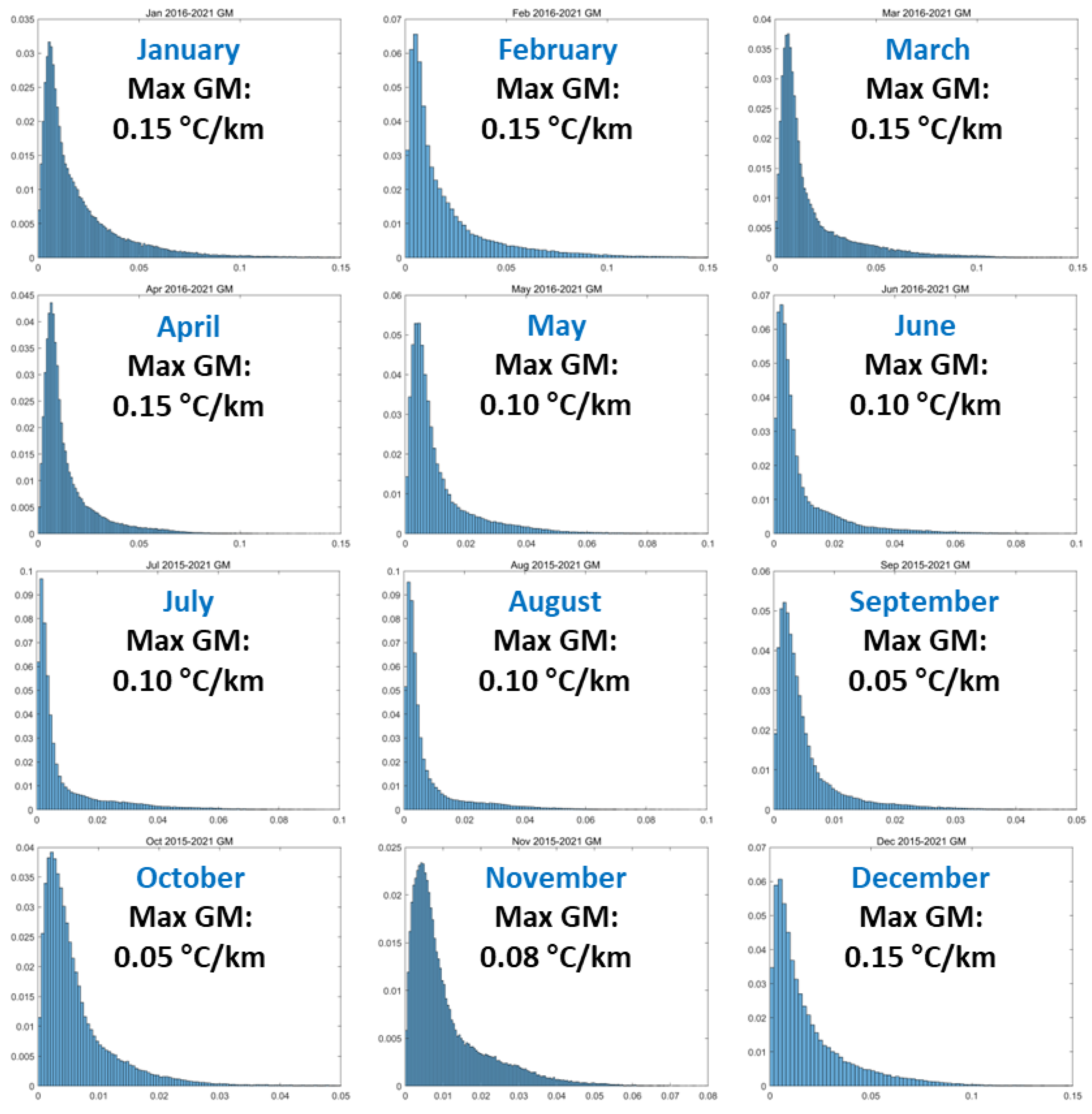
Horizontal gradients of SST are typically at maximum in winter and at minimum in summer, when summertime warming all but obliterates surface manifestations of most fronts (e.g., Hickox et al., 2000). Therefore, to elucidate spatial patterns of horizontal gradients of SST (thermal fronts) and their seasonal variability, Belkin et al. (2023) used dynamic scaling of SST gradient magnitude GM. Specifically, monthly maps of GM were generated by adjusting color scales for GM based on monthly ranges of GM determined statistically from monthly histograms of GM (Figure 2). These histograms reveal maximum values of GM in winter (up to 0.15°C/km), while summertime GM are much smaller and do not exceed 0.05°C/km in September-October.
Figure 2.
Histograms of long-term (2015-2021) mean monthly SST gradient magnitude GM.
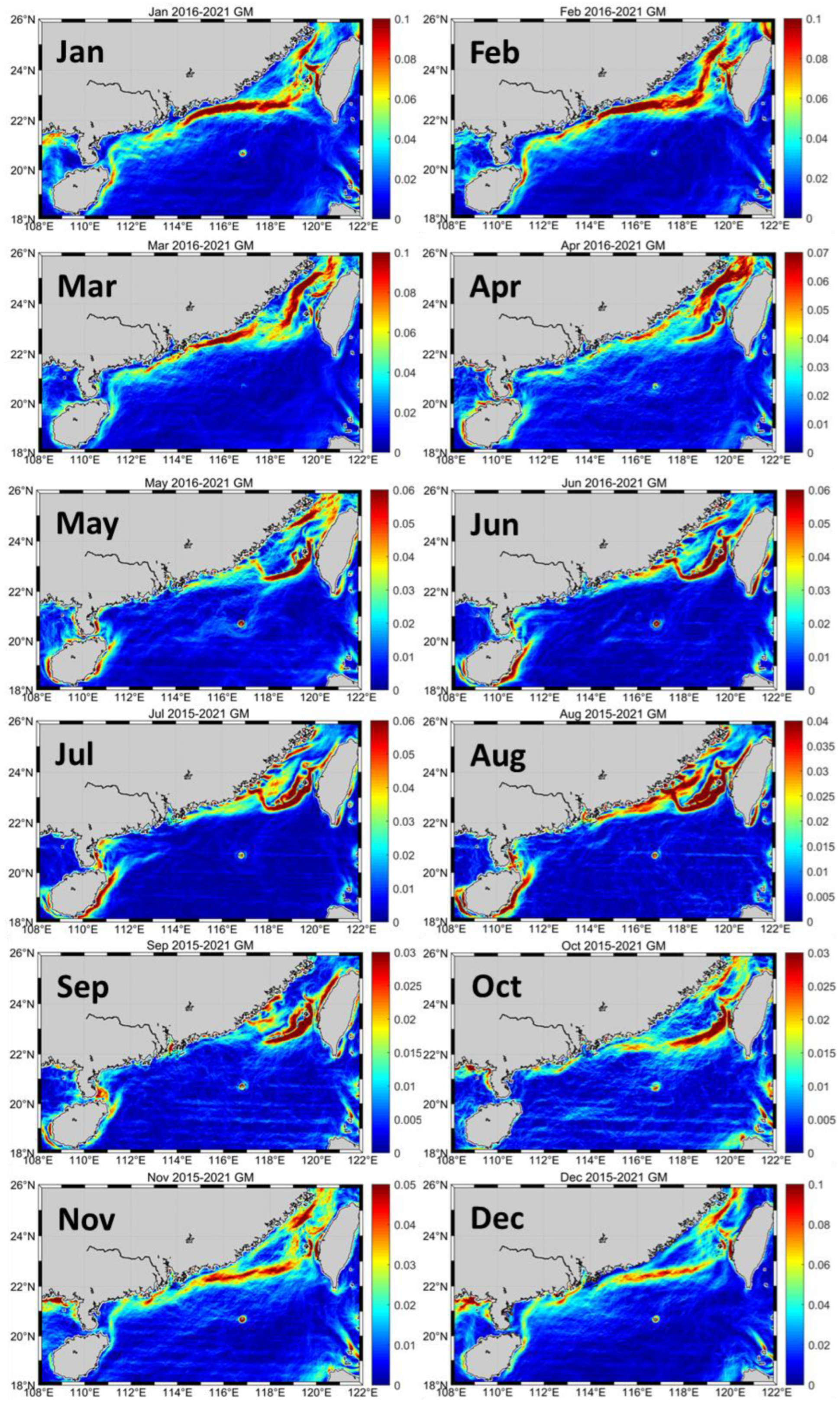
The long-term mean monthly maps of SST gradient magnitude GM (Figure 3) reveal high-gradient zones (fronts) and their spatial and temporal variability. The most striking feature of the temporal variability is dramatic changes of the frontal pattern on the monthly time scale. In that respect, the northern SCS differs from the ECS, where the frontal pattern evolves on the seasonal time scale (Belkin et al., 2023).
Figure 3.
Long-term (2015-2021) mean monthly gradient magnitude GM of SST. Color scales of GM are adjusted monthly using the respective monthly histograms of GM (Figure 2). .
Figure 3.
Long-term (2015-2021) mean monthly gradient magnitude GM of SST. Color scales of GM are adjusted monthly using the respective monthly histograms of GM (Figure 2). .
3.3. Statistics of SST Fronts: Frontal Frequency Maps
Figure 4.
Long-term (2015-2021) mean monthly frontal frequency FF at GM≥0.1°C/km.
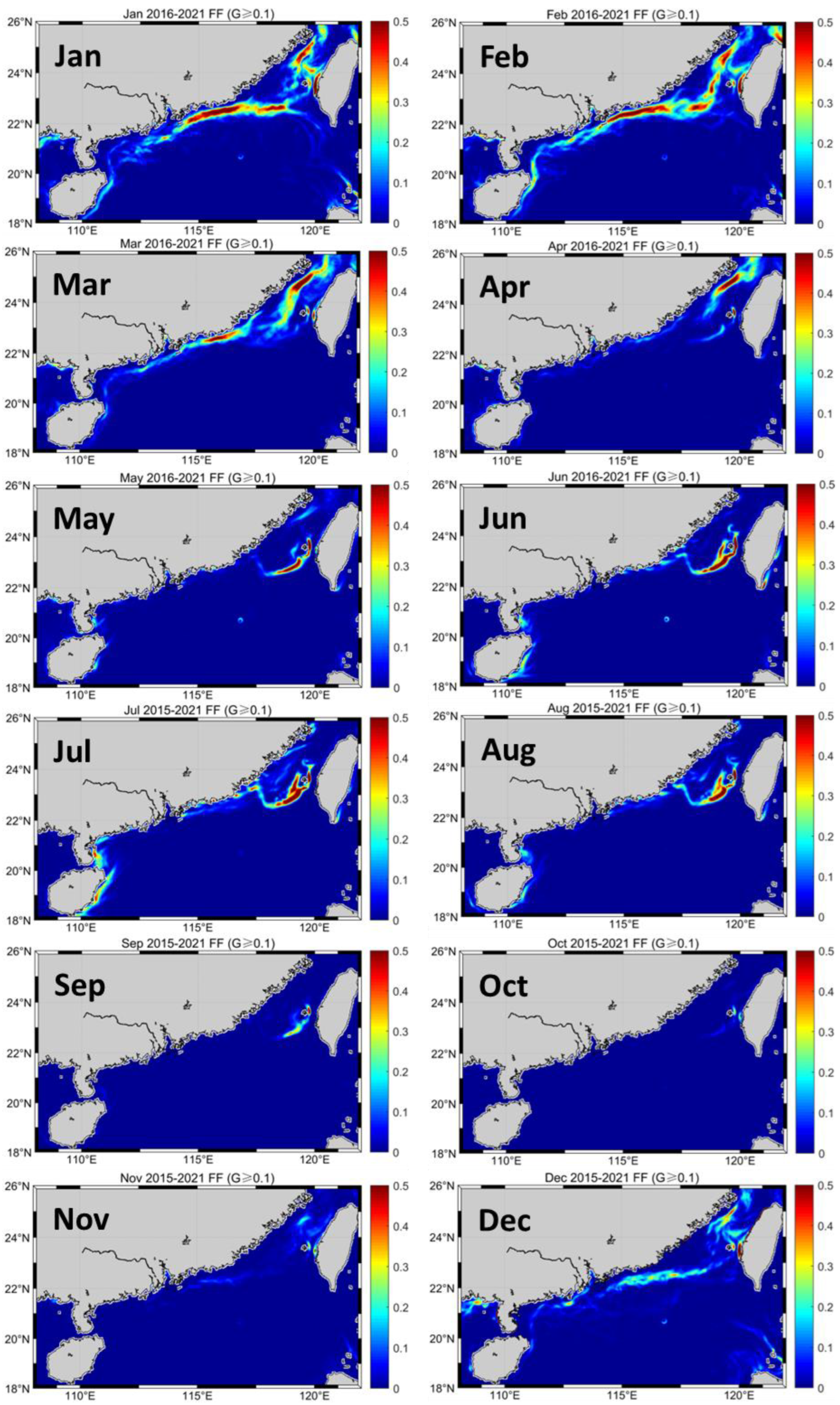
Pixel-based FF in Figure 4 is calculated as the number of times the given pixel’s GM exceeded the threshold of 0.1°C/km divided by the total number of observations during the given month. The large-scale patterns of fronts in FF maps (Figure 4) and GM maps (Figure 3) are mutually consistent. The main difference between the two is that the FF maps bring out the most robust (stable) fronts that retain their location during the given time period (month, year etc.). At the same time, inevitably, the FF maps leave out myriads of migrating mesoscale and submesoscale fronts that do not show up in the FF maps. Such dynamic small-scale fronts may play a significant role in marine ecology owing to their ubiquity and sheer numbers. Statistics and ecological role of such dynamic small-scale fronts remain unexplored. Any statistical metrics of such fronts should include integration over a study area as opposed to pixel-based statistics. An example of such integral metrics (frontal index F1) is provided by Belkin and Cornillon (2005) in their study of the Bering Sea SST fronts from satellite data.
3.4. Cross-Frontal Distributions of SST along Fixed Lines across the Northern SCS
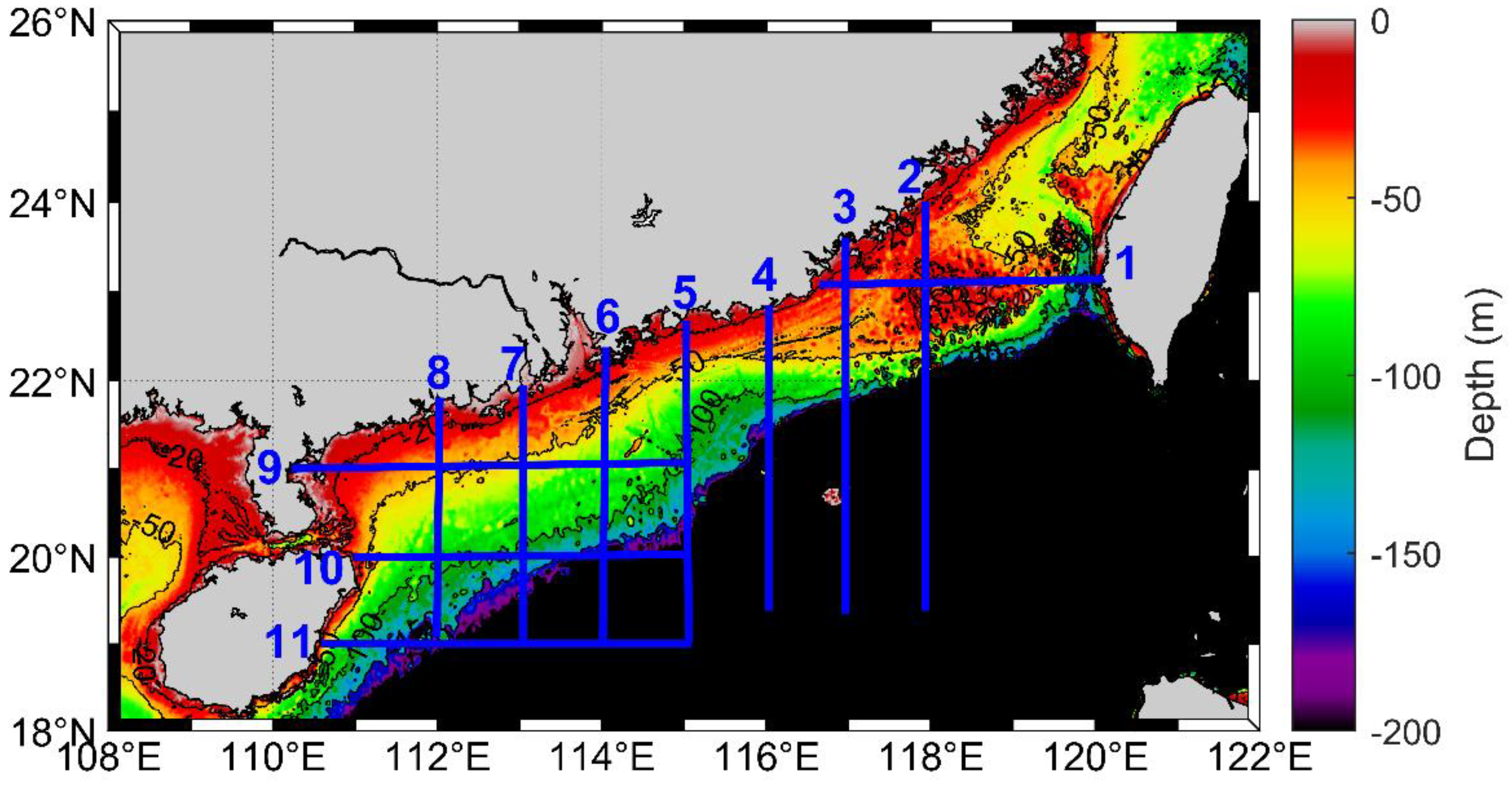
To explore the cross-frontal structure of SST, we plotted long-term mean monthly SST along 11 fixed lines across the northern SCS, including 4 parallels (23°N, 21°N, 20°N, 19°N) and 7 meridians between 112°E and 118°E (Figure 5).
Figure 5.
Bathymetry of the northern South China Sea and locations of 11 fixed lines.
The waterfall plots of SST along the 11 fixed lines (Figure 6 and Figure 7) reveal mesoscale and submesoscale details of the cross-frontal structure of the SST field that are not apparent in maps of SST (Figure 1), GM (Figure 3), and FF (Figure 4). The waterfall plots of SST vs. offshore distance also allow accurate estimation of cross-frontal SST steps dSST defined as offshore SST minus inshore SST. The accurate estimation of dSST depends on the accurate demarcation of the offshore and inshore boundaries of the front in question. For more methodological details see Part 1 of this study by Belkin et al. (2023).
Figure 6.
Long-term (2015-2021) mean monthly distributions of SST along 11 meridional and zonal lines across the northern South China Sea during winter months (November through April). The SST curve numbers in plot legends correspond to the fixed line numbers in Figure 5.
Figure 6.
Long-term (2015-2021) mean monthly distributions of SST along 11 meridional and zonal lines across the northern South China Sea during winter months (November through April). The SST curve numbers in plot legends correspond to the fixed line numbers in Figure 5.
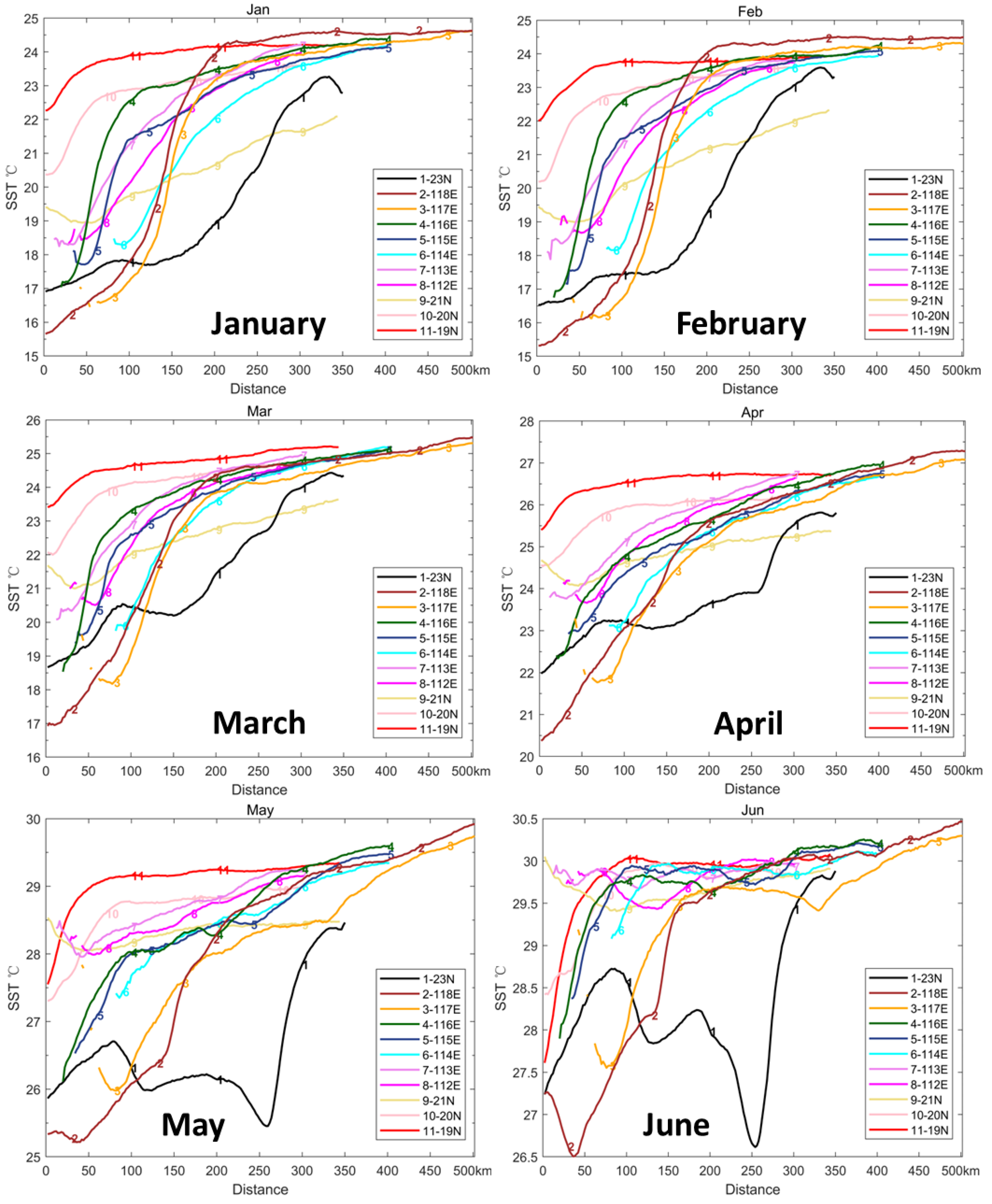
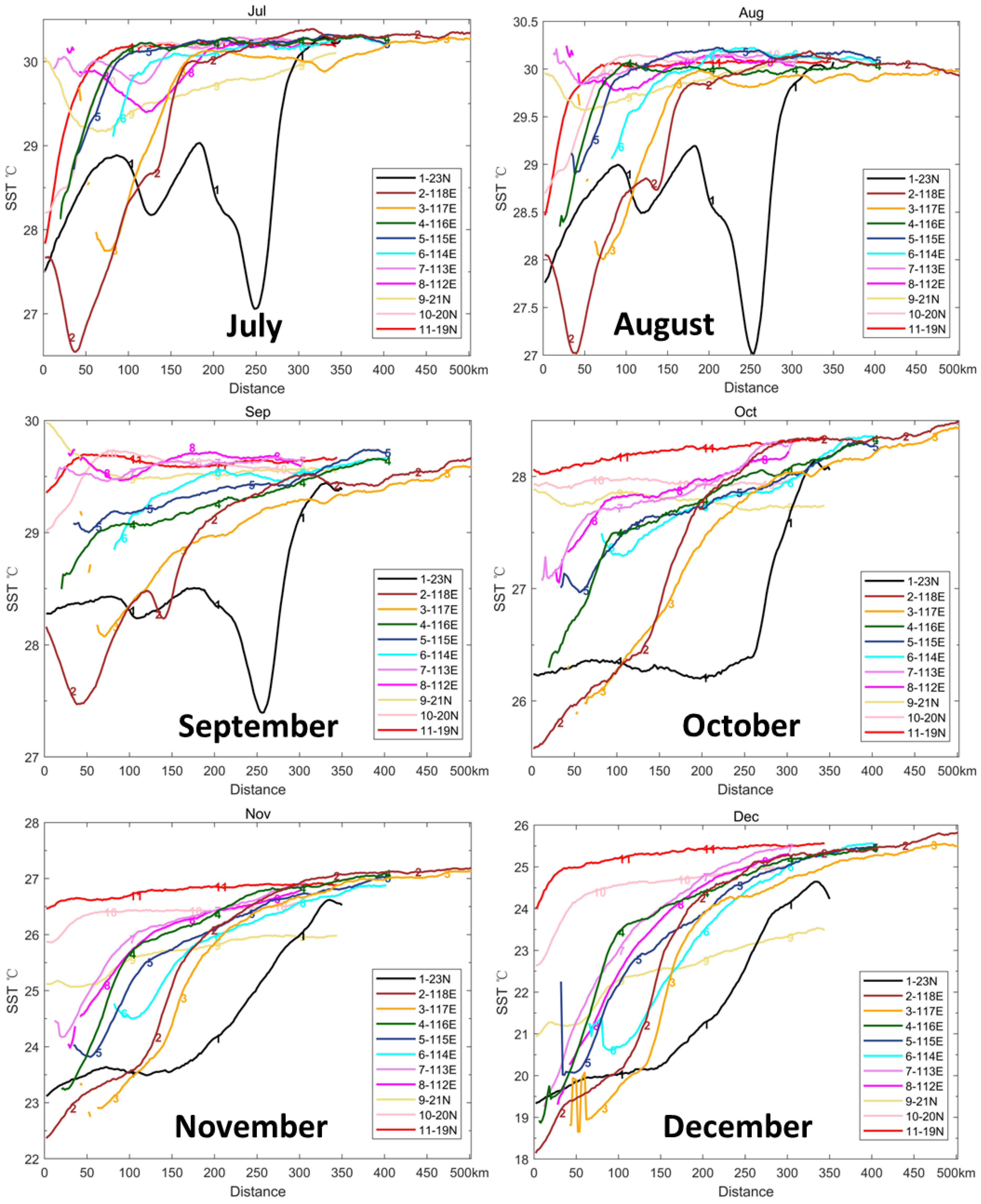
Figure 7.
Long-term (2015-2021) mean monthly distributions of SST along 11 meridional and zonal lines across the northern South China Sea during summer months (May through October). The SST curve numbers in plot legends correspond to the fixed line numbers in Figure 5.
Figure 7.
Long-term (2015-2021) mean monthly distributions of SST along 11 meridional and zonal lines across the northern South China Sea during summer months (May through October). The SST curve numbers in plot legends correspond to the fixed line numbers in Figure 5.
3.5. Analysis of SST Distributions along 11 Fixed Lines across the Northern SCS
The monthly waterfall plots of SST (Figure 6 and Figure 7) allow identification and accurate estimation of various fronts in the NSCS. Even though this study is squarely focused on the CCF, we also consider a few other fronts adjacent to the CCF, namely the Taiwan Bank upwelling front, Fujian upwelling front, East Hainan upwelling front, Taiwan Warm Current front, and Pearl River plume front.
China Coastal Front (CCF): This front develops in winter (November-April) when it stands out in SST plots along 8 fixed lines (Nos. 1-8) yet tapers off between Line 8 and Line 9 (Figure 6). During November through February/March, cross-frontal distributions of SST are remarkably similar between 118°E and 112°E. This qualitative similarity is suggestive of strong alongshore advection by the Guangdong Coastal Current. Quantitatively, cross-frontal ranges of SST decrease downstream (westward) along the front between 118°E and 112°E yet remain substantial even at 112°E, especially in mid-winter (Table 1).
Table 1.
SST ranges (°C) across the CCF in the northern SCS determined from wintertime SST distributions along Lines 1-11 (Figure 6). The locations of Lines 1-11 are shown over bathymetry in Figure 5. Note: Lines 1 and 2 in the two rightmost columns are swapped since Line 2 crosses the CCF upstream of Line 1 (as evident from a detailed analysis of all data). Now all lines (columns) are arranged along the CCF, going downstream from right to left, with Lines 1-8 arranged east to west and Lines 9-11 arranged north to south (Figure 5). Asterisks mark unreliable values when the front’s boundary is poorly defined. Exclamation signs mark the most reliable values associated with well-defined boundaries of the front.
| Line No. | 11 | 10 | 9 | 8 | 7 | 6 | 5 | 4 | 3 | 1 | 2 |
|---|---|---|---|---|---|---|---|---|---|---|---|
| Lon/Lat | 19N | 20N | 21N | 112E | 113E | 114E | 115E | 116E | 117E | 23N | 118E |
| Nov | 26.5-26.7* | 25.9-26.4 | 25.1-26.0 | 24.0-26.0 | 24.2-26.0 | 24.5-25.8 | 23.8-25.5 | 23.2-25.8 | 22.8-27.0 | 23.6-26.7 | 22.4-27.2 |
| Dec | 24.0-25.0 | 22.6-24.7 | 21.2-23.5* | 20.3-25.3* | 19.6-25.5* | 20.6-25.7* | 20.1-22.9* | 19.7-23.7 | 20.2-24.3 | 20.1-24.7 | 18.2-25.1 |
| Jan | 22.3-23.8* | 20.4-22.9 | 19.0-22.0* | 18.5-24.0* | 18.3-24.2* | 18.3-24.2* | 17.7-21.4! | 17.2-23.0! | 16.5- 24.2* |
17.7-23.3! | 15.7-24.3! |
| Feb | 22.0-23.7 | 20.2-22.8* | 19.0-22.2* | 18.7-23.7* | 18.4-23.8* | 18.2-24.0* | 17.5-21.5 | 16.8-22.7* | 16.2-23.7 | 17.5-23.6 | 15.3-24.3 |
| Mar | 23.5-24.5 | 22.0-24.2 | 21.0-23.6* | 20.5-24.5* | 20.3-24.9* | 19.9-25.3* | 19.6-22.3 | 18.5-23.4* | 18.2-23.8 | 20.2-24.5 | 17.0-24.6 |
| Apr | 25.4-26.4* | 24.5-26.0 | 24.1-25.3* | 23.6-26.6* | 23.7-26.7* | 23.1-26.7* | 23.0-26.7* | 22.3-27.0 | 21.8-27.1* | 23.9*-25.8 | 20.4-25.7 |
Comments on Table 1: The CCF is prominent in winter between 118E and 112E, that is between the Taiwan Strait and the vicinity of Leizhou Peninsula. The cross-frontal SST range (offshore SST minus inshore SST) is at maximum in the middle of winter in the Taiwan Strait, with the absolute maximum of 9.0°C (February, 118°E). Moving downstream (westward), the cross-frontal SST range decreases from between 6 and 8°C in the east down to between 5 and 6°C in the west. These rather high values are for mid-winter only (largely January and February). The respective values for transition months (early winter and late winter) are smaller yet significant, varying from 5°C in the east down to between 2°C and 3°C in the west. Overall, the monthly wintertime SST ranges across the CCF in the NSCS are higher than those in the ECS, the latter determined by Belkin et al. (2023) from the same data in Part 1 of this study. This result may appear to be somewhat counter-intuitive because the SST gradient magnitude GM values in the ECS are much higher than those in the NSCS, 0.3-0.4°C/km vs. 0.15°C, respectively, according to Belkin et al. (2023). These results can be summed up as follows: The CCF in the NSCS is less intense (less sharp) but stronger than the CCF in the ECS. The lesser intensity of the CCF in the NSCS is explained by the front being much wider in the NSCS than in the ECS.
Western terminus of the CCF in the NSCS: The CCF tapers off between Line 8 along 112°E and Line 9 along 21°N (Table 1). The front’s abrupt weakening over such a short distance is remarkable. Indeed, in winter the CCF is well-defined along Line 8 but poorly defined along Line 9 (Table 1). Farther south, off Hainan’s eastern coast, Line 10 (20°N) and Line 11 (19°N) crossed a narrow coastal front with a mid-winter cross-frontal SST range of up to 2.5°C. Is this front the real terminus of the CCF? A provisional answer is no because the coastal front off eastern Hainan is very narrow compared with the very wide CCF in the NSCS as evidenced by cross-frontal distributions of SST in winter (Figure 6). Also, the CCF is linked to the westward Guangdong Coastal Current, which extends to the Gulf of Tonkin (Bakbo Bay or Beibu Gulf) via the Qiongzhou Strait (Hainan Strait) between the Leizhou Peninsula and Hainan (Shi MC et al., 2002; Lao et al., 2022). Is there any evidence of the Guangdong Coastal Current branching south before entering the Qiongzhou Strait to flow west? Yes, available evidence supports this view. According to schematics by Lao et al. (2022), the West Guangdong Coastal Current bifurcates while approaching the Qiongzhou Strait, with the southward branch flowing past the North Cape of Hainan Island. Thus, the southward extension of the Guangdong Coastal Current could be linked to the southward terminus of the CCF off eastern Hainan, especially in winter. The southward advection from the West Guangdong Shelf is invoked by Li JY et al. (2023) to explain Chl-a variations off the east coast of Hainan Island.
East Hainan front: This front persists year-round except October, which appears as a transition month between summer and winter seasons (Figure 6, Figure 7, and Table 2). In summer, this front is maintained by wind-driven coastal upwelling generated by the monsoon-related southwesterlies (e.g., Jing ZY et al., 2015; Jing ZY et al., 2016). The strength of the front (identified with the total SST range across the front) in summer exceeds 2°C, peaking at 2.4°C in June-July along Line 11 at 19°N (Table 2). In winter, this front’s dynamics is different since the front is largely maintained by the southward advection from the north. The strength of the front in winter peaks at 2.5°C in February along Line 10 at 20°N, thus rivaling the maximum strength of this front in summer (Table 2).
Taiwan Strait upwelling fronts: During the summer season (May-October), the persistent upwelling-favorable southwesterlies result in the formation of upwelling fronts in the Taiwan Strait. The upwelling fronts can be easily recognized in cross-frontal distributions of SST by their signature V-shape as illustrated and discussed in Part 1 of this study by Belkin et al. (2023). The seasonal development of the upwelling front east of the Taiwan Bank is well documented by monthly distributions of SST along Line 1 at 23°N (Figure 7). The Taiwan Bank upwelling front emerges in May and is fully developed from June through September (Figure 7 and Table 3). West of this upwelling, the SST distribution along 23°N (Line 1) has a distinct M-like shape in May-September, being best developed in June-August. The M-shaped distribution of SST across the Taiwan Bank at 23°N can be indicative of a minor upwelling between two “hot spots” of SST. The seasonal persistence of this feature is likely associated with the rugged bathymetry of this area. Another major upwelling center is located off the Fujian Coast. The seasonal development of upwelling off Fujian is well documented by monthly distributions of SST along Line 2 at 118°E (Figure 7). The Fujian coastal upwelling front is developed from June through September (Figure 7 and Table 3).
Inshore CCF front in the western Taiwan Strait: A careful examination of SST distribution along Line 1 (23°N) in winter (Figure 6) reveals a minor but persistent near-shore front with a cross-front SST range between 0.5 and 1.8°C. This front is present from November through April. During the summer season (May-October), this inshore front appears as the westernmost part of the M-shaped pattern along 23°N (Line 1) (Figure 7) described above, although a usual caveat is that appearance is not necessarily reality. The wintertime monthly SST ranges across this front along Line 1 at 23°N are summarized in Table 4.
4. Discussion
4.1. China Coastal Front as a Major Link between the ECS and NSCS:
In Part 1 of this study (Belkin et al., 2023) we focused on the CCF in the ECS only, without addressing an important issue of the CCF extension into the NSCS. In the present paper we followed the CCF from the northern Taiwan Strait all the way down to the east coast of Hainan Island. Now we can compare SST signatures of the CCF in the ECS and NSCS stratified by seasons (Table 5 and Table 6). In winter (Table 5), the CCF extends via the Taiwan Strait to the NSCS, where the CCF is associated with the Guangdong Coastal Current. In summer (Table 6), when the Guangdong Coastal Current reverses and flows northeast, the CCF in the NSCS is no longer an extension of the CCF in the ECS.
4.2. Guangdong Coastal Current and China Coastal Front
The China Coastal Current (CCC) commonly associated with the China Coastal Front (CCF) originates in the ECS, where it is often called the Zhejiang-Fujian Current or Zhe-Min Current. In winter the CCC extends to the NSCS, where it is called the Guangdong Coastal Current (GDCC). In the NSCS, some authors distinguish the Eastern and Western GDCC. The inshore edge of GDCC extends over shallow waters with rugged bathymetry, which makes ship-based oceanographic surveys problematic. Therefore, direct current measurements with surface drifters appear as a viable alternative to ship surveys (Yang LQ et al., 2021; Yang LQ et al., 2023). Using such drifters, Yang LQ et al. (2021) have demonstrated that in winter the GDCC flows largely southwest along the Guangdong Coast in the western Taiwan Strait, at times achieving a speed of 1 m/s. What seems to be a novel result, Yang LQ et al. (2021) reported a bifurcation of the GDCC off the eastern Guangdong Coast (south of Shanwei). The separation between the two current jets attains its maximum (>100 km) off the central Guangdong Coast. Both current jets eventually merge before the GDCC approaches Hainan Island. Noteworthy, none of the drifters reported by Yang LQ et al. (2021) got caught into the inshore GDCC, which flows toward the Leizhou Peninsula and Qiongzhou Strait. Also, the aforementioned bifurcation of the GDCC did not result in a bifurcation of the CCF, which remains coherent as a single front year-round all the way along the Guangdong Coast (Figure 6 and Figure 7).
4.3. Westernmost extension of the China Coastal Current
The importance of connection between the NSCS and Beibu Gulf was recognized long ago (e.g., Shi MC et al., 2002). Recently, these earlier findings were supported with water mass analysis by Lao et al. (2022) who demonstrated that waters carried by the GCC via the Qiongzhou Strait play an important role in the water mass composition of the Beibu Gulf, especially in winter when the GCC waters dominate the Beibu Gulf. However, notwithstanding the westward extension of the China Coastal Current via the Qiongzhou Strait observed by Shi MC et al. (2002) and Lao et al. (2022), we do not see any sign of the China Coastal Front (associated with the China Coastal Current) extending westward into the Beibu Gulf. It is possible that the 2-km resolution of the AHI SST data is not fine enough to resolve the CCF’s branch in the Qiongzhou Strait. It is also possible that the CCC’s branch in the Qiongzhou Strait is not manifested in SST. High-resolution data (e.g., Landsat imagery) can be used to resolve this issue.
4.4. East Hainan Front
The summer cooling off the NE coast of Hainan is dynamically different from the summer cooling off the east coast of Hainan (Lin et al., 2016; Li YN et al., 2020). The local bathymetry off the NE Cape of Hainan Island (along our Line 10 at 20°N) features a zonally oriented elongated bank (shoal) protruding eastward. Tides interact with this feature resulting in topographic upwelling and surface cooling along 20°N. Advection from the north by the southward branch of the West Guangdong Coastal Current is another factor that affects SST at 20°N, and this factor plays the crucial role as shown by Li JY et al. (2023). Our results (Table 2) show that the front’s strength (cross-frontal SST step) peaks at between 2.4-2.5°C in winter and summer, albeit the front’s dynamics is fundamentally different during these opposite seasons (Jing ZY et al., 2015; Jing ZY et al., 2016; Lin PG et al., 2016; Li YN et al., 2020; Li JY et al., 2023). The magnitude of nearshore surface cooling (identified with the front strength) determined in this study (up to 2.5°C) coincides with the results by Shi WA et al. (2021) based on daily Himawari-8 AHI 2-km SST data, while we used monthly data.
4.5. Fujian and Guangdong Coastal Upwelling Fronts
In summer, monsoon-associated southwesterlies blow along the mainland China coast and drive upwelling off Fujian and Eastern Guangdong (Hu JY and Wang XH, 2016; Hu JY et al., 2018; Shi WA et al., 2021). The monthly SST distributions along our Line 1 (23°N) document the seasonal evolution of an SST front between the upwelled and offshore waters (Figure 6 and Figure 7). As shown in Part 1 of this study (Belkin et al., 2023), the CCF fundamentally changes its dynamics twice a year. In winter, the CCF is a classical water mass front between cold and fresh water flowing southward along the mainland China coast. In summer, this CCF becomes an upwelling front maintained by the monsoon-associated southwesterlies.
4.6. Taiwan Bank Fronts
Lan KW et al. (2009) used the Shimada algorithm to detect fronts in summer around the Taiwan Bank. Their results (presented as maps of SST gradient magnitude GM) are consistent with our results (Figure 3). Zhang F et al. (2014) conducted a thorough analysis of satellite data and cruise surveys of the Taiwan Bank’s fronts and reported the fronts’ locations and transversal (cross-frontal) structure in temperature and salinity. This study is a rare example of using both temperature and salinity to study fronts around the Taiwan Bank and elsewhere in the China Seas.
4.7. Pearl River Plume Front
The plume front location is determined by the complex dynamics of the plume, with major factors being river discharge, winds, tides, bathymetry, Coriolis force, and ambient coastal currents (Dong LX et al., 2004; Ou SY et al., 2009; Zu TT et al., 2014; Zu TT and Gan JP, 2015). During the winter season (November-April), the Pearl River plume is usually deflected to the west by the combined effect of the Coriolis force, monsoon-driven northeasterlies, and westward Guangdong Coastal Current. In summer (May-October), in most cases the plume is deflected eastward by the eastward Guangdong Coastal Current and monsoon-driven southwesterlies. We observed the plume front in winter, particularly in maps of SST gradient magnitude GM (Figure 3) and frontal frequency FF (Figure 4), despite the plume’s relatively small size owing to the sharply decreased discharge in winter (Liu ZZ et al., 2022).
4.8. Fronts and Climate Change
Ocean fronts are not immune to climate change. The most important diagnostic parameters of ocean fronts – their total cross-frontal SST steps – are expected to change in concert with long-term variations of water masses separated by these fronts. Therefore, comparisons of frontal parameters based on diverse historical data sets must take into account regional trends in thermal regimes of relevant water masses. In the China Seas, the situation is especially complicated since climate studies revealed a succession of regime shifts between decadal-scale epochs with opposite temperature trends (Belkin and Lee, 2014, Figure 2; Lee MA et al., 2021, Figure 4; Yu Y et al., 2019). Moreover, the long-term SST trends in the China Seas feature extremely strong seasonality. The best example is the Taiwan Strait, where the long-term warming was a mere 1°C in summer but almost 4°C in winter (Belkin and Lee, 2014, Figure 4; Lee MA et al., 2021).
5. Conclusions
The high-resolution (2 km) high-frequency (hourly) SST data from 2015-2022 provided by the Advanced Himawari Imager (AHI) flown on the Japanese geostationary satellite Himawari-8 were used to study the China Coastal Front (CCF) in the northern South China Sea (NSCS). The Belkin and O’Reilly (2009) algorithm was used to map pixel-based SST gradient magnitude GM and frontal frequency (FF) of high-GM zones (SST fronts). Monthly maps of SST, GM, and FF document the spatial pattern and seasonal evolution of the CCF from the Taiwan Strait to the east coast of Hainan Island. The horizontal structure of CCF was investigated from cross-frontal distributions of SST along 11 lines (7 meridians and 4 parallels) that cross the northern South China Sea. The monthly distributions of SST along these lines were used to determine inshore and offshore boundaries of the CCF and calculate the CCF strength defined as the total cross-frontal step dSST = Offshore SST – Inshore SST. Combined with the results of Part1 of this study, where the CCF was documented in the East China Sea, the new results reported in this paper allow the CCF to be reliably traced from the East China Sea via Taiwan Strait into the northern South China Sea and farther west up to the east coast of Hainan Island.
Supplementary Materials
The following supporting information can be downloaded at the website of this paper posted on Preprints.org. Individual monthly maps of SST gradient magnitude GM and frontal frequency FF from August 2015 through November 2022.
Author Contributions
I.M.B.: Conceptualization, methodology, data analysis, and writing; S.-S.L. and Y.-T. Z: Data curation, processing, visualization, discussions, and writing; W.-B.Y.: Discussions and writing.
Funding
Shang-Shang Lou was funded by the National Natural Science Foundation of China (Grant No. 41906025); Yi-Tao Zang was funded by the Science and Technology Project of Zhoushan (Grant No. 2023C41020); Wen-Bin Yin was funded by the Science and Technology Project of Zhoushan (Grant No. 2023C41020) and the National Natural Science Foundation of China (Grant No. 41906025).
Data Availability Statement
No new data were created or analyzed in this study.
Acknowledgments
The Japanese Space Exploration Agency (JAXA) is gratefully acknowledged for making the Himawari-8 AHI data freely available. We are thankful to Dr. Lei Lin of the Shandong University of Science and Technology for providing a Matlab code of the BOA algorithm. The text was meticulously edited by Daphne Johnson (NOAA, retired).
Conflicts of Interest
The authors declare no conflict of interest.
References
- Belkin IM, 2021. Remote sensing of ocean fronts in marine ecology and fisheries. Remote Sensing 13(5), Article 883. [CrossRef]
- Belkin IM, Cornillon PC, 2003. SST fronts of the Pacific coastal and marginal seas. Pacific Oceanography 1(2), 90-113.
- Belkin IM, Cornillon PC, 2005. Bering Sea thermal fronts from Pathfinder data: Seasonal and interannual variability. Pacific Oceanography 3(1), 6-20.
- Belkin IM, Cornillon PC, 2007. Fronts in the World Ocean’s Large Marine Ecosystems. ICES CM 2007/D:21, 33 pp. https://www.ices.dk/sites/pub/CM%20Doccuments/CM-2007/D/D2107.
- Belkin IM, Gordon AL, 1996. Southern Ocean fronts from the Greenwich meridian to Tasmania. Journal of Geophysical Research 101(C2), 3675-3696. [CrossRef]
- Belkin IM, Lee MA, 2014. Long-term variability of sea surface temperature in Taiwan Strait. Climatic Change 124(4), 821-834. [CrossRef]
- Belkin IM, O’Reilly JE, 2009. An algorithm for oceanic front detection in chlorophyll and SST satellite imagery. Journal of Marine Systems 78(3), 317-326. [CrossRef]
- Belkin IM, Shan Z, Cornillon P, 1998. Global survey of oceanic fronts from Pathfinder SST and in-situ data. Eos Transactions AGU 79(45, Suppl.), F475.
- Belkin IM, Cornillon PC, Sherman K, 2009. Fronts in Large Marine Ecosystems. Progress in Oceanography 81(1-4), 223-236. [CrossRef]
- Belkin IM, Krishfield R, Honjo S, 2002. Decadal variability of the North Pacific Polar Front: Subsurface warming versus surface cooling. Geophysical Research Letters 29(9), pp. 65.1-65.4. [CrossRef]
- Belkin IM, Lou SS, Yin WB, 2023. The China Coastal Front from Himawari-8 AHI SST Data—Part 1: East China Sea. Remote Sensing 15(8), Article 2123. [CrossRef]
- Bessho K, Date K, Hayashi M, Ikeda A, Imai T, Inoue H, Kumagai Y, Miyakawa T, Murata H, Ohno T, Okuyama A, Oyama R, 2016. An introduction to Himawari-8/9 — Japan’s new-generation geostationary meteorological satellites. Journal of the Meteorological Society of Japan 94(2), 151-183. [CrossRef]
- Canny J, 1986. A computational approach to edge detection. IEEE Transactions on Pattern Analysis and Machine Intelligence 8(6), 679-698. [CrossRef]
- Castelao RM, Wang YT, 2014. Wind-driven variability in sea surface temperature front distribution in the California Current System. Journal of Geophysical Research: Oceans 119(3), 1861-1875. [CrossRef]
- Cayula JF, Cornillon P, 1992. Edge detection algorithm for SST images. Journal of Atmospheric and Oceanic Technology 9(1), 67-80. [CrossRef]
- Cayula JF, Cornillon P, 1995. Multi-image edge detection for SST images. Journal of Atmospheric and Oceanic Technology 12(4), 821-829. [CrossRef]
- Chang Y, Shimada T, Lee MA, Lu HJ, Sakaida F, Kawamura H, 2006. Wintertime sea surface temperature fronts in the Taiwan Strait. Geophysical Research Letters 33(23), L23603. [CrossRef]
- Chang Y, Lee MA, Shimada T, Sakaida F, Kawamura H, Chan JW, Lu HJ, 2008. Wintertime high-resolution features of sea surface temperature and chlorophyll-a fields associated with oceanic fronts in the southern East China Sea. International Journal of Remote Sensing 29(21), 6249-6261. [CrossRef]
- Chang Y, Shieh WJ, Lee MA, Chan JW, Lan KW, Weng JS, 2010. Fine-scale sea surface temperature fronts in wintertime in the northern South China Sea. International Journal of Remote Sensing 31(17), 4807-4818. [CrossRef]
- Chen CTA, 2009. Chemical and physical fronts in the Bohai, Yellow and East China seas. Journal of Marine Systems 78(3), 394-410. [CrossRef]
- Dong J, Zhong Y, 2020. Submesoscale fronts observed by satellites over the Northern South China Sea shelf. Dynamics of Atmospheres and Oceans 91, Article 101161. [CrossRef]
- Dong LX, Su JL, Wong LA, Cao ZY, Chen JC, 2004. Seasonal variation and dynamics of the Pearl River plume. Continental Shelf Research 24(16), 1761-1777. [CrossRef]
- Hickox R, Belkin I, Cornillon P, Shan Z, 2000. Climatology and seasonal variability of ocean fronts in the East China, Yellow and Bohai Seas from satellite SST data. Geophysical Research Letters 27(18), 2945-2948. [CrossRef]
- Hu JY, Wang XH, 2016. Progress on upwelling studies in the China seas. Review of Geophysics 54(3), 653-673. [CrossRef]
- Hu JY, San Liang X, Lin HY, 2018. Coastal upwelling off the China coasts. In: X. San Liang and Yuanzhi Zhang (editors), Coastal Environment, Disaster, and Infrastructure: A Case Study of China’s Coastline, pp. 3-25. IntechOpen, London, UK. http://dx.doi.org/10.5772/intechopen.80738.
- Hu ZF, Xie GH, Zhao J, Lei YP, Xie JC, Pang WH, 2022. Mapping diurnal variability of the wintertime Pearl River plume front from Himawari-8 geostationary satellite observations. Water 14(1), Article 43. [CrossRef]
- Huang TH, Chen CTA, Bai Y, He XQ, 2020. Elevated primary productivity triggered by mixing in the quasi-cul-de-sac Taiwan Strait during the NE monsoon. Scientific Reports 10(1), Article 7846. [CrossRef]
- Jing ZY, Qi YQ, Du Y, Zhang SW, Xie LL, 2015. Summer upwelling and thermal fronts in the northwestern South China Sea: Observational analysis of two mesoscale mapping surveys. Journal of Geophysical Research: Oceans 120(3), 1993-2006. [CrossRef]
- Jing ZY, Qi YQ, Fox-Kemper B, Du Y, Lian SM, 2016. Seasonal thermal fronts on the northern South China Sea shelf: Satellite measurements and three repeated field surveys. Journal of Geophysical Research: Oceans 121(3), 1914-1930. [CrossRef]
- Kuo YC, Chan JW, Wang YC, Shen YL, Chang Y, Lee MA, 2018. Long-term observation on sea surface temperature variability in the Taiwan Strait during the northeast monsoon season. International Journal of Remote Sensing 39(13), 4330-4342. [CrossRef]
- Lan KW, Kawamura H, Lee MA, Chang Y, Chan JW, Liao CH, 2009. Summertime sea surface temperature fronts associated with upwelling around the Taiwan Bank. Continental Shelf Research 29(7), 903-910. [CrossRef]
- Lao QB, Zhang SW, Li ZY, Chen FJ, Zhou X, Jin GZ, Huang P, Deng ZY, Chen CQ, Zhu QM, Lu X, 2022. Quantification of the seasonal intrusion of water masses and their impact on nutrients in the Beibu Gulf using dual water isotopes. Journal of Geophysical Research: Oceans 127(7), Article e2021JC018065. [CrossRef]
- Lee MA, Chang Y, Shimada T, 2015. Seasonal evolution of fine-scale sea surface temperature fronts in the East China Sea. Deep-Sea Research Part II 119, 20-29. [CrossRef]
- Lee MA, Huang WP, Shen YL, Weng JS, Bambang S, Wang YC, Chan JW, 2021. Long-term observations of interannual and decadal variation of sea surface temperature in the Taiwan Strait. Journal of Marine Science and Technology (Taiwan) 29(4), 525-536. [CrossRef]
- Li JY, Li M, Wang C, Zheng QA, Xu Y, Zhang TY, Xie LL, 2023. Multiple mechanisms for chlorophyll a concentration variations in coastal upwelling regions: a case study east of Hainan Island in the South China Sea. Ocean Science, 19(2), 469-484. [CrossRef]
- Li YN, Curchitser EN, Wang J, Peng SQ, 2020. Tidal effects on the surface water cooling northeast of Hainan Island, South China Sea. Journal of Geophysical Research: Oceans 125(10), Article e2019JC016016. [CrossRef]
- Lin PG, Cheng P, Gan JP, Hu JY, 2016. Dynamics of wind-driven upwelling off the northeastern coast of Hainan Island. Journal of Geophysical Research: Oceans 121(2), 1160-1173, . [CrossRef]
- Liu ZZ, Fagherazzi S, Liu XH, Shao DD, Miao CY, Cai YZ, Hou CY, Liu YL, Li Xia, Cui BS, 2022. Long-term variations in water discharge and sediment load of the Pearl River Estuary: Implications for sustainable development of the Greater Bay Area. Frontiers in Marine Science 9, Article number 983517. [CrossRef]
- Ou SY, Zhang H, Wang DX, 2009. Dynamics of the buoyant plume off the Pearl River Estuary in summer. Environmental Fluid Mechanics 9(5), 471-492. [CrossRef]
- Pi QL, Hu JY, 2010. Analysis of sea surface temperature fronts in the Taiwan Strait and its adjacent area using an advanced edge detection method. Science China Earth Sciences 53 (7), 1008-1016. [CrossRef]
- Ping B, Su FZ, Meng YS, Du YY, Fang SH, 2016. Application of a sea surface temperature front composite algorithm in the Bohai, Yellow, and East China Seas. Chinese Journal of Oceanology and Limnology 34 (3), 597-607. [CrossRef]
- Qiu Y, Li L, Chen CTA, Guo XG, Jing CS, 2011. Currents in the Taiwan Strait as observed by surface drifters. Journal of Oceanography 67 (4), 395-404. [CrossRef]
- Ren SH, Zhu XM, Drevillon A, Wang H, Zhang YF, Zu ZQ, Li A, 2021. Detection of SST fronts from a high-resolution model and its preliminary results in the South China Sea. Journal of Atmospheric and Oceanic Technology 38 (2), 387-403. [CrossRef]
- Roberts JJ, Best BD, Dunn DC, Treml EA, Halpin PN, 2010. Marine Geospatial Ecology Tools: An integrated framework for ecological geoprocessing with ArcGIS, Python, R, MATLAB, and C++. Environmental Modelling & Software 25 (10), 1197-1207. [CrossRef]
- Shen, X.T., Belkin, I.M., 2023. Observational studies of ocean fronts: A systematic review of Chinese-language literature. Water, under review.
- Shi MC, Chen CS, Xu QC, Lin HC, Liu GM, Wang H, Wang F, Yan JH, 2002. The role of Qiongzhou Strait in the seasonal variation of the South China Sea circulation. Journal of Physical Oceanography 32 (1), 103-121. [CrossRef]
- Shi R, Guo XY, Wang DX, Zeng LL, Chen J, 2015. Seasonal variability in coastal fronts and its influence on sea surface wind in the Northern South China Sea. Deep-Sea Research Part II 119, 30-39. [CrossRef]
- Shi R, Chen J, Guo XY, Zeng LL, Li J, Xie Q, Wang X, Wang DX, 2017. Ship observations and numerical simulation of the marine atmospheric boundary layer over the spring oceanic front in the northwestern South China Sea. Journal of Geophysical Research: Atmospheres 122 (7), 3733-3753, . [CrossRef]
- Shi R, Guo XY, Chen J, Zeng LL, Wu B, Wang DX, 2022. Effects of spatial scale modification on the responses of surface wind stress to the thermal front in the northern South China Sea. Journal of Climate 35 (1), 179-194. [CrossRef]
- Shi WA, Huang Z, Hu JY, 2021. Using TPI to map spatial and temporal variations of significant coastal upwelling in the northern South China Sea. Remote Sensing 13, Article 1065. [CrossRef]
- Shimada T, Sakaida F, Kawamura H, Okumura T, 2005. Application of an edge detection method to satellite images for distinguishing sea surface temperature fronts near the Japanese coast. Remote Sensing of Environment 98 (1), 21-34. [CrossRef]
- Shu YQ, Wang Q, Zu TT, 2018. Progress on shelf and slope circulation in the northern South China Sea. Science China (Earth Sciences) 61 (5), 560-571. [CrossRef]
- Su JL, 2004. Overview of the South China Sea circulation and its influence on the coastal physical oceanography outside the Pearl River Estuary. Continental Shelf Research 24 (16), 1745-1760. [CrossRef]
- Wang DX, Liu Y, Qi YQ, Shi P, 2001. Seasonal variability of thermal fronts in the Northern South China Sea from satellite data. Geophysical Research Letters 28 (20), 3963-3966. [CrossRef]
- Wang YC, Chen WY, Chang Y, Lee MA, 2013. Ichthyoplankton community associated with oceanic fronts in early winter on the continental shelf of the southern East China Sea. Journal of Marine Science and Technology 21 (Suppl.), 65-76. [CrossRef]
- Wang YC, Chan JW, Lan YC, Yang WC, Lee MA, 2018. Satellite observation of the winter variation of sea surface temperature fronts in relation to the spatial distribution of ichthyoplankton in the continental shelf of the southern East China Sea. International Journal of Remote Sensing 39 (13), 4550-4564. [CrossRef]
- Wang YT, Castelao RM, Yuan YP, 2015. Seasonal variability of alongshore winds and sea surface temperature fronts in Eastern Boundary Current Systems. Journal of Geophysical Research: Oceans 120 (3), 2385-2400. [CrossRef]
- Wang YT, Yu Y, Zhang Y, Zhang HR, Chai F, 2020. Distribution and variability of sea surface temperature fronts in the South China Sea. Estuarine, Coastal and Shelf Science 240, 106793. [CrossRef]
- Xing QW, Yu HQ, Wang H, Ito SI, 2023. An improved algorithm for detecting mesoscale ocean fronts from satellite observations: Detailed mapping of persistent fronts around the China Seas and their long-term trends. Remote Sensing of Environment 294, Article 113627. [CrossRef]
- Yang LQ, Huang ZD, Sun ZY, Hu JY, 2021. Surface currents along the coast of the Chinese Mainland observed by coastal drifters in autumn and winter. Marine Technology Society Journal 55 (5), 161-169. [CrossRef]
- Yang LQ, Sun ZY, Hu ZY, Huang ZD, Chen ZZ, Zhu J, Hu JY, 2023. Surface currents along the coast of the Chinese Mainland observed by coastal drifters during April-May 2019. Marine Technology Society Journal 57 (1), 156-167. [CrossRef]
- Yu Y, Zhang HR, Jin JB, Wang YT, 2019. Trends of sea surface temperature and sea surface temperature fronts in the South China Sea during 2003–2017. Acta Oceanologica Sinica 38 (4), 106-115. [CrossRef]
- Zeng XZ, Belkin IM, Peng SQ, Li YN, 2014. East Hainan upwelling fronts detected by remote sensing and modelled in summer. International Journal of Remote Sensing 35 (11-12), 4441-4451. [CrossRef]
- Zhang F, Li XF, Hu JY, Sun ZY, Zhu J, Chen ZZ, 2014. Summertime sea surface temperature and salinity fronts in the southern Taiwan Strait. International Journal of Remote Sensing 35 (11-12), 4452-4466. [CrossRef]
- Zhang L, Dong J, 2021. Dynamic characteristics of a submesoscale front and associated heat fluxes over the northeastern South China Sea shelf. Atmosphere-Ocean 59 (3), 190-200. [CrossRef]
- Zhang Y, Zeng LL, Wang Q, Geng BX, Liu CJ, Shi R, Liu N, Wang WP, Wang DX, 2021. Seasonal variation in the three-dimensional structures of coastal thermal front off western Guangdong. Acta Oceanologica Sinica 40 (7), 88-99. [CrossRef]
- Zhao LH, Yang DT, Zhong R, Yin XQ, 2022. Interannual, seasonal, and monthly variability of sea surface temperature fronts in offshore China from 1982–2021. Remote Sensing 14 (21), Article 5336. [CrossRef]
- Zhu XM, Wang H, Liu GM, Régnier C, Kuang XD, Wang DK, Ren SH, Jing ZY, Drévillon M, 2016. Comparison and validation of global and regional ocean forecasting systems for the South China Sea. Natural Hazards and Earth System Sciences 16 (7), 1639-1655. [CrossRef]
- Zu TT, Wang DX, Gan JP, Guan WB, 2014. On the role of wind and tide in generating variability of Pearl River plume during summer in a coupled wide estuary and shelf system. Journal of Marine Systems 136 (1), 65-79. [CrossRef]
- Zu TT, Gan JP, 2015. A numerical study of coupled estuary–shelf circulation around the Pearl River Estuary during summer: Responses to variable winds, tides and river discharge. Deep-Sea Research Part II 117, 53-64. [CrossRef]
Table 2.
SST ranges (°C) across the East Hainan front determined from SST distributions along Lines 10 and 11 in winter (November-April; Figure 6) and summer (May-October; Figure 7). Along both lines, SST monotonously increases offshore year-round. The locations of Lines 10 and 11 are shown over bathymetry in Figure 5.
| Line | Nov | Dec | Jan | Feb | Mar | Apr | May | Jun | Jul | Aug | Sep | Oct |
|---|---|---|---|---|---|---|---|---|---|---|---|---|
| 10 (20°N) | 25.9-26.4 | 22.6-24.5 | 20.4-22.8 | 20.2-22.7 | 22.0-24.0 | 24.5-26.0 | 27.3-28.8 | 28.4-29.9 | 28.2- 30.2 |
28.7-30.2 | 29.0-29.7 | 27.9-27.9 |
| 11 (19°N) | 26.5-26.6 | 24.0-25.0 | 22.3-23.8 | 22.0-23.7 | 23.5-24.5 | 25.5-26.3 | 27.5-29.2 | 27.6-30.0 | 27.8-30.2 | 28.5-30.0 | 29.4-29.7 | 28.0-28.1 |
Table 3.
SST ranges (°C) across the Taiwan Strait upwelling fronts in summer (May-October) determined from SST distributions along Line 1 and Line 2 (Figure 7). For each upwelling’s crossing, three values are given in accordance with the V-shape (“valley”) model described in Part 1 of this study by Belkin et al. (2023): inshore SST, minimum SST in the upwelling center, and offshore SST. The Taiwan Bank upwelling front is crossed by Line 1 at 23°N. The Fujian coastal upwelling front is crossed by Line 2 (118°E). The locations of Lines 1 and 2 are shown over bathymetry in Figure 5.
| Line | May | Jun | Jul | Aug | Sep |
|---|---|---|---|---|---|
| 1 (23°N) | 26.1-25.5-28.3 | 28.3-26.6-29.8 | 29.1-27.1-30.3 | 29.2-27.0-30.1 | 28.5-27.4-29.5 |
| 2 (118°E) | No upwelling | 27.3-26.5-29.5 | 27.7-26.5-30.0 | 28.0-27.0-29.8 | 28.2-27.5-29.5 |
Table 4.
SST ranges (°C) across the Inshore CCF in the western Taiwan Strait in winter determined from SST distributions along Line 1 at 23°N (Figure 6). The location of Line 1 is shown over bathymetry in Figure 5.
| Line | Nov | Dec | Jan | Feb | Mar | Apr |
|---|---|---|---|---|---|---|
| 1 (23°N) | 23.1-23.6 | 19.4-20.0 | 17.0-17.8 | 16.5-17.4 | 18.7-20.5 | 22.0-23.2 |
Disclaimer/Publisher’s Note: The statements, opinions and data contained in all publications are solely those of the individual author(s) and contributor(s) and not of MDPI and/or the editor(s). MDPI and/or the editor(s) disclaim responsibility for any injury to people or property resulting from any ideas, methods, instructions or products referred to in the content. |
© 2024 by the authors. Licensee MDPI, Basel, Switzerland. This article is an open access article distributed under the terms and conditions of the Creative Commons Attribution (CC BY) license (http://creativecommons.org/licenses/by/4.0/).
Copyright: This open access article is published under a Creative Commons CC BY 4.0 license, which permit the free download, distribution, and reuse, provided that the author and preprint are cited in any reuse.


